Article

Reconstruction of Three-Dimensional Dynamic Wind-Turbine Wake Wind Fields with Volumetric Long-Range Wind Doppler LiDAR Measurements

Institute of Physics, ForWind – University of Oldenburg, Küpkersweg 70, 26129 Oldenburg, Germany
*
Author to whom correspondence should be addressed.
Remote Sens. 2019, 11(22), 2665; https://doi.org/10.3390/rs11222665
Submission received: 17 September 2019 / Revised: 7 November 2019 / Accepted: 11 November 2019 / Published: 14 November 2019
(This article belongs to the Section Atmospheric Remote Sensing)

Abstract

:
This paper presents a method for reconstructing the wake wind field of a wind turbine based on planar light detection and ranging (LiDAR) scans crossing the wake transversally in the vertical and horizontal directions. Volumetric measurements enable the study of wake characteristics in these two directions. Due to a lack of highly resolved wind speed measurements as reference data, we evaluate the reconstruction in a synthetic environment and determine the reconstruction errors. The wake flow of a multi-megawatt wind turbine is calculated within a 10-min large-eddy simulation (LES) for high-thrust loading conditions. We apply a numerical LiDAR simulator to this wake wind field to achieve realistic one-dimensional velocity data. We perform a nacelle-based set-up with combined plan position indicator and range height indicator scans with eight scanning velocities each. We temporally up-sample the synthetic LiDAR data with a weighted combination of forward- and backward-oriented space–time conversion to retrospectively extract high-resolution wake characteristic dynamics. These dynamics are used to create a dynamic volumetric wake deficit. Finally, we reconstruct the dynamic wake wind field in three spatial dimensions by superposing an ambient wind field with the dynamic volumetric wake deficit. These results demonstrate the feasibility of wake field reconstruction using long-range LiDAR measurements.

Graphical Abstract

1. Introduction

The ongoing trend toward increased rotor diameters and decreased relative spacing of turbines in wind farms indicates that wind turbine manufacturers, wind farm operators, and researchers need a better understanding of wake-induced load generation. Increased fatigue loads and reduced power output are direct consequences of wake-shading of wind turbines [1,2]. Uneven load variations from full or partial wake-shading of the swept rotor area can result in increased wear, or even structural damage, of turbines [3,4]. Thus, when designing turbines and wind farms, wake models are needed to estimate the flow conditions for calculating loads and estimating yields. The interaction of a wind turbine with the atmospheric boundary layer (ABL) causes a highly dynamic wake behavior, resulting in vertical and horizontal meandering of the wake position and non-symmetric, non-constant velocity-deficit shapes. There is considerable demand for models that can reproduce these dynamics. Because of the limited ability to identify and resolve spatial wake structures with conventional or ultrasonic anemometers, traditional wake models [5,6,7] can only be validated using long-term temporally averaged data corresponding to a simplified steady-flow state over 10-min periods. Such models are based on the correlation of statistical analysis of wind turbine operational data, better known as supervisory control and data acquisition (SCADA) data, load measurements, and time-averaged wind speed point measurements, such as those taken at meteorological towers or the turbine nacelle itself. Through temporal averaging, the wake behavior’s dynamic effects are smoothed out, thus forming a source of inaccuracy that makes it harder to comprehend the occurring loads. Actually, the turbine does not interact with the wider and smoother wake deficit, as known in a stationary reference frame, but rather with a narrower deficit, with a high shear velocity, in the so-called meandering frame of reference (MFoR) [8]. Steady wake models describe the wake as stationary and in a fixed reference frame (FFoR), which does not explicitly resolve the dynamic effects [5,6].
In contrast to steady wake models, dynamic models were developed that aim to reproduce the meandering behavior based on a time series of inflow wind speed, wind direction, and wind turbine operational performance. The dynamic wake meandering (DWM) model developed by Larsen et al. [9] and the extended disc particle model (EDPm) developed by Trujillo [8] can dynamically compute a wake’s horizontal and vertical positions at a prescribed downstream distance. Both models describe the horizontal and vertical movements of a constant planar deficit, which is subsequently superimposed on an ambient wind field with both shear and atmospheric turbulence. To address wake-induced turbulence, these models assume a turbulence scaling based on the deficit shape and intensity. A significant difference between the models proposed by Larsen et al. [9] and Trujillo [8] is the assumed advection speed of the wake velocity deficit in the form of air parcels emitted by the rotor. Although the air parcels within the DWM stream with an average velocity of the time series, the parcel velocities in the EDPm are position-dependent and interactively use a stochastic Lagrangian particle model.
An alternative method for coping with realistic dynamic wake conditions is synthesizing high-fidelity wind fields using a computational fluid dynamics (CFD) simulation that can spatially and temporally resolve flow conditions suitably. Large-eddy simulations (LESs) are used to gain a deeper understanding of wakes within the ABL [10,11]. The coupling of aero-elastic simulations by LESs provides a highly detailed but laborious computation of the interactions between turbines and wakes [12,13,14,15]. Although such approaches are promising, calculating CFD-generated wind fields is still numerically expensive. In addition, the representation of specific atmospheric conditions and the simulation in a complex terrain require expert knowledge and a significant time commitment.
The interaction between modeled wake wind fields and numerical turbine models represents a source of uncertainty, as flow and turbine behavior are in turn derived from a limited number of measurements and theoretical considerations. In general, the use of models is accompanied by reducing the complexity of circumstances being served. Thus, model results can only depict a model’s assumptions and not reality. One indication of a limited modeling accuracy can be found in the verification of turbine loads. Calculating loads with a dynamic wake model is challenging and may lead to load deviations when attempting to match specific inflow conditions [16,17]. Because the interaction of a turbulent flow field with a turbine is a non-linear process, the representativeness of an extrapolation of coupled model–model calculations should be investigated in comparison to real loads and actual inflow measurements. The resulting challenge involves evaluating and comparing real and modeled effects to quantify the impact of model assumption limitations and overcome them. We find it reasonable to try to avoid modeling inaccuracies as much as possible. Here, we replace the model assumptions with real wake behavior in the process chain. Concerning the statistically required number of situations, this would require a considerable variety of measurements under different atmospheric conditions.
The requirement for full-field measured dynamic wake behaviors, as well as accurate inflow models that can reconstruct them, is associated with the need for a holistic validation. A promising instrument for full-field wake measurements is a wind-speed Doppler light detection and ranging (LiDAR), hereinafter referred to merely as LiDAR, which was recently established in the wind energy and resource assessment fields as a versatile measurement instrument for research purposes. Investigating wakes mainly uses pulsed scanning long-range devices that can capture many simultaneous measurements along the laser beam. Käsler et al. [18] first published ground-based sectorial scans of a wake along the inflow direction in the full field by alternately fixing and changing the azimuth and elevation angles during the measurements. Aitken et al. [19] conducted planar horizontal scans from a wind turbine nacelle, which represented a significant achievement accompanied by pertinent measurement experience. Their study focused on wake characterization without interference from variable wind direction and measurement inclinations due to ground-based measurement positions. Bromm et al. [20] performed nacelle-based measurements with two long-range LiDARs to investigate the mean wake deflection far downstream with a targeted yaw misalignment. Aubrun et al. [21] investigated the statistical relationship between atmospheric stability and wake characteristics, such as the recovery rate and the lateral meandering, using long-term LiDAR measurements behind two turbines.
Regarding LiDAR measurements, we are confronted with the dilemma of finding a set-up configuration that aims for a compromise between data quality and temporal and spatial resolutions. This dilemma refers to hardware and software settings. Among others, the accumulation time, the angular velocities, and the pulse length, as well as the spectral processing of the backscattering in the form of the pulse repetition frequency, the number of fast Fourier transform (FFT) sampling points, and the peak finder algorithm, influence how spatial and temporal structures of the flow can be resolved and with what quality. Depending on the combinations of measurement settings and flow situations, a mapping error is likely to behave between the extremes of a temporal nature for angular velocities that are too slow and those of a spatial nature when a sector is scanned too quickly [22].
Fuertes and Porté-Agel [23] studied the reconstruction error of measurements with a focus on LiDAR limitations in terms of volume averaging and measurement repetition frequency in the wake region, within a 10-min time interval. Additionally, Beck and Kühn [22] investigated the influence of the planar scanning velocities on the mean value and standard deviation mapping error. To this end, Fuertes and Porté-Agel [23] and Beck and Kühn [22] used numerical LiDAR simulators in an LES wake wind field to achieve a verifiability not yet available with full-field measurements.
The possibility of reconstructing flow situations using LiDAR data was demonstrated in recent years. There is no clear definition of a wind-field reconstruction; thus, reconstructions are performed on varying scales of temporal and spatial detail. Borraccino et al. [24] presented a turbine inflow reconstruction based on temporally averaged short-range LiDAR data that had high accuracy compared to a mast-top-mounted cup anemometer. Kapp and Kühn [25] derived turbine inflow conditions by fitting a five-parameter wind-field model. Towers and Jones [26] used a dynamic wind model to obtain a state estimation based on velocity data from a two-beam nacelle LiDAR system. Other studies used pulsed long-range LiDAR measurements, which mainly differ due to their lower temporal resolutions and extended measurement ranges compared to continuous-wave short-range LiDARs. Iungo and Porté-Agel [27] reconstructed wake flow fields by joining multiple temporally averaged elevated planar scans. Van Dooren et al. [28] used data from two distant LiDARs to reconstruct a planar two-dimensional time-averaged single-wake flow field.
To avoid the inherent misunderstanding of spatial and flow dimensions, we use an unambiguous notation that includes spatial dimensionality and the number of flow components. However, to the best of our knowledge, we are not aware of a temporally resolved 3D1C wake wind-field reconstruction (three spatial dimensions, one flow component) based on volumetric long-range LiDAR measurements previously proposed. By reconstruction, we can understand the conversion of temporally and spatially unsynchronized discrete LiDAR wind fields into continuous wind fields with limitations caused by the new temporal resolution.
To achieve reconstructed temporally resolved 3D1C wake wind fields for later use in wake model evaluation or load calculations, we present a comprehensive volumetric nacelle-based LiDAR data processing method in Section 3. Firstly, we apply a space–time conversion to retrospectively improve the temporal resolution to a sub-measurement scale to correct the scan containing time shift and mutually synchronize two sets of LiDAR data. Secondly, we reconstruct a temporally resolved 3D1C wake wind field by recreating the dynamic wake behavior based on the tracked wind speed deficit shapes, deficit intensities, and deficit positions with robust single Gaussian wake tracking. We then evaluate the reconstruction quality using synthetically generated data by using a numerical LiDAR simulator scanning a LES wake wind field, in Section 4. For this purpose, we analyze the mean value and standard deviation error for the wake reconstruction, focusing on horizontal and vertical LiDAR scan parameter variations. In Section 5, we discuss the introduced reconstruction method with respect to its limitations and further evaluate the possibilities, and we provide conclusions to this research in Section 6.

2. Nacelle-Based LiDAR Dataset

The starting point for this research was an actual measurement campaign [20]. Based on these LiDAR measurements, we reconstructed a temporally resolved 3D1C wake wind field. The measurement set-up used for providing insight into the capabilities of commercially available scanning long-range LiDARs is presented in Section 2.1. Because no reference data from alternative measurement devices, such as met masts with several anemometers or additional scanning LiDARs, were available, we do not present further details on this campaign’s results. The limited and insufficient evaluation possibilities forced us to use synthetic LiDAR data for the systematic methodological development presented in Section 3. Therefore, we were restricted to analyzing the results of a numerical LiDAR simulator applied on a wake wind field generated by LES, as described in Section 2.2.

2.1. Onshore LiDAR Measurement Campaign

Two Leosphere Windcube WLS-200s scanning Doppler long-range LiDARs were installed on the nacelle of a 3.5-MW ENO 114 turbine with 114.9 m rotor diameter ( D eno ) and 92 m hub height ( h HH ). These instruments performed temporally and spatially resolved long-range measurements within the time interval of 4:10–4:20 a.m. on 14 May 2015. The mean wind speed was 8.1 m/s, with an average wind direction of 284° at the hub height and a yaw offset of 0°. The determination of the yaw offset, and a detailed description of this measurement campaign are beyond the focus of this paper, but can be found in Bromm et al.’s paper [20].
To obtain volumetric information from these measurements, we chose one of the most straightforward volumetric scan patterns. We programmed a volumetric measurement scenario consisting of horizontal measurements, known as plan position indicator (PPI) scans, for one device and vertical slices, known as range height indicator (RHI) scans, for the other. These measurements were unsynchronized and repeated in a loop. Combining PPI and RHI scans from two perpendicular measurement planes in the downstream direction, slicing the wake in the horizontal and vertical directions, is illustrated in Figure 1. Planar trajectories were determined by either fixing the scanner’s elevation angle ( θ ) and changing its azimuth angle ( ϕ ) continuously (PPI), or by fixing the scanner’s azimuthal orientation while varying the elevation angle (RHI).
Because of the line-of-sight (LOS) measuring principle of single devices, the data showed inherent one-dimensionality and were recorded by the hemispheric scanner head in a spherical coordinate system, in which the point density decreased with increasing measurement distance. The measurement grid was determined by radial measurement points along the laser beam and the accumulation time due to the angular velocity in relation to the total opening angles, Δ ϕ and Δ θ . Here, the measurement trajectories and the total opening angles can be expressed as
Δ ϕ = | ϕ 2 ϕ 1 | ,
and
Δ θ = | θ 2 θ 1 | .
The measurement points in the free field [20] were set in the radial direction within a 50–1150-m range every 7 m. The resulting 7-m radial resolution was achieved using overlapping pulses. Because of the probe volume length, two measurement points were independent when their radial distance was greater than ~60 m. Each LiDAR, performing either PPI or RHI scans, measured only one repeating trajectory. As shown in Figure 1, PPI scans were measured with a 0° elevation, and RHI scans mere measured with a 0° azimuth and an accumulation time ( ϑ acc ) of 200 ms, an angular speed ( ω ϕ , ω θ ) of 2°/s, and a total opening angle ( Δ ϕ , Δ θ ) of 40° symmetrical to the horizontal axis at the hub height, resulting in an angular resolution ( ϕ ,   θ ) of 0.4°.

2.2. Synthetic LiDAR Data

We synthesized numerical wind field data offering the possibility of a calculable error for each process step. An LES based on the Parallelized LES Model (PALM) code [29] version 3.10 (r1352) with an actuator line approach (ACL) [30] was used to calculate the wake wind field of an NREL 5-MW wind turbine model [31] with 126 m rotor diameter D NREL . To cope with the sub-grid turbulence effects within PALM, a 1.5th-order closure model based on Deardorff [32] was used. A detailed description of the specific configuration of PALM and an explanation of the flow and wind turbine interactions can be found in Bromm et al.’s paper [12].
We aimed to reproduce the actual atmospheric conditions, resulting in a mean wind speed ( u o ) of 8 m/s at a hub height ( h HH ) of 92 m with an ambient turbulence intensity ( I 0 ) of 5.8% for neutral stability. Here, we used a 10-min time interval for the entire simulation, which had a temporal resolution of 1 Hz and a spatial resolution of 10 m per grid cell in all three dimensions.
Because the angular resolutions ( ϕ and θ ) were the main influencing variables for the measurement grid, as they determine point density, we carried out a study to determine the optimum scanning parameters for the later reconstruction [22]. The variation parameters were the angular velocities ( ω ϕ and ω θ ), which significantly influenced the trajectory measurement grid’s spatial resolution and the temporal capability of the capturing local flow dynamics. We selected eight angular velocities, resulting in a combination with an accumulation time ( ϑ a c c ) of 200 ms and a sampling frequency of 0.024–0.417 Hz. For a better overview, we summarize the effects of different angular velocities on the following variables in Table 1: the number of scans for each scan type within a 10-min interval ( Ν ϕ and Ν θ ), the number of measurement points ( n p n t ) for each scan type, the number of angular measurements per scan ( n ϕ and n θ ), the angular resolution ( ϕ and θ ), the scan duration ( Τ ϕ and Τ θ ), the measuring frequency ( f s ), and the measurement time efficiency ( η m ), which can be expressed as a percentage of the total net measurement time within a 10-min interval.
η m =   Τ ϕ , θ Τ ϕ , θ + t r   ,
where t r is time the scanner head needs to return to the restart position. Here, t r was 1.2 s for a total scan angle of 40°.
The trajectories described in Table 1 were used to generate synthetic LiDAR data with the numerical simulator LiXIM developed at ForWind by Trabucchi [33]. A detailed description of LiXIM can be found in van Dooren et al. [28] and Beck and Kühn [22]. In the implementation of the simulator used here, we covered the effect of volume averaging in the beam direction within an assumed cylindrical probe volume, and we did not represent volume averaging in the scanning direction.
In total, 1964 synthetic scans representing eight different angular velocities were simulated within the same 10-min time interval of the LES.

3. Method for Wind-Field Reconstruction

Our reconstruction method’s starting point and reference was the DWM from Larsen et al. [5]. Below, we present the underlying assumptions on which we based the design of the reconstruction method. These statements do not claim to be absolute, but are rather a logical extension of the parameterization of wake effects in the context of dynamic wake characterization and modeling.
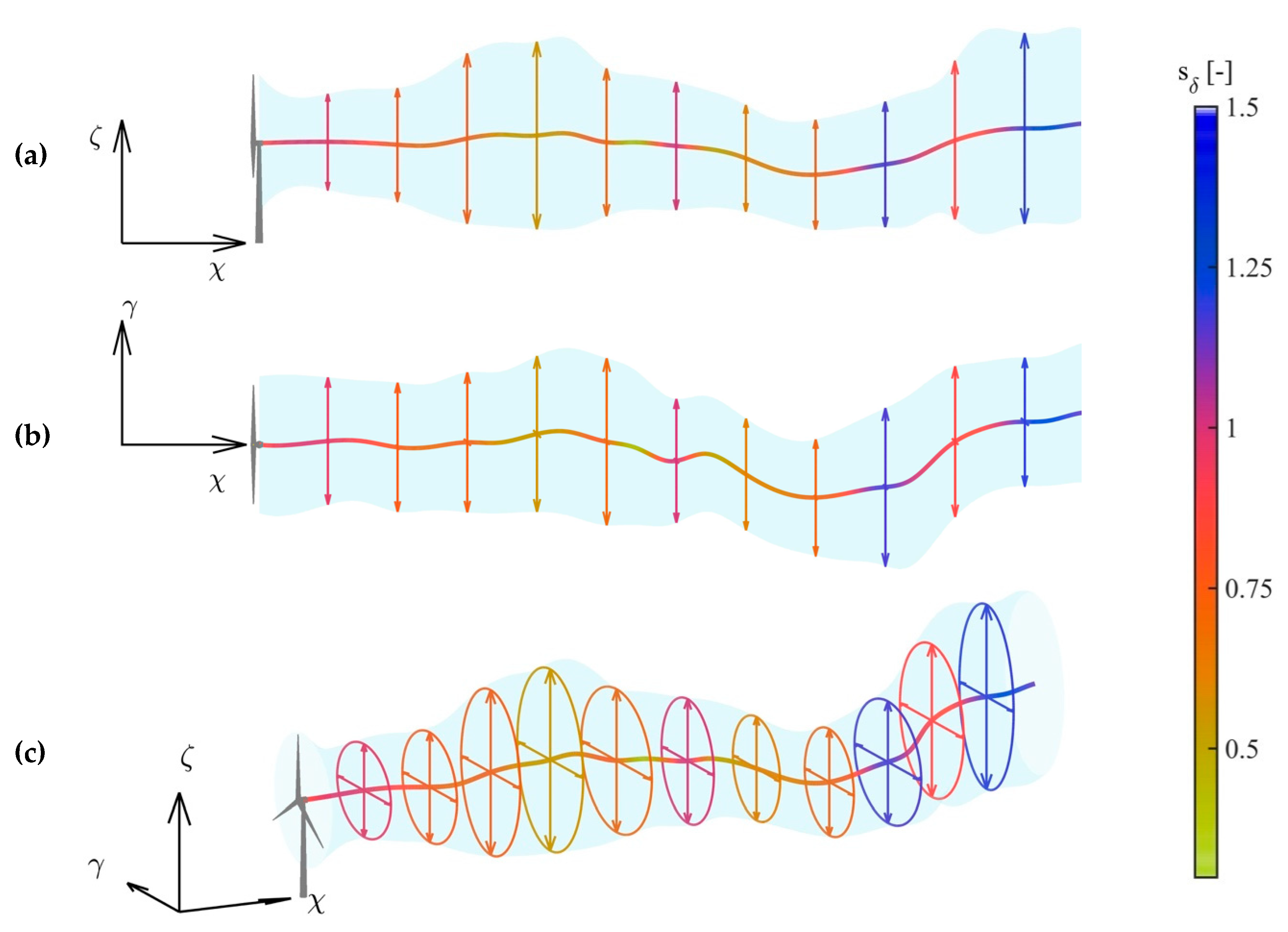
  • If we consider a cross-section of a wake wind field in the γ ζ plane at a certain downstream distance χ , the resulting flow behavior of the longitudinal wind speed component u of the wake can be described as a superposition of the free flow with a planar (two-dimensional (2D)) longitudinal wind speed deficit, which shows specific transversal dynamics.
  • We define these dynamics as temporal changes in the horizontal and vertical positions, the horizontal and vertical velocity deficit shapes, and the velocity deficit intensity, which represents the ratio of the tracked wake velocity at the wake center to the instantaneous ambient wind speed profile. These dynamics will be described below as the wake center position, wake width, and wake velocity intensity in 2D and later 3D.
  • The wake velocity deficit causes a scaling of the ambient turbulence intensity, which depends on the 2D deficit shape at the downstream position χ . Other than the ambient turbulence intensity scaling, no additional turbulence is added as the meandering of the deficit shape induces turbulence.
  • If we apply these considerations continuously in the downstream direction, we can consider the wake region a continuous symmetrical wake volume centered around a spline in space that alters depending on the previously described dynamics.
  • The wake velocity deficit intensity is variable in time and space.
To gain a better understanding, we visualized the reconstruction assumptions in Figure 2 for one point in time. The wake is shown as a continuous tube that tapers and widens along the wake center line in the horizontal and vertical directions, respectively. The template for modifying and scaling this tube was a volumetric velocity deficit, which we created from the LiDAR measurements. Different colors within the wake region in Figure 2 represent the variable instantaneous intensities of planar deficits at the corresponding downstream positions.
Below, we present the processing steps applied to obtain the wind speed deficit, the shape dynamics, the intensity dynamics, and the position dynamics from LiDAR data for use in wind-field reconstruction.

3.1. LiDAR Data Pre-Processing

Because this study represents a further development of Beck and Kühn [22], we used the same data handling in the sense of pre-processing, up-sampling, and synchronization, as well as the same numerical dataset. Therefore, we directly quote the formal description of the dataset and use the essential parts. The complete data processing method can be read in Reference [22].
To deduce the instantaneous longitudinal wind speed component ( u 0 ) from LiDAR radial velocity data ( υ ^ L O S ), we assumed that within the 10-min interval, the average lateral velocity component ( v ¯ 0 ) and average vertical velocity component ( w ¯ 0 ) were zero. Recognizing that this assumption did not apply near the rotor ( χ D 1 3 ), we calculated u as follows:
u 0 = υ ^ L O S cos ( ϕ ) cos ( θ ) ,
where ϕ is the difference between the horizontal wind direction ( Φ ) and azimuth angle ( ϕ ), and θ is that between the vertical wind direction ( Θ ) and elevation angle ( θ ).
The projection of LOS velocities was made scanwise and, thus, individual scans were interpolated to a Cartesian ( χ - γ , γ - ζ ) coordinate grid using the natural neighbor interpolation [34].
Like Beck and Kühn [22], the standard deviation was calculated using the previously calculated LOS velocity projection to the longitudinal wind speed component ( u 0 ). This pragmatic approach had the consequence that not the longitudinal wind speed component’s original turbulence intensity ( I 0 ), but only the statistics of the projected LOS velocities ( υ ^ L O S ), could be constructed.

3.2. Temporal Correction and Lidar Data Synchronization

Because of the scanning measurements of PPI and RHI scans, it was not possible to capture the entire measurement area at one point in time. This restriction resulted in a representation of the wind field over a time interval of the scan, as shown Table 1. Therefore, we did not directly use the measured and projected LiDAR data for further processing. Slower scan speeds resulted in more significant temporal shifts within a scan (Figure 3). Furthermore, the temporal resolution of the tracked wake dynamics (Section 3.3) became insufficient.
We used Beck and Kühn’s [22] temporal up-sampling method to interpolate the synthetic LiDAR data to the LES reference time step. This method uses a simplified 2D Navier–Stokes equation that contains only the advection term implemented using an affine semi-Lagrange interpolation approach. A sinusoidally weighted combination of forward- and backward-oriented space–time conversions resulted in the closure of each LES grid point of the flow field between two consecutive scans.
Figure 3 shows how the wind-field propagation minimizes the time shift within one scan (dark blue), where the horizontal axis represents time and the vertical axis indicates the LiDAR measurement’s current scan angle. The scanning from ϕ 1 to ϕ 2 is drawn over the scanning period T ϕ in dark blue. For the return run during the reset time ( t r ), the scanner head must start a new trajectory without measuring. The return run is illustrated in green, and the propagated scans are shown in light blue. Applying the wind-field propagation [22] allowed an increase in the number of intermediate steps (light blue) between two consecutive scans by an arbitrary number. To correct the time shift and represent the flow at one point in time ( t ) and not over the entire time interval ( T ϕ + t r ), we interpolated along the red line using the natural neighbor interpolation [34]. Here, it became apparent that a shorter propagation time step yielded more accurate temporal mapping of a scan.
We up-sampled the LiDAR data based on the scanning velocity and improved the amount of data by factors of 2.4–40, to achieve a resolution of 1 Hz. The wind-field propagation result was a 10-min dataset of 600 planar PPI and RHI scans, which were synchronized mutually and with the LES reference. These data constituted the initial basis for the temporally resolved wake dynamic determination.

3.3. Determination of Wake Deficit Dynamics

Two sets of information were needed for wind-field reconstruction: the wind speed deficit and its dynamics. The significant issue here was the characterization of the wake dynamics, namely, the wake position, the wake width, and the velocity deficit intensity over time, as these data were also used for calculating the velocity deficit shape in the MFoR [8,9,35] in Section 3.4 and the standard deviation of longitudinal wind speed component u in the MFoR in Section 3.5. This led to the reconstruction quality having a direct dependency on the tracked values, with their precision and their expressiveness concerning real flow situations. Like other studies [19,20,35], we applied a robust Gaussian curve fitting based on Brent’s [36] optimization approach on the temporally aligned and synchronized wind speed dataset. Therefore, we firstly normalized the dataset with the 10-min averaged vertical wind speed profile ( u ¯ 0 ( ζ ) ) to obtain u ( χ , γ , ζ , t ) as the normalized longitudinal wind speed.
u ( χ , γ , ζ , t ) = u 0 ( χ , γ , ζ , t ) u ¯ 0 ( ζ ) .
In our study, we obtained this wind speed profile by averaging the LES wind field far upstream of the simulated turbine. In actual LiDAR measurements, one can use downstream measurements well outside of the wake-affected region.
We applied the following functions as the wake-tracking approach:
u f i t , P P I ( χ , r γ , t ) =   β γ ( χ , t )     α γ ( χ , t ) σ γ ( χ , t )   2 π e 1 2 ( r γ μ γ ( χ , t ) σ γ ( χ , t ) ) 2 ,
for horizontal scans and
u f i t , R H I ( χ , r ζ , t ) =   β ζ ( χ , t )     α ζ ( χ , t ) σ ζ ( χ , t )   2 π e 1 2 ( r ζ μ ζ ( χ , t ) σ ζ ( χ , t ) ) 2 ,
for vertical scans, with r γ and r ζ as coordinates in the respective transversal in-plane directions relative to the downstream direction χ . For a better understanding of the relationship between the fitting variables and wake velocity, we present a general application of Equations (6) and (7) for the RHI and PPI scans in Figure 4, respectively. μ γ and μ ζ depict the wake center position (light blue), σ γ and σ ζ indicate the characteristic wake width (turquoise), α γ and α ζ denote the deficit intensity (yellow), and β γ and β ζ indicate the ambient longitudinal wind speeds (green). In contrast to Aitken et al. [19] and Bromm et al. [20], who employed a double Gaussian function for the near-wake region ( χ D 1 < 2) to represent the characteristic deficit form, we used a threshold that does not consider data below a normalized velocity of 0.55. As a result, tracking was robust and numerically faster to calculate, compared to double Gaussian fitting. By omitting velocities up to the threshold, the algorithm mainly fit the high shear flanks of the wake deficit. The subsequent application of Equations (6) and (7) to the propagated horizontal and vertical data from Section 3.2 resulted in a temporal dependency of the tracked values.

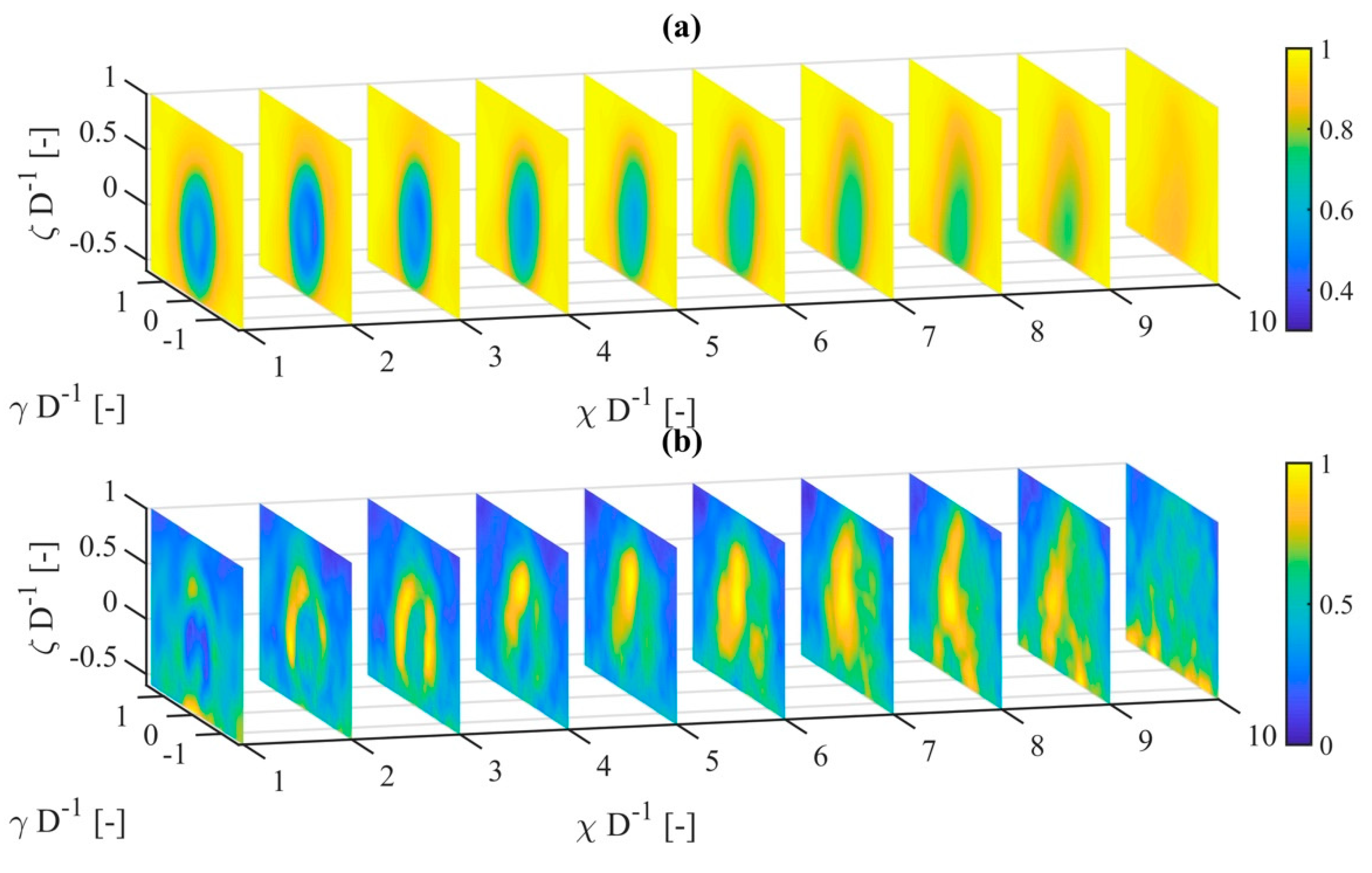
3.4. Calculation of the Volumetric Wind Speed Deficit

Section 3.3 showed how wake tracking was used to determine wake dynamics from temporally up-sampled and synchronized RHI and PPI scans. In this section, we describe how the reconstructed wake deficit is calculated.
To correctly depict the averaged wake deficit at downstream distance χ in the reconstructed wind field, a change in perspective was required to understand why the measured velocities from the RHI and PPI scans could not be directly used within the reconstructed wind field. The averaged wake deficit in the fixed frame of reference ( δ F F o R ¯ ) was the convolution of temporally resolved deficits ( δ M F o R ). Within the DWM model, these temporally resolved deficits are considered constant and observed in the MFoR that moves with the wake center. In contrast, we regarded temporally resolved deficits ( δ M F o R ) as variable, with an average deficit ( δ M F o R ¯ ) that resulted in an averaged wake deficit in the FFoR ( δ F F o R ¯ ) when convoluted according to the wake dynamics. We obtained these wake dynamics in Section 3.3. The synchronized RHI and PPI scans constituted the dataset for the average deficit in the MFoR ( δ M F o R ¯ ), which in turn was a convolution of the variable temporally resolved deficits in the MFoR ( δ M F o R ).
In the test case presented here, flow information was available only on the cross-shaped measurement planes. Because the LiDAR-measuring planes were fixed in the FFoR, the wake moved dynamically through them. Therefore, the variable temporally resolved deficits in the MFoR ( δ M F o R ) were measured at different radial positions in the FFoR, depending on the wake center position. If we look at a γ - ζ plane at downstream distance χ , only two lines of information are available. To obtain a planar deficit in the γ - ζ plane, we assumed a conditional point symmetry for the wake deficit by rotating the vertical and horizontal LiDAR scans from −90° to 90° (Figure 5b). If we extended the consideration of the wake deficit in a γ - ζ plane with a spatial dimension in downstream direction χ , the lines of information became planes of information and the planar deficit became a volumetric deficit (VD).
We used propagated RHI and PPI wind speed data ( u ), which were combined in a Cartesian ( χ ,   γ ,   ζ ) coordinate system. To obtain volumetric information from planar horizontal data u PPI ( χ , γ , h HH , t ) and planar vertical data u RHI ( χ , 0 , ζ , t ) , we assumed a conditional rotational symmetry to create a closed volumetric deficit over downstream distance χ . Thus, we firstly defined the volumetric wind speed average in the MFoR ( u VD MFoR ¯ ) . The change from the turbine-based coordinate system to the MFoR can be expressed as
γ ( χ , γ , t ) = γ μ γ ( χ , t ) ,
and
ζ ( χ , ζ , t ) = ζ μ ζ ( χ , t ) .
To improve the formula’s readability, we did not refer further to the dependence of initial variables ( γ and ζ ), but rather a reference system based on the new variables ( γ and ζ ) as a new coordinate system.
The definition of the volumetric wind speed average in the MFoR ( u VD MFoR ¯ ) in Equation (10) aims to describe the average wake wind from the rotor without meandering effects.
u VD MFoR ( χ , γ , ζ ) ¯   =   1 | T | t     T u r o t ( χ , γ , ζ , t ) .
Although this is clearly visible on the left side, the right side implies the reference frame change by subtracting the wake center ( μ γ and μ ζ ) from the γ and ζ coordinates within the wind field (Equations (8) and (9)). From the conditional rotational symmetry (±90°), we defined the wind speed calculation for a corresponding point within the resulting four quadrants.
u r o t ( χ , γ , ζ , t ) = { ( 1 λ ( χ , γ , ζ , t ) ) · u PPI ( χ , sign ( γ ) · τ , h HH , t ) + λ ( χ , γ , ζ , t ) · u RHI ( χ , 0 , sign ( ζ ) · τ , t ) |   γ 0 , ζ 0 u RHI ( χ , 0 , ζ , t ) |   γ = 0 , ζ 0 u PPI ( χ , γ , 0 , t ) |   γ 0 , ζ = 0 1 2 ( u PPI ( χ , 0 , h HH , t ) + u RHI ( χ , 0 , 0 , t ) ) |   γ = 0 , ζ = 0 ,
and
λ ( χ , γ , ζ , t ) = | 2 tan 1 ( ζ ( χ , t ) γ ( χ , t ) ) π | ,
as the rotational weighting function and
τ = γ 2 + ζ 2 , 2
as the radius within the MFoR. Here, T represents a set with t     T containing all wind speed information at a discrete time point t within the studied 10-min time interval. The use of dashes in Equation (10) indicates the cardinality of set T . Equation (10) implies that the wake center’s position was displaced in the γ -direction and ζ -direction with respect to the hub height center line before the corresponding velocities were rotated and weighted (Equation (11)) to calculate the mean value ( u V D M F R ¯ ) . This was the turbine-emitted wake average without any horizontal and vertical meandering effect.
Figure 5 visualizes the conditional rotational symmetry introduced in Equation (11). Figure 5a shows how the velocity of any point in the MFoR—not only on the measuring axes—was calculated by the weighting factors λ and 1     λ from the RHI and PPI data, respectively, depending on the point’s position. In Figure 5b, we visualize the rotational weighting factor ( λ and 1 λ ) as a function of the rotation angle depending on the position in the MFoR.

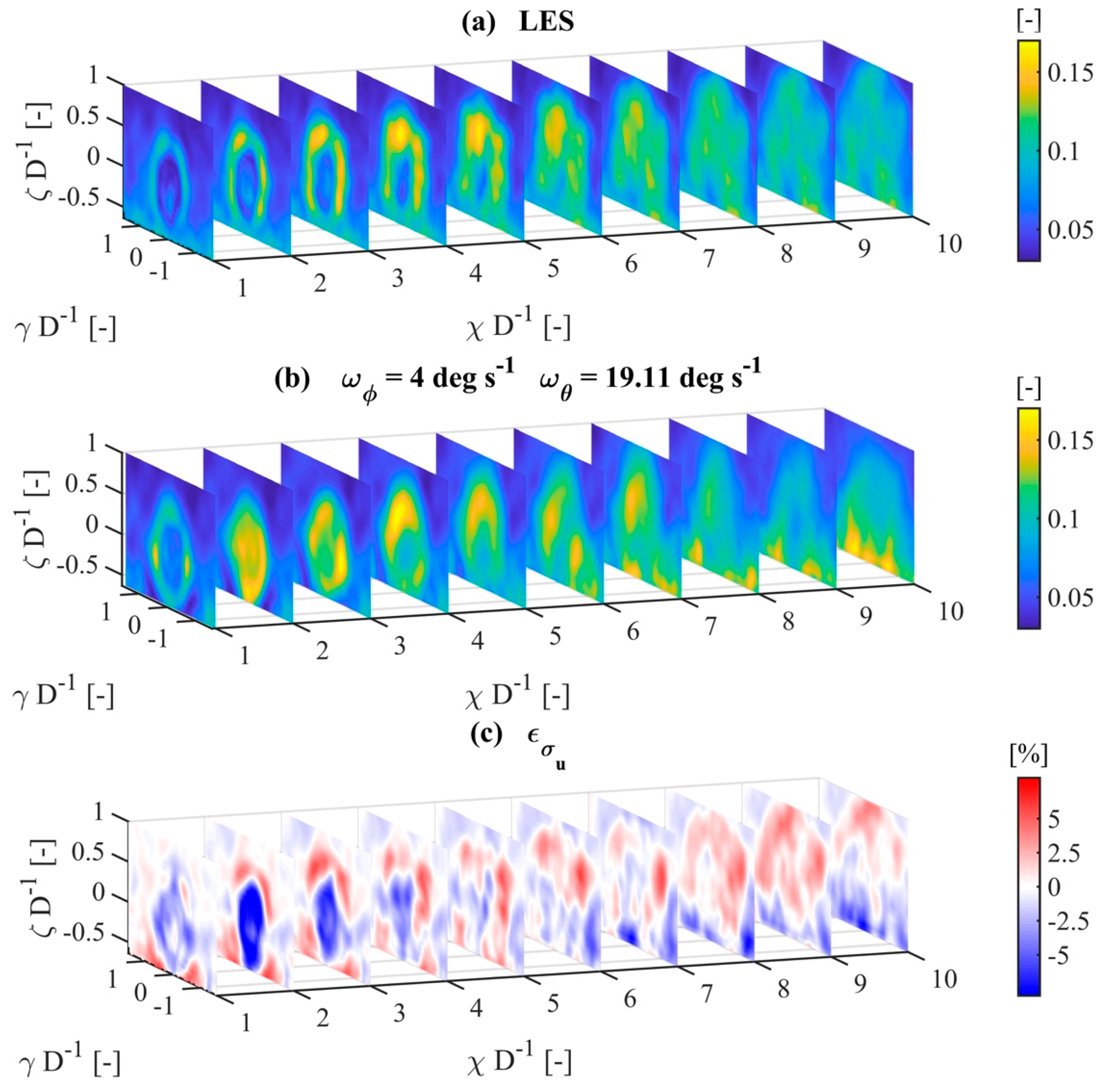
3.5. Calculation of the Volumetric Turbulence Intensity Scaling

Analogous to generating the three-dimensional wake velocity field ( u VD MFoR ¯ ) , we calculated the standard deviation of the velocities ( σ VD MFoR ) in the MFoR as
σ VD MFoR ( χ , γ , ζ ) = 1 | T |   t     T ( u ( χ , γ , ζ , t ) u VD MFoR ( χ , γ , ζ ) ¯ ) 2 ,
where σ VD MFoR indicates the variability within the meander-free wake velocity field u VD MFoR ¯ , and is used to scale ambient turbulence to represent the turbulence induced by the wake itself without meandering-induced turbulence. To generate the turbulence intensity scaling factor ( s I 0 MFoR ) from σ VD MFoR , we firstly normalized it with u VD MFoR ¯ to obtain the turbulence intensity within the MFoR, and then divided the result by the atmospheric turbulence intensity profile I 0 ( ζ ) .
I VD MFoR ( χ , γ , ζ ) = σ VD MFoR ( χ , γ , ζ ) u VD MFoR ¯ ( χ , γ , ζ ) ,
s I 0 MFoR ( χ , γ , ζ ) = I VD MFoR ( χ , γ , ζ ) I 0 ( ζ ) .

3.6. Four-Dimensional Wake Wind-Field Reconstruction

In this section, we explain how the wake dynamics determined in Section 3.3, the volumetric wake field ( u VD MFoR ¯ ) determined in Section 3.4, and the turbulence scaling factor ( s I 0 MFoR ) determined in Section 3.5 were combined to reconstruct a 3D1C wake wind field.
The reconstruction’s starting point was a 3D1C ambient flow wind field created by a wind field generator with freely selectable dimensions matching the atmospheric parameters from Section 2. We decomposed the generated wind field’s longitudinal velocity component ( u a ) into constant ( u a ¯ ) and fluctuating ( u t ) parts.
u a ( χ , γ , ζ , t ) = u a ( χ , γ , ζ ) ¯ + u t ( χ , γ , ζ , t ) .
Here, we defined the mean wake deficit in the MFoR as the difference between the wake velocity field and the normalized ambient flow.
δ VD MFoR ( χ , γ , ζ ) ¯ =   1 u VD MFoR ( χ , γ , ζ ) ¯ .
The average volumetric deficit in the MFoR ( δ VD MFoR ¯ ) served as a template in the form of a flexible tube that was displaced and scaled by the dynamics ( μ γ ( χ , t ) , μ ζ ( χ , t ) , σ γ ( χ , t ) , σ ζ ( χ , t ) , α γ ( χ , t ) , α ζ ( χ , t ) , β γ ( χ , t ) , and β ζ ( χ , t )).
To recreate the original dynamic wake behavior as a volumetric deficit, we defined three time- and space-dependent scaling factors as follows:
s γ ( χ , t ) = σ γ ( χ , t ) σ γ u VD MFoR ¯ ( χ ) ,
which represents the horizontal spatial deficit shape scaling factor;
s ζ ( χ , t ) = σ ζ ( χ , t ) σ ζ u VD MFoR ¯ ( χ ) ,
which represents the vertical spatial deficit shape scaling factor; and
s δ ( χ , t ) = 1 2 1 2 π ( α γ ( χ , t ) σ γ ( χ , t ) + α ζ ( χ , t ) σ ζ ( χ , t ) ) + β γ ( χ , t ) + β ζ ( χ , t ) 1 2 π ( α γ u VD MFoR ¯ ( χ ) σ γ u VD MFoR ¯ ( χ ) + α ζ u VD MFoR ¯ ( χ ) σ ζ u VD MFoR ¯ ( χ ) ) + β γ ( χ ) + β ζ ( χ ) ,
which represents the velocity deficit intensity scaling factor. Here, μ γ u VD MFoR ¯ ( χ ) , μ ζ u VD MFoR ¯ ( χ ) , σ γ u VD MFoR ¯ ( χ ) , σ ζ u VD MFoR ¯ ( χ ) , α γ u VD MFoR ¯ ( χ ) , α ζ u VD MFoR ¯ ( χ ) , β γ u VD MFoR ¯ ( χ ) , and β ζ u VD MFoR ¯ ( χ ) were determined by applying Equations (6) and (7) to the vertical and horizontal slices through the hub height center line of the 3D u V D M F o R ¯ . Thus, it became apparent that u V D M F o R was only scaled by the three previously defined factors because of its descriptive properties.
This led to the resulting formula for generating the time-dependent 3D1C velocity deficit ( δ V D ). Here, we applied retransformations from the MFoR on the right sides of Equations (22) and (23) to the FFoR on the left side of these equations, by adding the wake center position ( μ γ and μ ζ ).
δ V D ( χ , γ , ζ , t ) = δ VD MFoR ( χ , γ · s γ ( χ , t ) + μ γ ( χ , t ) , ζ · s ζ ( χ , t ) + μ ζ ( χ , t ) ) ¯ · s δ ( χ , t ) .
Analogously, the resulting formula for the four-dimensional (3D1C) turbulence scaling could be expressed as
s I 0 ( χ , γ , ζ , t ) = s I 0 MFoR ( χ , γ · s γ ( χ , t ) + μ γ ( χ , t ) , ζ · s ζ ( χ , t ) + μ ζ ( χ , t ) ) · s δ ( χ , t ) .
To describe the reconstructed wake field ( u RC ), we assumed a superposition approach similar to Equation (17). The constant part of the ambient wind field ( u a ¯ ) was overlaid with the dynamic wake deficit ( δ V D ), and the fluctuating part of the ambient wind field ( u t ) was multiplied by the dynamic turbulent intensity factor ( s I 0 ). This defined the reconstructed wake field ( u RC ) .
u R C ( χ , γ , ζ , t ) = ( u a ( χ , γ , ζ ) ¯ δ V D ( χ , γ , ζ , t ) ) + ( u t ( χ , γ , ζ , t ) · s I 0 ( χ , γ , ζ , t ) ) .

4. Results

In this section, we present results of the reconstruction method introduced in Section 3 to work with the synthetic LiDAR data described in Section 2. To the extent possible, we varied the angular velocities ω ϕ and ω θ to determine their influences on reconstruction quality, thereby finding an optimal parameter set for the test case.

4.1. Determination of Wake Dynamics

We determined the wake dynamics by applying the Gaussian wake tracking method from Section 3.3 on the propagated LiDAR and LES wind speed data. The determined wake dynamics appeared to be the most influencing factors for reconstruction as the corresponding results were also used to calculate the deficit shape. To evaluate the wake tracking quality from the propagated LiDAR scan data, we referred to the LES wind field. Thus, we applied Equations (6) and (7) to the LES data and estimated the wake center position dynamics, which we used as a reference in our analysis.
Figure 6 shows a visualization of the tracked wake center depending on time and the dimensionless downstream position χ D 1 . Figure 6i shows a consistent mapping of the wake path and depicts lateral meandering effects over the downstream direction χ and time t . Unphysical jumps or fractures, which indicate that the chosen method cannot be representative or that the chosen spatial and temporal resolutions are insufficient, were not visible. Individual flow structures tracked in the downstream direction over time, which we refer to as meander events, are shown as curved stripes in Figure 6. As expected, meander events were characterized by increasing lateral deflections and advection speeds with increased downstream distance.
Noisy behavior can be recognized for all angular velocities up to a distance of χ D 1 3 for the wake center data μ γ D 1 in Figure 6a–h. This noise occurred due to the insufficient data availability in the γ -direction outside of the scanned area, which was determined by the scanning opening angle Δ ϕ .
Because of the influences of the wind-field propagation boundary condition, the wind speed was reduced at a downstream distance of χ D 1 10 . This influence was attributed to the space–time conversion boundary conditions and could also be seen in the wake dynamics determination. Compared to the LES, a significant periodic deviation of the tracked wake center was visible at the rear edge of the measuring area around χ D 1 10 , which distracted the Gaussian fitting function from the real wake deficit. The frequency and size of this distraction depended on the number of propagation steps and decreased as the number of steps decreased. Gaps in Figure 6 show that the Gaussian fitting could not always determine a clear parameterization. The corresponding illustration of the RHI scan-tracked wake center positions can be found in Appendix A.
Although the influence of the wind-field propagation on the wake dynamic tracking could not be bypassed here, the fitting algorithm’s performance in situations with insufficient data, i.e., for χ D 1 3 , could be significantly improved by artificially adding data from the corresponding scan. For this purpose, unavailable data in Figure 7a, outside of the red circular arc-shaped area visible in Figure 7b, were added within the χ -direction averaged wind speed values for the corresponding γ -positions from the corresponding scan. For averaging, we considered wind speed 0.25 D from the first available data in the χ -direction for the corresponding γ -positions. Figure 7b shows how the artificial data extension (ADE) added spatially averaged data to complement unavailable data due to the opening angle of the measurement.
Figure 8 and Figure 9 demonstrate the effects of ADE (Figure 8b,d and Figure 9b,d) on horizontal tracking results compared to the original data (Figure 8a,c and Figure 9a,c) and provide an overview of the tracked value statistics.
Figure 8a,b show the mean value (solid lines) μ γ ¯ of the tracked horizontal wake center μ γ and its standard deviation (dashed lines) σ μ γ for different angular speeds, and Figure 8c,d display the averaged tracked horizontal wake width (solid lines) σ γ ¯ of σ γ and its standard deviation (dashed lines) σ σ γ . An almost linear lateral displacement of the wake center of approximately 0.17 D could be seen over a downstream distance of 10 D, which corresponded to an approximately 1° deflection angle. Here, the effects of insufficient data and the influence of boundary conditions could be seen in the strong deviations. By applying ADE, we inferred from Figure 8b that the wake center position of the propagated wind speed data could be determined more precisely, not only up to χ D 1 3 but over the entire flow field. This was evident for all angular velocities and could be seen in the mean value μ γ ¯ and in the wake center’s standard deviation σ μ γ . The wake dynamics determination improvements are particularly noticeable in the tracked horizontal wake width in Figure 8d. Although the mean wake width σ γ ¯ was accurately represented for downstream distances χ D 1 > 3 , the most significant improvement was noted in the wake width’s standard deviation (dashed lines) σ σ γ , which was better tracked over all downstream positions.
Videos S1 and S2 (Supplementary Materials) for the horizontal and vertical data, respectively, show not only propagated wind speed data but also the wake tracking results. The black line indicates the wake center’s position based on the propagated data, whereas the white line was based on ADE results. It is clearly visible that the accuracy and variability of the position tracking could be improved with the above presented approach up to χ D 1 3 .
We identified, mainly through visual comparison, two factors in tracking vertical wake movements that we found to be more susceptible to interference than in horizontal tracking. Firstly, because vertical velocity data were measured on the center line, only this wake deficit was displayed on the vertical plane for the horizontal wake profile. It was, thus, not ensured that the tracking algorithm would identify the wake deficit in the case of pronounced horizontal meandering. The effects of limited representativeness of the intersection of the measurement planes and the current wake volume were more evident for vertical measurements than horizontal measurements as the horizontal wake displacement was characterized by greater amplitudes than vertical wake displacement. This different behavior shows the necessity of wake tracking methods that do not quantify instantaneous wake profile integrally, but rather use a separate method optimized for vertical wake measurements. The amplitude difference cannot be seen in the statistics in Figure 8 and Figure 9, as they already include effects of limited representativeness of the measured intersection; however, they can be observed in Videos S1 and S2 (Supplementary Materials).
The second influencing factor was the LiDAR simulator’s operating principle. When laser pulses hit the ground, a hard target is simulated, which results in corrupted velocity data. These data gaps result in a reduced amount of data that affect the fitting quality.
As in Figure 8, we illustrate vertical wake-tracking statistics in Figure 9a,b, which show the mean value (solid lines) μ ζ ¯ and its standard deviation (dashed lines) σ μ ζ . We can see that the wake gradually sank to −0.2 D over the entire downstream distance. This can be clearly observed at a distance of χ D 1 > 3 , after which the corresponding standard deviation increased almost linearly. At a distance of χ D 1 > 8 , the accuracy of μ ζ ¯ of ω θ 19.11 ° / s decreased due to ADE. A possible explanation for this was the reduced data availability near the ground, which was amplified by the lesser number of angular measurements (Table 1).
In Figure 9c,d, we present the average vertical wake width σ γ ζ ¯ and the standard deviation σ σ ζ . Here, the difficulties of tracking the vertical wake profile become apparent. If we regard the original (Figure 9c) and ADE (Figure 9d) vertical wake width results, we can find that σ γ ζ ¯ does not reflect a smooth trend, as expected from the horizontal tracking. The ADE data showed a better representation of the wake expansion at χ D 1 1 , which could also be found in the LES reference data. Furthermore, the standard deviation of the wake width σ σ ζ could be improved, especially in the near-wake region of χ D 1 < 3 .
Within the subsequent reconstruction process steps, we used ADE to represent the wake dynamics.

4.2. Four-Dimensional Wake Wind-Field Reconstruction

In this section, we present the 3D1C wake wind-field reconstruction results. Because the comparison of time-dependent wind fields can be quantified using different approaches, we firstly discuss the reconstruction quality’s dependence on horizontal and vertical angular velocities as the main influencing factors for spatial and temporal discretization of the wake region. Then, we show the most accurate reconstructed wake wind field. To this end, we differentiated the reconstruction quality into steady and dynamic approaches.

4.2.1. Steady Error Quantification

Various methods can be used to quantify the comparability of time series in time-series analysis. One assumption is the consideration of signals as discrete stochastic processes. Central moments can be compared using a finite amount of sample data. Here, we considered the first moment in the form of mean value differences, expressed as
ε u ¯ = u R C u L E S ,
with index RC representing the reconstructed wake wind field and index LES representing the LES reference wind field. Similarly, we analyzed the second moment in the form of standard deviation errors expressed as
ε σ u = σ R C σ L E S .
Below, we limit the discussion of the results to an averaged evaluation for 4 χ D 1   9 to exclude the propagation errors at the flow field outlet and near-rotor area because of the assumed homogeneity. This choice gives a stronger focus on commonly used turbine spacing.
Figure 10a shows the average error of the 3D1C reconstructed wake wind field of corresponding angular velocity combinations with respect to the original LES wake wind field. A clear minimum of ε u ¯ = 2.3   % can be seen for the combination of ω ϕ   =   12 ° / s and ω θ   =   19.11 ° / s . From this minimum, an exponential increase in error can be detected on both axes, where a greater error increase for ω θ than ω ϕ indicates a greater dependency on vertical scanning than horizontal scanning. The standard deviation error distribution in Figure 10b indicates that, for ω ϕ   =   12 ° / s and ω θ   =   8 ° / s , it was possible to reconstruct the standard deviation with ε σ u = 0.16   % . Furthermore, a clear trend can be observed in the error. Combinations showing a small error formed an exponential behavior for angular velocities of up to ω ϕ     12 ° / s , after which they mainly depended on ω θ . This means that reconstructing a wake fluctuation with a low horizontal temporal resolution could be compensated for by using a high vertical temporal resolution. From this behavior, we deduced a greater dependence of the reconstruction on vertical measurements than horizontal measurements. Figure 10a,b show that the reconstruction could be parameterized to minimize either the average wind speed error or standard deviation error. Because of the wake reconstruction method’s complexity, we could not provide a detailed justification in this respect and could only evaluate the results as a whole. However, because a major part of the method is based on wake dynamics, we could assume that a wake tracking method that is more representative of the real wake dynamics also provides more precise reconstruction results.
Because we assumed that both the average and the standard deviation should be accurately reflected in the reconstruction, Figure 10c presents the combined error behavior of
ε CMB = ε u ¯ 2 + ε σ u 2 ,
to determine a trade-off representing a resulting minimum at ω ϕ   =   4 ° / s and ω θ   =   19.11 ° / s .
We used this angular velocity combination as a compromise to show differences between the reconstructed wind field and original LES wind field. Therefore, we present γ ζ -planes for different downstream distances in Figure 11 and Figure 12, to depict the distribution of the wind speed average, the standard deviation, and the related errors ε u ¯ and ε σ u .
The reconstructed wake wind field in Figure 11b can represent the expansion and relaxation of the velocity deficit in the downstream direction corresponding to the LES reference in Figure 11a. The wind speed error in Figure 11c demonstrates an underestimation of the deficit that could be observed for all distances within a structure and was more imposed in the vertical direction. We assumed that this was based on the weaker representation of wake dynamics by the wake tracking method for vertical measurements than horizontal measurements. The importance of this on the overall reconstruction could be seen here.
Because of the conditional rotational symmetry and the limited data availability due to the horizontal and vertical scan opening angles, increased errors were to be expected in the mean wind speed and standard deviation up to χ D 1 3 . We first noted this in the velocity deficit of the turbine tower, which could be detected in the first downstream slice at χ D 1 = 1 in Figure 11a and Figure 12c, but could not be mapped in the reconstruction in Figure 11b. Furthermore, it was found in the reconstructed deficit profile in a radial direction up to χ D 1 2 . Additionally, it was evident that the distribution of the standard deviation up to χ D 1 3 was strongly underestimated in the wake region (Figure 12c). Moreover, the standard deviation in Figure 12a,b showed that the areas of increased fluctuation were more strongly affected by errors than the initial horizontal and vertical plane positions because of the rotational symmetry. Figure 12c shows this effect in the downstream planes 2     χ D 1 6 . We surmised that this effect was due to spherical-to-Gaussian sub-grid interpolations.
A further assumption-induced error could be seen up to χ D 1 6 due to the absence of a wake-soil model. The apparent velocity increase near the ground could not be reproduced in the reconstruction. This error could also be seen in the standard deviation differences in Figure 12c.
To give an overall impression of the reconstructed wind field behavior, we present vertical slices at different downstream distances in Video S3 (Supplementary Materials), which shows the wind speed compared to the LES. The reconstructed wind field in Video S3 was calculated using the parameterization of ω ϕ   =   4 ° / s and ω θ   =   19.11 ° / s .

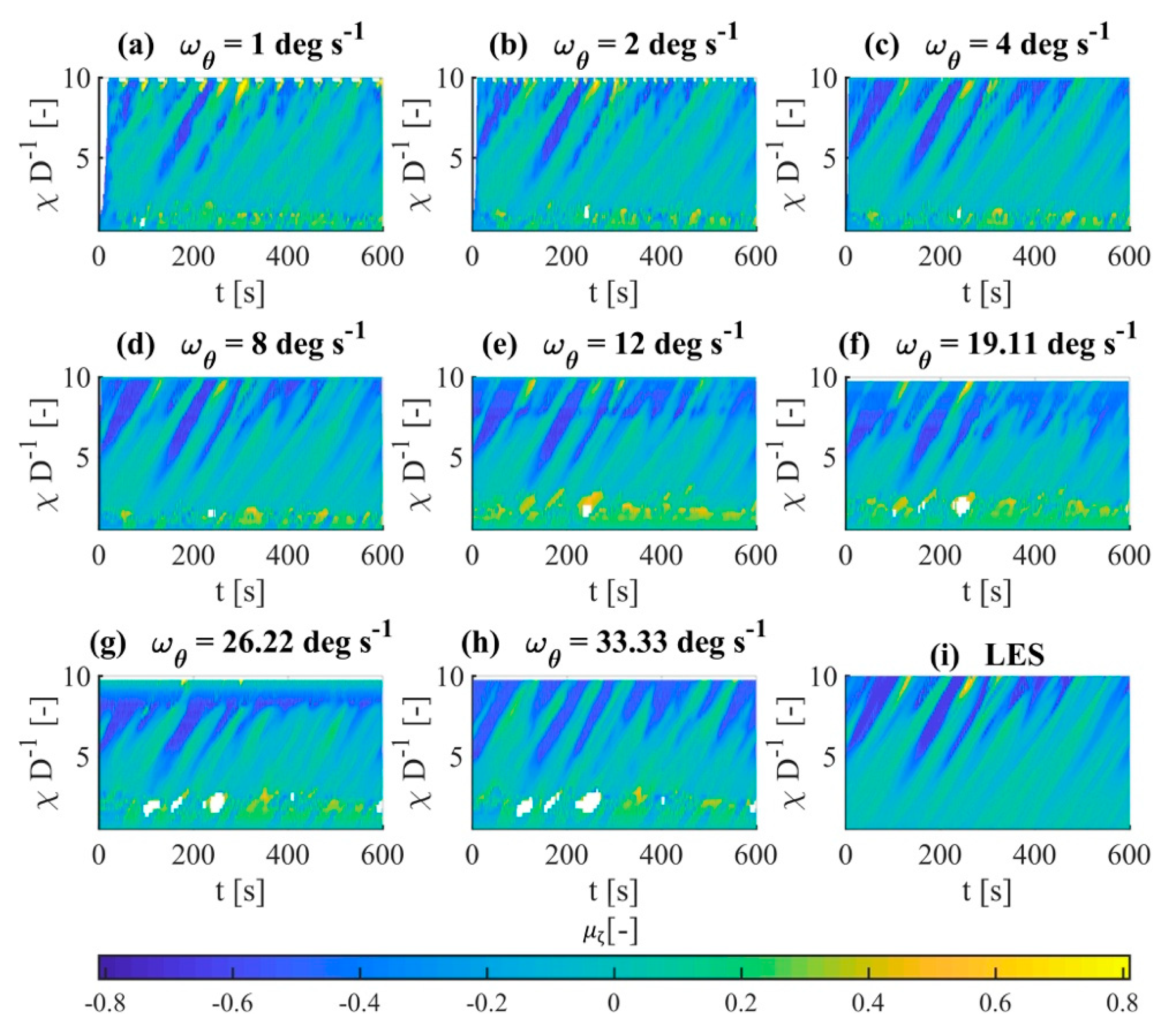
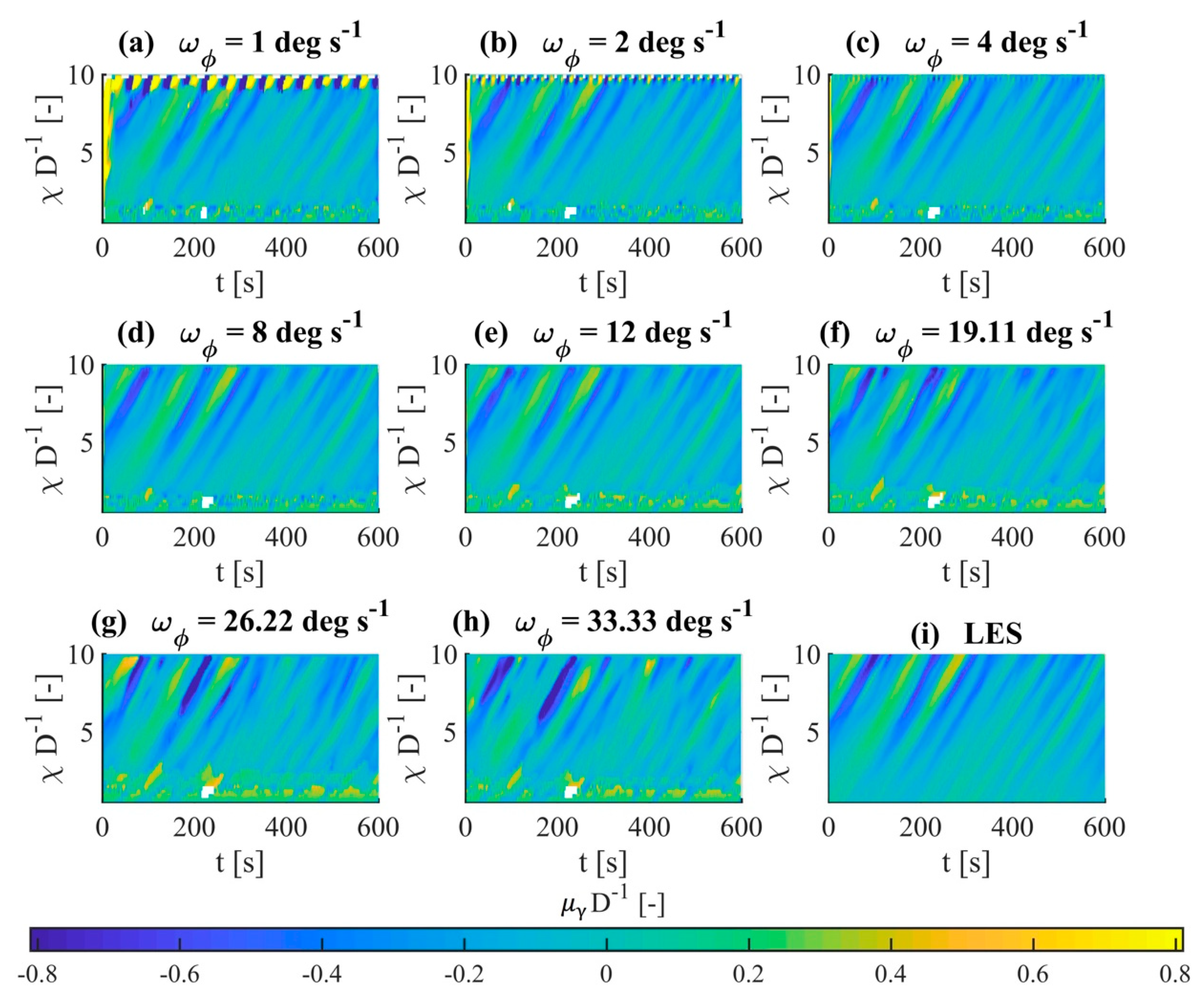
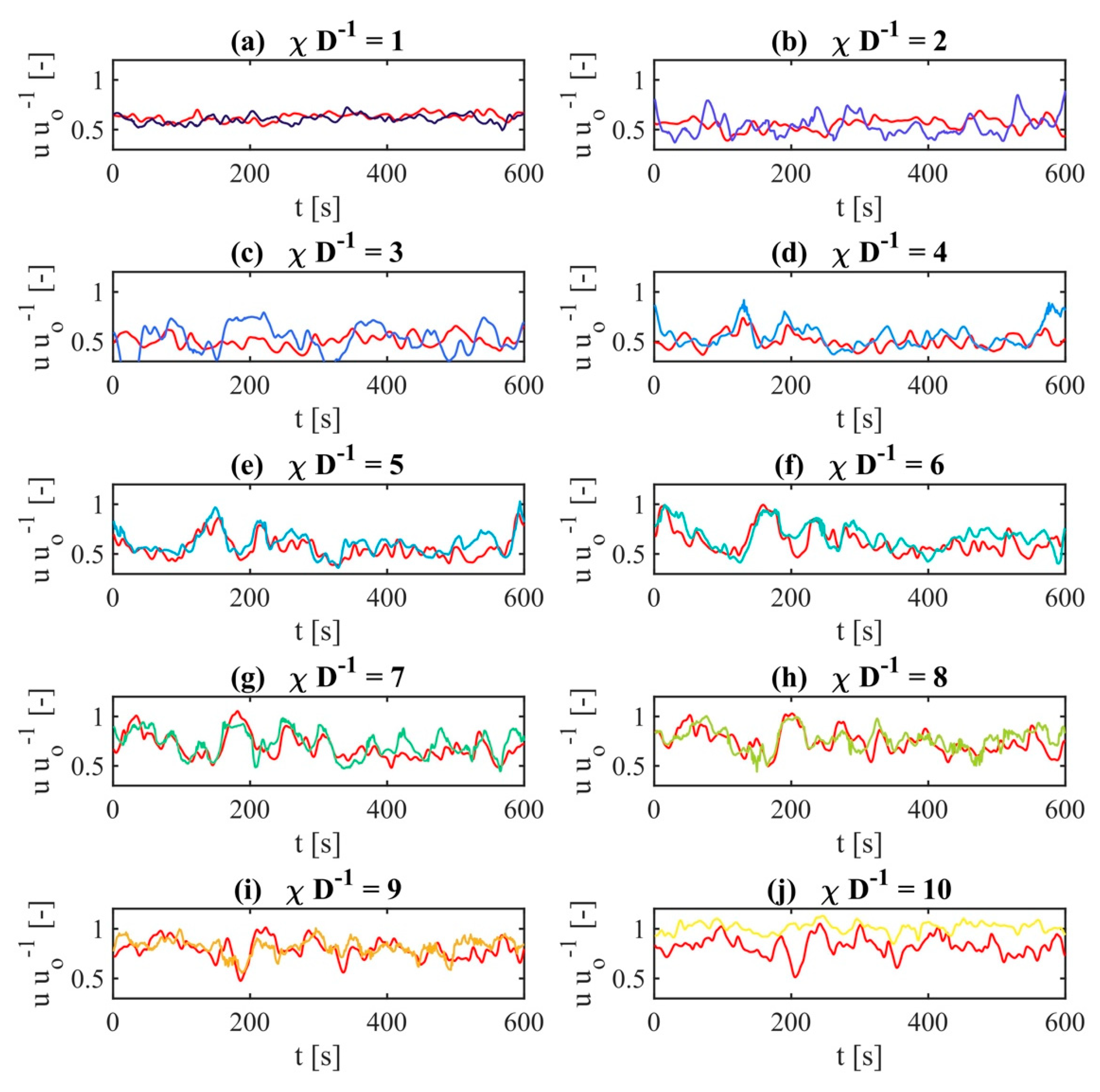
4.2.2. Dynamic Error Quantification

After examining the reconstruction errors in Section 4.2.1, we considered how far time-series dynamics could be mapped within the reconstructed wind field. We firstly used known methods to represent the time-series dynamics reconstruction quality and then presented an approach to quantify the dynamic errors.
To this end, we firstly considered cross-correlations of the original LES time series and reconstructed wind field for each point in space in Figure 13a. The correlation of different time series in the wake region was lower than that in the free flow surrounding it. Although the reconstructed wind field reached a nearly perfect correlation in the free stream, a minimum of 0.39 could be found in the wake at χ D 1   3 . For downstream distances of 4     χ D 1   9 , where the previously mentioned propagation errors were lower, we saw correlations greater than 0.65. Apparently, the linear correlation decrease relied on the wake velocity distribution (Figure 11b). This effect could be attributed to the decreased average velocity in the wake. Thus, fluctuation differences due to time-delayed meander events had a greater reducing effect on cross-correlation calculations than time-series data within free stream situations.
It was assumed that flow fluctuations, especially in the wake, were primarily responsible for fatigue loads; therefore, we conducted cross-correlations referring to mean value-adjusted fluctuations (subtraction of local velocity average) of the wind field in Figure 13b. The mean-adjusted free flow was only characterized by turbulence; thus, these areas showed a low correlation, as expected. In Figure 13b, we further detected that high correlation areas changed with increased downstream distance. Although a round wake shape could be clearly identified up to χ D 1   3 , collimated high-correlation areas were visible on the hub height center line for χ D 1   > 3 . For both Figure 13a,b, the boundary condition problem’s influence by propagation could be recognized at χ D 1   10 , as indicated by the lower correlation values.
To further evaluate the similarity of the reconstructed wind field and LES, we used an approach commonly known in the field of speech recognition. Because the cross-correlation considered dynamics of the largest possible time scale of the time series, small-scale signal shifts could not be individually considered. Figure 14 shows time-dependent velocity curves at different downstream distances along the center line of the reconstructed wind field and corresponding LES data (red). As shown in Figure 14d–i, the original and reconstructed time series showed similar behaviors in which individual peaks shifted in intensity and time. To describe the reconstruction quality of these individual peak events, we applied dynamic time warping (DTW), which dynamically stretches and compresses signals to minimize the Euclidean distance. Two information groups were generated using DTW. One part of the result was the mutual assignment of each data point of the reconstructed time series to a data point of the original time series. Figure 15a illustrates the allocation of velocity data for different downstream distances to the corresponding time index of the original time series. The graph could, thus, be interpreted as an assignment path for both signals. The dashed red diagonal line corresponds to the mapping of two identical signals. As the corresponding allocation paths shifted further from the diagonal, the displacements of single peak events became more pronounced within the time series. We calculated the average mutual time deviation ε Δ t of both time series by determining the average of the deviations of the time index of the allocated data points Δ t in Figure 15b.
We used the average time error ε Δ t ¯ magnitude as a measure of the dynamic reconstruction quality, which we illustrate for all points of the reconstructed wind field in vertical slices in Figure 16c. A smaller deviation indicated a more accurate temporal representation of peak events.
Because wind turbine load calculations showed a greater dependence on inflow variability and spectral representation than on a wind speed offset, we saw the mean temporal error ε Δ t ¯ as a pragmatic measure to represent the effects of different dynamics within the time series. The instantaneous temporal error of the reconstructed time series led to a different dynamic of the time series, thus leading to a spectral change in the wind speed. Further studies comparing load calculations of the reconstructed wind fields with those of the LES reference must first evaluate to what extent the mean temporal error can represent differences in time-series dynamics, and then determine to what extent which scalar is suitable for representing the allocation path.
As seen in the results above, the distribution of ε Δ t ¯ indicated an increased error in the near-wake area up to χ D 1 3 . From this distance on, the reconstruction quality improved along the center line, representing an average time error of ε Δ t ¯ 25   s for the total duration of 600 s within the wake region.
The second result of the DTW was the time-series Euclidean distance based on the allocated data. The distance of the unadjusted time series in Figure 16a is shown in contrast to that of the adjusted time series in Figure 16b. At 4     χ D 1   9 , improvements in velocity error correlated with regions with small average temporal errors. The considerably reduced Euclidean distance seen in the comparison showed the remaining error of the differences in the amplitudes of the new allocated peak events. The average wind speed error in Figure 11c could, thus, be divided into its constituent components. One part was an offset and the other was due to different dynamics. With the DTW, we could quantify both components and evaluate the reconstruction. Therefore, we saw this method as a good indicator for evaluating the quality of peak event reconstructions. A smaller average time error (Figure 16c) indicated more precise representation of the wake dynamics by wake tracking. Additionally, smaller remaining Euclidean distances (Figure 16b) demonstrated a more accurately determined wake deficit in the MFoR, which in turn depended on wake dynamics determination.

5. Discussion

In this section, we discuss the introduced method for reconstructing 3D1C wake wind fields from LiDAR measurements and its results.
One significant difficulty with designing a wake reconstruction method is the limited possibility of verification due to a lack of measurement methods needed for a holistic validation. A limited validation of the proposed reconstruction method could still be conducted in full-field measurements. If the corresponding reference data from one or more anemometers in the wake region are available, an evaluation can be performed based on the comparison of statistics or application of DTW, which is a comparison of time series. Nevertheless, the gap of the 3D1C wind speed wake measurements leads to an assumption that simplifications considered in the LiDAR simulation can represent significant full-field LiDAR measurement characteristics. With the way the LiDAR simulator is used here, only step-and-stare LiDAR measurements have direct comparability; however, in application, most scanning measurements are conducted on the fly. Backscattering accumulates during scanning, which leads to additional volume averaging in the scanning direction. Because we cannot reproduce non-linear signal processing within the real LiDAR data, we accommodate this effect using the posterior averaging of wind speed data within the volumetric deficit calculation in the MFoR.
When using physical or simulated long-range LiDAR data, one-dimensional measurements assume vertical and lateral velocity component homogeneity to process them without requiring an additional flow solver for the main wind velocity component. In the near-wake range, the rotor causes complex flows that cannot be mapped using this assumption. As shown in Figure 11c, this inaccuracy does not necessarily lead to significant mean wind speed errors; however, it contributes to the mapping of the standard deviation error, as can be seen in Figure 12c for χ D 1   3 .
We accept a further significant assumption when calculating the volumetric wind velocity deficit in the MFoR. Because of the limited scanning speeds of long-range LiDARs, it is not feasible to volumetrically measure wakes on appropriate time scales. So far, only center line cross-trajectories were analyzed; thus, we introduce the conditional rotational wake symmetry assumption. Although the conditional rotation presented here, which is based on four different quadrants, exceeds a simple axial/point symmetry, deficit shape changes in the diagonal direction must be modeled in further applications. The influence of wind veer on the wake deficit’s horizontal distortion in the vertical direction was marginal in this study, and it was compensated for by using a linear displacement approach similar to the advection assumption of the DWM. Because the differences only became apparent in the third decimal place, it is only stated here in the discussion. We find it reasonable to conduct further studies in which X-shaped measurement trajectories are used as a measurement pattern to better capture the potential veer. Studies with corresponding LES wind fields show the extent to which this effect can be achieved with significant height-dependent wind direction differences.
The last assumptions we consider are those of reconstruction. The method shown here can be interpreted as an adaptation of the DWM model based on LiDAR measurements. Air parcel advection speed and tracking position are not calculated using a point time series, but rather recreated based on the tracked dynamics from LiDAR scans. Even if the introduced shape and intensity dynamics may represent a more realistic deficit dynamics behavior, the assumption that the velocity deficit can be seen as a homogeneous structure on small time scales can only be justified to certain downstream distances.
Despite the many simplifications used, we are encouraged in our assumptions to derive and determine wake dynamics using long-range LiDAR data, because of the good representativeness of the reconstructed wind field shown. The extent to which the reconstructed wake wind fields can produce realistic turbine loads and how turbulence characteristics on time scales smaller than the temporal resolution of the measurements are satisfied by this approach will be discussed in the future.

6. Conclusions

This paper presented a method for reconstructing spatially and temporally high-resolution 3D1C wind-turbine wake wind fields from volumetric long-range LiDAR data. The method’s evaluation used a numerical LiDAR simulator that calculates 1D LOS velocities from an LES wake wind field. The scan parameters used were taken from a real nacelle-based measurement campaign using two LiDARs, and extended by a parameter study of how far different scan speeds influence wake dynamics representation. Eight different scanning speeds were evaluated for each planar horizontal and vertical measurement. To determine the wake dynamics, the temporal shift within each LiDAR scan was firstly corrected and then mutually synchronized. For this purpose, we propagated LiDAR measurements using a space–time conversion approach to retrospectively improve the temporal resolution to a sub-measurement scale. From this high-resolution temporal data, we derived the wake dynamics for position, shape, and intensity by using a Gaussian curve fitting. We calculated the volumetric wake deficit in the MFoR, which we displaced and scaled with the tracked dynamics to reconstruct the dynamic wake behavior. Finally, we superimposed a synthetic turbulent wind field that was scaled based on the tracked wake dynamics.
In the comparison of the reconstructed and original LES wind fields, multiple results could be observed for horizontal and vertical scanning velocity combinations. Although an apparent minimum of 2.3% of the ambient wind speed could be found for the average wind speed reconstruction, the standard deviation followed an exponential trend of horizontal and vertical angular velocity combinations. The maximum accuracy of the standard deviation reconstruction was 0.18–0.3%. We showed that either the averaged wind speeds or their standard deviations could be accurately mapped.
In particular, the good results of dynamic wake behavior reconstruction indicate that wake characterization and modeling using long-range LiDAR measurements that are not optimally resolved in time are possible if the space–time conversion used here is applied.
With ongoing research in wind-field propagation, a more precise determination of the wake behavior is possible. Furthermore, increased wake tracking accuracy will directly improve the reconstruction quality and the understanding of wake behavior.

Supplementary Materials

The following are available online at https://www.mdpi.com/2072-4292/11/22/2665/s1: Video S1: Propagation and wake tracking results of horizontal wind speed data for variable angular velocities; Video S2: Propagation and wake tracking results of vertical wind speed data for variable angular velocities; Video S3: Comparison of the reconstructed wake wind field with the LES reference wake wind field.

Author Contributions

This study was conducted as a part of H.B.’s doctoral studies, supervised by M.K., H.B. conducted the research and wrote the paper. M.K. supervised the research, contributed to the structure of the paper, and performed review and editing.

Funding

This work was partially funded by the Federal Ministry for Economic Affairs and Energy (BMWi) according to a resolution given by the German Federal Parliament (project CompactWind, FKZ 0325492B) and in the scope of the ventus efficiens project (ZN3092), through the funding initiative Niedersächsisches Vorab of the Ministry for Science and Culture of Lower Saxony.

Acknowledgments

We are also grateful to Juan José Trujillo for valuable discussion. We thank Davide Trabucchi for the implementation of the LiDAR simulator LiXIM. We thank Andreas Rott for the idea and the closure of the wind-field propagation. We thank Mehdi Vali for performing the LES simulation of the wake wind field. All colleagues are/were affiliated to the research group Wind Energy Systems at the University of Oldenburg.

Conflicts of Interest

The authors declare no conflict of interest.

Abbreviations

The following abbreviations are used in this manuscript:
ABLAtmospheric boundary layer
ACLActuator line approach
ADEArtificial data extension
CFDComputational fluid dynamics
DTWDynamic time warping
DWMDynamic wake meandering
EDPmExtended disk particle model
FFoRFixed frame of reference
LESLarge-eddy simulation
LiDARLight detection and ranging
LOSLine-of-sight
MFoRMeandering frame of reference
PALMParallelized large-eddy simulation model
PPIPlan position indicator
RHIRange height indicator
SCADASupervisory control and data acquisition
VDVolumetric deficit

Formula Symbols

α γ , α ζ Wake deficit intensity within the Gaussian fitting
β γ , β ζ Ambient longitudinal wind speed level within the Gaussian fitting
δ F F o R , δ V D F F o R Instantaneous wake velocity deficit in the fixed frame of reference
δ F F o R ¯ Averaged wake velocity deficit in the fixed frame of reference
δ M F o R Instantaneous wake velocity deficit in the meandering frame of reference
δ M F o R ¯ , δ VD MFoR ¯ Averaged wake velocity deficit in the meandering frame of reference
Δ ϕ , Δ θ Total opening angle of PPI and RHI scans
ε u ¯ Mean wind speed reconstruction error
ε σ u Standard deviation reconstruction error
η m Measurement time efficiency
θ Elevation angle
θ Difference angle of the vertical wind direction ( Θ ) and elevation angle ( θ )
Θ Vertical wind direction
ϑ a c c Measurement accumulation time
λ 
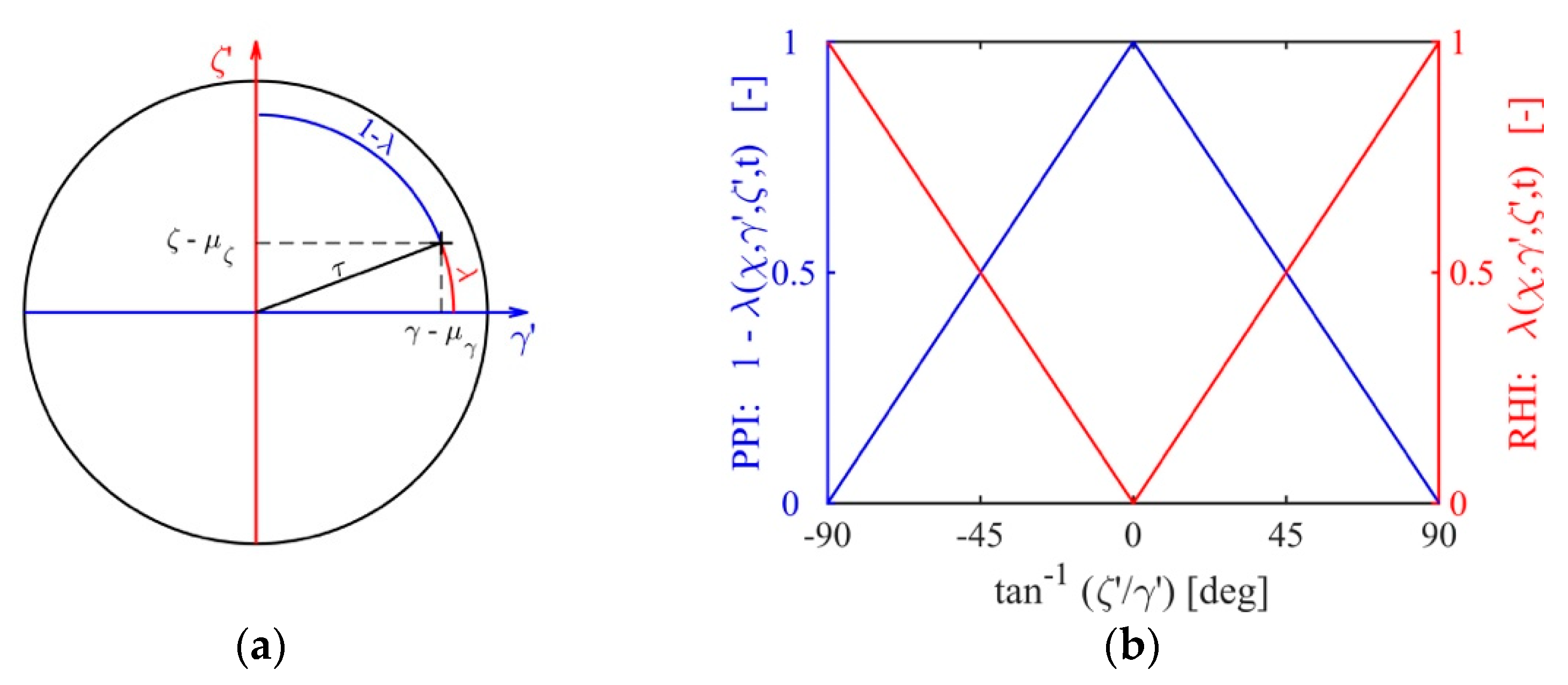
Rotational weighting function
μ γ , μ ζ Wake center position within the Gaussian fitting
υ ^ L O S Radial LiDAR velocity
σ γ , σ ζ Wake width within the Gaussian fitting
σ VD MFoR Standard deviation of the wind speed in the wake in the meandering frame of reference
τ Radial distance within the γ ζ coordinate system
ϕ Azimuth angle
Φ Horizontal wind direction
ϕ Difference angle of the horizontal wind direction ( Φ ) and azimuth angle ( ϕ )
ω ϕ , ω θ Angular scan velocity
χ , γ , ζ Fixed reference frame coordinate system in the turbine ground point
χ , γ , ζ Meandering reference frame coordinate system
D Rotor diameter
f s Measurement frequency
h HH Wind turbine hub height
I 0 Ambient turbulence intensity in the fixed frame of reference
I VD MFoR Turbulence intensity in the meandering frame of reference
n p n t Number of measurement points within a scan
n ϕ , n θ Number of angular measurements per scan
Ν ϕ , Ν θ Number of scans per time interval
r γ , r ζ Radial position in transversal in-plane direction within the Gaussian fitting
ϕ ,   θ Angular resolution of PPI and RHI scans
s I 0 MFoR Turbulence intensity scaling factor in the meandering frame of reference
s γ Horizontal spatial deficit shape scaling factor
s ζ Horizontal spatial deficit shape scaling factor
s δ Velocity deficit intensity scaling factor
tPoint in time
t r Reset time
TSet of all discrete measurement points in time t
Τ ϕ , Τ θ Scan duration
u o Instantaneous ambient longitudinal wind speed
u o ¯ Average ambient longitudinal wind speed
u a Instantaneous ambient longitudinal wind speed of synthetic wind field
u a ¯ Average ambient longitudinal wind speed of synthetic wind field
u fit , PPI Gaussian-shaped wake wind speed profile within a PPI scan
u fit , RHI Gaussian-shaped wake wind speed profile within a PPI scan
u LES LES wind speed
u VD MFoR ¯ Averaged wind speed of wake in the meandering frame of reference
u PPI PPI wind speed
u P P I PPI wind speed
u R H I RHI wind speed
u RC Instantaneous ambient longitudinal wind speed of reconstructed wind field
u r o t Rotated and weighted wind speed combination of RHI and PPI in the MFoR
u t Turbulent component of u a
v 0 ¯ Average ambient lateral wind speed
w 0 ¯ Average ambient vertical wind speed

Appendix A

Figure A1. Visualization of the tracked vertical wake center μ ζ in the FFoR as a function of time t and downstream distance χ : (a–h) the effect of different angular velocities on tracking; (i) μ ζ based on LES data.
Remotesensing 11 02665 g0a1

References

  1. Crespo, A.; Hernandez, J.; Frandsen, S. Survey of modelling methods for wind turbine wakes and wind farms. Wind Energy 1999, 2, 1–24. [Google Scholar] [CrossRef]
  2. Vermeer, L.; Sørensen, J.N.; Crespo, A. Wind turbine wake aerodynamics. Prog. Aerosp. Sci. 2003, 39, 467–510. [Google Scholar] [CrossRef]
  3. Kelley, N.D.; Osgood, R.M.; Bialasiewicz, J.T.; Jakubowski, A. Using wavelet analysis to assess turbulence/rotor interactions. Wind Energy 2000, 3, 121–134. [Google Scholar] [CrossRef]
  4. Hand, M. Mitigation of Wind Turbine/Vortex Interaction Using Disturbance Accommodating Control. Ph.D. Thesis, National Renewable Energy Laboratory, Golden, CO, USA, December 2003. [Google Scholar] [CrossRef]
  5. Ainslie, J.F. Calculating the flowfield in the wake of wind turbines. J. Wind Eng. Ind. Aerodyn. 1988, 27, 213–224. [Google Scholar] [CrossRef]
  6. Jensen, N.O. A Note on Wind Generator Interaction; Tech. Rep. Risø-M-2411(EN); Risø National Laboratory: Roskilde, Denmark, 1983. [Google Scholar]
  7. Frandsen, S.; Barthelmie, R.; Pryor, S.; Rathmann, O.; Larsen, S.; Højstrup, J.; Thøgersen, M. Analytical modelling of wind speed deficit in large offshore wind farms. Wind Energy 2006, 9, 39–53. [Google Scholar] [CrossRef]
  8. Trujillo, J.J. Large Scale Dynamics of Wind Turbine Wakes. Ph.D. Thesis, University of Oldenburg, Oldenburg, Germany, 2018. [Google Scholar]
  9. Larsen, G.C.; Madsen, H.A.; Thomsen, K.; Larsen, T.J. Wake meandering: A pragmatic approach. Wind Energy 2008, 11, 377–395. [Google Scholar] [CrossRef]
  10. Foti, D.; Yang, X.; Guala, M.; Sotiropoulos, F. Wake meandering statistics of a model wind turbine: Insights gained by large eddy simulations. Phys. Rev. Fluids 2016, 1, 4407. [Google Scholar] [CrossRef]
  11. Aitken, M.L.; Kosović, B.; Mirocha, J.D.; Lundquist, J.K. Large eddy simulation of wind turbine wake dynamics in the stable boundary layer using the Weather Research and Forecasting Model. J. Renew. Sustain. Energy 2014, 6, 5111. [Google Scholar] [CrossRef]
  12. Bromm, M.; Vollmer, L.; Kühn, M. Numerical investigation of wind turbine wake development in directionally sheared inflow. Wind Energy 2017, 20, 381–395. [Google Scholar] [CrossRef]
  13. Porté-Agel, F.; Wu, Y.-T.; Lu, H.; Conzemius, R.J. Large-eddy simulation of atmospheric boundary layer flow through wind turbines and wind farms. J. Wind Eng. Ind. Aerodyn. 2011, 99, 154–168. [Google Scholar] [CrossRef]
  14. Sturge, D.; Sobotta, D.; Howell, R.; While, A.; Lou, J. A hybrid actuator disc–Full rotor CFD methodology for modelling the effects of wind turbine wake interactions on performance. Renew. Energy 2015, 80, 525–537. [Google Scholar] [CrossRef]
  15. Vijayakumar, G.; Brasseur, J.; Lavely, A.W.; Jayaraman, B.; Craven, B. In Interaction of atmospheric turbulence with blade boundary layer dynamics on a 5MW wind turbine using blade-boundary-layer-resolved CFD with hybrid URANS-LES. In Proceedings of the 34th Wind Energy Symp, San Diego, CA, USA, 4–8 January 2016; p. 0521. [Google Scholar] [CrossRef]
  16. Schmidt, B.; King, J.; Larsen, G.C.; Larsen, T.J. Load validation and comparison versus certification approaches of the risø dynamic wake meandering model implementation in GH bladed. In Proceedings of the EWEA Annual Event 2011, Brussels, Belgium, 14–17 March 2011; pp. 249–254. [Google Scholar]
  17. Larsen, G.C.; Ott, S.; Larsen, T.J.; Hansen, K.; Chougule, A. In Improved Modelling of Fatigue Loads in Wind Farms under Non-Neutral ABL Stability Conditions; (Journal of Physics: Conference Series); IOP Publishing: Bristol, UK, 2018; p. 072013. [Google Scholar] [CrossRef]
  18. Käsler, Y.; Rahm, S.; Simmet, R.; Kühn, M. Wake measurements of a multi-MW wind turbine with coherent long-range pulsed Doppler wind lidar. J. Atmos. Ocean. Technol. 2010, 27, 1529–1532. [Google Scholar] [CrossRef]
  19. Aitken, M.L.; Lundquist, J.K. Utility-scale wind turbine wake characterization using nacelle-based long-range scanning lidar. J. Atmos. Ocean. Technol. 2014, 31, 1529–1539. [Google Scholar] [CrossRef]
  20. Bromm, M.; Rott, A.; Beck, H.; Vollmer, L.; Steinfeld, G.; Kühn, M. Field investigation on the influence of yaw misalignment on the propagation of wind turbine wakes. Wind Energy 2018, 21, 1011–1028. [Google Scholar] [CrossRef]
  21. Aubrun, S.; Garcia, E.T.; Boquet, M.; Coupiac, O.; Girard, N. In Statistical Analysis of A Field Database to Study Stability Effects on Wind Turbine Wake Properties; (Journal of Physics: Conference Series); IOP Publishing: Bristol, UK, 2018; p. 072047. [Google Scholar] [CrossRef]
  22. Beck, H.; Kühn, M. Temporal up-sampling of planar long-range doppler LiDAR wind speed measurements using space-time conversion. Remote Sens. 2019, 11, 867. [Google Scholar] [CrossRef]
  23. Carbajo Fuertes, F.; Porté-Agel, F. Using a virtual Lidar approach to assess the accuracy of the volumetric reconstruction of a wind turbine wake. Remote Sens. 2018, 10, 721. [Google Scholar] [CrossRef]
  24. Borraccino, A.; Schlipf, D.; Haizmann, F.; Wagner, R. Wind field reconstruction from nacelle-mounted lidars short range measurements. Wind Energy Sci. 2017, 2, 269–283. [Google Scholar] [CrossRef]
  25. Kapp, S.; Kühn, M. In A Five-Parameter Wind Field Estimation Method Based on Spherical Upwind Lidar Measurements; (Journal of Physics: Conference Series); IOP Publishing: Bristol, UK, 2014; p. 012112. [Google Scholar] [CrossRef]
  26. Towers, P.; Jones, B.L. Real-time wind field reconstruction from LiDAR measurements using a dynamic wind model and state estimation. Wind Energy 2016, 19, 133–150. [Google Scholar] [CrossRef]
  27. Iungo, G.V.; Porté-Agel, F. Volumetric lidar scanning of wind turbine wakes under convective and neutral atmospheric stability regimes. J. Atmos. Ocean. Technol. 2014, 31, 2035–2048. [Google Scholar] [CrossRef]
  28. Van Dooren, M.; Trabucchi, D.; Kühn, M. A methodology for the reconstruction of 2D horizontal wind fields of wind turbine wakes based on dual-Doppler lidar measurements. Remote Sens. 2016, 8, 809. [Google Scholar] [CrossRef]
  29. Raasch, S.; Schröter, M. PALM–A large-eddy simulation model performing on massively parallel computers. Meteorol. Z. 2001, 10, 363–372. [Google Scholar] [CrossRef]
  30. Troldborg, N. Actuator Line Modeling of Wind Turbine Wakes. Ph.D. Thesis, Technical University of Denmark, Lyngby, Denmark, June 2008. [Google Scholar]
  31. Jonkman, J.; Butterfield, S.; Musial, W.; Scott, G. Definition of a 5-MW Reference Wind Turbine for Offshore System Development; National Renewable Energy Laboratory (NREL): Golden, CO, USA, 2009.
  32. Deardorff, J. Stratocumulus-capped mixed layers derived from a three-dimensional model. Bound. -Layer Meteorol. 1980, 18, 495–527. [Google Scholar] [CrossRef]
  33. Trabucchi, D.; Trujillo, J.; Steinfeld, G.; Schneemann, J.; Machtaa, M.; Cariou, J.; Kühn, M. In Numerical Assessment of Performance of Lidar Wind Scanners for Wake Measurements; EWEA Annual Event 2011, European Wind Energy Association (EWEA): Brussels, Belgium, 2011. [Google Scholar]
  34. Sibson, R. A brief description of natural neighbour interpolation. In Interpreting Multivariate Data; Wiley: New York, NY, USA, 1981; pp. 21–36. [Google Scholar] [CrossRef]
  35. Trujillo, J.J.; Bingöl, F.; Larsen, G.C.; Mann, J.; Kühn, M. Light detection and ranging measurements of wake dynamics. Part II: Two-dimensional scanning. Wind Energy 2011, 14, 61–75. [Google Scholar] [CrossRef]
  36. Brent, R.P. Algorithms for Minimization without Derivatives; Courier Corporation: North Chelmsford, MA, USA, 1973; pp. 61–167. [Google Scholar]
Figure 1. Illustration of cross-measurement trajectories, coordinate system, and velocity components. Measurement trajectories comprise one repeating horizontal plan position indicator (PPI) scan (dark blue) and one repeating vertical range height indicator (RHI) scan (shown in pink). The wake volume is indicated in light blue.
Remotesensing 11 02665 g001
Figure 2. Schematic representation of the model assumptions within the reconstruction. Different half axes of the ellipses indicate different scaling of the wake velocity deficit in the horizontal and vertical directions, whereas the colors correspond to scaled wake velocity deficit intensities for one point in time: (a) side view; (b) top view; (c) perspective view.
Remotesensing 11 02665 g002
Figure 3. Illustration of the time series of the PPI scan azimuth angle, including a visualization of the temporal alignment at time t . Dark-blue lines indicate light detection and ranging (LiDAR) measurements, light-blue lines indicate propagated scans, green lines indicate the measurement reset trajectory during the reset time ( t r ), and the red line represents temporal interpolation at time t . The example shows 11 interpolation steps between two consecutive scans [22].
Remotesensing 11 02665 g003
Figure 4. Application of Gaussian fitting to a LiDAR measurement of a wake in a downstream distance of five dimensions (5D). μ indicates the wake center position (light blue), σ represents the Gaussian wake width (turquoise), α denotes the intensity of the deficit (yellow), and β labels the ambient longitudinal wind speed levels (green).
Remotesensing 11 02665 g004
Figure 5. Illustration of the rotational assumption of the wake wind field calculation in the meandering frame of reference (MFoR). (a) Geometric relationship of PPI (blue) and RHI scans (red) in the MFoR, and (b) weighting of PPI (blue) and RHI (red) wind speed data dependent on positions γ and ζ .
Remotesensing 11 02665 g005
Figure 6. Visualization of tracked horizontal wake center μ γ in the fixed reference frame (For) for time t and downstream distance χ . (a–h) Effects of different angular velocities on tracking; (i) μ γ based on large-eddy simulation (LES) data.
Remotesensing 11 02665 g006
Figure 7. Illustration of the artificial data extension: (a) wind speed-normalized PPI scan; (b) results of the method. The scan trajectory outline is marked in red.
Remotesensing 11 02665 g007
Figure 8. Mean value and standard deviation of wake tracking results for propagated PPI data: (a) horizontal wake center of original data; (b) horizontal wake center based on artificial data extension; (c) horizontal wake width of original data; (d) horizontal wake width based on artificial data extension.
Remotesensing 11 02665 g008
Figure 9. Mean value and standard deviation of wake tracking results for propagated RHI data: (a) vertical wake center of original data; (b) vertical wake center based on artificial data extension; (c) vertical wake width of original data; (d) vertical wake width based on artificial data extension.
Remotesensing 11 02665 g009
Figure 10. Error visualization of the reconstructed wind field based on the LES wake wind field: (a) average wind speed error; (b) standard deviation error; (c) a combination of average and standard deviation error. All three errors are related to combinations of the vertical and horizontal scanning angular velocities ω θ and ω ϕ .
Remotesensing 11 02665 g010
Figure 11. Normalized wind speed component u of (a) the LES wake wind field, (b) reconstructed wind field with ω ϕ   =   4 ° / s and ω θ   =   19.11 ° / s , and (c) the differences between the LES and reconstructed wind fields.
Remotesensing 11 02665 g011
Figure 12. Standard deviation of the normalized wind speed component u of (a) the LES wake wind field, (b) the reconstructed wind field with ω ϕ   =   4 ° / s and ω θ   =   19.11 ° / s , and (c) differences between the LES and reconstructed wind fields.
Remotesensing 11 02665 g012
Figure 13. Correlation of the LES wake wind field time series with reconstructed wind field time series: (a) correlation result based on the time series; (b) correlation result based on average-adjusted time series.
Remotesensing 11 02665 g013
Figure 14. Direct comparison of wind speed time series of the LES wake wind field (red) and the reconstructed wind field for different downstream distances along the hub height center line. Different colors refer to corresponding downstream distances.
Remotesensing 11 02665 g014
Figure 15. Results of dynamic time warping application on the LES wake wind field time series and reconstructed time series: (a) allocation paths of time series, and (b) the resulting temporal errors of peak events along the hub height center line for different downstream distances.
Remotesensing 11 02665 g015
Figure 16. (a) Visualization of the Euclidian distance between the time series of the LES and reconstructed wind field; (b) Euclidian distance of the new allocated time series of the LES and the reconstructed wind field after applying dynamic time warping; (c) resulting average time error of the LES and reconstructed time series by application of dynamic time warping.
Remotesensing 11 02665 g016
Table 1. Simulated light detection and ranging (LiDAR) trajectories of cross-measurements for a time interval of 600 s and 180 radial measurement points in the range of 0–1260 m.
ω ϕ ,
ω θ
Δ ϕ ,
Δ θ
Ν ϕ ,
Ν θ
n p n t n ϕ ,
n θ
ϕ   ,
θ
Τ ϕ
Τ θ
f s η m
1°/s40°1536,0002000.2°40.0 s0.024 Hz97.2%
2°/s40°2918,0001000.4°20.0 s0.047 Hz94.2%
4°/s40°549000500.8°10.0 s0.089 Hz89.2%
8°/s40°974500251.6°5.0 s0.161 Hz80.6%
12°/s40°1332880162.5°3.3 s0.221 Hz73.4%
19.11°/s40°1831800104.0°2.1 s0.303 Hz63.4%
26.22°/s40°221126075.7°1.5 s0.370 Hz55.8%
33.33°/s40°250108066.7°1.2 s0.417 Hz50.0%

