Article

Decomposing the Long-term Variation in Population Exposure to Outdoor PM2.5 in the Greater Bay Area of China Using Satellite Observations

1
Division of Environment and Sustainability, the Hong Kong University of Science and Technology, Hong Kong, China
2
Department of Civil and Environmental Engineering, the Hong Kong University of Science and Technology, Hong Kong, China
3
Department of Mathematics, the Hong Kong University of Science and Technology, Hong Kong, China
4
Shanghai Meteorological Service, Shanghai 200030, China
5
Department of Atmospheric and Oceanic Sciences, School of Physics, Peking University, Beijing 100871, China
6
State Key Laboratory of Geological Processes and Mineral Resources, China University of Geosciences, Wuhan 430074, China
*
Author to whom correspondence should be addressed.
Remote Sens. 2019, 11(22), 2646; https://doi.org/10.3390/rs11222646
Submission received: 16 October 2019 / Revised: 8 November 2019 / Accepted: 11 November 2019 / Published: 13 November 2019
(This article belongs to the Special Issue Urban Air Quality Monitoring using Remote Sensing)

Abstract

:
The Greater Bay Area (GBA) of China is experiencing a high level of exposure to outdoor PM2.5 pollution. The variations in the exposure level are determined by spatiotemporal variations in the PM2.5 concentration and population. To better guide public policies that aim to reduce the population exposure level, it is essential to explicitly decompose and assess the impacts of different factors. This study took advantage of high-resolution satellite observations to characterize the long-term variations in population exposure to outdoor PM2.5 for cities in the GBA region during the three most-recent Five-Year Plan (FYP) periods (2001–2015). A new decomposition method was then used to assess the impact of PM2.5 variations and demographic changes on the exposure variation. Within the decomposition framework, an index of pollution-population-coincidence–induced PM2.5 exposure (PPCE) was introduced to characterize the interaction of PM2.5 and the population distribution. The results showed that the 15-year average PPCE levels in all cities were positive (e.g., 6 µg/m3 in Guangzhou), suggesting that unfavorable city planning had led to people dwelling in polluted areas. An analyses of the spatial differences in PM2.5 changes showed that urban areas experienced a greater decrease in PM2.5 concentration than did rural areas in most cities during the 11th (2006–2010) and 12th (2011–2015) FYP periods. These spatial differences in PM2.5 changes reduced the PPCE levels of these cities and thus reduced the exposure levels (by as much as -0.58 µg/m3/year). The population migration resulting from rapid urbanization, however, increased the PPCE and exposure levels (by as much as 0.18 µg/m3/year) in most cities during the three FYP periods considered. Dongguan was a special case in that the demographic change reduced the exposure level because of its rapid development of residential areas in cleaner regions adjacent to Shenzhen. The exposure levels in all cities remained high because of the high mean PM2.5 concentrations and their positive PPCE. To better protect public health, control efforts should target densely populated areas and city planning should locate more people in cleaner areas.

Graphical Abstract

1. Introduction

Long-term exposure to outdoor particulate matter with an aerodynamic diameter of <2.5 μm (PM2.5) is associated with a range of adverse health effects [1,2,3,4,5]. The level of population exposure to outdoor PM2.5 in China is much higher than that in the U.S. or Europe [6]. As one of the major city clusters in China, the Pearl River Delta (PRD) region is exposed to a high level of PM2.5 pollution [7]. The population-weighted mean PM2.5 concentrations have been extensively used by researchers as an indicator of the population exposure level [8,9,10,11,12,13,14,15]. It is estimated by averaging the ambient PM2.5 concentration associated with each individual within the study region. Burnett et al. [16] assessed the global population exposure to outdoor PM2.5 in 2015 and concluded that the population-weighted mean PM2.5 concentrations varied from the lowest levels in Canada/U.S. (7.9 μg/m3) to the highest levels in China (57.5 μg/m3) and India (74.0 μg/m3). Using satellite-derived PM2.5 data, Lin et al. [17] estimated the population-weighted mean PM2.5 concentration to be 43.9 μg/m3 in the PRD region from 2000 to 2014. In addition, their results showed that 84.0% of the population lived in areas with PM2.5 concentrations that exceeded the World Health Organization (WHO) Interim Target 1 (IT-1) or the Chinese National Ambient Air Quality Standard (NAAQS), both of which are 35 µg/m3. In February 2019, the “Outline Development Plan for Guangdong-Hong Kong-Macao Greater Bay Area” (the Greater Bay Area (GBA) Plan) was promulgated, which emphasized green development in this region. The regulation of pollutant emissions was tightened to further alleviate air pollution.
The variations in the mean PM2.5 concentration level directly affect a population’s exposure level in any given city. During the past decade, the governments of Guangdong Province and Hong Kong promulgated a series of control measures to reduce the PM2.5 concentration [18]. Using satellite observations, Ma et al. [19] showed that the mean PM2.5 concentration in the GBA region remained relatively constant from 2004 to 2007 and decreased from 2008 to 2013. Another study reported that all cities in the GBA region experienced an increasing mean PM2.5 concentration during the 10th Five-Year Plan (FYP) period (2001–2005) and a decreasing mean PM2.5 concentration during the 11th (2006–2010) and 12th (2011–2015) FYP periods [20].
A decrease in the mean PM2.5 concentration is not necessarily associated with a decreasing population exposure level for the city if the PM2.5 concentrations decrease in vast rural areas but increase in densely populated urban areas. The spatial differences in PM2.5 changes therefore play an important role in exposure management [21]. Ideally, control efforts to reduce the PM2.5 concentration should target densely populated urban areas. Lin et al. [22] assessed the differences in PM2.5 variations between urban and rural areas for Chinese provinces, and they showed that the urban areas in the GBA region experienced a greater decrease in the PM2.5 concentration than did rural areas during the 11th and 12th FYP periods. This type of spatial difference in PM2.5 change assists a region to reduce its population exposure level.
Rapid urbanization typically leads to population migration into large urban areas. As reported by the Chinese statistical yearbook, the urban population in Guangdong Province increased from 47.5 million (55% of total population) in 2000 to 74.5 million (69% of total population) in 2015 (http://www.stats.gov.cn/tjsj/ndsj/). As urban areas are typically highly polluted, the migration of people to the urban areas in the GBA region during the past decade tended to increase its overall population exposure level. Ideally, demographic changes can reduce the exposure level if city planners relocate the population away from polluted areas. Further scientific and quantitative investigation of the impact of demographic change is needed.
The variations in the population exposure level are therefore determined by changes in the mean PM2.5 concentration, spatial differences in PM2.5 change and demographic changes. The level of population exposure to PM2.5 for a city decreases if: (1) the mean PM2.5 concentration declines, (2) urban areas experience a greater reduction of PM2.5 concentration than rural areas, or (3) city planners relocate people away from polluted areas. To better guide public policies that aim to reduce exposure levels, it is essential to explicitly decompose and assess the impact of different factors.
Traditional studies have used ground-based networks to monitor the PM2.5 concentration. However, such monitoring in China is much more limited than in developed countries [23]. Satellite remote sensing is an important step toward filling this data gap [24,25,26]. This study took advantage of high-resolution satellite observations to characterize long-term variations in human exposure to PM2.5 for cities in the GBA region during the three most-recent FYP periods (2001–2015). A new decomposition method was then used to assess the impact of PM2.5 variations and demographic changes on the exposure variation. Finally, suggestions for future environmental policies and urbanization planning were developed.

2. Data

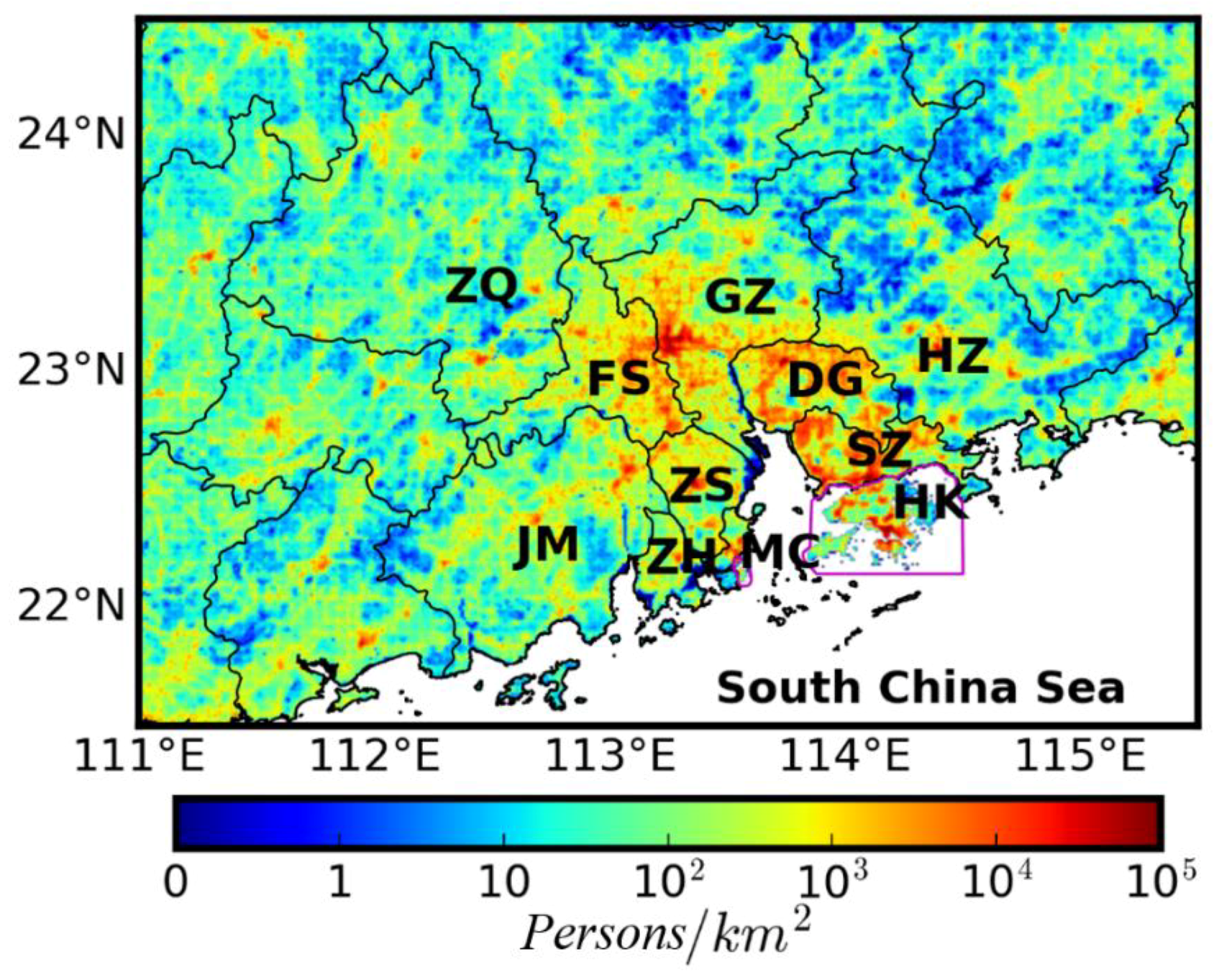
2.1. Population Density

The GBA region of China contains nine major cities in Guangdong Province [Guangzhou (GZ), Shenzhen (SZ), Zhuhai (ZH), Dongguan (DG), Foshan (FS), Zhongshan (ZS), Zhaoqing (ZQ), Jiangmen (JM) and Huizhou (HZ)]. Guangzhou is the capital city of Guangdong Province. Shenzhen and Zhuhai are two special economic zones of China. The GBA region also contains two special administrative zones of China [i.e., Hong Kong (HK) and Macau (MC)]. All eleven administrative regions as cities were considered.
The yearly population density data was obtained at a spatial resolution of 1 km for the GBA region for 2001 and 2015 from the LandScan population database (http://web.ornl.gov/sci/landscan/). LandScan population data was constructed with the use of spatial data and imagery analyses to disaggregate census counts within administrative boundaries. A linear interpolation method was then applied to derive population densities for other years of the study period. The year- and city-specific gross population data were obtained from 2001 to 2015 from local statistical yearbooks (http://www.gdstats.gov.cn/). The LandScan-derived population data were adjusted by year- and city-specific factors to match the gross populations from the statistical yearbooks. Figure 1 shows the spatial distribution of the 15-year mean of population density in the GBA region. The population densities exceeded 103 persons/km2 in urban areas of the GBA region.

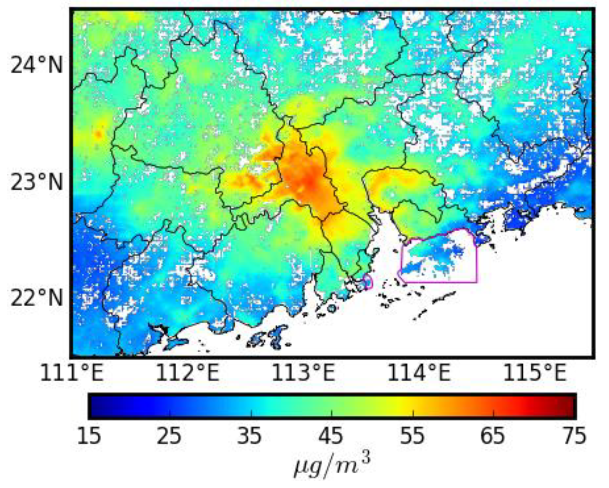
2.2. Satellite-Derived PM2.5

A high-resolution satellite-based PM2.5 dataset was taken advantage of to characterize the long-term variations in the PM2.5 concentration in the GBA region (http://envf.ust.hk/dataview/aod2pm/current). The algorithm was first used to build aerosol optical depth (AOD) data at a spatial resolution of 0.01° × 0.01° using spectral data from the two Moderate Resolution Imaging Spectroradiometer (MODIS) instruments aboard the Terra and Aqua satellites [27]. The verification of the satellite-retrieved AOD against the ground-based sunphotometer observations showed retrieval errors within 15–20%. An observational data-driven AOD-PM2.5 algorithm, which used ground-observed visibility and relative humidity data as inputs, was then applied to derive the ground-level PM2.5 concentrations [28,29]. The uncertainty in the PM2.5 concentrations resulted from the input data such as the AOD, meteorological values and model parameters. The evaluation of the satellite-derived PM2.5 data against observations from the ground monitoring network within the GBA region during the entire study period identified the correlation coefficient, root mean square error, mean absolute bias and mean absolute percentage bias as 0.86 (N = 363), 4.7 µg/m3, 3.6 ± 3.1 µg/m3, and 9.3 ± 8.1%, respectively [20]. This accuracy is comparable to those with a correlation coefficient of 0.76–0.82 (N = 974–1145) in the U.S. and 0.74–0.79 (N = 45–68) in China for other existing long-term PM2.5 data sets [11,30,31,32]. This study focused on residential areas with population densities of ≥10 persons/km2. Figure 2 shows the spatial distribution of the 15-year mean of the PM2.5 concentration in the residential areas of the GBA region. The PM2.5 concentrations exceeded 60 µg/m3 in the central GBA region.

3. Methodology

The exposure decomposition framework is summarized as follows (more information can be found in the Appendix). In a given region, the spatial distributions of PM2.5 concentration and population density are denoted as c i , j and ρ i , j , respectively, where i = {1, 2, 3,…, X} and j = {1, 2, 3,…, Y}. The population-weighted mean PM2.5 concentration (cρ) can be estimated by Equation (1):
c ρ = i = 1 X j = 1 Y c i , j · ρ i , j i = 1 X j = 1 Y ρ i , j
The spatial averages of the PM2.5 concentration and population density in a region are represented by c0 and ρ0, respectively. The c0 and ρ0 values are estimated by averaging the PM2.5 concentration and population density from all grids within the study region. Further, c i , j = c i , j c 0 and p i , j = ρ i , j ρ 0 ρ 0 was then defined as the deviation of the PM2.5 concentration from c0 and the relative deviation of population density from ρ0, respectively. The c i , j and p i , j values therefore represent the differences in the PM2.5 concentration and population density, respectively, from their regional average levels. The term cρ can be estimated by Equation (2):
c ρ = c 0 + 1 A · i = 1 X j = 1 Y c i , j · p i , j
where A = X·Y is the total grid number, representing the area of the study region. The authors defined C and P as the matrices of c i , j and p i , j , respectively. The term cρ can then be expressed as Equation (3):
c ρ = c 0 + 1 A · ( C · P )
An index of pollution-population-coincidence–induced PM2.5 exposure (PPCE) of c 1 = 1 A · ( C · P ) was introduced to represent the PM2.5 exposure resulting from the spatial coincidence between the PM2.5 concentration and population density. This PPCE is associated with the dot product of C and P .
An increase in population density in polluted areas leads to a positive value of c1, which increases the cρ level. Ideally, more people would reside in cleaner areas, which would be associated with a negative value of c1. The trend in cρ can be expressed as Equation (4):
d c ρ d t = d c 0 d t + 1 A · ( P · d C d t ) + 1 A · ( C · d P d t )
Equation (4) contains three parts: d c ρ 1 d t = d c 0 d t ; d c ρ 2 d t = 1 A · ( P · d C d t ) ; and d c ρ 3 d t = 1 A · ( C · d P d t ) . The combination of the second and third parts represents the trend in PPCE ( d c 1 / d t ). The cρ value decreases under three conditions: d c 0 d t < 0 ; P · d C d t < 0 ; or C · d P d t < 0 . The first condition occurs if the mean PM2.5 concentration decreased; the second condition occurs if densely populated urban areas experience a greater reduction of PM2.5 concentration than rural areas; the third condition occurs if city planners relocate people from polluted areas to clean areas. These conditions are associated with the respective effects of the change in the mean PM2.5 concentration, the spatial difference in PM2.5 change and the demographic change.

4. Results

4.1. 15-Year Mean Population Exposure

Based on the 15-year averages of the PM2.5 concentration and population density, Figure 3a,b show the deviation of the PM2.5 concentration ( C ) and the relative deviation of population density ( P ), respectively, for different cities in the GBA region. The c’i,j or p’i,j values were positive (in red) in areas where the PM2.5 concentration or population density was higher than the city’s averages. It is noted that the population density in urban areas could be several times larger than the city average.
Figure 4 shows the 15-year average of PPCE for different cities in the GBA region. Ideally, the PPCE values should be negative. However, all cities had a positive PPCE value because of a positive spatial coincidence between the PM2.5 concentration and population density. Hong Kong and Zhuhai had the lowest PPCE (c1 = 1.3 µg/m3). In contrast, the highest PPCE was found in Guangzhou (c1 = 5.9 µg/m3).
The blue and red bars in Figure 5 show the 15-year averages of the mean PM2.5 concentration (c0) and the population-weighted mean PM2.5 concentration (cρ), respectively, for different cities in the GBA region. The c0 values were the lowest in Hong Kong (c0 = 33.2 µg/m3) and Macau (c0 = 33.9 µg/m3). In contrast, Foshan experienced the highest concentration of c0 (57.1 µg/m3). The high mean PM2.5 concentrations and the positive PPCE values resulted in high levels of population exposure. The highest cρ values were found in the central GBA region: Foshan (cρ = 59.8 µg/m3) and Guangzhou (cρ = 51.9 µg/m3). These values were much higher than the WHO air-quality standards for annual PM2.5 concentration, including those for IT-1 (35 µg/m3), IT-2 (25 µg/m3), IT-3 (15 µg/m3) and Air Quality Guideline (AQG, 10 µg/m3). Although the lowest cρ value (34.5 µg/m3 in Hong Kong) did not exceed the WHO IT-1, it was still much higher than the WHO IT-2, IT-3 and AQG.

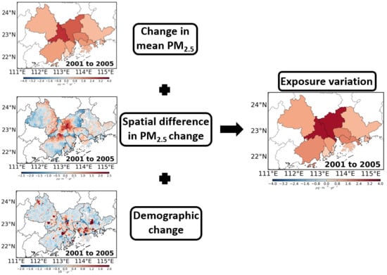
4.2. Decomposition of Exposure Variation

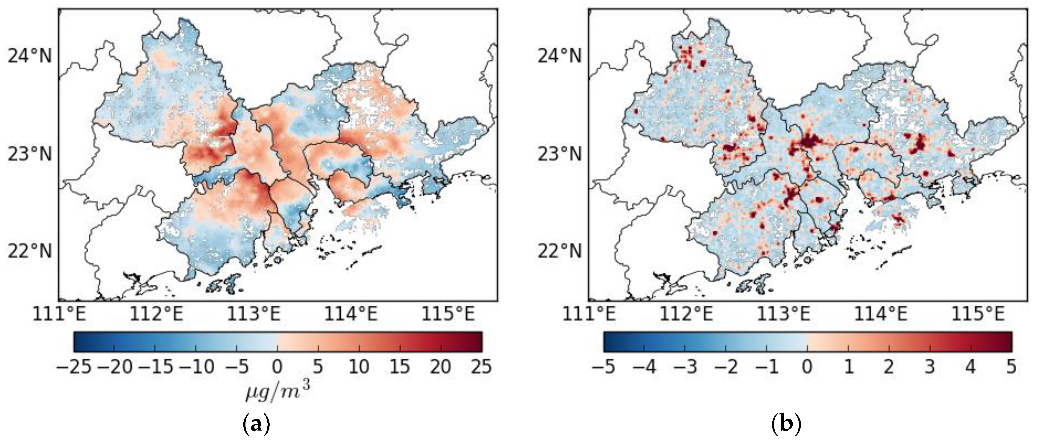
4.2.1. Effect of Changes in Mean PM2.5 Concentration

Figure 6 shows the trends in the population-weighted mean PM2.5 concentration resulting from changes in the mean PM2.5 concentration ( d c ρ 1 d t = d c 0 d t ) for different cities in the GBA region during the three most-recent FYP periods. During the 10th FYP period, all cities experienced an increase in c0. The most substantial increase in cρ resulting from increasing c0 was observed in Foshan, where the concentration increased by 2.77 µg/m3/year. During the 11th and 12th FYP periods, all cities experienced a decrease in c0. The most substantial reduction of cρ resulting from decreasing c0 was observed in Foshan, where the exposure level decreased by −2.25 µg/m3/year during the 11th FYP period and in Zhongshan, where the exposure level decreased by −3.71 µg/m3/year during the 12th FYP period.

4.2.2. The Effect of Spatial Differences in PM2.5 Change

Figure 7a shows the trends in the deviation of the PM2.5 concentration ( d C / d t ) for different cities during the three most-recent FYP periods. The areas with increasing c i , j values (in red) experienced less of a reduction of the PM2.5 concentration than those with decreasing c i , j values (in blue). During the 10th FYP period, densely populated urban areas ( p i , j > 0 ) experienced greater increases in the PM2.5 concentration than rural areas ( p i , j < 0 ) in most cities (8 out of 11). As a result, the spatial difference in the PM2.5 change increased cρ in these cities. The left panel of Figure 7b shows the trends in the population-weighted mean PM2.5 concentration resulting from the spatial difference in the PM2.5 change [ d c ρ 2 d t = 1 A · ( P · d C d t ) ] for different cities during the 10th FYP period. The most substantial increase in cρ resulting from the spatial difference in the PM2.5 change was observed in Guangzhou, where the exposure level increased by 1.03 µg/m3/year.
During the 11th and 12th FYP periods, densely populated urban areas ( p i , j > 0 ) experienced a greater decline in the PM2.5 concentration than rural areas ( p i , j < 0 ) in most cities (7 and 10 cities, respectively). As a result, the spatial difference in the PM2.5 change reduced cρ in these cities. The middle and right panels of Figure 7b show the trends in the population-weighted mean PM2.5 concentration resulting from the spatial difference in PM2.5 change for different cities during the 11th and 12th FYP periods, respectively. During the 11th FYP period, the effect reduced cρ most substantially in Guangzhou, where the exposure level decreased by −0.31 µg/m3/year. During the 12th FYP period, the effect reduced cρ most substantially in Macau, where the exposure level decreased by −0.58 µg/m3/year and in Shenzhen, where the exposure level decreased by −0.42 µg/m3/year.

4.2.3. The Effect of Demographic Change

Figure 8a plots trends in the relative deviation of population density ( d P / d t ) for different cities in the GBA region during the three most-recent FYP periods. The areas with increasing p i , j values (in red) experienced a greater percentage increase in the population density than those with decreasing p i , j values (in blue). It was found that urban areas in most cities experienced an increase in p i , j value. As these urban areas were typically more polluted than the rural areas, the increasing p i , j value in urban areas (typically with c i , j > 0 ) increased cρ in these cities. Figure 8b plots trends in the population-weighted mean PM2.5 concentration resulting from the demographic changes [ d c ρ 3 d t = 1 A · ( C · d P d t ) ] for different cities in the GBA region during the three most-recent FYP periods. The effect increased cρ by as much as 0.18 µg/m3/year.
Dongguan was a special case, in which the demographic change decreased cρ [i.e., 1 A · ( C · d P d t ) < 0 ] by as much as -0.10 µg/m3/year during the three FYP periods studied. Figure 9a shows the 15-year trend in the relative deviation of the population density ( d P / d t ) from 2001 to 2015 in Dongguan. It was found that the southeastern region experienced a greater increase of the population density than the northwestern region. To evaluate this demographic change, gross population data was collected for different towns in Dongguan from the statistical yearbook (http://tjj.dg.gov.cn). The ratios of the gross population for 2001 and 2015 in different towns are shown in Figure 10. The results showed that towns southeast of the city adjacent to Shenzhen experienced a greater percentage increase in population than those in the northwest. This population change characteristic is consistent with that using the gridded data.
Based on the 15-year average of PM2.5 concentration, Figure 9b shows the deviation of the PM2.5 concentration ( C ) in Dongguan. Higher PM2.5 concentrations were observed in the northwestern region, whereas lower PM2.5 concentrations were observed in the southeastern region. These results indicate that Dongguan rapidly developed residential areas in the cleaner regions that were adjacent to Shenzhen during the past decade. This demographic change pattern helped Dongguan reduce its population PM2.5 exposure level.

4.2.4. Long-Term Variation in PPCE

The variation in PPCE was determined by the combined effect of spatial differences in PM2.5 changes and demographic changes. Figure 11 shows the inter-annual variations in PPCE for different cities in the GBA region from 2001 to 2015. Most cities experienced an increase in PPCE during the 10th FYP period and a decrease in PPCE during the 12th FYP period. It is encouraging to find that the PPCE levels decreased to approximately half the previous maximum in most cities except in a few non-central cities such as Zhaoqing, Jiangmen and Huizhou. In 2015, the PPCE levels were still positive in all cities. The maximum PPCE levels in 2015 were found in Zhaoqing (3.7 µg/m3), Guangzhou (3.4 µg/m3) and Huizhou (3.2 µg/m3).

4.2.5. The Long-Term Variations in Population Exposure

The variations in the population-weighted mean PM2.5 concentration (cρ) were determined by the combined effect of changes in the mean PM2.5 concentration, spatial differences in PM2.5 change and demographic changes. Figure 12 shows inter-annual variations in cρ for different cities in the GBA region from 2001 to 2015. In general, the cρ values started to decrease during the 11th and 12th FYP periods in all cities. However, in 2015, the cρ values remained high in all cities. Although the lowest cρ value (cρ = 25.9 µg/m3 in Hong Kong) was lower than that of WHO IT-1, it still exceeded those of WHO IT-2, IT-3 and AQG.
Figure 13 shows the trends in the population-weighted mean PM2.5 concentration ( d c ρ / d t ) resulting from the combined effect for different cities in the GBA region during the three most-recent FYP periods. During the 10th FYP period, cρ increased in all cities. The most substantial increases in cρ were observed in Foshan, where the exposure level increased by 3.27 µg/m3/year and in Guangzhou, where the exposure level increased by 3.28 µg/m3/year. During the 11th and 12th FYP periods, cρ declined in all cities. The reduction in cρ was the most substantial in Foshan, where the exposure level decreased by −2.53 µg/m3/year during the 11th FYP period, and in Zhongshan, where the exposure level decreased by −3.78 µg/m3/year during the 12th FYP period.

5. Discussion

Lin et al. [17] compared the spatial mean and population-weighted mean PM2.5 concentrations for the cities in the GBA region from 2000 to 2014 and found that the population-weighted mean PM2.5 concentrations were systematically higher than the spatial averages. The systematic differences were related to the positive spatial correlation between the PM2.5 concentration and population density. For the entire GBA region, the population-weighted mean PM2.5 concentration was higher than the spatial average by 5.9 µg/m3. This study further investigated the characteristics of this difference using the pollution-population-coincidence induced PM2.5 exposure (PPCE). The PPCE is an important part of the population exposure level not only because its current level is significantly high, but also because its optimal level should be negative.
The mean PM2.5 concentration levels in all cities of the GBA region of China decreased during the 11th and 12th FYP periods, due to the implementation of improved control measures. In addition to the beneficial effect of the decreasing mean PM2.5 concentrations, it was found that spatial differences in the PM2.5 changes also reduced the population exposure levels in most cities during the 11th and 12th FYP periods. In contrast, demographic changes increased the exposure levels in most cities because of their rapid urbanization. Dongguan was a special case that experienced the best city planning in terms of reducing population exposure. The rapid development of residential areas in cleaner regions adjacent to Shenzhen reduced its population exposure level during the past decade.
Although the population exposure levels greatly decreased for cities in the GBA region during the past decade, their levels remained high because of the high mean PM2.5 concentrations and a positive PPCE. To better protect public health, more control efforts are required to reduce both the mean PM2.5 concentration and PPCE. Currently, the reduction of the mean PM2.5 concentration contributes significantly to the reduction of exposure levels in the GBA region. However, further reduction in the mean PM2.5 concentration becomes more difficult as it drops to a lower level. The positive PPCE levels in all cities suggest that unfavorable city planning has located residential dwellings in polluted areas. To reduce PPCE, it is suggested that control efforts further target densely populated areas (e.g., controls of mobile and residential sources) and that city planners relocate some sources of pollution (e.g., emissions from industrial sources or power generation) away from these densely populated urban areas and locate more residential dwellings in cleaner areas.
It is difficult to find a truly objective criterion to classify a geographical area as urban or rural. All classification methods require a choice of threshold, which is subjective to a certain extent. The Organization for Economic Co-operation and Development (OECD) uses population size cutoffs (50,000 or 100,000 people) and population density cutoffs (1000 or 1500 persons/km2 depending on the country) to define urban cores [33]. Following the OECD approach, Lin et al. [22] used the population density threshold of 1500 persons/km2 for the classification of urban and rural areas, and investigated the differences in PM2.5 variations between urban and rural areas for provinces in China. Their results showed that the urban areas in the GBA region experienced a greater increase in the PM2.5 concentration than did rural areas during the 10th FYP period and a greater decrease in PM2.5 concentration than did rural areas during the 11th and 12th FYP periods. These results are consistent with this study showing that the spatial difference in the PM2.5 change increased population exposure levels in most cities during the 10th FYP period and reduced population exposure levels in most cities during the 11th and 12th FYP periods.
The uncertainties of exposure assessment might result from both the PM2.5 concentration and population density. The evaluation of the satellite-derived PM2.5 concentration against ground observations in the GBA region obtained a correlation coefficient of 0.86 and a mean percentage bias of <20% [20]. To reduce the bias of the LandScan-derived population density data, the gridded population data was adjusted using gross population data collected from the statistical yearbooks. The assessment in this study focused on residential areas with population densities of ≥10 persons/km2. These residential areas contained 99.9% of the total population within the study region.
This study was focused on the decomposition of long-term variations in the population exposure to outdoor PM2.5, which were measured using a satellite remote sensing technique. The exposure to indoor PM2.5 would also negatively impact human health [34]. The indoor and outdoor exposure levels differ because of factors such as the spatial variability of the PM2.5 concentration and outdoor-to-indoor infiltration. The measurement of indoor pollution exposure requires advanced and portable sensor devices [35,36]. Future studies could assess the indoor exposure and its health impact using the sensor measurements.
The climate in the GBA region is affected by seasonal monsoons. The prevailing winds are from the north in winter and from the south in summer. The monsoons affect the monthly variation in the PM2.5 concentration in this region. Based on the satellite-derived monthly PM2.5 data, Figure 14 shows the monthly variation of the population-weighted mean PM2.5 concentration for different cities during the study period. All cities experienced lower population exposure levels in summer and higher population exposure levels in winter. The highest population exposure levels were typically found in January and December, with a level as high as >60 µg/m3 for cities in central GBA region (e.g., Foshan and Guangzhou). The population exposure levels actually doubled from summer to winter in several cities such as Zhongshan, Zhuhai and Jiangmen. Stronger regional transport of pollutants from inland, fewer mixing layers and less precipitation leads to higher levels of PM2.5 exposure in winter than in summer [17].
The highly developed economy and industry in the GBA region offer a large number of employment opportunities. Therefore, many residents in the GBA region come from other provinces and work in this region. During the Chinese New Year, which is usually a one-week holiday in February, most of these people move back to their hometowns. The movement of these people changes their short-term exposure levels. The changes are determined by the differences in the PM2.5 concentration level between the GBA region and their hometowns. Future studies could collect detailed information on the movement of populations over specific short-term periods and assess its effect on population exposure level.
The rapid economic development and urbanization in the GBA region has also caused complex environmental and health challenges from other air pollutants, such as sulfur dioxide (SO2), nitrate oxides (NOx) and ozone [37,38,39]. To better guide local environmental policies, it would be of great value to assess the population exposure to other air pollutants and the factors that influence such exposure. Further research could delineate exposure decompositions for other air pollutants in the study region.

6. Conclusions

This study used a decomposition method to assess the impact of PM2.5 variations and demographic changes on the exposure variations for cities in the GBA region of China during the three most-recent FYP periods. This study took advantage of high-resolution satellite observations to characterize the long-term variation in human exposure to PM2.5. The results showed that the 15-year average PPCE levels were positive in all cities, suggesting that unfavorable city planning had placed people in the polluted areas. The analyses of the spatial differences in PM2.5 changes showed that urban areas experienced a greater decrease in the PM2.5 concentration than rural areas did in most cities during the 11th (2006–2010) and 12th (2011–2015) FYP periods. These spatial differences in PM2.5 changes reduced their PPCE levels and thus reduced the exposure levels. The migration of population resulting from rapid urbanization, however, increased the PPCE and exposure levels in most cities during the three FYP periods considered. Dongguan was the only city in which the demographic change reduced the exposure level because of its rapid development of residential areas in cleaner regions adjacent to Shenzhen. The exposure levels in all cities remained high because of the high mean PM2.5 concentrations and their positive PPCE. To better protect public health, control efforts should target densely populated areas and city planning should place more residential dwellings in cleaner areas.

Author Contributions

The composition of the manuscript was supervised by A.K.H.L.; C.L. (Changqing Lin) drafted the original manuscript; J.C.H.F., Q.H., J.M., X.L., Z.L., C.L. (Chengcai Li), R.Z. and A.H.S.W. edited the manuscript.

Funding

This work was supported by the Research Grants Council of Hong Kong Government (Project No. T24/504/17), the Science and Technology Plan Project of Guangdong Province of China (Grant No. 2017A050506003), NSFC/RGC (Grant N_HKUST631/05), and the Fok Ying Tung Graduate School (NRC06/07.SC01).

Acknowledgments

We thank the Hong Kong Environmental Protection Department for provision of air-quality monitoring data.

Conflicts of Interest

The authors declare no conflicts of interest. The funders had no role in the design of the study; in the collection, analyses, or interpretation of data; in the writing of the manuscript; or in the decision to publish the results.

Abbreviations

GBAGreater Bay Area
PRDPearl River Delta
FYPFive-Year Plan
AODAerosol optical depth
PM2.5Fine particulate matter
MODISModerate Resolution Imaging Spectroradiometer
WHOWorld Health Organization
IT-1Interim Target 1
IT-2Interim Target 2
IT-3Interim Target 3
AQGAir Quality Guideline
NAAQSChinese National Ambient Air Quality Standard
GZGuangzhou city
SZShenzhen city
ZHZhuhai city
DGDongguan city
FSFoshan city
ZSZhongshan city
ZQZhaoqing city
JMJiangmen city
HZHuizhou city
HKHong Kong special administrative zone
MCMacau special administrative zone
cρPopulation-weighted mean PM2.5 concentration
c i , j Spatial distribution of PM2.5 concentration
ρ i , j Spatial distribution of population density
c0Spatial average of PM2.5 concentration
ρ0Spatial average of population density
AArea of the study region
c i , j Deviation of PM2.5 concentration from c0
ρ i , j Deviation of population density from ρ0
p i , j Relative deviation of population density from ρ0
C Matrix of c i , j
P Matrix of p i , j
PPCE (c1)Pollution-population-coincidence–induced PM2.5 exposure

Appendix: Exposure decomposition

In a two-dimensional region, the spatial distribution of PM2.5 concentration is denoted as c i , j and population density is denoted as ρ i , j , where i = {1, 2, 3,…, X} and j = {1, 2, 3,…, Y}. This study used c0 and ρ0 to represent the spatial averages of the PM2.5 concentration and population density, respectively, in the study region. They can be respectively expressed as Equations (A1.1) and (A1.2):
c 0 = 1 A i = 1 X j = 1 Y c i , j
ρ 0 = 1 A i = 1 X j = 1 Y ρ i , j
where A = X·Y is the total grid number, representing the area of the study region. Then, c i , j and ρ i , j are defined as the deviation of the PM2.5 concentration from c0 and the deviation of population density from ρ0, respectively. They can be respectively expressed as Equations (A2.1) and (A2.2)
c i , j = c i , j c 0
ρ i , j = ρ i , j ρ 0
The c i , j values are positive in polluted areas and negative in clean areas. The ρ i , j values are positive in densely populated urban areas and negative in rural areas. By definition, Equations (A3.1) and (A3.2) are as follows:
i = 1 X j = 1 Y c i , j = 0
i = 1 X j = 1 Y ρ i , j = 0
The population-weighted mean PM2.5 concentration (cρ) can be quantified by Equation (A4):
c ρ = i = 1 X j = 1 Y c i , j · ρ i , j i = 1 X j = 1 Y ρ i , j
Or, it can be expressed as Equations (A5.1) and (A5.2):
c ρ = i = 1 X j = 1 Y ( c 0 + c i , j ) · ( ρ 0 + ρ i , j ) ρ 0 · A
c ρ = i = 1 X j = 1 Y ( c 0 · ρ 0 + c 0 · ρ i , j + c i , j · ρ 0 + c i , j · ρ i , j ) ρ 0 · A
By separating out c0, cρ can be expressed as Equations (A6.1) and (A6.2):
c ρ = c 0 + i = 1 X j = 1 Y c i , j · ρ i , j ρ 0 · A
c ρ = c 0 + 1 A · i = 1 X j = 1 Y ( c i , j c 0 ) · ( ρ i , j ρ 0 ) ρ 0
Equation(A7) can be defined as:
p i , j = ρ i , j ρ 0 ρ 0
to represent the normalized deviation of the population density from ρ0. cρ can then be expressed as Equation (A8):
c ρ = c 0 + 1 A · i = 1 X j = 1 Y c i , j · p i , j
Furthermore, C and P are defined as Matrices of c i , j and p i , j , respectively. Then, cρ can be expressed as Equation (A9):
c ρ = c 0 + 1 A · ( C · P )
The cρ value is therefore determined by the mean PM2.5 concentration (c0) together with a dot product of the deviation of the PM2.5 concentration ( C ) and the normalized deviation of the population density ( P ). The second part of cρ is associated with the spatial coincidence between the population density and PM2.5 concentration. A pollution-population-coincidence–induced PM2.5 exposure (PPCE) of c1 was used to represent the PM2.5 exposure resulting from this effect. This PPCE (c1) can be expressed as Equation (A10):
c 1 = 1 A · ( C · P )
cρ can then be expressed as Equation (A11):
c ρ = c 0 + c 1
The cρ value can be decomposed into two parts. The first part is the mean PM2.5 concentration (c0) and the second part is PPCE (c1). An increase in population density in polluted areas leads to a positive value of c1, which boosts the cρ level. To lessen the human exposure to PM2.5, the most successful control strategies must simultaneously decrease the mean PM2.5 concentration (c0) and the PPCE (c1). The trend in cρ can be expressed as Equation (A12):
d c ρ d t = d c 0 d t + d c 1 d t
The trend in c1 can be expressed as Equation (A13):
d c 1 d t = 1 A · ( P · d C d t ) + 1 A · ( C · d P d t )
The elements of the trends in C and P can be expressed as Equations (A14.1) and (A14.2):
d c i , j d t = d ( c i , j c 0 ) d t = d c i , j d t d c 0 d t
d p i , j d t = d ( ρ i , j ρ 0 ρ 0 ) d t = ρ i , j ρ 0 ( 1 ρ i , j d ρ i , j d t 1 ρ 0 d ρ 0 d t )
The c i , j values decline in areas where the PM2.5 concentrations undergo a greater reduction than the average level. The p i , j values decline in areas where the population densities undergo a greater percentage reduction than the average level. When ρ0 is relatively stable (i.e., d ρ 0 d t 0 ), the p i , j values decrease in areas where population densities decrease (i.e., people migrate out of the area). In contrast, the p i , j values increase in areas where population densities increase (i.e., people migrate into the areas).
The trend in cρ can then be expressed as Equation (A15):
d c ρ d t = d c 0 d t + 1 A · ( P · d C d t ) + 1 A · ( C · d P d t )
The trend in cρ can be decomposed into three parts (Equations (A16.1–16.3)):
d c ρ 1 d t = d c 0 d t
d c ρ 2 d t = 1 A · ( P · d C d t )
d c ρ 3 d t = 1 A · ( C · d P d t )
The cρ value therefore decreases under three conditions: (a)   d c 0 d t < 0 ; (b) P · d C d t < 0 ; or (c) C · d P d t < 0 . The first condition can be achieved if the mean PM2.5 concentration decreases. The second condition occurs when d c i , j d t < 0 in populous urban areas with p i , j > 0 , whereas d c i , j d t > 0 in rural areas with p i , j < 0 . This condition can be achieved if the PM2.5 concentration within populous urban areas reduces more than it does within rural areas. The third condition takes place when d p i , j d t < 0 in polluted areas with c i , j > 0 , whereas d p i , j d t > 0 in clean areas with c i , j < 0 . This condition can be achieved if city planning relocates people from living in polluted areas to clean areas. In summary, the variation in cρ can be decomposed into three parts, which are associated with the change in the mean PM2.5 concentration, the spatial difference in PM2.5 change and the demographic change, respectively.

References

  1. Bo, Y.; Guo, C.; Lin, C.; Chang, L.; Chan, T.C.; Huang, B.; Lee, K.P.; Tam, T.; Lau, A.K.H.; Lao, X.Q.; et al. Dynamic Changes in Long-Term Exposure to Ambient Particulate Matter and Incidence of Hypertension in Adults. Hypertension 2019, 74, 669–677. [Google Scholar] [CrossRef] [PubMed]
  2. Chan, T.C.; Zhang, Z.; Lin, B.C.; Lin, C.; Deng, H.B.; Chuang, Y.C.; Chan, J.W.M.; Jiang, W.K.; Tam, T.; Chang, L.; et al. Long-Term Exposure to Ambient Fine Particulate Matter and Chronic Kidney Disease: A Cohort Study. Environ. Health Perspect. 2018, 126, 107002. [Google Scholar] [CrossRef] [PubMed]
  3. Guo, C.; Zhang, Z.; Lau, A.K.H.; Lin, C.Q.; Chuang, Y.C.; Chan, J.; Jiang, W.K.; Tam, T.; Yeoh, E.K.; Chan, T.C.; et al. Effect of long-term exposure to fine particulate matter on lung function decline and risk of chronic obstructive pulmonary disease in Taiwan: A longitudinal, cohort study. Lancet Planet. Health 2018, 2, e114–e125. [Google Scholar] [CrossRef]
  4. Lao, X.Q.; Guo, C.; Chang, L.; Bo, Y.; Zhang, Z.; Chuang, Y.C.; Jiang, W.K.; Lin, C.; Tam, T.; Lau, A.K.H.; et al. Long-term exposure to ambient fine particulate matter (PM2.5) and incident type 2 diabetes: A longitudinal cohort study. Diabetologia 2019, 62, 759–769. [Google Scholar] [CrossRef] [PubMed]
  5. Zhang, Z.; Chan, T.C.; Guo, C.; Chang, L.; Lin, C.; Chuang, Y.C.; Jiang, W.K.; Ho, K.F.; Tam, T.; Woo, K.S.; et al. Long-term exposure to ambient particulate matter (PM2.5) is associated with platelet counts in adults. Environ. Pollut. 2018, 240, 432–439. [Google Scholar] [CrossRef] [PubMed]
  6. Apte, J.S.; Marshall, J.D.; Cohen, A.J.; Brauer, M. Addressing Global Mortality from Ambient PM2.5. Environ. Sci. Technol. 2015, 49, 8057–8066. [Google Scholar] [CrossRef] [PubMed]
  7. Zhong, L.; Louie, P.K.K.; Zheng, J.; Yuan, Z.; Yue, D.; Ho, J.W.K.; Lau, A.K.H. Science–policy interplay: Air quality management in the Pearl River Delta region and Hong Kong. Atmos. Environ. 2013, 76, 3–10. [Google Scholar] [CrossRef]
  8. Aunan, K.; Ma, Q.; Lund, M.T.; Wang, S. Population-weighted exposure to PM2.5 pollution in China: An integrated approach. Environ. Int. 2018, 120, 111–120. [Google Scholar] [CrossRef]
  9. Brauer, M.; Amann, M.; Burnett, R.T.; Cohen, A.; Dentener, F.; Ezzati, M.; Henderson, S.B.; Krzyzanowski, M.; Martin, R.V.; Van Dingenen, R.; et al. Exposure Assessment for Estimation of the Global Burden of Disease Attributable to Outdoor Air Pollution. Environ. Sci. Technol. 2012, 46, 652–660. [Google Scholar] [CrossRef]
  10. David, L.M.; Ravishankara, A.R.; Kodros, J.K.; Pierce, J.R.; Venkataraman, C.; Sadavarte, P. Premature Mortality Due to PM2.5 Over India: Effect of Atmospheric Transport and Anthropogenic Emissions. GeoHealth 2019, 3, 2–10. [Google Scholar] [CrossRef]
  11. Van Donkelaar, A.; Martin, R.V.; Brauer, M.; Boys, B.L. Use of satellite observations for long-term exposure assessment of global concentrations of fine particulate matter. Environ. Health Perspect. 2015, 123, 135–143. [Google Scholar] [CrossRef] [PubMed]
  12. Gui, K.; Che, H.; Wang, Y.; Wang, H.; Zhang, L.; Zhao, H.; Zheng, Y.; Sun, T.; Zhang, X. Satellite-derived PM2.5 concentration trends over Eastern China from 1998 to 2016: Relationships to emissions and meteorological parameters. Environ. Pollut. 2019, 247, 1125–1133. [Google Scholar] [CrossRef] [PubMed]
  13. Li, J.; Zhu, Y.; Kelly, J.T.; Jang, C.J.; Wang, S.; Hanna, A.; Xing, J.; Lin, C.J.; Long, S.; Yu, L. Health benefit assessment of PM2.5 reduction in Pearl River Delta region of China using a model-monitor data fusion approach. J. Environ. Manag. 2019, 233, 489–498. [Google Scholar] [CrossRef] [PubMed]
  14. Xue, T.; Zheng, Y.; Tong, D.; Zheng, B.; Li, X.; Zhu, T.; Zhang, Q. Spatiotemporal continuous estimates of PM2.5 concentrations in China, 2000–2016: A machine learning method with inputs from satellites, chemical transport model, and ground observations. Environ. Int. 2019, 123, 345–357. [Google Scholar] [CrossRef]
  15. Zheng, H.; Zhao, B.; Wang, S.; Wang, T.; Ding, D.; Chang, X.; Liu, K.; Xing, J.; Dong, Z.; Aunan, K.; et al. Transition in source contributions of PM2.5 exposure and associated premature mortality in China during 2005–2015. Environ. Int. 2019, 132, 105111. [Google Scholar] [CrossRef]
  16. Burnett, R.; Chen, H.; Szyszkowicz, M.; Fann, N.; Hubbell, B.; Pope, C.A.; Apte, J.S.; Brauer, M.; Cohen, A.; Weichenthal, S.; et al. Global estimates of mortality associated with long-term exposure to outdoor fine particulate matter. Proc. Natl. Acad. Sci. USA 2018, 115, 9592–9597. [Google Scholar] [CrossRef]
  17. Lin, C.Q.; Li, Y.; Lau, A.K.H.; Deng, X.J.; Tse, K.T.; Fung, J.C.H.; Li, C.C.; Li, Z.Y.; Lu, X.C.; Zhang, X.G.; et al. Estimation of long-term population exposure to PM2.5 for dense urban areas using 1-km MODIS data. Remote Sens. Environ. 2016, 179, 13–22. [Google Scholar] [CrossRef]
  18. Lu, Q.; Zheng, J.; Ye, S.; Shen, X.; Yuan, Z.; Yin, S. Emission trends and source characteristics of SO2, NOx, PM10 and VOCs in the Pearl River Delta region from 2000 to 2009. Atmos. Environ. 2013, 76, 11–20. [Google Scholar] [CrossRef]
  19. Ma, Z.; Hu, X.; Sayer, A.M.; Levy, R.; Zhang, Q.; Xue, Y.; Tong, S.; Bi, J.; Huang, L.; Liu, Y. Satellite-Based Spatiotemporal Trends in PM2.5 Concentrations: China, 2004–2013. Environ. Health Perspect. 2016, 124, 184–192. [Google Scholar] [CrossRef]
  20. Lin, C.Q.; Li, Y.; Lau, A.K.H.; Li, C.C.; Fung, J.C.H. 15-Year PM2.5 Trends in the Pearl River Delta Region and Hong Kong from Satellite Observation. Aerosol Air Qual. Res. 2018, 18, 2355–2362. [Google Scholar] [CrossRef]
  21. Lin, C.; Lau, A.K.H.; Lu, X.; Fung, J.C.H.; Li, Z.; Li, C.; Wong, A.H.S. Assessing Effect of Targeting Reduction of PM2.5 Concentration on Human Exposure and Health Burden in Hong Kong Using Satellite Observation. Remote Sens. 2018, 10, 2064. [Google Scholar] [CrossRef]
  22. Lin, C.Q.; Lau, A.K.H.; Li, Y.; Fung, J.C.H.; Li, C.C.; Lu, X.C.; Li, Z.Y. Difference in PM2.5 variations between urban and rural areas over eastern China from 2001 to 2015. Atmosphere 2018, 9, 312. [Google Scholar] [CrossRef]
  23. Wang, J.; Zhao, B.; Wang, S.; Yang, F.; Xing, J.; Morawska, L.; Ding, A.; Kulmala, M.; Kerminen, V.M.; Kujansuu, J.; et al. Particulate matter pollution over China and the effects of control policies. Sci. Total Environ. 2017, 584–585, 426–447. [Google Scholar] [CrossRef]
  24. Lin, C.; Lau, A.K.H.; Fung, J.C.H.; Lao, X.Q.; Li, Y.; Li, C. Assessing the Effect of the Long-Term Variations in Aerosol Characteristics on Satellite Remote Sensing of PM2.5 Using an Observation-Based Model. Environ. Sci. Technol. 2019, 53, 2990–3000. [Google Scholar] [CrossRef] [PubMed]
  25. Lin, C.Q.; Li, C.C.; Lau, A.K.H.; Yuan, Z.B.; Lu, X.C.; Tse, K.T.; Fung, J.C.H.; Li, Y.; Yao, T.; Su, L.; et al. Assessment of satellite-based aerosol optical depth using continuous lidar observation. Atmos. Environ. 2016, 140, 273–282. [Google Scholar] [CrossRef]
  26. Li, Y.; Lin, C.; Lau, A.K.H.; Liao, C.; Zhang, Y.; Zeng, W.; Li, C.; Fung, J.C.H.; Tse, T.K.T. Assessing Long-Term Trend of Particulate Matter Pollution in the Pearl River Delta Region Using Satellite Remote Sensing. Environ. Sci. Technol. 2015, 49, 11670–11678. [Google Scholar] [CrossRef]
  27. Li, C.; Lau, A.K.H.; Mao, J.; Chu, D.A. Retrieval, validation, and application of the 1-km aerosol optical depth from MODIS measurements over Hong Kong. IEEE Trans. Geosci. Remote Sens. 2005, 43, 2650–2658. [Google Scholar]
  28. Lin, C.Q.; Li, Y.; Yuan, Z.B.; Lau, A.K.H.; Li, C.C.; Fung, J.C.H. Using satellite remote sensing data to estimate the high-resolution distribution of ground-level PM2.5. Remote Sens. Environ. 2015, 156, 117–128. [Google Scholar] [CrossRef]
  29. Lin, C.Q.; Liu, G.; Lau, A.K.H.; Li, Y.; Li, C.C.; Fung, J.C.H.; Lao, X.Q. High-resolution satellite remote sensing of provincial PM2.5 trends in China from 2001 to 2015. Atmos. Environ. 2018, 180, 110–116. [Google Scholar] [CrossRef]
  30. Geng, G.; Zhang, Q.; Martin, R.V.; van Donkelaar, A.; Huo, H.; Che, H.; Lin, J.; He, K. Estimating long-term PM2.5 concentrations in China using satellite-based aerosol optical depth and a chemical transport model. Remote Sens. Environ. 2015, 166, 262–270. [Google Scholar] [CrossRef]
  31. Peng, J.; Chen, S.; Lü, H.; Liu, Y.; Wu, J. Spatiotemporal patterns of remotely sensed PM2.5 concentration in China from 1999 to 2011. Remote Sens. Environ. 2016, 174, 109–121. [Google Scholar] [CrossRef]
  32. Van Donkelaar, A.; Martin, R.V.; Brauer, M.; Kahn, R.; Levy, R.; Verduzco, C.; Villeneuve, P.J. Global estimates of ambient fine particulate matter concentrations from satellite-based aerosol optical depth: Development and application. Environ. Health Perspect. 2010, 118, 847–855. [Google Scholar] [CrossRef] [PubMed] [Green Version]
  33. OECD. Redefining “Urban”: A New Way to Measure Metropolitan Areas; OECD Publishing: Paris, France, 2012. [Google Scholar]
  34. Li, Z.; Wen, Q.; Zhang, R. Sources, health effects and control strategies of indoor fine particulate matter (PM2.5): A review. Sci. Total Environ. 2017, 586, 610–622. [Google Scholar] [CrossRef] [PubMed]
  35. Li, Z.; Che, W.; Lau, A.K.H.; Fung, J.C.H.; Lin, C.; Lu, X. A feasible experimental framework for field calibration of portable light-scattering aerosol monitors: Case of TSI DustTrak. Environ. Pollut. 2019, 255, 113136. [Google Scholar] [CrossRef] [PubMed]
  36. Li, Z.; Che, W.; Frey, H.C.; Lau, A.K.H.; Lin, C. Characterization of PM2.5 exposure concentration in transport microenvironments using portable monitors. Environ. Pollut. 2017, 228, 433–442. [Google Scholar] [CrossRef]
  37. Li, Y.; Lau, A.K.H.; Fung, J.C.H.; Ma, H.; Tse, Y. Systematic evaluation of ozone control policies using an Ozone Source Apportionment method. Atmos. Environ. 2013, 76, 136–146. [Google Scholar] [CrossRef]
  38. Lu, X.; Yao, T.; Li, Y.; Fung, J.C.H.; Lau, A.K.H. Source apportionment and health effect of NOx over the Pearl River Delta region in southern China. Environ. Pollut. 2016, 212, 135–146. [Google Scholar] [CrossRef] [Green Version]
  39. Wang, X.; Liu, H.; Pang, J.; Carmichael, G.; He, K.; Fan, Q.; Zhong, L.; Wu, Z.; Zhang, J. Reductions in sulfur pollution in the Pearl River Delta region, China: Assessing the effectiveness of emission controls. Atmos. Environ. 2013, 76, 113–124. [Google Scholar] [CrossRef]
Figure 1. The spatial distribution of the 15-year mean of the population density at a spatial resolution of 0.01° × 0.01° in the Greater Bay Area (GBA) region of China.
Remotesensing 11 02646 g001
Figure 2. The spatial distribution of the 15-year mean of PM2.5 concentration at a spatial resolution of 0.01° × 0.01° in the residential areas of the GBA region.
Remotesensing 11 02646 g002
Figure 3. The 15-year averages of (a) the deviation of PM2.5 concentration ( C ) and (b) the normalized deviation of population density ( P ) for different cities in the GBA region.
Remotesensing 11 02646 g003
Figure 4. The 15-year average of pollution-population-coincidence–induced PM2.5 exposure (PPCE) (c1) for different cities in the GBA region.
Remotesensing 11 02646 g004
Figure 5. The 15-year averages of the mean PM2.5 concentration (c0, blue bars) and the population-weighted mean PM2.5 concentration (cρ, red bars) for different cities in the GBA region. The cities are ordered according to their c0 values.
Remotesensing 11 02646 g005
Figure 6. Trends in the population-weighted mean PM2.5 concentration resulting from changes in the mean PM2.5 concentration ( d c ρ 1 d t = d c 0 d t ) for different cities in the GBA region during the three most-recent Five-Year Plan (FYP) periods.
Remotesensing 11 02646 g006
Figure 7. (a) Trends in the deviation of the PM2.5 concentration ( d C / d t ) for different cities during the three most-recent FYP periods. (b) Trends in the population-weighted mean PM2.5 concentration resulting from the spatial differences in PM2.5 changes [ d c ρ 2 d t = 1 A · ( P · d C d t ) ] for different cities during the three most-recent FYP periods.
Remotesensing 11 02646 g007
Figure 8. (a) Trends in the relative deviation of the population density ( d P / d t ) for different cities in the GBA region during the three most-recent FYP periods. (b) Trends in the population-weighted mean PM2.5 concentration resulting from demographic changes [ d c ρ 3 d t = 1 A · ( C · d P d t ) ] for different cities in the GBA region during the three most-recent FYP periods.
Remotesensing 11 02646 g008
Figure 9. (a) The trend in the relative deviation of the population density ( d P / d t ) from 2001 to 2015 in Dongguan. (b) The 15-year average of the deviation of the PM2.5 concentration ( C ) in Dongguan.
Remotesensing 11 02646 g009
Figure 10. The ratios of gross population for 2001 and 2015 for different towns in Dongguan. The numbers in red indicate towns with ratios that were higher than the city average. In contrast, the numbers in blue indicate towns with ratios that were lower than the city average.
Remotesensing 11 02646 g010
Figure 11. Inter-annual variations in the PPCE for different cities in the GBA region from 2001 to 2015.
Remotesensing 11 02646 g011
Figure 12. The inter-annual variations in the population-weighted mean PM2.5 concentration (cρ) for different cities in the GBA region from 2001 to 2015.
Remotesensing 11 02646 g012
Figure 13. The trends in the population-weighted mean PM2.5 concentration ( d c ρ / d t ) for different cities in the GBA region during the three FYP periods.
Remotesensing 11 02646 g013
Figure 14. The monthly variation in the population-weighted mean PM2.5 concentration (cρ) for different cities in the GBA region during the entire study period.
Remotesensing 11 02646 g014

