Sensitivity of Radar Altimeter Waveform to Changes in Sea Ice Type at Resolution of Synthetic Aperture Radar

Abstract

Radar altimetry in the context of sea ice has mostly been exploited to retrieve basin-scale information about sea ice thickness. In this paper, we investigate the sensitivity of altimetric waveforms to small-scale changes (a few hundred meters to about 10 km) of the sea ice surface. Near-coincidental synthetic aperture radar (SAR) imagery and CryoSat-2 altimetric data in the Beaufort Sea are used to identify and study the spatial evolution of altimeter waveforms over these features. Open water and thin ice features are easily identified because of their high peak power waveforms. Thicker ice features such as ridges and multiyear ice floes of a few hundred meters cause a response in the waveform. However, these changes are not reflected in freeboard estimates. Retrieval of robust freeboard estimates requires homogeneous floes in the order of 10 km along-track and a few kilometers to both sides across-track. We conclude that the combination of SAR imagery and altimeter data could improve the local sea ice picture by extending spatially scarce freeboard estimates to regions of similar SAR signature.

1. Introduction

Active radar remote sensing plays a key role for high-resolution observations of the Arctic sea ice cover in the order of a hundred meters to a kilometer. Synthetic aperture radar (SAR) imagery carries information, for example, about sea ice concentration and extent, sea ice types and sea ice drift, e.g., [1]. Radar altimetry is the primary tool to estimate sea ice thickness with good accuracy on basin-scale [2,3]. The altimeter measures the sea ice freeboard, i.e., the distance between the ocean and the sea ice surface, and ice thickness can then be calculated assuming hydrostatic equilibrium and auxiliary information about sea ice density, i.e., sea ice type, and snow load [4]. To reduce the dependence on auxiliary information, the direct retrieval of sea ice type from altimeter waveform data has been investigated and showed promising results, but also a large variability of waveform parameters [5,6,7,8]. The introduction of the delay/Doppler or SAR altimeter has significantly increased the along-track resolution of spaceborne altimetric measurements [9,10]. This results in better sensitivity to small features on the surface [11] and enables the ability to investigate the response of altimeter waveforms to small-scale variations of sea ice types such as large ridges, refrozen leads or multiyear sea ice floes embedded in first-year sea ice on spatial scales from a few hundred meters to a few tens of kilometers.

Altimetric data alone is, however, not sufficient to unambiguously determine the origin of waveform changes over sea ice, because of temporal and spatial variability of waveforms and the impact of off-nadir specular reflectors [6,7,12]. Near-coincidental SAR imagery has proven a valuable source for verification of lead detection algorithms in altimeter data processing, e.g., [13,14]. In the late 1980s, two studies have been undertaken with data from Seasat and Geosat to relate SAR backscatter and altimetric data over sea ice, but both were limited to one SAR image as a reference [15,16]. Presently however, Copernicus’ Sentinel-1 and Sentinel-3 two satellite constellations in addition to Radarsat-2/Radarsat-Constellation and CryoSat-2 provide an increasing and long term (Copernicus program) data availability especially at lower latitudes (below 81.5${}^{\circ }$). Furthermore, near real time availability of data [17] facilitates the use for short term observations of the sea ice cover. This allows us to perform, to the best of our knowledge, the first comprehensive study of the waveform evolution over different sea ice types with SAR imagery as high-resolution validation data.

SAR imagery gives a high-resolution, two-dimensional picture of the current sea ice situation, but sea ice thickness can only be inferred from sea ice signatures with ambiguities [18]. Meanwhile, altimeter data provides a means to obtain sea ice thickness, but is sparse in nature due to the one-dimensionality of the measurements. To overcome these spatial limitations, averaging in space and time is commonly applied to obtain standard products of hemispherical sea ice freeboard and thickness, e.g., [19], at the expense of small-scale features. Combining these two information sources therefore has several potential benefits. On the one hand, sea ice type information, necessary for freeboard to thickness conversion [4], can be provided by SAR imagery in high-resolution [20] to reduce uncertainties in this critical step. On the other hand, the scarce thickness retrievals could be locally expanded to neighboring areas with similar sea ice signature in the SAR image regarding backscatter intensity and texture.

In this paper, we use near-coincidental Sentinel-1 SAR imagery and CryoSat-2 altimeter data of three winter seasons in the Beaufort Sea to investigate the sensitivity of altimeter waveforms to small-scale (up to 10–20 km) variations of sea ice. We evaluate whether SAR imagery aids the interpretation of the sea ice situation and identification of sea ice types. Furthermore, we derive dimensions of such features to obtain meaningful freeboard estimates. The study area and data are presented in Section 2. The backscatter and altimeter parameters are presented in Section 3 and analyzed in Section 4, focusing first on the distinct waveform properties of the different ice types (4.1) and then on local features (4.2). We conclude with a discussion on how SAR imagery and altimetry can be used to augment each other’s ability for sea ice monitoring.

2. Data

Figure 1 shows the study area within the Beaufort Sea, located in the Arctic. Blue areas represent the Sentinel-1 images and the red lines the CryoSat-2 altimeter ground tracks. The Beaufort Sea was chosen for this study because first-year and multiyear sea ice are present during wintertime in this area. Furthermore, a belt of larger multiyear ice floes embedded in first-year ice can usually be found in this area and is thus ideal for studying the ability to detect small-scale changes in sea ice. We collected near-coincidental Sentinel-1 SAR imagery and CryoSat-2 altimeter data of three winter seasons (Feb/Mar 2016, Nov/Dec/Jan 2016/17 and Jan/Feb/Mar 2018) with an average time lag from 34 min ranging from a few to about 80 min. For drift speeds up to about 6 cm/s the motion will be below the along-track resolution of the altimeter (about 300 m) for all time lags. Higher drift speeds are possible in this area [21] and therefore sea ice drift can exceed the altimeter footprint size for larger time lags.

2.1. Sentinel-1 A/B

We used 73 Copernicus Sentinel-1 A/B dual-polarization C-band (5.405 GHz $\widehat{=}$ 5.6 cm) SAR images taken between February 2016 and March 2018.

Table 1. Overview of Sentinel-1 data and time lags with respect to CryoSat acquisitions.

Date	Number of Images	Number of Sequences	Mean Time Lag [min]	Min/Max Time Lag [min]
Feb 2016	3	1	61	-
Mar 2016	12	6	27	3/54
Nov 2016	6	3	46	28/69
Dec 2016	9	4	27	2/40
Jan 2017	5	2	44	27/61
Jan 2018	4	2	55	53/56
Feb 2018	28	14	33	4/74
Mar 2018	6	4	44	26/75
Total	73	36

summarizes the temporal distribution of the data where a sequence denotes up to three sequential images connected to the same near-coincidental altimeter track. All images are extra wide swath ground range detected with medium resolution, i.e., 40 m × 40 m pixel size and range and azimuth resolution of 93 m and 87 m, respectively. The polarization is horizontal transmit and receive (co-polarization, HH) and horizontal transmit and vertical receive (cross-polarization, HV). The data is preprocessed using the Sentinel Application Toolbox (SNAP) applying the following steps: precise orbit → noise removal → (optional) slice assembly → calibration to ${\sigma }^0$→ terrain correction to UTM with ASTER 1 sec GDEM.

2.2. CryoSat-2

We used 35 CryoSat-2 altimeter tracks that were near-coinciding with the Sentinel-1 images to analyze waveform response and behavior for different ice types and small-scale features. The SIRAL altimeter aboard CryoSat-2 is a K_u-band (13.575 GHz $\widehat{=}$ 2.2 cm) altimeter that operates in SAR (delay/Doppler) mode over sea ice. Sequences of radar bursts are emitted by the radar forming a stack of waveforms that view the same area on the ground from different viewing angles. The range corrected waveforms are averaged, and these multi-looked waveforms are provided alongside so-called stack parameters that describe the angular behavior of delay time integrated power [10]. The pulse limited footprint size in SAR mode is approximately 300 m along-track and 1.5 km across-track [22]. The distance between range bins of the multi-looked waveforms is 23.42 cm and a full waveform of 256 bins covers a range window of 60 m, whereas the range resolution is about 47 cm [23]. The high orbital inclination of the satellite (92 ${}^{\circ }$) allows observations up to 88 ${}^{\circ }$ N in the Arctic. CryoSat data provided by ESA is used in this study. Waveform parameters are obtained from level 1b Baseline C data and freeboard measurements are taken from level 2 data. For the analysis in this study no further processing of the data is performed.

3. Methods

3.1. SAR Image and Waveform Parameters

Comparison of SAR imagery and altimeter waveform data requires the spatial overlap of both data sets. Consecutive SAR images of the same orbit were assembled into one single image and corresponding altimeter tracks located using the geolocation information of the product. Rectangular polygons with a length of 300 m in along-track and 1.5 km in across-track direction were calculated around each altimeter track point. This size resembles the footprint size of the altimeter associated with the first peak of the return [22]. The mean value of backscatter intensity ${\sigma }^0$ at co- and cross-polarization of this polygon is calculated for comparison with parameters describing the shape of the altimeter waveform.

SAR instruments and altimeters perceive sea ice surface information differently because of their viewing geometry, e.g., side-looking for SAR imagery and nadir-looking for distance measuring altimeters [24,25]. Smooth surfaces, i.e., flat open water or thin ice, have a low backscatter intensity in SAR imagery while altimeter waveforms show a narrow peak with high power. With increasing roughness of the surface, SAR backscatter intensities increase, and altimeter waveforms become more diffuse with lower peak power and larger power values in the tail of the waveform. Figure 2 shows examples of typical waveforms for leads, first-year and multiyear sea ice. Note the differences of the scaling of the y-axis.

In this study, we used pulse peakiness (PP), scaled inverse mean power (IMP) and stack standard deviation (SSD) as parameters to characterize the shape of the waveform. The first two are derived from the waveform while SSD is a stack parameter that is provided as auxiliary information with the data set. The maximum peak power is a helpful parameter for visual waveform interpretation but contains similar information as PP. PP is used in the quantitative analysis whereas peak power is used for qualitative description of spatial waveform evolution.

PP is a measure for how much power is contained in the maximum power compared to the mean power of the waveform and is calculated according to [26]:

$$\mathrm{PP}=\frac{max\left(W{F}_i\right)}{{\sum }_{i}W{F}_i}·256$$

(1)

where $W{F}_i$ is the waveform and 256 is the number of bins of the waveform. PP is high for returns from smooth surfaces and decreases with surface roughness. SSD describes the angular variation in power for the stacked waveforms [10] and is low for cases of specular surface scattering and increases for rougher surfaces where returns from larger incidence angles contribute significantly to the signal. We also introduced a new parameter, scaled inverse mean power IMP that reflects the total power contained in a waveform and is calculated as follows:

$$\mathrm{IMP}=\frac{256}{{\sum }_{i}W{F}_i}·2·{10}^{-13}.$$

(2)

This parameter is scaled by $2·{10}^{-13}$ to avoid too small values and hence increase readability. IMP shows a similar behavior as SSD but enhances the contrast when waveforms become more similar in terms of peak power. Leads are expected to have a high PP and low values of IMP and SSD because of the specular nature of the nadir return. First-year sea ice has an increased surface roughness but is smoother than multiyear sea ice, which decreases PP but increases IMP and SSD. Multiyear sea ice or rough surfaces therefore have the lowest PP but the highest IMP and SSD values.

3.2. Freeboard

Sea ice freeboard estimates are used to assess the potential to retrieve sea ice thickness from altimeter data over small-scale sea ice features. The procedure to convert the measured altimeter waveform to surface elevations is called retracking and an overview of commonly applied methods can be found in [27]. Common to all these methods is to identify the point on the leading edge of the waveform that corresponds to the nadir return. Freeboard estimates used in this study are solely from the provided CryoSat-2 level 2 product that uses a threshold retracker referenced to the first peak of a smoothed waveform [28]. Distortions of the leading edge, e.g., by off-nadir specular reflectors or mixtures of ice types, can cause false elevation estimates [12,29].

Figure 3 shows an example of waveform evolution over a multiyear sea ice floe taken on 18 February 2018. Time separation between the SAR image and altimeter measurement is just a few minutes. The circular, darker SAR signature between samples 502 and 505 probably represents a smoother ice surface. The highly negative freeboard for sample 502 is related to the deformed, slightly kinked leading edge. The strong peak can no longer be distinguished from the first peak as in the waveforms before and after. While this is an exaggerated example with highly negative freeboard, this can also cause an underestimation of sea ice thickness in less affected cases. Freeboard measurements represent radar freeboard, i.e., the scattering horizon of the radar waves that usually falls somewhere between the air-snow and snow-ice interface [26]. Sea ice thickness is of primary interest but estimation of it requires auxiliary information about snow load and physical and electromagnetic properties of the sea ice, which is beyond the scope of this study.

3.3. Sample Selection

First-year and multiyear samples were manually distinguished in the SAR imagery based on spatial context, texture and backscatter intensity. Multiyear sea ice (MYI) is characterized by high backscatter values in co- and cross-polarization, distinct texture and large floe sizes. First-year sea ice (FYI) has a much larger spectrum of characteristic SAR appearances that are usually lower in backscatter than for MYI especially at cross-polarization. High backscatter FYI, e.g., brash ice or frost flower covered ice, is distinct by its more homogeneous texture compared to MYI. Ice charts were used as auxiliary information in the decision process. Only those waveform samples that show a homogeneous ice type within the footprint area of the altimeter were considered for further analysis. Furthermore, specular returns of the altimeter where rejected based on PP and peak power to avoid the influence of smooth features below the resolution of the SAR images. We also included larger leads, i.e., areas in between distinct floes, with lower SAR backscatter that are large enough to contain the footprint area of the altimeter. These leads could have a high peak return because it is characteristic for the specular return of smooth ice.

Table 2. Numbers of FYI, MYI and large leads samples for the different seasons.

Season	Number of FYI Samples	Number of MYI Samples	Number of Large Leads Samples
2015/2016	789	4048	837
2016/2017	4217	1782	10
2017/2018	2582	5033	86
Total	7588	10862	933

summarizes the selected samples for each ice type and season. Differences in sample numbers between the seasons reflect differences in the available near co-incidental data sets.

4. Results

4.1. Waveform Parameter Statistics

The first step of our analysis focusses on the altimeter waveform and SAR image parameters of different ice types. Figure 4 shows the waveform parameter statistics (a–c) and HV backscatter coefficient (d) of FYI, MYI and large leads accumulated over the three winter seasons 2015/16, 2016/17 and 2017/18. The three ice types are clearly distinguished by the waveform parameters, but the distributions also show a large overlap. FYI waveforms have a large PP, i.e., most of the backscattered power is located in the maximum peak, and a low SSD value, i.e., the contributions to the multi-looked waveform are confined to a smaller incidence angle range. Furthermore, FYI waveforms have a larger mean power compared to MYI as shown by the low values of IMP. MYI waveforms contain energy from a larger range of incidence angles, i.e., high SSD value, and the low PP indicates a smoother distribution of backscattered energy over the entire waveform. Leads are characterized by the highest PP, low SSD and high mean power. IMP enhances the contrast for FYI and MYI but reduces it for FYI and leads. FYI and MYI are well separated by the mean backscatter coefficient of the SAR image since the age of sea ice has a significant impact on the SAR backscatter intensity [24]. Large leads have a bimodal distribution of HV backscatter intensities that largely overlaps with the FYI values. The lower peak is caused by leads of new ice whereas the second peak at higher backscatter values represents leads that have started to form thicker ice but still contain areas of thin ice that cause a highly peaked response in the altimeter.

The robustness of these characteristics can be checked by investigating their temporal variability for each ice type. Figure 5 and Figure 6 show the variation of waveform parameters and HV backscatter for FYI and MYI in the three different winter seasons. FYI shows a larger variability between the different years for PP and SSD waveform parameters, while the cross-polarization backscatter coefficient is relatively stable. IMP of FYI is less variable then for MYI because of generally higher peak power in FYI waveforms. The larger tail of PP in the winter 2015/16 represents waveforms with higher peak power. Part of the observed variability is probably induced by the fact that FYI is much more variable in surface appearances that affect the scattering process. For MYI the PP varies very little and only the winter 2016/17 shows a deviation for SSD and IMP. The peak at lower IMP originates from waveforms over MYI in the beginning of November 2016, and therefore relatively early in the season. Slightly more texture is visible in the SAR image and refrozen melt ponds could have increased the specular component. It should be noted here that the limitation to near-coincidental altimeter data and manual sample selection also introduce variabilities to the waveform parameters. The complexity of altimeter interaction with the sea ice surface and the dependence of altimeter waveforms on small-scale specular scatterers in the footprint, e.g., [25], make it difficult to assess the reasons of certain waveform changes based on the available SAR imagery. A more in-depth analysis of potential causes in yearly variability is therefore not feasible in this study.

Apart from the presented findings for different ice types, the following observations have been made for the discarded samples and are based on the comparison of the SAR images and the altimeter waveforms during the sampling process. FYI contains a large proportion of lead-like waveforms, i.e., waveforms with high PP, low SSD and high peak power that do not correspond to a recognizable lead in the SAR image. Therefore, more samples have been discarded over FYI because they could not be unambiguously attributed to FYI. Waveforms of mixtures of ice types within the altimeter footprint, e.g., transition from FYI to MYI at floe boundaries or small refrozen leads within MYI, resemble more the waveforms of FYI. More details can be found in Section 4.2. This holds also true for the transition from FYI to MYI areas where floe sizes are smaller, and a mixture of thicker FYI and second year ice is present.

Figure 7 shows the freeboard distributions of different ice types and winter seasons based on our selected samples. The solid lines represent kernel density estimates of the histograms. Samples with zero freeboard, 59% of FYI and 24% of MYI samples, as well as with negative freeboard, 3% of FYI and 6% of MYI samples, have been excluded from the analysis. The high percentage of zero freeboard samples is caused by samples that are relatively lead-like but have been retained in our analysis because of their low peak power. Negative freeboards are possible if an ice floe gets submerged by a heavy snow load, but are unlikely to be measured by the radar as scattering probably will occur before the ice-snow interface. Errors in retracking the correct surface elevation because of distorted waveforms are more likely especially for high negative values. Expectedly, MYI ice shows a higher freeboard compared to FYI but also has a significant portion in the range of FYI freeboard values. These are probably caused by the influence of off-nadir smooth areas below SAR resolution as demonstrated in Section 3.2 and could therefore not be avoided in the selection process. Further examples of freeboard underestimation for mixed ice types and apparent homogeneous areas in SAR images are shown in Section 4.2. We see that FYI freeboard rarely exceeds 40 cm for the selected samples. Freeboard estimates for FYI and MYI are stable between the three winter seasons and are therefore not significantly affected by the variations in waveform parameters. No significant difference is recognizable between the early winter measurements of 2016/17 compared to the other two winters. Slightly higher MYI freeboard for the winter season 2016/17 could be caused by samples of older sea ice compared to the other winters.

In this section, we demonstrated that waveform parameters principally distinguish between FYI, MYI and large leads. FYI shows larger variations of these parameters for three winter seasons compared to MYI, but has more consistent HV backscatter. The principal difference in waveform parameters over different ice types forms the basis to study the waveform response to small-scale sea ice features such as ridges and MYI floes, which we now present in Section 4.2.

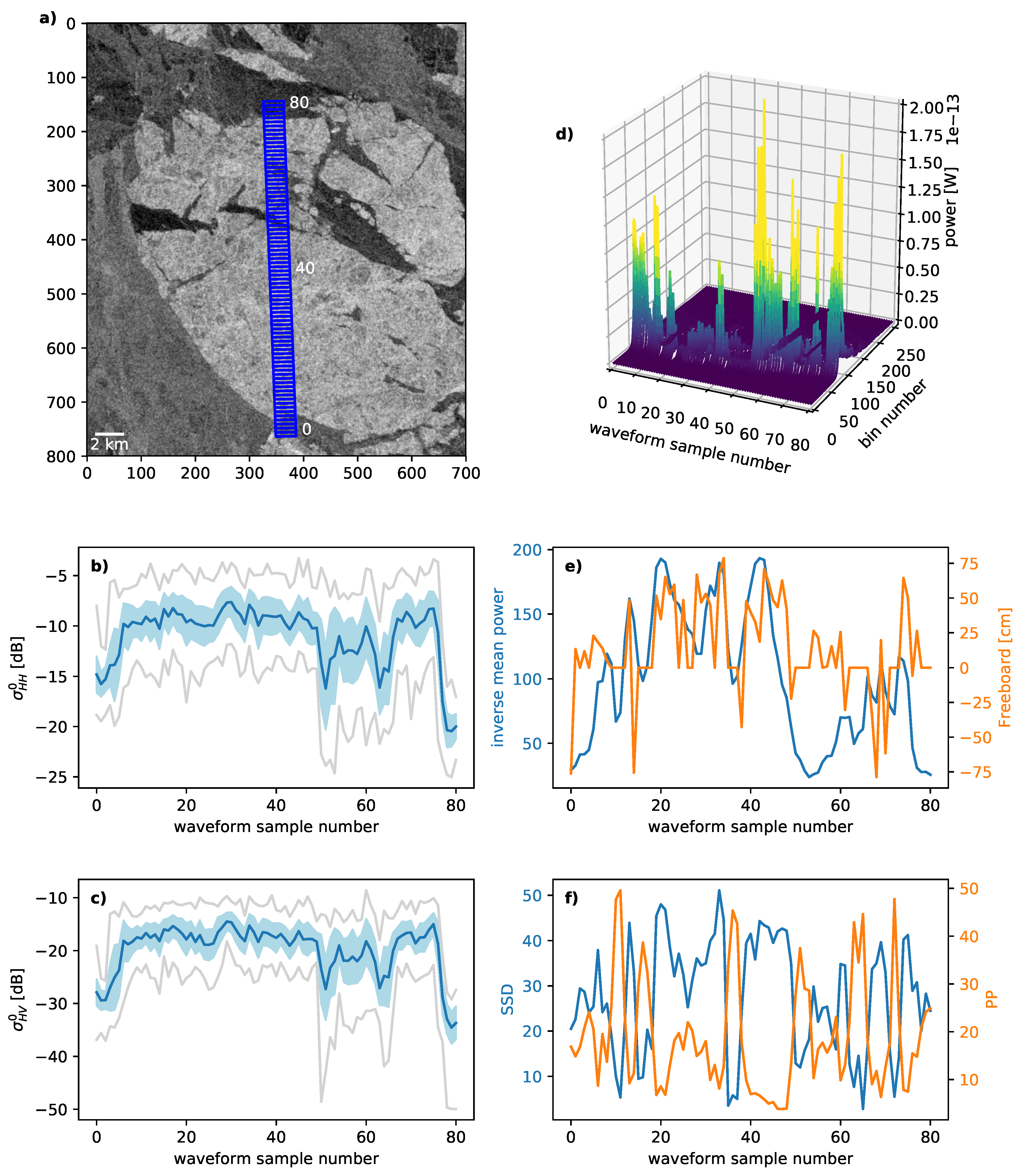
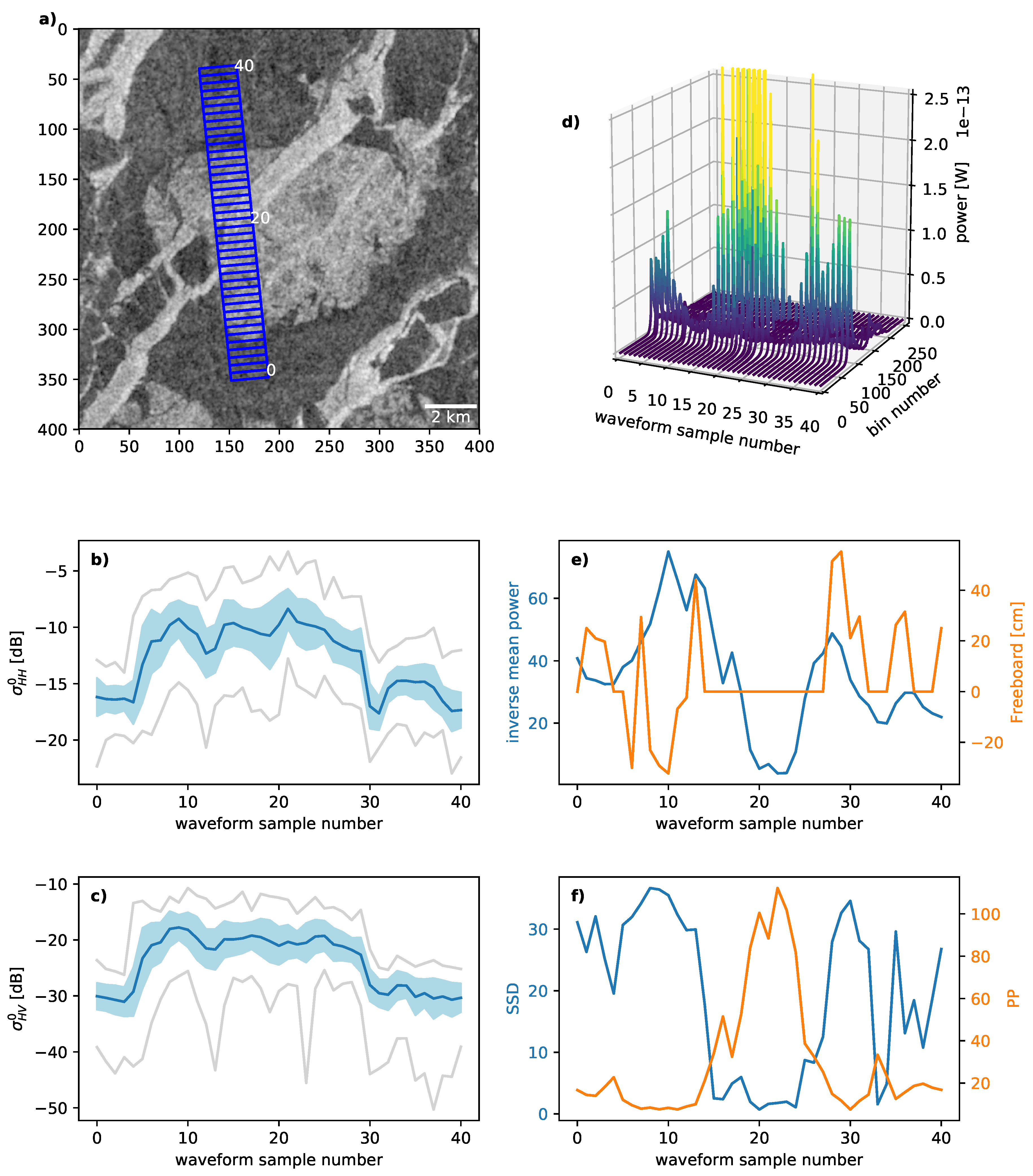
4.2. Local Waveform Variability

Of particular interest is the response of altimeter waveforms to spatial changes of the sea ice surface. In the following we present representative examples over a large ridge, and for different sized MYI floes that are embedded in FYI. Described findings are typical of these features and occurred for many samples in our dataset.

The first example in Figure 8 shows the local waveform variation and SAR imagery over a large ridge on 2016-03-15. The time lag between the SAR image and the altimeter track is below five minutes, i.e., for average drift speeds between 6 cm/s and 10 cm/s that means 18 m to 30 m. The ridge is clearly visible in the center of the cross-polarization SAR image by its higher backscatter caused by ice facets oriented towards the radar (Figure 8a–c). The altimeter on the other hand shows a lower peak intensity around the ridge because more energy is scattered away from the nadir-looking instrument (Figure 8d). PP is low over the ridge, while SSD and inverse mean power reach higher values (Figure 8e,f). This is characteristic for more diffuse scattering. Waveforms over FYI have a higher peak power with high PP and low SSD and inverse mean power. Notable is the large negative freeboard occurring for sample 25.

Figure 9 shows the waveforms in the vicinity of the negative freeboard and closer inspection of waveform 25 shows a multiple kinked leading edge towards the first peak that significantly delays the retracking point. The smoother sea ice areas, indicated by the darker tone in the SAR image, below the ridge begin to have an impact on the waveform and subsequent waveforms have an increased peak power. Observations over other ridges show that those features need to be sufficiently large, i.e., minimum 3 altimeter footprints, to not be affected by the more specular scattering of the FYI. The freeboard, expected to be larger over the ridge area, does, however, not show any significant changes compared to the surrounding FYI.

Figure 10 shows the SAR image and the spatial variation of altimeter waveforms of an old MYI floe embedded in thinner FYI. The data was taken on 22 February 2018 with a time separation of about 20 min, i.e., for average drift speeds between 6 cm/s and 10 cm/s that means 72 m to 120 m. The floe size along-track is approximately 24 km. In the SAR image, the MYI floe is characterized by high backscatter in co- and cross-polarization (Figure 10a) shows co-polarization) while the surrounding FYI has a lower backscatter. In the upper part of the MYI floe, some lead and low backscatter features are visible that are also reflected by reduced mean backscatter intensity and an increased standard deviation (light blue area in Figure 10b,c). The lower part of the floe looks relatively homogeneous. The waveforms in the interior of the floe show a low peak power with an exception around sample number 40 (Figure 10d). In this area the peak power is increased compared to before and after, but no feature is visible in the SAR image. The altimeter is very sensitive to smooth areas within the footprint that are too small to be resolved by the SAR but affect the measured waveform. Over the lower part of the MYI floe the freeboard estimate reflects the higher thickness of the MYI, but in the upper part of the floe, where smoother sea ice features affect the waveforms, freeboard is reduced. Therefore, in areas of mixed ice types sea ice freeboard more likely represents the smoother and thinner part of the ice. Negative freeboard is also observed in areas of changing sea ice surface at the beginning and end of the MYI floe. This example demonstrates the difficulties of obtaining robust freeboard even over relatively large and apparently homogeneous features, but careful observation of the changes in waveform shape facilitates explanation of the observations.

Figure 11 shows the SAR image and waveform spatial evolution over a small MYI floe that is split in two by a band of thinner ice with high SAR backscatter and smooth texture, i.e., brash ice or thin ice with a rough surface or frost flowers atop. The data was taken on 2018-02-24 with a time separation of about 10 min, i.e., for average drift speeds between 6 cm/s and 10 cm/s that means 36 m to 60 m. In the SAR image (Figure 11a) only the spatial context separates the MYI floe from the high backscatter FYI. A subtle difference between co- and cross-polarization channel mean backscatter can be observed. In the first one the backscatter around the feature is slightly increased, while for the latter one the backscatter is slightly decreased (Figure 11b,c around sample 20). The waveform peak power decreases with the start of the MYI floe but increases significantly over the thinner FYI area (Figure 11d)). That means that the FYI area must include areas of smooth ice, e.g., low density layer of frost flowers or open water between small flows that are responsible for the high power return. PP and SSD show only slight variations between the FYI before the floe and the MYI floe itself, while the difference in IMP is more pronounced (Figure 11e,f). The freeboard at the first part of the floe is mostly negative and only the smaller second part shows an increase of freeboard compared to the surrounding FYI.

The three presented test cases show that altimetric waveforms respond well to changes of the sea ice surface in the order of a few along-track altimeter footprints. Retrieval of a robust freeboard estimation of floes, however, requires significant larger features of a few kilometers to overcome uncertainties in estimating the surface elevation.

5. Discussion

Near-coincidental high-resolution SAR imagery significantly aids the interpretation of altimeter waveforms in particular for small-scale features in the sea ice cover. Waveform derived parameters such as PP, IMP and SSD can principally discern between FYI, MYI and leads. The sensitivity of altimeters waveforms to smooth areas within the footprint, however, complicates the classification task. We introduced the IMP parameter to improve the separability between FYI and MYI for cases where the peak power of the two ice types are similar (see Figure 4). Large temporal and spatial variability of these parameters, however, impedes the establishment of universally valid thresholds. Spatio-temporal changes can have a multitude of sources, e.g., differences in snow depth and composition [30,31], changes in surface roughness in the order of the radar wavelength [24] or temperature variations [32]. To circumvent this problem, adaptive thresholding has been proposed for larger scale assessments of ice type variability from altimeter data [7]. For small-scale investigations, the relative spatial evolution of waveforms corresponds well to changes of sea ice surface types as determined from SAR imagery (see Figure 8, Figure 9, Figure 10 and Figure 11). Therefore, usage of SAR imagery offers possibilities to assess the reasons of sea ice type misclassification from CryoSat-2 data [7,8] and inconsistencies in the spatial distribution of waveform parameters and sea ice type products [6] left unanswered in previous studies.

From the comparison of the altimeter data with the SAR images we observed that in areas of predominantly FYI, waveforms with high PP and peak power are common that are not linked to visible features in the SAR data. The increased peak power can be attributed to sub-resolution specular reflectors, e.g., thin smooth ice and leads that dominate the waveform. These findings are in line with observations from conventional (non-SAR) altimetry over the marginal ice zone [33]. Similarly, we found that in mixtures of FYI and MYI, waveforms tend to be more similar to FYI waveforms. The return from the smoother components are still strong enough to dominate the waveform in those cases. Difficulties in waveform interpretation over non-homogeneous surfaces are in accordance with earlier observations from Seasat data [15,34].

The complexity of altimeter waveform interpretation of mixed surfaces also showed an impact on freeboard estimates. Close to boundaries of distinct MYI floes in FYI, mixtures of ice types within a floe or small floes of MYI in FYI, freeboard estimates are lower compared to the interior of a homogeneous floe and similar to FYI freeboard measurements. While freeboard may vary over such a floe, this behavior is observed for nearly all floes in our study. Thus, the measurements most likely reflect the range to the thinner component either at nadir or off-nadir positions [35]. The latter ones often cause highly negative freeboard values because the range estimate is no longer associated with the nadir return. Underestimation of freeboard for mixed ice cases has been demonstrated in a simulation study based on CryoSat-2 parameters [36]. To reduce biases in freeboard retrievals due to ambiguous waveforms, returns with increased PP and peak power over FYI or waveforms with widened leading edge are usually discarded for sea ice thickness retrievals in standard gridded products [3,37]. Filtering of waveforms and spatial averaging reduces the effect of outliers but especially in the transition from FYI and MYI more research is necessary to quantify those effects on sea ice thickness retrievals. This is of great importance to reduce uncertainties in sea ice thickness estimates. While ambiguous waveforms introduce errors to freeboard estimates, local changes of sea ice characteristics leading to such irregular waveforms contain information about small-scale features of the sea ice surface.

Leads of thin ice or open water even smaller than the resolution of the SAR imagery are easily discerned by the altimeter due to their high PP and peak power. Caution needs to be taken to separate real leads and lead-like waveforms that are characterized by lower peak powers [38]. Lead detection is a necessary step in all sea ice freeboard retrievals and crucial to determine an optimal local sea surface height as a reference for the freeboard [39]. FYI within MYI floes most likely originates from refrozen leads or cracks in the ice and even small features are easily detected by waveform changes towards peakier more powerful returns. Freeboard estimates can be biased by off-nadir impact of the smoother reflectors [29,35]. Small-scale features with an increase in backscatter intensity in the SAR imagery, i.e., large ridges and old ice floes, are characterized by a decrease in PP and peak power in the altimeter waveform sequence. Features a few hundred meters in size can usually be identified but can only be unambiguously assigned to the correct cause by the SAR imagery. Freeboard measurements are, however, not significantly impacted by these small features compared to the surrounding FYI because of the reasons explained above for mixed ice cases. Acquisition of robust freeboard estimates over such features therefore requires this feature on the one hand to be large enough that the altimetric footprint is not affected by surrounding areas and on the other hand to provide enough valid freeboard measurements to obtain a meaningful average value. Based on the analysis of many MYI floes in our data set, we suggest that a floe size in the order of 10 km in along-track and a few kilometers to both sides across-track with a minimum of 10 valid freeboard measurements should act as a guideline for robust estimates of floe freeboard and hence ice thickness.

Altimetric waveforms can reflect small-scale changes of the sea ice surface in size scales from a fraction of the altimeter footprint for leads to a few hundred meters for ridges and old ice floes. The complexity of the waveform and the leading edge in particular introduced by non-homogeneous altimeter footprints, however, impede reliable freeboard estimates on these small scales. SAR imagery as additional data aids the interpretation of the altimeter data and facilitates the understanding of waveform responses to surface changes.

6. Conclusions

Using near-coincidental SAR imagery and altimetric data over three different winters in the Beaufort Sea, we showed that small-scale changes of a few hundred meters in sea ice surface related to leads, large ridges or ice floes of different sea ice types are recognizable by concurrent changes of altimetric waveforms. SAR imagery is a great asset to unambiguously identify the cause of these changes and to better understand the waveform behavior. SAR images thereby also facilitate the identification of regions potentially biased by the influence of thin ice features in older and thicker ice. Reliable freeboard estimates are possible for MYI floes in the order of 10 km in along-track and a few kilometers to both sides of the altimeter track. Freeboard estimates could be locally expanded to areas of similar signatures in the SAR image. The combination of information from SAR imagery and radar altimetry therefore has the potential to complete the picture of the sea ice situation on a local scale. SAR imagery however cannot solve the challenges imposed on freeboard to thickness retrieval by the properties of the snow layer [26], but improve the discrimination of ice types necessary for the calculation.

Retracking methods and selection procedures of valid waveforms for freeboard estimation have been optimized for hemispherical and basin-scale sea ice thickness retrieval [3,26]. Conversion of the here presented findings to useful additions to sea ice information from SAR imagery would benefit from the development of methods for locally optimized retrackers and improved waveform interpolation to better identify kinks in the leading edge of waveforms.

References

1. Dierking, W. Sea Ice Monitoring by Synthetic Aperture Radar. Oceanography 2013, 26. [Google Scholar] [CrossRef]
2. Ricker, R.; Hendricks, S.; Kaleschke, L.; Tian-Kunze, X.; King, J.; Haas, C. A weekly Arctic sea-ice thickness data record from merged CryoSat-2 and SMOS satellite data. Cryosphere 2017, 11, 1607–1623. [Google Scholar] [CrossRef] [Green Version]
3. Tilling, R.L.; Ridout, A.; Shepherd, A. Estimating Arctic sea ice thickness and volume using CryoSat-2 radar altimeter data. Adv. Space Res. 2018, 62, 1203–1225. [Google Scholar] [CrossRef]
4. Alexandrov, V.; Sandven, S.; Wahlin, J.; Johannessen, O.M. The relation between sea ice thickness and freeboard in the Arctic. Cryosphere 2010, 4, 373–380. [Google Scholar] [CrossRef] [Green Version]
5. Zygmuntowska, M.; Khvorostovsky, K.; Helm, V.; Sandven, S. Waveform classification of airborne synthetic aperture radar altimeter over Arctic sea ice. Cryosphere 2013, 7, 1315–1324. [Google Scholar] [CrossRef] [Green Version]
6. Zygmuntowska, M. Arctic Sea Ice Altimetry—Advances and Current Uncertainties. Ph.D. Thesis, University of Bergen, Bergen, Norway, 2014. [Google Scholar]
7. Rinne, E.; Similä, M. Utilisation of CryoSat-2 SAR altimeter in operational ice charting. Cryosphere 2016, 10, 121–131. [Google Scholar] [CrossRef] [Green Version]
8. Shen, X.; Zhang, J.; Zhang, X.; Meng, J.; Ke, C. Sea Ice Classification Using Cryosat-2 Altimeter Data by Optimal Classifier–Feature Assembly. IEEE Geosci. Remote Sens. Lett. 2017, 14, 1948–1952. [Google Scholar] [CrossRef]
9. Raney, R. The delay/Doppler radar altimeter. IEEE Trans. Geosci. Remote Sens. 1998, 36, 1578–1588. [Google Scholar] [CrossRef]
10. Wingham, D.; Francis, C.; Baker, S.; Bouzinac, C.; Brockley, D.; Cullen, R.; de Chateau-Thierry, P.; Laxon, S.; Mallow, U.; Mavrocordatos, C.; et al. CryoSat: A mission to determine the fluctuations in Earth’s land and marine ice fields. Adv. Space Res. 2006, 37, 841–871. [Google Scholar] [CrossRef]
11. Boy, F.; Desjonqueres, J.D.; Picot, N.; Moreau, T.; Raynal, M. CryoSat-2 SAR-Mode Over Oceans: Processing Methods, Global Assessment, and Benefits. IEEE Trans. Geosci. Remote Sens. 2017, 55, 148–158. [Google Scholar] [CrossRef]
12. Kildegaard Rose, S. Measurements of Sea ice by Satellite and Ariborne Altimetry. Ph.D. Thesis, DTU Space—National Space Institute, Lyngby, Denmark, 2013. [Google Scholar]
13. Passaro, M.; Müller, F.L.; Dettmering, D. Lead detection using Cryosat-2 delay-doppler processing and Sentinel-1 SAR images. Adv. Space Res. 2018, 62, 1610–1625. [Google Scholar] [CrossRef]
14. Longepe, N.; Thibaut, P.; Vadaine, R.; Poisson, J.C.; Guillot, A.; Boy, F.; Picot, N.; Borde, F. Comparative Evaluation of Sea Ice Lead Detection Based on SAR Imagery and Altimeter Data. IEEE Trans. Geosci. Remote Sens. 2019, 57, 4050–4061. [Google Scholar] [CrossRef]
15. Ulander, L.M.H. Interpretation of Seasat radar-altimeter data over sea ice using near-simultaneous SAR imagery. Int. J. Remote Sens. 1987, 8, 1679–1686. [Google Scholar] [CrossRef]
16. Fetterer, F.M.; Laxon, S.; Johnson, D.R. A comparison of Geosat altimeter and synthetic aperture radar measurements over east Greenland pack ice. Int. J. Remote Sens. 1991, 12, 569–583. [Google Scholar] [CrossRef]
17. Tilling, R.L.; Ridout, A.; Shepherd, A. Near-real-time Arctic sea ice thickness and volume from CryoSat-2. Cryosphere 2016, 10, 2003–2012. [Google Scholar] [CrossRef] [Green Version]
18. Karvonen, J.; Cheng, B.; Vihma, T.; Arkett, M.; Carrieres, T. A method for sea ice thickness and concentration analysis based on SAR data and a thermodynamic model. Cryosphere 2012, 6, 1507–1526. [Google Scholar] [CrossRef]
19. Laxon, S.W.; Giles, K.A.; Ridout, A.L.; Wingham, D.J.; Willatt, R.; Cullen, R.; Kwok, R.; Schweiger, A.; Zhang, J.; Haas, C.; et al. CryoSat-2 estimates of Arctic sea ice thickness and volume. Geophys. Res. Lett. 2013, 40, 732–737. [Google Scholar] [CrossRef] [Green Version]
20. Komarov, A.S.; Buehner, M. Detection of First-Year and Multi-Year Sea Ice from Dual-Polarization SAR Images Under Cold Conditions. IEEE Trans. Geosci. Remote Sens. 2019, 1–15. [Google Scholar] [CrossRef]
21. Kaur, S.; Ehn, J.K.; Barber, D.G. Pan-arctic winter drift speeds and changing patterns of sea ice motion: 1979–2015. Polar Rec. 2018, 54, 303–311. [Google Scholar] [CrossRef]
22. Scagliola, M. CryoSAT Footprints; Technical Report, Aresys Technical Note. 2013. Available online: https://earth.esa.int/documents/10174/125271/CryoSat_Footprints_TN_v1.1.pdf/2a5d996b-8b77-4d1c-ae7b-fbf93848c35d;jsessionid=B1FF8C50A1B0F2A0879F6FA028844644.eodisp-prod4040?version=1.0 (accessed on 29 September 2019).
23. European Space Agenncy. CryoSAT-2 Product Handbook; C2-LI-ACS-ESL-5319; European Space Agenncy: Paris, France, 2018. [Google Scholar]
24. Onstott, R.G. SAR and Scatterometer Signatures of Sea Ice. In Microwave Remote Sensing of Sea Ice; Carsey, F.D., Ed.; American Geophysical Union: Washington, DC, USA, 1992; Chapter 5; pp. 73–102. [Google Scholar]
25. Fetterer, F.M.; Drinkwater, M.R.; Jezek, K.J.; Laxon, S.W.C.; Onstott, R.G.; Ulander, L.M.H. Sea Ice Altimetry. In Microwave Remote Sensing of Sea Ice; Carsey, F.D., Ed.; American Geophysical Union: Washington, DC, USA, 1992; Chapter 7; pp. 111–135. [Google Scholar]
26. Ricker, R.; Hendricks, S.; Helm, V.; Skourup, H.; Davidson, M. Sensitivity of CryoSat-2 Arctic sea-ice freeboard and thickness on radar-waveform interpretation. Cryosphere 2014, 8, 1607–1622. [Google Scholar] [CrossRef] [Green Version]
27. Quartly, G.D.; Rinne, E.; Passaro, M.; Andersen, O.B.; Dinardo, S.; Fleury, S.; Guillot, A.; Hendricks, S.; Kurekin, A.A.; Müller, F.L.; et al. Retrieving Sea Level and Freeboard in the Arctic: A Review of Current Radar Altimetry Methodologies and Future Perspectives. Remote Sens. 2019, 11, 881. [Google Scholar] [CrossRef]
28. Brockley, D.J. CryoSat2: L2 Design Summary Document; CS-DD-MSL-GS-2002; 2019. Available online: https://earth.esa.int/documents/10174/125272/CryoSat-L2-Design-Summary-Document (accessed on 29 September 2019).
29. Landy, J.C.; Tsamados, M.; Scharien, R.K. A Facet-Based Numerical Model for Simulating SAR Altimeter Echoes From Heterogeneous Sea Ice Surfaces. IEEE Trans. Geosci. Remote Sens. 2019, 57, 4164–4180. [Google Scholar] [CrossRef] [Green Version]
30. Ricker, R.; Hendricks, S.; Perovich, D.K.; Helm, V.; Gerdes, R. Impact of snow accumulation on CryoSat-2 range retrievals over Arctic sea ice: An observational approach with buoy data. Geophys. Res. Lett. 2015, 42, 4447–4455. [Google Scholar] [CrossRef]
31. Fons, S.W.; Kurtz, N.T. Retrieval of snow freeboard of Antarctic sea ice using waveform fitting of CryoSat-2 returns. Cryosphere 2019, 13, 861–878. [Google Scholar] [CrossRef] [Green Version]
32. Nilsson, J.; Vallelonga, P.; Simonsen, S.B.; Sørensen, L.S.; Forsberg, R.; Dahl-Jensen, D.; Hirabayashi, M.; Goto-Azuma, K.; Hvidberg, C.S.; Kjær, H.A.; et al. Greenland 2012 melt event effects on CryoSat-2 radar altimetry. Geophys. Res. Lett. 2015, 42, 3919–3926. [Google Scholar] [CrossRef]
33. Drinkwater, M.R. Ku-band airborne radar altimeter observations of marginal sea ice during the 1984 Marginal Ice Zone Experiment. J. Geophys. Res. 1991, 96, 4555. [Google Scholar] [CrossRef]
34. Ulander, L. Observations Of Ice Types In Satellite Altimeter Data. In Proceedings of the International Geoscience and Remote Sensing Symposium, Remote Sensing: Moving Toward the 21st Century, Edinburgh, UK, 12–16 September 1988. [Google Scholar] [CrossRef]
35. Armitage, T.W.K.; Davidson, M.W.J. Using the Interferometric Capabilities of the ESA CryoSat-2 Mission to Improve the Accuracy of Sea Ice Freeboard Retrievals. IEEE Trans. Geosci. Remote Sens. 2014, 52, 529–536. [Google Scholar] [CrossRef]
36. Tonboe, R.T.; Pedersen, L.T.; Haas, C. Simulation of the CryoSat-2 satellite radar altimeter sea ice thickness retrieval uncertainty. Can. J. Remote Sens. 2010, 36, 55–67. [Google Scholar] [CrossRef] [Green Version]
37. Ricker, R.; Hendricks, S.; Helm, V.; Gerdes, R. Classification of CryoSat-2 Radar Echoes. In Towards an Interdisciplinary Approach in Earth System Science: Advances of a Helmholtz Graduate Research School; Lohmann, G., Meggers, H., Unnithan, V., Wolf-Gladrow, D., Notholt, J., Bracher, A., Eds.; Springer International Publishing: Cham, Switzerland, 2015; pp. 149–158. [Google Scholar] [CrossRef] [Green Version]
38. Wernecke, A.; Kaleschke, L. Lead detection in Arctic sea ice from CryoSat-2: Quality assessment, lead area fraction and width distribution. Cryosphere 2015, 9, 1955–1968. [Google Scholar] [CrossRef]
39. Kwok, R.; Cunningham, G.F. Variability of Arctic sea ice thickness and volume from CryoSat-2. Philos. Trans. R. Soc. A Math. Phys. Eng. Sci. 2015, 373, 20140157. [Google Scholar] [CrossRef]
Figure 1. Beaufort Sea study area: Sentinel-1 images are shown in blue and the red lines represent the CryoSat-2 altimeter ground tracks. The inset in the upper left corner shows the location of the study area in the Arctic.
Remotesensing 11 02602 g001
Figure 2. Example waveforms for different surface types. (a) Lead, (b) first-year and (c) multiyear sea ice. Note the difference in the scaling of the y-axis.
Remotesensing 11 02602 g002
Figure 3. Example of waveform evolution over a multiyear sea ice floe 2018-02-18. (a) HV SAR image with altimeter footprint in blue rectangles [Contains Copernicus Sentinel data 2018] and (b) waveforms in different colors for distinction and freeboard as a solid black line.
Remotesensing 11 02602 g003
Figure 4. Waveform parameters of different ice types covering all winter seasons. (a) Pulse peakiness, (b) scaled mean power, (c) stack standard deviation and (d) mean HV backscatter intensities of altimeter footprint. Solid lines represent a kernel density estimate from measured histograms.
Remotesensing 11 02602 g004
Figure 5. Waveform parameters of FYI for the different winter seasons. (a) Pulse peakiness, (b) scaled mean power, (c) stack standard deviation and (d) mean HV backscatter intensities of altimeter footprint. Solid lines represent a kernel density estimate from measured histograms.
Remotesensing 11 02602 g005
Figure 6. Waveform parameters of MYI for the different winter seasons. (a) Pulse peakiness, (b) scaled mean power, (c) stack standard deviation and (d) mean HV backscatter intensities of altimeter footprint. Solid lines represent a kernel density estimate from measured histograms.
Remotesensing 11 02602 g006
Figure 7. Freeboard distributions for (a) FYI and MYI of all winter seasons, (b) FYI and (c) MYI for the three winter seasons. Solid lines are kernel density estimates of the histograms.
Remotesensing 11 02602 g007
Figure 8. Waveform evolution and SAR imagery over a large ridge feature on 2016-03-15 with time separation less than five minutes. (a) SAR HV image with blue rectangles marking the altimeter footprints, (b,c) HH and HV mean backscatter with standard deviation interval in light blue and minimum and maximum values in grey, (d) waveforms, (e) mean inverse power and freeboard and (f) SSD and PP. [Contains Copernicus Sentinel data 2016]
Remotesensing 11 02602 g008
Figure 9. Evolution of waveforms over the ridge in vicinity of the large negative freeboard value.
Remotesensing 11 02602 g009
Figure 10. Waveform evolution and SAR imagery over a large MYI floe on 22 February 2018 with time separation of about 20 min. (a) SAR HH image with blue rectangles marking the altimeter footprints, (b,c) HH and HV mean backscatter with standard deviation interval in light blue and minimum and maximum values in grey, (d) waveforms, (e) mean inverse power and freeboard and (f) SSD and PP. [Contains Copernicus Sentinel data 2018]
Remotesensing 11 02602 g010
Figure 11. Waveform evolution and SAR imagery over a small MYI floe embedded in FYI on 2018-02-24 with time separation of about 10 min. The small MYI floe is split in two by a high backscatter FYI feature. (a) SAR HV image with blue rectangles marking the altimeter footprints, (b,c) HH and HV mean backscatter with standard deviation interval in light blue and minimum and maximum values in grey, (d) waveforms, (e) mean inverse power and freeboard and (f) SSD and PP. [Contains Copernicus Sentinel data 2018]
Remotesensing 11 02602 g011