A Rapidly Assessed Wetland Stress Index (RAWSI) Using Landsat 8 and Sentinel-1 Radar Data

Abstract

Wetland ecosystems are important resources, providing great economic benefits for surrounding communities. In this study, we developed a new stress indicator called “Rapidly Assessed Wetlands Stress Index” (RAWSI) by combining several natural and anthropogenic stressors of wetlands in Delaware, in the United States. We compared two machine-learning algorithms, support vector machine (SVM) and random forest (RF), to quantify wetland stress by classifying satellite images from Landsat 8 and Sentinel-1 Synthetic Aperture Radar (SAR). An accuracy assessment showed that the combination of Landsat 8 and Sentinel SAR data had the highest overall accuracy (93.7%) when used with an RF classifier. In addition to the land-cover classification, a trend analysis of the normalized difference vegetation index (NDVI) calculated from Landsat images during 2004–2018 was used to assess changes in healthy vegetation. We also calculated the stream sinuosity to assess human alterations to hydrology. We then used these three metrics to develop RAWSI, and to quantify and map wetland stress due to human alteration of the landscape. Hot-spot analysis using Global Moran’s I and Getis-Ord Gi* identified several statistically significant hot spots (high stress) in forested wetlands and cold spots (low values) in non-forested wetlands. This information can be utilized to identify wetland areas in need of further regulation, with implications in environmental planning and policy decisions.

1. Introduction

The Environmental Protection Agency (EPA) defines wetlands as “areas in which water covers the soil, or is present at or near the surface of the soil all year or for varying periods of time during a year, including during the growing season” [1], yet, “wetlands” is a broad term and might have varied characteristics in terms of hydrology, vegetation, and soils. To standardize the classification of wetlands, a classification system was developed by the United States Fish and Wildlife Service (FWS) and adopted by several agencies within the United States government. This system broadly categorizes wetlands into marine, estuarine, riverine, lacustrine, and palustrine wetlands [2].

Wetlands are the most productive ecosystems in the world, providing ecosystem services that benefit humans, such as provision of food, water regulation, aquatic habitat, recreation, and tourism [3,4,5,6,7,8,9,10]. Wetland ecosystem services provide an estimated $4.9 trillion worth of services annually across the globe [11]. Wetlands also play a vital role in climate change mitigation through carbon sequestration [12]. Despite the value and importance of wetlands, large-scale wetland loss and degradation has been affecting the overall health of wetlands for hundreds of years, leading to the loss of ecosystem services. It has been estimated that 50% of wetlands have been lost globally since 1900; however, a more recent review estimated a loss of between 64% and 71%, with greater amounts of loss occurring in inland wetlands [13,14]. Common factors that lead to degradation of wetlands include eutrophication from urban and agricultural lands, invasive plants, hydrologic alterations, salinization, and filling, while wetland loss is typically a result of conversion of land use and drainage for agriculture [15].

Such loss in ecosystem services is a particularly critical environmental issue in a coastal state such as Delaware. Around 25% of Delaware is covered by different wetland types, such as salt marshes, bays, and freshwater wetlands [16]. Important ecosystem services are provided by these wetlands, such as improving water quality, reducing flood occurrences, providing plant and animal habitat, and providing educational and recreational opportunities. Wetlands in Delaware face many impacts from natural events such as subsidence and storms, but also experience impacts from human activities such as nutrient loading, stream channelization, drainage for agriculture and flood control, urban development, dredging of channels, timber harvest, ground-water extraction, and pollution [17]. These events or activities that negatively affect wetlands are considered stressors.

The objective of this paper is to focus on human-induced stressors, such as development of land, destruction of vegetation, and alterations in hydrology, as these factors are commonly used in the evaluation of wetlands and can be observed at a landscape scale. The Delaware Rapid Assessment (DERAP) is an example of a wetland-assessment method, assessing wetland conditions based on the total number of stressors within a site, primarily based on field observations rather than remote sensing [18]. DERAP breaks down these stressors into three categories: habitat/plant community, hydrology, and landscape buffer [19]. A similar wetland assessment method is the EPA Level 2 assessment, which is a rapid assessment method based on hydrology, soils/substrate, vegetation, and landscape setting [20]. The EPA also has a Level 1 assessment method that uses landscape-level remote-sensing data, rather than field data, to assess wetland conditions more broadly.

Currently, even rapid assessments, such as DERAP and EPA Level 2, require time, expertise, and equipment, among other resources. The development of a wetland assessment index similar to DERAP and EPA Level 2 that is based on methods more similar to the EPA Level 1 assessment, such as the use of remote sensing and ancillary geographic data, would have the potential to allow for the automation of wetland assessments. Through the use of remotely sensed data, the drawbacks of rapid assessment methods are minimized, as multiple wetland areas can be assessed simultaneously. Additionally, the use of remotely sensed data allows for large areas of wetlands, including those on private lands, to be assessed, which would otherwise not be possible. However, remote-sensing methods have their own disadvantages, such as the lack of information due to limited spectral and spatial resolutions.

Prior studies on wetland remote sensing involve the classification of wetland types with the goal of producing highly accurate wetland maps using hyperspectral and high spatial resolution imagery, including aerial photography [21,22,23,24,25]. Rather than identifying wetland types or measuring wetland loss with aerial photography and hyperspectral data, this work uses freely available data, such as Landsat, Sentinel imagery, and United States Geological Survey (USGS) stream data, in an attempt to create a method of assessing wetland health that is robust and easily reproducible. While a wetlands dataset, the National Wetlands Inventory (NWI), already exists, this dataset has known limitations, such as low temporal resolution (updated every 10 years) and underestimation of wetlands [26]. Other land-cover maps for Delaware contain more general wetland classes, such as the 2007 classification developed by Aerial Information Systems [27]. However, an up-to-date dataset classifying wetlands and other land covers does not exist.

While there are many stressors that can impact a wetland, we developed an index that quantifies the most prevalent stressors that have the biggest impact on Delaware wetland conditions based on wetland reports and evaluation methods specific to the state [18]. The metrics used in our index include land cover adjacent to wetlands, change in natural vegetation, and channelization of streams.

We evaluated two machine-learning algorithms, Random Forest (RF) and Support Vector Machine (SVM) to answer the following questions:

• Which classification method, between RF and SVM, provides the highest mapping accuracy for Delaware wetlands?
• How does wetland stress vary across Delaware, both spatially and by wetland type?

2. Materials and Methods

2.1. Study Area

The state of Delaware spans over an area of 6446 km² and hosts a population of almost 1 million people. The state contains a large amount of farmland and urban areas, such as the City of Wilmington. The majority of the coastline is connected to the Delaware Bay; however, a portion of the southern region is connected to the Atlantic Ocean. Delaware has an overall low elevation, close to sea level, with a maximum elevation of 137 m. The mean elevation in Delaware is lower than any other US state, with an average of 18 m above sea level. Due to this low elevation and large coastline, Delaware has several types of tidal and nontidal wetlands [2,17]. The state has a moderate climate year-round, with mean monthly temperatures ranging from 0 to 24.3 degrees Celsius and approximately 1143 mm of rainfall annually. Delaware consists of three counties: New Castle, Kent, and Sussex (Figure 1). Southern areas tend to be dominated by agriculture, while northern areas contain more urban and suburban areas.

2.2. Land-Cover Classification

Two classifications methods, RF and SVM, are compared in this study, using eight broad land-cover classes. Landsat 8 Tier 1 Top of Atmosphere (TOA) Reflectance data provided by the United States Geological Survey (USGS) and Sentinel-1 Synthetic Aperture Radar (SAR) satellite imagery provided by the European Space Agency (ESA) were used for the land-cover classification of Delaware. Landsat 8 imagery has been heavily used for land-cover applications, such as crop and wetland identification, since its launch in 2013, due to its moderate spatial resolution (30 m) and global coverage [28,29,30,31,32]. However, as Landsat cannot accurately capture signals within dense foliage and soil, wetlands that are covered by dense forests or with water just below the surface cannot be accurately identified using Landsat imagery alone. To increase wetland classification accuracy, several studies have utilized SAR data, often by combining it with optical data, as it can penetrate into dense foliage and soil, leading to better classification of dynamic wetlands [33,34,35,36,37,38,39,40,41,42,43]. To capture conditions existing outside Delaware that may still be affecting Delaware wetlands, a 300-meter buffer around the state boundary was used to clip all of the satellite images used for classification.

2.2.1. Satellite Data

Classification algorithms and remote sensing data used in this study were accessed and processed on the Google Earth Engine (GEE) platform. GEE is a cloud-based geospatial processing platform that provides access to machine-learning algorithms, such as RF, SVM, and Classification and Regression Trees (CART), that are known to provide high classification accuracy [44,45]. Additionally, GEE allows for results to be easily reproduced, as the platform is free, can analyze data for large study areas, and is script-based.

All 69 Landsat 8 Tier 1 TOA reflectance images captured over the study area during the 2018 calendar year were used to consider the most recent conditions and account for annual variation in crops and other vegetation [46]. A cloud mask was applied to all images within this dataset, using Bit 4 of the Quality Assessment band (BQA). Pixels with a nonzero value were masked, as those pixels contained clouds. Bands 2 (Blue), 3 (Green), 4 (Red), 5 (Near Infrared), 6 (Shortwave Infrared 1), 7 (Shortwave Infrared 2), 10 (Thermal 1), and 11 (Thermal 2) were selected to include optical and thermal information that is useful in differentiating land-cover types. GEE provides access to resampled Bands 10 and 11 (from 100 to 30 m resolution) to be compatible with bands 2–7. The median value for each band was calculated for every pixel location, using all Landsat images captured throughout the year. This method provides an image capturing average conditions, with less influence from outlying values, and is commonly used when studying land cover within GEE [47,48,49,50,51,52,53,54,55].

The SAR data in this study are from the Sentinel-1 C-band. This dataset within GEE was preprocessed, using Ground Range Detected (GRD) border-noise removal, thermal noise removal, radiometric calibration, and terrain correction, to derive backscatter coefficients [56]. The Sentinel-1 C-band is used because this dataset is free and easily accessible in GEE. We filtered the instrument mode to consider the Interferometric Wide Swath (IWS), which is generally used for land characterization [57]. We also set the transmitter receiver polarization to vertical transmit and vertical receive (VV), which is suitable for wetland monitoring [58]. The SAR images were then filtered for three seasons, spring (April through June), summer (July through September), and fall (October through December), to capture the decrease in wetland backscatter within SAR imagery, from spring to fall [34]. A median image was derived for SAR images in each of these three seasons. A composite of this seasonal SAR data and the Landsat 8 data was then created by stacking all the bands selected from Landsat 8 with the three seasonal composite bands from Sentinel-1 into one image. The spatial resolution of the Sentinel-1 image was resampled to match the resolution of the Landsat 8 image (30 m).

2.2.2. Classification Method

We compared 4 classification methods to determine which provided the highest overall and per-class accuracy, specifically for wetland classes, for further use in our study. An RF and SVM classification with Landsat 8 and Sentinel-1 SAR data, and with just Landsat 8 data, were tested. We compared these two classifiers because these are prevalent classification algorithms used in similar studies [59,60,61,62,63,64], and they are easily implementable on GEE. RF and SVM are supervised classification methods that rely on a machine-learning approach [59,60,61,65,66,67]. Studies that were conducted, comparing RF and SVM, generally show a higher accuracy with SVM [62,63,64]. However, we wanted to compare available methods to achieve the highest possible accuracy for our study area.

RF works by using an ensemble of uncorrelated decision trees to make a decision; trees are kept uncorrelated by using a bagging method in which decision trees randomly sample from a dataset [68]. It is necessary to reduce the number of decision trees through the process of pruning, in order to generate more accurate results [69]. On the other hand, SVM classifiers use a plotted hyperplane to separate class values and are based on different kernel types, such as polynomials, splines, and radial-basis functions (RBF) [70]. While other classification methods, such as unsupervised or hybrid methods were shown to be effective, we used a supervised method in our land-cover classification, in order to have control over what classes were being selected [71,72,73].

For the RF classification, the number of trees used was 100, as a prior study indicated that more than 128 trees result in little to no performance gain [74]. The remaining parameters, i.e., variables per split, minimum leaf population, bag fraction, out-of-bag mode, and seed, were set at their default values: 0 (defaults to the square root of the number of variables), 1, 0.5, false, and 0 (random seed), respectively. The following parameters were used for our SVM classification: kernel type, RBF; gamma, 0.5; and cost, 10.

2.2.3. Land-Cover Types

The land-cover types used in this classification are based on those developed by Anderson et al. [75]. This classification scheme uses a hierarchical standardized approach based on broad Level 1 classes that are further broken down into more specific Level 2 classes. The Level 1 land covers used in this study are described in

Table 1. The land-cover types based on Anderson’s Classification System developed for the United States Geological Survey (USGS), and number of reference points (collected using high-resolution imagery) used in this study for the image classification and validation.

Land Cover	Description	Number of Reference Points
Built	Land developed with impervious surfaces, such as roads, buildings, or parking lots, even if covered by other land covers, such as grass or trees	500
Cropland	Fields used for growing and harvesting crops	350
Barren	Includes areas with bare soil year-round, such as sand or industrial fields	150
Forest	Any area predominantly covered in trees and not water	100
Water	Any area covered by water year-round	200
Forested Wetland	Any forested area that is at least periodically covered by water	200
Non-Forested Wetland	Areas that are at least periodically covered in water and contain grasses and other wetland plants	150
Shrubland	Areas covered in shrubs and without water	100

. We further broke down the wetlands class in the Anderson Level 1 classification scheme into forested and non-forested wetlands. This was necessary for wetlands within forested areas to still be classified as wetlands rather than forests. We used the broad Anderson Level 1 classes in order to simplify the classification, to make it easily reproducible, while only providing necessary information for a wetland stress index.

2.2.4. Reference Data

A total of 1750 reference points were collected across the study area, using high-resolution satellite imagery from 2018, accessed on Google Earth Pro (Table 1). Wetland-area reference points were identified using both Google Earth Pro Satellite Imagery and Sentinel-1 SAR imagery within Delaware. The use of Sentinel-1 SAR data facilitated identification of forested wetland areas that are difficult to identify with optical imagery due to tree cover. The number of reference points chosen for each class was based on the proportion of each land cover within the study area, as assessed by a visual estimate. We used these reference points to extract spectral information from the minimum sample unit, i.e., pixels.

2.2.5. Post-Processing

The RF and SVM classifications resulted in many singular improperly classified pixels or noise, as identified through visual inspection. To remove this noise, a majority filter (3 × 3 window) was used. This filter identifies eight neighboring pixels for each pixel, using a moving window, and reclassifies the pixel as the majority value of the neighboring pixels [76]. To exclude land covers that would have little to no effect on wetland condition, a buffer of 150 m was applied to the wetland classes (water, forested wetland, and non-forested wetland) identified in the 2018 land-cover classification. We used 150 m as the buffer criteria, based on the EPA Level 2 Rapid Assessment that determines landscape setting based on the dominant land use within 150 m of a wetland and the range of 3–200 m of surrounding land that was determined to impact a variety of different wetlands [20,77]. Only land covers within this buffer were used for the assessment. We used ArcGIS Pro version 2.2.0 for the post-processing.

2.2.6. Accuracy Assessment

To assess the accuracy of the classification, 60% of reference points (Table 1) were used to train the classifier, and 40% were used to test the accuracy of the predictions. A confusion matrix was produced, and the total number of points correctly predicted was divided by the total number of test points to calculate the overall accuracy. In addition, we calculated user’s accuracy, producer’s accuracy, and a kappa coefficient [78,79].

2.3. Natural-Vegetation Change Detection

In this study, natural vegetation is defined as areas containing forest or wetland plants. This metric does not include lawns or crop fields. In this study, a timespan of 15 years (2004–2018) was used to understand how vegetation within and surrounding wetlands changed over time. We used a hybrid classification to determine areas that witnessed changes in natural vegetation. A hybrid classification was used because of the lack of training data from earlier years. Landsat 5 and 8 were used to examine vegetation cover during 2004–2012 and 2013–2018, respectively. An annual median composite was derived for each year between 2004 and 2018. Cloudy pixels were excluded from the median composite. We used a K-means clustering algorithm for the unsupervised classification available in GEE [80,81]. This method was initially implemented with 20 clusters. We then manually examined the 20 clusters for each year and selected and merged the clusters representing naturally vegetated areas, creating maps of naturally vegetated areas for each year. We then calculated NDVI for each year, based on the Landsat 5 and 8 median cloud-free composites, and clipped to the extent of the natural vegetation class. This step enabled us to quantify changes within natural vegetation. NDVI is a proxy for vegetation health, based on the greenness of a pixel, using near infrared (NIR) and red bands of the satellite sensors. NDVI is calculated using the following equation:

NDVI = (NIR − Red)/(NIR + Red)

(1)

NDVI is effectively used in quantifying vegetation change using time series data [82,83]. We used a generalized linear regression model in RStudio version 3.6 to determine the trend of annual NDVI over 15 years. Additionally, significance of this trend, using an F-test, was calculated.

2.4. Stream Channelization

Channelized streams were identified by measuring the sinuosity index of every stream within the Delaware Flowlines Dataset provided by the USGS National Hydrography Dataset. This dataset provides a vector layer of streams and has many applications for hydrological research [84]. A sinuosity index is measured for each stream segment, representing the meander of a stream [85]. This is measured by dividing the stream length by the length of a straight line between the beginning and end point of the stream [86]. We calculated the sinuosity ratio, using ArcGIS Pro version 2.2.0. In general, a lower sinuosity, close to 1, represents more anthropogenic influence and lower stream health, while higher sinuosity values represent greater meandering, as seen in non-channelized streams. A threshold sinuosity index of 1.05 was used in this study to determine if a stream was channelized [87].

2.5. Rapidly Assessed Wetland Stress Index (RAWSI)

While many anthropogenic activities result in wetland stress, we attempted to select criteria that have the most effects on wetlands. To do this, we adopted some of the DERAP criteria, as those are widely used by wetland experts in Delaware and were calibrated using data within Delaware. Approximately 66% of metrics from DERAP are represented in the wetland stress index developed in this study, either directly or indirectly, as shown in

Table 2. Table of Delaware Rapid Assessment (DERAP) metrics [18]. Metrics in dark gray represent those directly measured by the Rapidly Assessed Wetland Stress Index (RAWSI) developed in this study. Metrics in light grey are expected to influence the RAWSI metrics indirectly. Metrics in white are not represented in RAWSI.

Habitat/Plant Community	Hydrology	Landscape Buffer
Mowing	Ditching	Development (residential)
Farmed	Channelized Streams	Development (commercial)
Grazing	Weir/Dam/Road	Sewage Disposal
Forest harvest	Stormwater Inputs	Septic Disposal
Cleared Land	Point Sources	Trails
Excessive Herbivory	Filling, Excavation	Roads
Invasive Species	Microtopographic Alteration	Landfill
Chemical Defoliation	Soil Subsidence	Agriculture (row crops)
Pine Conversion	Tidal Restriction	Agriculture (orchards)
Burned		Agriculture (poultry)
Trails		Forest Harvest
Garbage/Dumping		Marinas
Increased Nutrients		Golf Course
Roads		Mowed
		Sand/Gravel Mining

. All these metrics can be calculated in an automated way, using satellite imagery on an annual or seasonal basis; hence, we named it Rapidly Assessed Wetland Stress Index (RAWSI).

Our land-cover classification directly identifies developed (built), forests, agriculture (crop fields), and sand (barren land). Furthermore, roads, trails, landfills, and marinas all contain impervious cover and are thus classified as built areas. Golf courses and mowed areas commonly contain spectral signatures similar to agriculture, so they are generally classified as crop fields by our classifier. Forest harvest and vegetation alterations are considered in RAWSI by assessing natural-vegetation change. Channelized streams are directly included in our study and include impacts of other anthropogenic hydrologic alterations, such as dams and ditching.

Wetland pixels were combined into wetland areas by the connectedness of pixels and similar types of wetlands, using ArcGIS Pro. These similar and connected wetland areas are used for assessment in RAWSI, with each wetland area given one stress value in the RAWSI index. A total of 41,172 wetland areas were identified in Delaware with our land-cover classification. To assess the influence of land cover on a wetland, the percentage of a wetland buffer (within 150 m) that is covered by built and cropland was calculated. Vegetation loss was assessed per wetland by determining the percentage of the wetlands and wetland buffers that experienced any degree of NDVI loss (with a negative trend as identified by the regression analysis) over the past 15 years. All NDVI loss (irrespective of statistical significance) was treated equally in this index because the timescale used was too short to yield statistical significance. Hydrology was assessed by determining the ratio of channelized stream length to overall stream length within a wetland area. Wetland areas with no streams have a value of zero for hydrologic stress. To standardize these metrics (Table 2), each was rescaled to values from 1 to 100, based on the quantile that a pixel value fell within when compared to the entire dataset for that metric. To create an overall index for wetland stress, the rescaled values for human-influenced land cover, vegetation loss, and stream channelization were averaged for all wetland areas (water, non-forested wetland, and forested wetland). The wetland stress index values range between 0 and 100.

2.6. Spatial Patterns in RAWSI

To measure the spatial patterns within the RAWSI dataset, two statistical tests were used: Global Moran’s I and Getis-Ord Gi*. Global Moran’s I is a measure of spatial autocorrelation calculated across an entire dataset that determines if a dataset is significantly dispersed, random, or clustered and calculates a feature’s deviation from the mean and creates a cross product with neighboring features [88]. A negative value in the Global Moran’s Statistic denotes dispersion, while positive values represent clustering. A Z-score and p-value are also computed to determine if the Global Moran’s I statistic is significant for the dataset. The Getis-Ord Gi* statistic is used to identify significant spatial clusters of high (hot spots) and low values (cold spots) by calculating the Gi* statistic for each wetland feature [89]. Each feature is compared to each neighboring feature: high values surrounded by high values are considered hot spots, and low values surrounded by low values are considered cold spots. This statistic is calculated by comparing the actual local sum to the expected local sum with a significance test. The neighborhood search threshold for both statistics was 1182.14 m, as this is the largest distance between a wetland feature and its nearest neighbor in the dataset, and we needed to ensure each feature had at least one neighbor. Both of the statistics were calculated in ArcGIS Pro version 2.2.0.

3. Results

3.1. Spatial Distribution of Land Covers within Delaware

The combination of Sentinel-1 SAR with Landsat 8 data shows slightly greater accuracy when compared to the use of only Landsat data in the RF classification, with overall accuracy increasing from 92.7% to 93.7% and kappa coefficient increasing from 0.912 to 0.924 (

Table 3. Classification accuracies for each classification type that was attempted in this study, using Random Forest (RF) and Support Vector Machine (SVM).

Classification Type	User’s Accuracy	Producer’s Accuracy	Overall Accuracy	Kappa
Landsat 8 and Sentinel-1 RF			93.7%	0.924
Forest	91.4%	96.9%
Water	98.5%	100%
Built	92.8%	96.5%
Crop Fields	90.4%	94%
Barren	91.8%	84.9%
Non-Forested Wetland	93.7%	100%
Forested Wetland	100%	86.2%
Rangeland	100%	75.7%
Landsat 8 RF			92.7%	0.912
Forest	93.9%	93.9%
Water	98.5%	100%
Built	92.7%	95.9%
Crop Fields	86.2%	93%
Barren	91.4%	81.1%
Non-Forested Wetland	97.8%	100%
Forested Wetland	96.4%	93.1%
Rangeland	92%	69.6%
Landsat 8 and Sentinel-1 SVM			70%	0.63
Forest	64.8%	72.7%
Water	100%	91.3%
Built	65.4%	87.7%
Crop Fields	71.8%	78.2%
Barren	58.3%	26.4%
Non-Forested Wetland	61.2%	42.2%
Forested Wetland	66.6%	62%
Rangeland	52.3%	33.3%
Landsat 8 SVM			79.4%	0.752
Forest	84%	63.6%
Water	95.8%	100%
Built	83.6%	83.6%
Crop Fields	71.7%	83.1%
Barren	88%	69.8%
Non-Forested Wetland	88.8%	88.8%
Forested Wetland	54.7%	79.3%
Rangeland	40%	24.2%

). Both RF-derived classifications, with and without Sentinel-1 data, resulted in a considerable increase in accuracy over both SVM-derived classifications, which had an overall accuracy of 79.4% and 70%, without and with Sentinel-1 data, respectively. Some of the improved accuracy when including the Sentinel-1 data into the RF classification came from the forested wetland class, of which the user’s accuracy increased from 96.4% to 100%. However, the use of Sentinel-1 data led to a slight decrease in non-forested wetland accuracy, with user’s accuracy decreasing from 97.8% to 93.7%. This decrease is due to non-forested wetlands being classified either as forested wetlands or rangeland.

We used the RF classification with Landsat 8 and Sentinel-1 data to calculate RAWSI, as it has the highest overall accuracy. According to this RF-derived classification (Figure 2c), the combined wetland classes cover approximately 35.52% of Delaware’s land. The stressor classes cover around 12.55% (built) and 44.88% (crop fields) of the study area. All forested areas combined are about 28.28% of the study area, while forests without wetland cover only 3.46%. Barren and rangeland have a relatively smaller footprint in Delaware, covering only 0.62% and 2.97%, respectively.

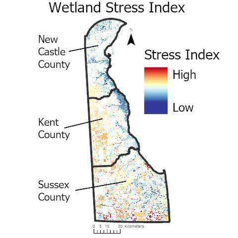
3.2. Rapidly Assessed Wetland Stress Index (RAWSI)

Much of Delaware’s naturally vegetated areas did not experience considerable loss during 2004–2018. However, as seen in Figure 3a, several areas, including areas within wetlands, experienced a decrease in NDVI. A total of 117 km² or 4.15% of naturally vegetated land experienced a decrease in NDVI from 2004 to 2018. However, most of these changes are not statistically significant (p > 0.05). Most areas that experienced a decrease in natural vegetation health over time were converted to either built land or crop fields by 2018. We found that approximately 1158 km of stream length (14.27%) is currently channelized within the study area. Our analysis indicates that 15.5% of areas within wetland buffers (150 m) are built land, while 35.4% are crop fields. The percentage of wetland areas experiencing natural vegetation loss is only 0.17%. Finally, 8.9% of stream lengths were identified as channelized within our defined wetland areas.

Throughout the entire State of Delaware, forested wetlands were shown to be experiencing the highest mean level of stress, followed by open water and non-forested wetlands. New Castle County, which is dominated by built land, contains the least number of wetlands, along with the least amount of stress occurring to wetlands overall (Figure 4). Kent County has a larger overall wetland area than New Castle and a higher overall amount of wetland stress (

Table 4. Wetland-specific distribution of the Rapidly Assessed Wetland Stress Index (RAWSI) with a minimum value (no stress) of 1 and maximum value of 100 (highest possible stress) over the counties and state.

Geographic Region	Wetland Type	Area (sq.km)	Mean RAWSI	Standard Deviation RAWSI
Delaware
	All Wetlands	1789.83	25.30	11.67
	Open Water	176.46	20.62	10.85
	Forested	1287.60	28.49	10.79
	Non-Forested	303.86	16.16	7.92
New Castle County
	All Wetlands	357.55	19.17	7.83
	Open Water	21.83	8.89	5.23
	Forested	267.03	22.03	6.45
	Non-Forested	68.69	11.32	4.70
Kent County
	All Wetlands	557.17	25.10	10.99
	Open Water	31.99	10.67	5.51
	Forested	388.31	30.59	7.93
	Non-Forested	136.87	12.89	4.83
Sussex County
	All Wetlands	872.50	27.98	12.39
	Open Water	121.92	25.41	9.09
	Forested	631.00	29.95	12.57
	Non-Forested	119.58	20.15	10.67

). This county also has the greatest number of non-forested wetlands that are shown to have a low mean level of stress. Sussex County is dominated by agriculture and also contains the largest extent of wetlands at 872.50 sq.km. The non-forested wetlands in this county also show a much higher level of stress when compared to non-forested wetlands in the other two counties. Mean stress for open water wetlands is also significantly higher when compared to other counties.

Our findings indicate significant spatial clustering within the RAWSI dataset, with a Global Moran’s I of 0.257 and p-value of <0.005. The Getis-Ord Gi* statistic indicated several significant clusters that can be seen in Figure 5. The clusters with high and low RAWSI values are referred to as hot spots and cold spots, respectively (Figure 5). Most non-forested wetlands are identified as cold spots, while many forested wetlands are identified as hot spots.

4. Discussion

The RAWSI data set, along with the independent stress indicators developed in this study, highlight many land-cover change trajectories in the state of Delaware, often at a regional scale. For example, the trend analysis for natural vegetation does not show statistically significant vegetation loss in most regions. However, landscape managers often need to focus on smaller regions (rather than the entire state) and must take into account notable changes in the region of interest, e.g., as seen in the Prime Hook National Wildlife Refuge (Figure 4b). This region lost considerable vegetation in 2006 due to a storm-induced flooding of two impoundments located on the refuge. Additionally, flooding from Hurricane Sandy in 2012 resulted in considerable habitat loss [90]. Such annual analyses are helpful in identifying the effects of recurring events.

In addition to extreme climatic events, ongoing hydrologic changes resulted in complete conversion in land-cover classes. Natural-vegetation loss was the biggest factor contributing to stress in coastal wetlands when compared to inland wetlands (Figure 4b). Approximately 11.24% of all vegetation loss since 2004 occurred within non-forested coastal wetlands, most likely due to the dynamic nature of coastal areas, resulting from tides, sea level changes, and storms. These hydrologic changes in coastal areas also led to the conversion of wetlands to open water (18.67%). These changes are represented in RAWSI through the NDVI loss analysis and represent wetland stress that occurred in the recent past. Considering annual land-cover maps, following methods presented here, and quantifying the change trajectory of each land-cover class can thus help the landscape managers in their direct planning efforts.

Delaware wetlands, and natural resources overall, are under considerable stress from anthropogenic activities, as well. Most inland vegetation loss in the state can be attributed to the conversion of forested areas to agricultural land (37.87%) or urban development (23%), between 2004 and 2018, predominately in Sussex County. However, the wetland stress is spatially distributed throughout the state, as indicated by the positive Global Moran’s I statistic (Figure 5). There is a striking difference between the spatial clustering—hot spots are mostly inlands, while cold spots are mostly coastal. This spatial differentiation is likely due to the laws protecting coastal wetlands in Delaware, as we see the land-cover stress being the largest factor impacting inland wetlands when compared to coastal wetlands (Figure 4a). Tidal wetlands are protected in Delaware, being subjected to either 50- or 100-foot landward buffer protections, thus restricting any development [91,92]. However, inland (nontidal) wetlands are only protected when they are larger than 400 acres, allowing for the conversion of these wetlands and their buffer areas. Higher amounts of stress were identified in Delaware’s lowermost county (Sussex), likely due to the dominance of agricultural land (Figure 5). Between counties, hydrology stress had the biggest impact. Sussex County also had a much higher level of hydrology stress compared to New Castle or Kent County, due to higher agricultural water use (Figure 4c). The abundance of agriculture may lead to increased stress through the channelization of streams (Figure 3b) to divert water for agricultural use.

The current literature shows that a combination of SAR and optical data results in improved accuracy of wetland classification [34,35,36,38,39,40]. Our study corroborates existing research for the forested wetland class when used with the RF classifier (Table 3). While per-class accuracy changed for the two sensor combinations used with the RF classifier, overall accuracies were comparable (Table 3). This comparison underscores the need to look beyond the overall accuracy and examine per-class accuracy for the classes of interest. While studies comparing RF and SVM show higher accuracy with SVM [65,66,67], our results consistently showed higher accuracy with RF. When choosing which classification method to use, a comparison of both RF and SVM on the training data may be beneficial. The high accuracy of our final wetland maps might be attributed to the simplified classification scheme of forested and non-forested wetlands. Unlike a few other studies [33,41,42,43], our classification scheme does not provide details on wetland classes, such as bog, fen, swamp, and marsh. However, the objective of our study was to accurately identify wetlands and existing stress factors, rather than identify more-detailed wetland classes.

Due to the inherent property of remote sensing as a tool, many aspects of DERAP/EPA rapid assessment procedures (such as detailed soil or plant characteristics) were not viable in this study. In the future, RAWSI can be further improved with advancements made in freely accessible high-resolution remotely sensed data, by incorporating those variables that were not considered in our study. We recommend the procedure presented in this study as a first step of a more detailed ground study. However, adopting RAWSI on an annual basis will considerably lower the cost of a timely update of wetland inventory, especially in rapidly transforming landscapes, due to ongoing natural and anthropogenic changes.

5. Conclusions

This study shows that a combination of optical and radar data when used with a Random Forest classifier might result in accurate land-cover maps, including wetland classes. This was shown with the combination of the Random Forest classifier with the radar data, which had a higher overall accuracy than the Support Vector Machine method or when radar data was not used. In this study we were able to assess metrics commonly attributed to wetland stress, including land cover, vegetation change, and stream channelization, through the use of remotely sensed and geographic data. All of these metrics were then combined into one Rapidly Assessed Wetland Stress Index (RAWSI), with each wetland area being assigned a stress value. Using a Getis-Ords Gi* statistic, we identified several hot spots of the RAWSI occurring within inland wetlands, especially in Kent and Sussex County in Delaware. Several cold spots of the RAWSI were also identified within coastal areas mostly contained in Kent County. The identification of hot and cold spots on a wetland-specific scale can be applied to understand spatial patterns of wetland stress, possibly giving insight into how current wetland regulations can be improved.

The informative new index RAWSI identified higher levels of stress among forested wetlands than non-forested wetlands and open water. The main factor contributing to higher stress in forested wetlands is land covers, such as urban and agriculture, within the wetland buffer. Even though non-forested wetlands experienced the lowest overall stress, the vegetation loss occurring within these wetlands provided higher amounts of stress than in any other wetland type. Higher stress is also observed in counties dominated by agriculture rather than urban areas. The channelization of streams was the biggest factor leading to higher stress in these agricultural regions. In the future, we recommend using any advancements in remote sensing to capture as many factors impacting a wetland as possible.

References

1. Environmental Protection Agency. What Is a Wetland? Environmental Protection Agency: Washington, DC, USA, 2018.
2. Cowardin, L.M. Classification of Wetlands and Deepwater Habitats of the United States; Fish and Wildlife Service: Washington, DC, USA, 1979.
3. Kennedy, V.; Greeson, P.E.; Clark, J.R.; Clark, J.E. Wetland Functions and Values: The State of Our Understanding. Estuaries 1981, 4, 388. [Google Scholar] [CrossRef]
4. Clarkson, B.R.; Ausseil, A.-G.E.; Gerbeaux, P. Wetland Ecosystem Services; Manaaki Whenua Press: Lincoln, New Zealand, 2014. [Google Scholar]
5. Dise, N.B. Peatland response to global change. Science 2009, 326, 810–811. [Google Scholar] [CrossRef] [PubMed]
6. Motts, W.; Heeley, R. A Guide to Important Characteristics and Values of Freshwater Wetlands in the Northeast. Water Resour. Res. Cent. 1973, 31, 5–8. [Google Scholar]
7. Odum, E. The Role of the Tidal Marshes in Estuarine Production; Conservationist: New York, NY, USA, 1961. [Google Scholar]
8. Brander, L.; Schuyt, K. Benefits Transfer: The Economic Value of World’s Wetlands; The Economics of Ecosystems Biodiversity: Geneva, Switzerland, 2004. [Google Scholar]
9. Tiner, R.W. Wetlands of the United States: Current Status and Recent Trends; Fish and Wildlife Service: Washington, DC, USA, 1984.
10. Winter, T.; Carr, M. Hydrologic Setting of Wetlands in the Cottonwood Lake Area, Stutsman County, North Dakota; US Geological Survey: Reston, VA, USA, 1980. [CrossRef]
11. Costanza, R.; D’Arge, R.; De Groot, R.; Farber, S.; Grasso, M.; Hannon, B.; Limburg, K.; Naeem, S.; O’Neill, R.V.; Paruelo, J.; et al. The value of the world’s ecosystem services and natural capital. Nature 1997, 387, 253–260. [Google Scholar] [CrossRef]
12. Mitsch, W.J.; Bernal, B.; Nahlik, A.M.; Mander, Ü.; Zhang, L.; Anderson, C.J.; Jørgensen, S.E.; Brix, H. Wetlands, carbon, and climate change. Landsc. Ecol. 2013, 28, 583–597. [Google Scholar] [CrossRef]
13. Davidson, N.C. How much wetland has the world lost? Long-term and recent trends in global wetland area. Mar. Freshw. Res. 2014, 65, 934–941. [Google Scholar] [CrossRef]
14. Winkler, M.G.; Dewitt, C.B. Environmental Impacts of Peat Mining in the United States: Documentation for Wetland Conservation. Environ. Conserv. 1985, 12, 317–330. [Google Scholar] [CrossRef]
15. Zedler, J.B.; Kercher, S. WETLAND RESOURCES: Status, Trends, Ecosystem Services, and Restorability. Annu. Rev. Environ. Resour. 2005, 30, 39–74. [Google Scholar] [CrossRef] [Green Version]
16. Tiner, R.; Biddle, M.; Jacobs, A.; Rogerson, A.; MucGukin, K. Delaware Wetlands: Status and Changes from 1992 to 2007; US Fish and Wildlife Service: Washington, DC, USA, 2011.
17. Tiner, R. Wetlands of Delaware; US Fish and Wildlife Service: Washington, DC, USA, 1985.
18. Sifneos, J.C.; Herlihy, A.T.; Jacobs, A.D.; Kentula, M.E. Calibration of the Delaware Rapid Assessment Protocol to a comprehensive measure of wetland condition. Wetlands 2010, 30, 1011–1022. [Google Scholar] [CrossRef]
19. Jacobs, A. Delaware Rapid Assessment Procedure Version 6.0 User’s Manual and Data Sheets; Delaware Department of Natural Resources and Environmental Control: Dover, DE, USA, 2010.
20. Fennessy, M.; Jacobs, A.; Kentula, M. Review of Rapid Methods for Assessing Wetland Condition; US Environmental Protection Agency: Washington, DC, USA, 2004.
21. Adam, E.; Mutanga, O.; Rugege, D. Multispectral and hyperspectral remote sensing for identification and mapping of wetland vegetation: A review. Wetl. Ecol. Manag. 2010, 18, 281–296. [Google Scholar] [CrossRef]
22. Guo, M.; Li, J.; Sheng, C.; Xu, J.; Wu, L. A review of wetland remote sensing. Sensors 2017, 17, 777. [Google Scholar] [CrossRef] [PubMed]
23. Ozesmi, S.L.; Bauer, M.E. Satellite remote sensing of wetlands. Wetl. Ecol. Manag. 2002, 10, 381–402. [Google Scholar] [CrossRef]
24. Tiner, R. Early Applications of Remote Sensing for Mapping Wetlands. In Remote Sensing of Wetlands: Applications and Advances; CRC Press: Boca Raton, FL, USA, 2015; pp. 67–78. [Google Scholar] [CrossRef]
25. Zomer, R.J.; Trabucco, A.; Ustin, S.L. Building spectral libraries for wetlands land cover classification and hyperspectral remote sensing. J. Environ. Manag. 2009, 90, 2170–2177. [Google Scholar] [CrossRef] [PubMed]
26. Gibbs, J.P. Wetland Loss and Biodiversity Conservation. Conserv. Biol. 2000, 14, 314–317. [Google Scholar] [CrossRef] [Green Version]
27. Delaware Firstmap 2019. Delaware 2007 Land Use, Land Cover. Available online: https://regional-delaware.opendata.arcgis.com/datasets/delaware-2007-land-use-land-cover (accessed on 20 August 2019).
28. Gilbertson, J.K.; Kemp, J.; van Niekerk, A. Effect of pan-sharpening multi-temporal Landsat 8 imagery for crop type differentiation using different classification techniques. Comput. Electron. Agric. 2017, 134, 151–159. [Google Scholar] [CrossRef] [Green Version]
29. Giri, C.; Pengra, B.; Long, J.; Loveland, T.R. Next generation of global land cover characterization, mapping, and monitoring. Int. J. Appl. Earth Obs. Geoinf. 2013, 25, 30–37. [Google Scholar] [CrossRef]
30. Jia, K.; Wei, X.; Gu, X.; Yao, Y.; Xie, X.; Li, B. Land cover classification using Landsat 8 Operational Land Imager data in Beijing, China. Geocarto Int. 2014, 29, 941–951. [Google Scholar] [CrossRef]
31. Peña, M.A.; Brenning, A. Assessing fruit-tree crop classification from Landsat-8 time series for the Maipo Valley, Chile. Remote Sens. Environ. 2015, 171, 234–244. [Google Scholar] [CrossRef]
32. Schultz, B.; Immitzer, M.; Formaggio, A.R.; Sanches, I.D.A.; Luiz, A.J.B.; Atzberger, C. Self-Guided segmentation and classification of multi-temporal Landsat 8 images for crop type mapping in Southeastern Brazil. Remote Sens. 2015, 7, 14482–14508. [Google Scholar] [CrossRef]
33. Banks, S.; White, L.; Behnamian, A.; Chen, Z.; Montpetit, B.; Brisco, B.; Pasher, J.; Duffe, J. Wetland Classification with Multi-Angle/Temporal SAR Using Random Forests. Remote Sens. 2019, 11, 670. [Google Scholar] [CrossRef]
34. Bourgeau-Chavez, L.; Endres, S.; Battaglia, M.; Miller, M.E.; Banda, E.; Laubach, Z.; Higman, P.; Chow-Fraser, P.; Marcaccio, J. Development of a Bi-National Great Lakes Coastal Wetland and Land Use Map Using Three-Season PALSAR and Landsat Imagery. Remote Sens. 2015, 7, 8655–8682. [Google Scholar] [CrossRef] [Green Version]
35. Dehouck, A.; Lafon, V.; Baghdadi, N.; Marieu, V. Use of optical and radar data in synergy for mapping intertidal flats and coastal salt-marshes (Arcachon lagoon, France). In Proceedings of the 2012 IEEE International Geoscience and Remote Sensing Symposium, Munich, Germany, 22–27 July 2012; pp. 2853–2856. [Google Scholar] [CrossRef]
36. Henderson, F.; Chasan, R.; Portolese, J.; Hart, T. Evaluation of SAR-Optical Imagery Synthesis Techniques in a Complex Coastal Ecosystem. Photogramm. Eng. Remote Sens. 2002, 68, 839–846. [Google Scholar]
37. Leckie, D.G. Synergism of synthetic aperture radar and visible/infrared data for forest type discrimination. Photogramm. Eng. Remote Sens. 1990, 56, 1237–1246. [Google Scholar]
38. Nsaibi, M.; Chaabane, F. Image fusion of radar and optical remote sensing data for land cover classification. In Proceedings of the 2008 3rd International Conference on Information and Communication Technologies: From Theory to Applications, ICTTA,, Damascus, Syria, 7–11 April 2008. [Google Scholar] [CrossRef]
39. Ramsey III, E.W.I.; Nelson, G.A.; Sapkota, S.K. Classifying coastal resources by integrating optical and radar imagery and color infrared photography. Mangroves Salt Marshes 1998, 2, 109–119. [Google Scholar] [CrossRef]
40. Ramsey III, E.; Rangoowala, A.; Tiner, R.; Klemas, V.; Lang, M. Radar and Optical Image Fusion and Mapping of Wetland Resources. In Remote Sensing of Wetlands: Applications and Advances; CRC Press: Boca Raton, FL, USA, 2015. [Google Scholar]
41. Salehi, B.; Mahdianpari, M.; Amani, M.; Manesh, F.; Granger, J.; Mahdavi, S.; Brisco, B. A Collection of Novel Algorithms for Wetland Classification with SAR and Optical Data. In Wetlands Management Assessing Risk and Sustainable Solutions; IntechOpen: Rijeka, Croatia, 2018. [Google Scholar] [CrossRef]
42. Touzi, R.; Deschamps, A.; Rother, G. Wetland characterization using polarimetric RADARSAT-2 capability. Can. J. Remote Sens. 2007, 33, S56–S67. [Google Scholar] [CrossRef]
43. Zhang, M.; Chen, F.; Tian, B.; Liang, D. Multi-temporal SAR image classification of coastal plain wetlands using a new feature selection method and random forests. Remote Sens. Lett. 2019, 10, 312–321. [Google Scholar] [CrossRef]
44. Gorelick, N.; Hancher, M.; Dixon, M.; Ilyushchenko, S.; Thau, D.; Moore, R. Google Earth Engine: Planetary-Scale geospatial analysis for everyone. Remote Sens. Environ. 2017, 202, 18–27. [Google Scholar] [CrossRef]
45. Shelestov, A.; Lavreniuk, M.; Kussul, N.; Novikov, A.; Skakun, S. Exploring Google earth engine platform for big data processing: Classification of multi-temporal satellite imagery for crop mapping. Front. Earth Sci. 2017, 5, 1–10. [Google Scholar] [CrossRef]
46. Chander, G.; Markham, B.L.; Helder, D.L. Summary of current radiometric calibration coefficients for Landsat MSS, TM, ETM+, and EO-1 ALI sensors. Remote Sens. Environ. 2009, 113, 893–903. [Google Scholar] [CrossRef]
47. Azzari, G.; Lobell, D.B. Landsat-Based classification in the cloud: An opportunity for a paradigm shift in land cover monitoring. Remote Sens. Environ. 2017, 202, 64–74. [Google Scholar] [CrossRef]
48. Hird, J.N.; DeLancey, E.R.; McDermid, G.J.; Kariyeva, J. Google earth engine, open-access satellite data, and machine learning in support of large-area probabilistic wetland mapping. Remote Sens. 2017, 9, 1315. [Google Scholar] [CrossRef]
49. Huang, H.; Chen, Y.; Clinton, N.; Wang, J.; Wang, X.; Liu, C.; Gong, P.; Yang, J.; Bai, Y.; Zheng, Y.; et al. Mapping major land cover dynamics in Beijing using all Landsat images in Google Earth Engine. Remote Sens. Environ. 2017, 202, 166–176. [Google Scholar] [CrossRef]
50. Mateo-García, G.; Gómez-Chova, L.; Amorós-López, J.; Muñoz-Marí, J.; Camps-Valls, G. Multitemporal cloud masking in the Google Earth Engine. Remote Sens. 2018, 10, 1079. [Google Scholar] [CrossRef]
51. Miettinen, J.; Shi, C.; Liew, S.C. Land cover distribution in the peatlands of Peninsular Malaysia, Sumatra and Borneo in 2015 with changes since 1990. Glob. Ecol. Conserv. 2016, 6, 67–78. [Google Scholar] [CrossRef] [Green Version]
52. Mondal, P.; Trzaska, S.; De Sherbinin, A. Landsat-Derived estimates of mangrove extents in the Sierra Leone coastal landscape complex during 1990–2016. Sensors 2018, 18, 12. [Google Scholar] [CrossRef] [PubMed]
53. Patela, N.N.; Angiuli, E.; Gamba, P.; Gaughan, A.; Lisini, G.; Stevens, F.R.; Tatem, A.J.; Trianni, G. Multitemporal settlement and population mapping from landsatusing google earth engine. Int. J. Appl. Earth Obs. Geoinf. 2015, 35, 199–208. [Google Scholar] [CrossRef]
54. Wingate, V.R.; Phinn, S.R.; Kuhn, N.; Bloemertz, L.; Dhanjal-Adams, K.L. Mapping decadal land cover changes in the woodlands of North Eastern Namibia from 1975 to 2014 using the landsat satellite archived data. Remote Sens. 2016, 8, 681. [Google Scholar] [CrossRef]
55. Xiong, J.; Thenkabail, P.S.; Tilton, J.C.; Gumma, M.K.; Teluguntla, P.; Oliphant, A.; Congalton, R.G.; Yadav, K.; Gorelick, N. Nominal 30-m cropland extent map of continental Africa by integrating pixel-based and object-based algorithms using Sentinel-2 and Landsat-8 data on google earth engine. Remote Sens. 2017, 9, 1065. [Google Scholar] [CrossRef]
56. ESA. Sentinel-1-SAR Technical Guide. Available online: https://sentinel.esa.int/web/sentinel/sentinel-technical-guides (accessed on 15 March 2019).
57. ESA. Sentinel-1: ESA’s Radar Observatory Mission for GMES Operational Services; European Space Agency: Paris, France, 2012. [Google Scholar]
58. White, L.; Brisco, B.; Dabboor, M.; Schmitt, A.; Pratt, A. A collection of SAR methodologies for monitoring wetlands. Remote Sens. 2015, 7, 7615–7645. [Google Scholar] [CrossRef]
59. Cutler, D.R.; Edwards, T.C.; Beard, K.H.; Cutler, A.; Hess, K.T.; Gibson, J.; Lawler, J.J. Random forests for classification in ecology. Ecology 2007, 88, 2783–2792. [Google Scholar] [CrossRef]
60. Prasad, A.M.; Iverson, L.R.; Liaw, A. Newer classification and regression tree techniques: Bagging and random forests for ecological prediction. Ecosystems 2006, 9, 181–199. [Google Scholar] [CrossRef]
61. Szuster, B.W.; Chen, Q.; Borger, M. A comparison of classification techniques to support land cover and land use analysis in tropical coastal zones. Appl. Geogr. 2011, 31, 525–532. [Google Scholar] [CrossRef]
62. Abe, B.T.; Olugbara, O.O.; Marwala, T. Experimental comparison of support vector machines with random forests for hyperspectral image land cover classification. J. Earth Syst. Sci. 2014, 123, 779–790. [Google Scholar] [CrossRef]
63. Noi, P.T.; Kappas, M. Comparison of random forest, k-nearest neighbor, and support vector machine classifiers for land cover classification using sentinel-2 imagery. Sensors 2018, 18, 18. [Google Scholar] [CrossRef]
64. Raczko, E.; Zagajewski, B. Comparison of support vector machine, random forest and neural network classifiers for tree species classification on airborne hyperspectral APEX images. Eur. J. Remote Sens. 2017, 50, 144–154. [Google Scholar] [CrossRef] [Green Version]
65. Breiman, L. Random Forests. Mach. Learn. 2001, 45, 5–32. [Google Scholar] [CrossRef] [Green Version]
66. Gong, P.; Wang, J.; Yu, L.; Zhao, Y.; Zhao, Y.; Liang, L.; Niu, Z.; Huang, X.; Fu, H.; Liu, S.; et al. Finer resolution observation and monitoring of global land cover: First mapping results with Landsat TM and ETM+ data. Int. J. Remote Sens. 2012, 34, 2607–2654. [Google Scholar] [CrossRef]
67. Huang, G.; Hongming, Z.; Xiaojian, D.; Rui, Z. Extreme Learning Machine for Regression and Multiclass Classification. Ieee Trans. Syst. Mancybern. Part B (Cybern.) 2011, 42, 513–529. [Google Scholar] [CrossRef]
68. Tony, Y. Understanding Random Forest. Available online: https://towardsdatascience.com/understanding-random-forest-58381e0602d2 (accessed on 1 August 2019).
69. Kulkarni, V.Y.; Sinha, P.K. Pruning of random forest classifiers: A survey and future directions. In Proceedings of the 2012 International Conference on Data Science and Engineering, ICDSE, Cochin, Kerala, India, 18–20 July 2012; pp. 64–68. [Google Scholar] [CrossRef]
70. Suykens, J.A.K.; Vandewalle, J. Least squares support vector machine classifiers. Neural Process. Lett. 1999, 9, 293–300. [Google Scholar] [CrossRef]
71. Kuemmerle, T.; Radeloff, V.C.; Perzanowski, K.; Hostert, P. Cross-Border comparison of land cover and landscape pattern in Eastern Europe using a hybrid classification technique. Remote Sens. Environ. 2006, 103, 449–464. [Google Scholar] [CrossRef]
72. Liu, W.; Gopal, S.; Woodcock, C.E. Uncertainty and confidence in land cover classification using a hybrid classifier approach. Photogramm. Eng. Remote Sens. 2004, 70, 963–971. [Google Scholar] [CrossRef]
73. Rozenstein, O.; Karnieli, A. Comparison of methods for land-use classification incorporating remote sensing and GIS inputs. Appl. Geogr. 2011, 31, 533–544. [Google Scholar] [CrossRef]
74. Oshiro, T.M.; Perez, P.S.; Baranauskas, J.A. How many trees in a random forest? In Proceedings of the International Conference on Machine Learning and Data Mining in Pattern Recognition, Berlin, Germany, 13–20 July 2012. [Google Scholar] [CrossRef]
75. Anderson, J.R.; Hardy, E.E.; Roach, J.T.; Witmer, R.E. A Land Use and Land Cover Classification System for Use with Remote Sensor Data; US Geological Survey: Reston, VA, USA, 1976.
76. Lillesand, T.; Kiefer, R.; Chipman, J. Remote Sensing and Image Interpretation. In Remote Sensing and Image Interpretation; John Wiley & Sons: Hoboken, NJ, USA, 2004; pp. 568–570. [Google Scholar]
77. Castelle, A.J.; Johnson, A.W.; Conolly, C. Wetland and Stream Buffer Size Requirements—A Review. J. Environ. Qual. 1994, 23, 878–882. [Google Scholar] [CrossRef]
78. Cohen, J. A Coefficient of Agreement for Nominal Scales. Educ. Psychol. Meas. 1960, 20, 37–46. [Google Scholar] [CrossRef]
79. Congalton, R.G. A review of assessing the accuracy of classifications of remotely sensed data. Remote Sens. Environ. 1991, 37, 35–46. [Google Scholar] [CrossRef]
80. Frank, E.; Hall, M.A.; Witten, I.H.; Kaufmann, M. WEKA Workbench Online Appendix for “Data Mining: Practical Machine Learning Tools and Techniques.”; Morgan Kaufmann: Burlington, MA, USA, 2016. [Google Scholar]
81. Pelleg, D.; Pelleg, D.; Moore, A. X-Means: Extending K-Means with Efficient Estimation of the Number of Clusters. In Proceedings of the 17th International Conference on Machine Learning, Stanford, CA, USA, 29 June–2 July 2000; pp. 727–734. [Google Scholar]
82. Gandhi, G.M.; Parthiban, S.; Thummalu, N.; Christy, A. Ndvi: Vegetation Change Detection Using Remote Sensing and Gis—A Case Study of Vellore District. Procedia Comput. Sci. 2015, 57, 1199–1210. [Google Scholar] [CrossRef]
83. Zhang, C.; Smith, M.; Lv, J.; Fang, C. Applying time series Landsat data for vegetation change analysis in the Florida Everglades Water Conservation Area 2A during 1996–2016. Int. J. Appl. Earth Obs. Geoinf. 2017, 57, 214–223. [Google Scholar] [CrossRef]
84. Simley, J. Applying the National Hydrography Dataset. J. Am. Water Resour. Assoc. 2008, 10, 5–8. [Google Scholar]
85. Savery, T.S.; Belt, G.H.; Higgins, D.A. Evaluation of the Rosgen Stream Classification System in Chequamegon-Nicolet National Forest, Wisconsin. J. Am. Water Resour. Assoc. 2001, 37, 641–654. [Google Scholar] [CrossRef]
86. Rosgen, D.L. A classification of natural rivers. Catena 1994, 22, 169–199. [Google Scholar] [CrossRef] [Green Version]
87. Mueller, J.E. An introduction to the hydraulic and topographic sinuosity indexes. Ann. Assoc. Am. Geogr. 1968, 58, 371–385. [Google Scholar] [CrossRef]
88. Goodchild, M. Spatial Autocorrelation; Geo Books: Norwich, UK, 1986. [Google Scholar]
89. Getis, A.; Ord, J.K. The Analysis of Spatial Association. Geogr. Anal. 1992, 24, 189–206. [Google Scholar] [CrossRef]
90. Guiteras, S. Prime Hook NWR Marsh Restoration—Early Evidence of Success. Available online: https://wmap.blogs.delaware.gov/2017/12/11/prime-hook-nwr-marsh-restoration-early-evidence-of-success/ (accessed on 20 August 2019).
91. Delaware Department of Natural Resources and Environmental Control. What is Regulated and Where is It Regulated? Delaware Department of Natural Resources and Environmental Control: Dover, DE, USA, 2019.
92. Environmental Law Institute. Delaware Wetland Program. Review; Environmental Law Institute: Washington, DC, USA, 2010. [Google Scholar]
Figure 1. The state of Delaware on the East Coast of the United States and a land-cover map from 2007 developed by Aerial Information Systems, along with county boundaries.
Remotesensing 11 02549 g001
Figure 2. Maps of the State of Delaware, showing (a) a false color composite (RGB = Near Infrared-Red-Green) of Landsat 8 images, showing median values for 2018 after cloud masking; (b) Sentinel-1 Synthetic Aperture Radar composite using three seasonal bands for spring, summer, and fall; and (c) the Random Forest supervised classification based on a combination of the Landsat 8 and Sentinel-1 datasets.
Remotesensing 11 02549 g002
Figure 3. Maps of the State of Delaware, showing (a) a decreasing trend in the normalized difference vegetation index (NDVI), an indicator of healthy vegetation, within naturally vegetated areas, such as forests and wetlands between 2004 and 2018; and (b) all streams, with non-channelized streams in blue with a sinuosity ratio greater than 1.06 and channelized streams in red with a sinuosity ratio less than or equal to 1.05.
Remotesensing 11 02549 g003
Figure 4. All wetland types mapped within the State of Delaware, showing (a) rescaled values for land-cover stressors, with high values denoting wetlands with either built or crop fields within an inclusive buffer of 150 m; (b) the amount of NDVI loss that each wetland area experienced from 2004 to 2018; (c) the length of channelized streams (sinuosity > 1.05) divided by the total length of streams within a wetland; (d) an overall Rapidly Assessed Wetland Stress Index (RAWSI), calculated by averaging the metrics from (ac). One value for all the metrics is assigned to each wetland polygon. The values for the three individual metrics (ac) were rescaled to 1–100 by the quantile that a certain value fell into when compared to the rest of the values within that metric. Maps are displayed with high stress values (100), symbolized in red, and low stress values (1), symbolized in blue.
Remotesensing 11 02549 g004
Figure 5. A statistical hot-spot analysis test (Getis-Ord Gi*) for the Rapidly Assessed Wetland Stress Index (RAWSI) values. Significant clusters of wetlands with a higher RAWSI values (hot spots) are shown in red, while significant clusters of lower RAWSI values (cold spots) are shown in blue. Nonsignificant clusters (p > 0.10) are shown in gray.
Remotesensing 11 02549 g005