Hyperspectral Anomaly Detection Based on Separability-Aware Sample Cascade

Abstract

A hyperspectral image usually covers a large scale of ground scene, which contains various materials with different spectral properties. When directly exploring the background information using all the image pixels, complex spectral interactions and inter-/intra-difference of different samples will significantly reduce the accuracy of background evaluation and further affect the detection performance. To address this problem, this paper proposes a novel hyperspectral anomaly detection method based on separability-aware sample cascade model. Through identifying separability of hyperspectral pixels, background samples are sifted out layer-by-layer according to their separable degrees from anomalies, which can ensure the accuracy and distinctiveness of background representation. First, as spatial structure is beneficial for recognizing target, a new spectral–spatial feature extraction technique is used in this work based on the PCA technique and edge-preserving filtering. Second, depending on different separability computed by sparse representation, samples are separated into different sets which can effectively and completely reflect various characteristics of background across all the cascade layers. Meanwhile, some potential abnormal targets are removed at each selection step to avoid their effects on subsequent layers. Finally, comprehensively taking different good properties of all the separability-aware layers into consideration, a simple multilayer anomaly detection strategy is adopted to obtain the final detection map. Extensive experimental results on five real-world hyperspectral images demonstrate our method’s superior performance. Compared with seven representative anomaly detection methods, our method improves the average detection accuracy with great advantages.

1. Introduction

A hyperspectral image is a data cube that simultaneously conveys rich spatial information and spectral information [1,2]. It can collect a wide range of electromagnetic spectrum nearly from visible to long-wavelength infrared. These spectra are represented by hundreds of continuous bands that can meticulously describe the characteristics of different materials to recognize their subtle differences [3]. Therefore, owing to this good discriminative property of hyperspectral image, it has been widely used in many remote sensing research fields [4,5], such as image denoising [6,7], hyperspectral unmixing [8,9], band selection [10,11], target detection [12,13], and image classification [14,15]. They all have important practical applications in geological exploration, urban remote sensing and planning management, environment and disaster monitoring, precision agriculture, archaeology, etc.

Due to its property of knowing nothing about the hyperspectral image scene, anomaly detection, as one special research problem of target detection, has attracted lots of attention in remote sensing field [16]. It aims at detecting the abnormal pixel whose spectrum has significant deviation from that of the given reference background. As it does not need any prior knowledge of both the target and the background, anomaly detection fits well with requirements of practical application because there is usually not a lot of information for unknown geographic scene. Consequently, it can be successfully used in a lot of practical applications [17,18,19,20], such as intelligent defense, food safety, medicine and health, forest fire protection, etc. Hyperspectral anomaly detection has played a crucial role in both military and civilian areas.

Over the past decades, a large number of anomaly detection methods for hyperspectral images have been proposed [21,22,23,24,25]. They can be roughly divided into two categories, i.e., distribution hypothesis-based methods and geometric model-based methods, which will be introduced in detail as follows. For the first category, the well-known Reed-Xiaoli (RX) [26] method is the most typical algorithm. It assumes that the background obeys the multivariate normal distribution. Therefore, Mahalanobis distance is adopted to compute the difference between one abnormal pixel and its surrounding background. Although RX is the most traditional method regarded as the benchmark, it still suffers from some important problems causing unsatisfactory detection performance when analyzing real-world images [27]. The small sample size is a tough problem of RX, which generates a badly conditioned matrix computation resulting in unstable results. In addition, unavoidable contamination of some potential abnormal targets embedding in the background will reduce the detection performance as well. Nevertheless, the intrinsic problem is the simple Gaussian distribution cannot accurately model the real hyperspectral image because of complex characteristics of the covered materials.

Many methods have been proposed aiming at improving the performance of RX through making some revisions to RX from different views. Instead of computing the covariance matrix using the reference background delineated by a local sliding window for local RX (LRX), the global RX (GRX) can directly use the whole image as background to evaluate its statistics. The regularized-RX (RRX) [28] method takes use of a scaled identity matrix to well adjust the property of estimated covariance matrix in order to address the effect of small sample size. There are also many methods that improve the performance through purifying background. For example, the random-selection-based anomaly detector (RSAD) [29] designs a sample random selection process to iteratively pick out some representative background pixels. Through carrying out this selection process for sufficient times, a better and purer background set can be obtained. The traditional blocked adaptive computationally efficient outlier nominator (BACON) [30] is also a robust method to the effects of anomalies. It starts from a basic subset that is affine equivariant and then continuously updates the basic set to construct the final basic subset to realize anomalies’ recognition. The kernel technique-based methods intend to improve the discrimination between background spectra and target information by mapping the original hyperspectral image into a feature space with high dimension. For example, kernel-RX (KRX) [31], a nonlinear version of RX, maps the linear non-Gaussian distribution data into nonlinear Gaussian that proves to be more accurate for anomaly detection. To improve the accuracy of background description, the cluster-based anomaly detector (CBAD) [32] is proposed, which adopts a clustering technique to segment the whole image into different clusters and, further, makes the hypothesis about each cluster obeying multivariate normal distribution. However, although these methods show their ability to improve the performance of RX, the intrinsic assumption still limits its performance.

As for the second category, geometric model-based methods commonly consider that there exist some representative spectra or dictionary bases to well characterize the background information. As one of the most important data representation types, sparse representation has been successfully applied in hyperspectral anomaly detection [33,34,35,36,37,38,39]. According to this philosophy, many methods have emerged in recent years. Yuan et al. [39] propose a local sparsity divergence method which simultaneously takes use of spectral and spatial divergence to analyze anomalies from the local reference background defined by a sliding window. Li et al. [36] propose constructing a collaborative representation-based detector (CRD), assuming that the background pixel can be approximately linearly represented by its surroundings, which is also a sparse representation-based detector (SRD). It further adopts a similarity matrix to regularize the collaborative representation in order to suppress the effects of anomalies. To obtain a more accurate description of background, a background joint sparse representation model [37] is designed to pick out the most active dictionary bases with the good ability to represent background. Taking sparse coefficient matrix having capabilities to reflect the atom usage frequency into consideration, a sparsity score estimation framework [40] is proposed to compute abnormal degree through combining the coefficient vector and atom usage probability. Ling et al. [41] propose a constrained sparse representation model which introduces both the sum-to-one and non-negativity constraints to satisfy physical meaning and simultaneously remove the constraint on the upper bound of sparsity level to avoid parameter setting. Taking advantage of the low rank property of background, Zhang et al. present a low-rank and sparse matrix decomposition-based Mahalanobis distance method (LSMAD) [38]. They impose the low-rank constraint on the background and the sparse constraint on anomalies in order to better decompose the background information from original hyperspectral images. Besides, there are also some manifold learning based methods which explore the data structure to detect anomalies. Olson et al. [42] construct a hyperspectral anomaly detection model in which the manifold learning technique is used to learn the background information. Yuan et al. [27] design a graph pixel selection process through combining the manifold learning technique and graph theory. The locally linear embedding (LLE) is used to discover the data structure that can contributes to the representation of anomalies.

In addition, some deep learning technique-based methods have been proposed in recent years. Using the advantages of deep learning architecture in data feature mining, researchers have explored its specific implementation in hyperspectral anomaly detection. There are two main ways: one is to fully learn the abstract representation of high-dimensional data from the perspective of unsupervised learning; the other is to use some label information or target information to guide the understanding of data characteristics from the perspective of supervised learning. Bati et al. propose an anomaly detection method based on autoencoder [43]. Through the coding–decoding process, background data can be decoded with a small reconstruction error, whereas the anomaly will have the larger reconstruction error. Zhao et al. use the stacked denoising autoencoders [44] to automatically learn the nonlinear deep features of hyperspectral images and achieve better detection results. Ma et al. design a detector based on a deep confidence network in which an adaptive weighting strategy is proposed to reduce the effect of local anomalies [45]. As for the supervised learning, it mainly uses external labeled hyperspectral images to guide the detection of anomalies in unknown scenes. Li et al. construct a transferred deep convolutional neural network to detect anomalies in the hyperspectral image [46]. Using the reference data with real labels, pixel pairs are generated to train the multi-layer CNN. For the pixel under test, its corresponding pixel pairs are obtained through computing the difference spectral vectors between it and all its surrounding pixels. Through statistically analyzing the similarity scores computed by the network, the final detection result can be obtained.

This work aims at addressing some challenges in the field of hyperspectral anomaly detection from the view of using traditional machine learning method. Although sparse representation based methods have proven its effectiveness in hyperspectral anomaly detection from the recently published literature [47], there are still some important problems that can have effects on the performance of anomaly detection. As we all know, real hyperspectral images commonly cover a vast geographical scene containing various materials with different spectral properties. Therefore, when directly exploring the background information using all the image pixels, an accurate background representation is hard to be learned because of the complex spectral interactions and inter-/intra-difference of different samples. Consequently, the detection performance will be reduced. Besides, potential anomalies embedding in the image scene can affect the background representation resulting in deterioration of performance as well. To address these problems, this paper proposes a novel hyperspectral anomaly detection based on separability-aware sample cascade, which tries to improve the description ability of background from the view of complex samples selection. Considering different pixels have different separable degrees from others, we can effectively divide them into different sample sets reflecting various material characteristics according to their separability. As a result, more accurate and complete background representation can be effectively obtained corresponding to each sample set belonging to different separation grades. Even though for the samples that are hard to be separated, the specially learned background information can also ensure the good ability to represent them. In our method, we gradually sift out all the samples layer-by-layer through the cascade structure in which sparse representation is used, to compute the separability of each sample. At the same time, we also remove potential anomalies from each layer in order to avoid feeding them into the next layer, which can ensure the good ability of background representation to resist the effects of anomalies. In addition, as spatial information is also important to recognize anomalies, we adopt a spectral–spatial feature extraction strategy to enhance the expressive ability. Note that our detection framework is applicable to different anomaly detectors, and the sparse representation is replaceable in this work. Main contributions of the proposed method can be summarized as follows.

(1)

Through identifying separability of hyperspectral pixels, a novel separability-aware sample cascade method is proposed to deeply and comprehensively explore the background characteristics. According to their separable degrees, it can effectively sift out all the pixel samples layer-by-layer, so that the learned background representation is more accurate and discriminative to express complex real hyperspectral image scenes.

(2)

Benefiting from automatically removing all the pixels with relatively lower separability in each cascade layer, it can directly avoid feeding the potential anomalies into the subsequent layers. Consequently, the proposed method can not only prepare purer data samples for sample selection of each layer, but also further ensure that the background characteristics have the good ability to restrain the effects of anomalies.

(3)

Taking both spectral and spatial information into consideration, a good spectral–spatial feature extraction strategy is used in this work. Through effectively combining the rich spectral properties naturally contained in the hyperspectral data and the structure properties obtained by using edge-preserving filter operation, we can extract features with higher expressive ability to characterize the deviation between target and background.

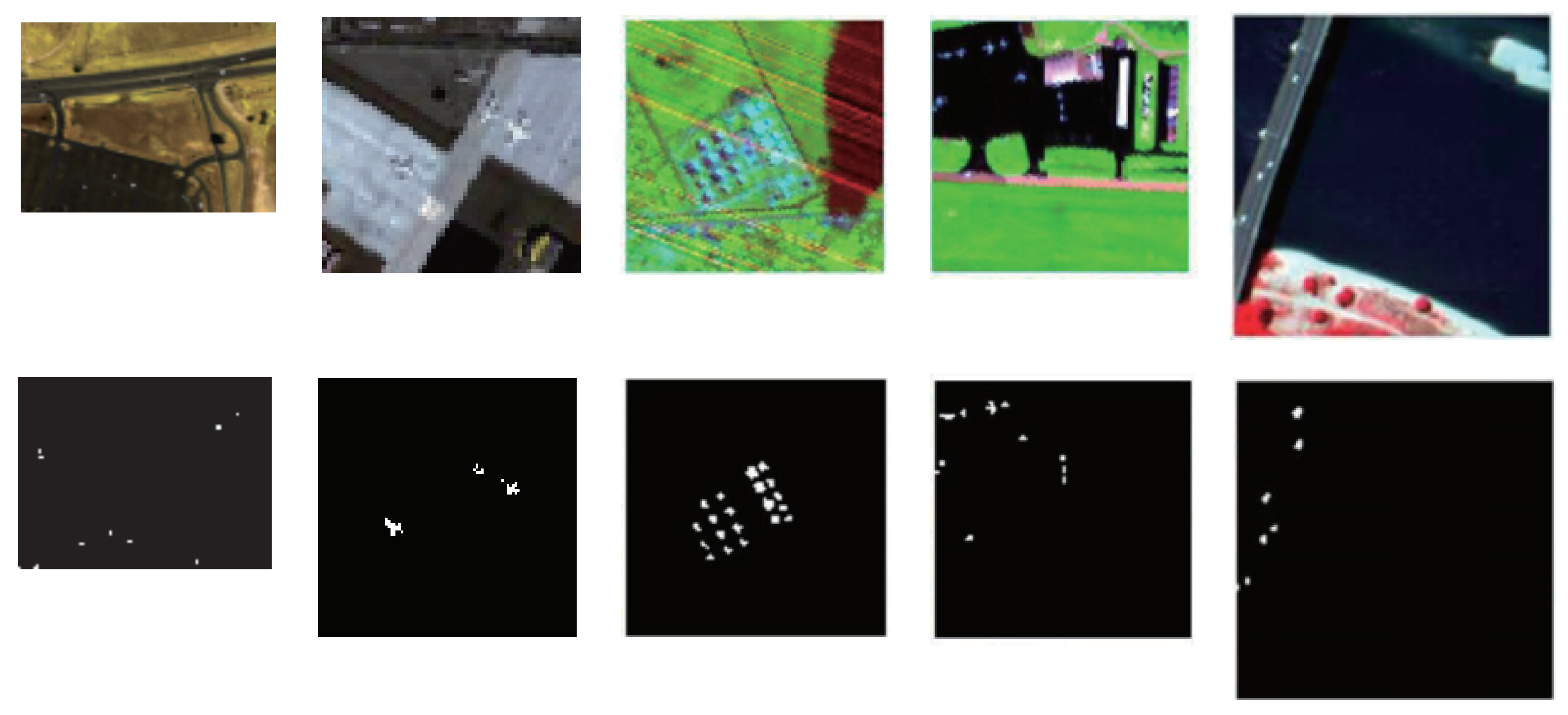
The rest parts of this paper are organized as follows. In Section 2, the proposed method is elaborated. In Section 3, experiments carried on five real hyperspectral images are introduced in detail. Finally, our work is summarized in Section 4.

2. Our Method

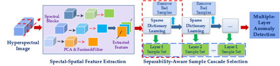
In this paper, we propose a novel anomaly detection method through constructing a separability-aware sample cascade model. As hyperspectral image pixels have complex spectral interactions and inter-/intra-difference, directly analyzing these samples as a whole to estimate background characteristics will result in unsatisfactory and inaccurate background evaluation. Consequently, anomaly detection will be further deeply affected. More precisely, when the analyzed pixels contain various kinds of materials or complicated interactions, precise background information presentation is really hard to be obtained. In fact, different pixels can be separated from others with different separability. If samples can be sifted out according to their different difficulties of separability, different background representation can be specifically obtained to make aware of samples with different deviations. In other words, for each kind of sample separated, from easily to difficultly separated, we can learn more accurate information to express samples’ characteristics. Our method contains three main procedures: (1) spectral–spatial feature extraction, (2) separability-aware sample cascade selection, and (3) multilayer anomaly detection.

First, we apply a new spectral–spatial feature extraction technique to take discriminative spectra and structure property into account at the same time. The traditional PCA and edge-preserving filtering are used in this operator, which can not only effectively remove redundant information, but also obtain useful spatial structure information to enhance expressive ability of each pixel sample. Secondly, we construct separability-aware sample cascade selection framework. Sparse representation is used to compute separability of each sample. According to their separable degrees, the relatively easily separated samples are sifted out and the bad samples with extremely low separability are simultaneously removed to delete their interference. Then the rest samples are fed into the next cascade layer to perform the same sample selection. Through passing all the samples layer-by-layer, we can obtain different sample sets with different separability-aware degrees from each cascade layer. Last, a multilayer anomaly detection strategy is presented to comprehensively take advantage of different separability-aware abilities of each layer in order to improve the detection performance. The proposed method will be elaborated in the following sections.

2.1. Spectral-Spatial Feature Extraction

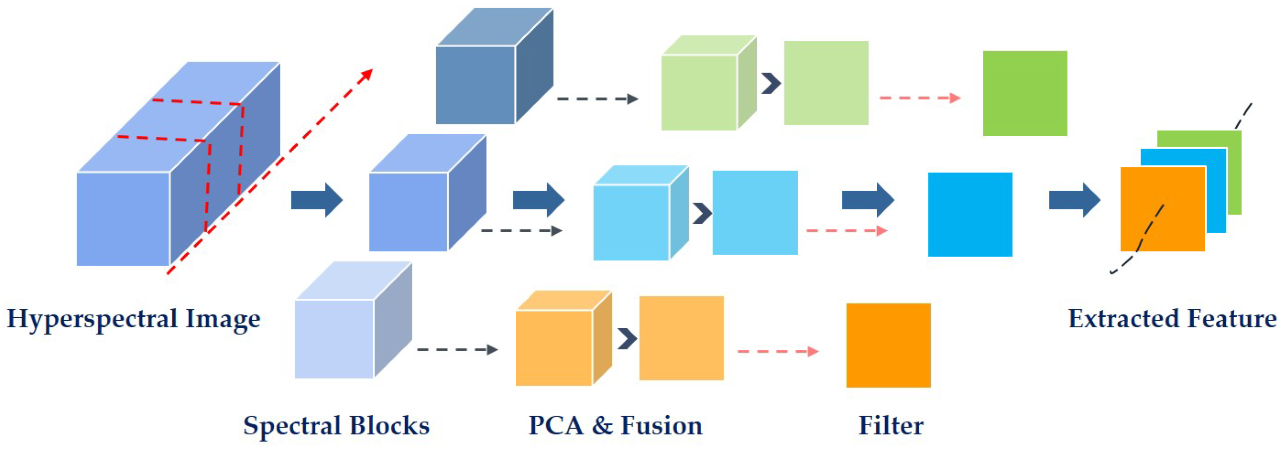
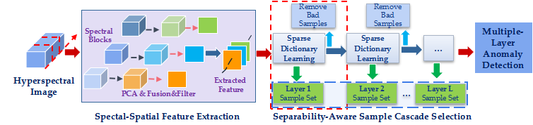
This part will introduce a new and simple spectral–spatial feature extraction technique. Figure 1 shows the flow chart of our feature extraction strategy. Through using this technique, the extracted feature can not only deliver rich spectral information, but also contain spatial structure information, which will have the stronger expressive ability to represent each data sample. At the same time, its low dimensional characteristic ensures the good performance in efficiency as well. Note that our used spectral–spatial feature extraction technique is inspired by that in [48], whose good performance has been demonstrated. Instead of directly using the technique proposed in [48], we embed the principal component analysis (PCA) strategy in it in order to eliminate the effects of some low signal–noise rate bands or unless bands.

As shown in Figure 1, we first divide the original hyperspectral cube into small blocks along the spectral dimension. Then for each block, PCA is used to explore the main pattern in data and remove noise as well. In order to take full use of different virtues of all the principal components, band fusion operation is carried out to completely combine all these principal bands together for further dimension reduction and information enhancement. After that, the edge-preserving filtering is carried out on each fused band to well preserve the spatial information. Finally, concatenating each fused band corresponding to each block together, a small new data cube with lower feature dimension is generated which delivers both the spectral and spatial information.

As our used spectral–spatial feature extraction technique is similar to the work [48]; therefore, we will briefly introduce it here following the flow chart shown in Figure 1. For a hyperspectral image cube $\mathbf{I}\in R^{H\times W\times B}$, H means the image height, W denotes the image width, and B is the number of spectral bands. Therefore, a single band image can be denoted as ${\mathbf{I}}^i\in R^{H\times W}(i=1,2,\dots ,B)$. When we divide $\mathbf{I}$ into K blocks along the spectral dimension, each block can be regarded as a set built with some adjacent band images. The index set of image bands contained in each blocks can be defined as follows,

$$D^k=\left\{\begin{array}{cc}\left\{\mathrm{f}\right(B/K)\times (k-1)+j|j\in \mathrm{I}+\wedge j\le \mathrm{f}(B/K)\},& if\\ \left\{\mathrm{f}\right(B/K)\times (K-1)+1,\mathrm{f}(B/K)\times (K-1)+2,\dots ,B\},& if\end{array}\begin{array}{c}k\in \{1,2,\dots ,K-1\}\\ k=K\end{array}\right.,$$

(1)

where $D^k$ is the index set for $k_{th}$ block, the $\mathrm{f}(B/K)$ function means that $B/K$ is rounded down to get the integer value, and $\mathrm{I}+$ is a set of positive integers. Therefore, each image block set ${\mathbf{B}}^k$ can be further obtained.

$$\begin{array}{cc}{\mathbf{B}}^k=\left\{{\mathbf{I}}^i\right|i\in D^k\},& k\in \{1,2,\dots ,K\}.\end{array}$$

(2)

Then, the PCA technique is carried out and m principal components are remained for each block. The fusion operation is further implemented on m principal components by using the traditional averaging strategy. Therefore, we can totally obtain K fused bands and the $k_{th}$ element can be denoted as ${\mathbf{I}}_{fused}^k\in R^{H\times W},k\in \{1,2,\dots ,K\}$. Then, according to the authors of [48,49], we carry out the edge-preserving filtering on each fused band. Therefore, our finally obtained small cube $\mathbf{H}\in R^{H\times W\times K}$ can be described as follows,

$${\mathbf{H}}^k={\mathrm{RF}}_{{\delta }_s,{\delta }_r}\left({\mathbf{I}}_{fused}^k\right),$$

(3)

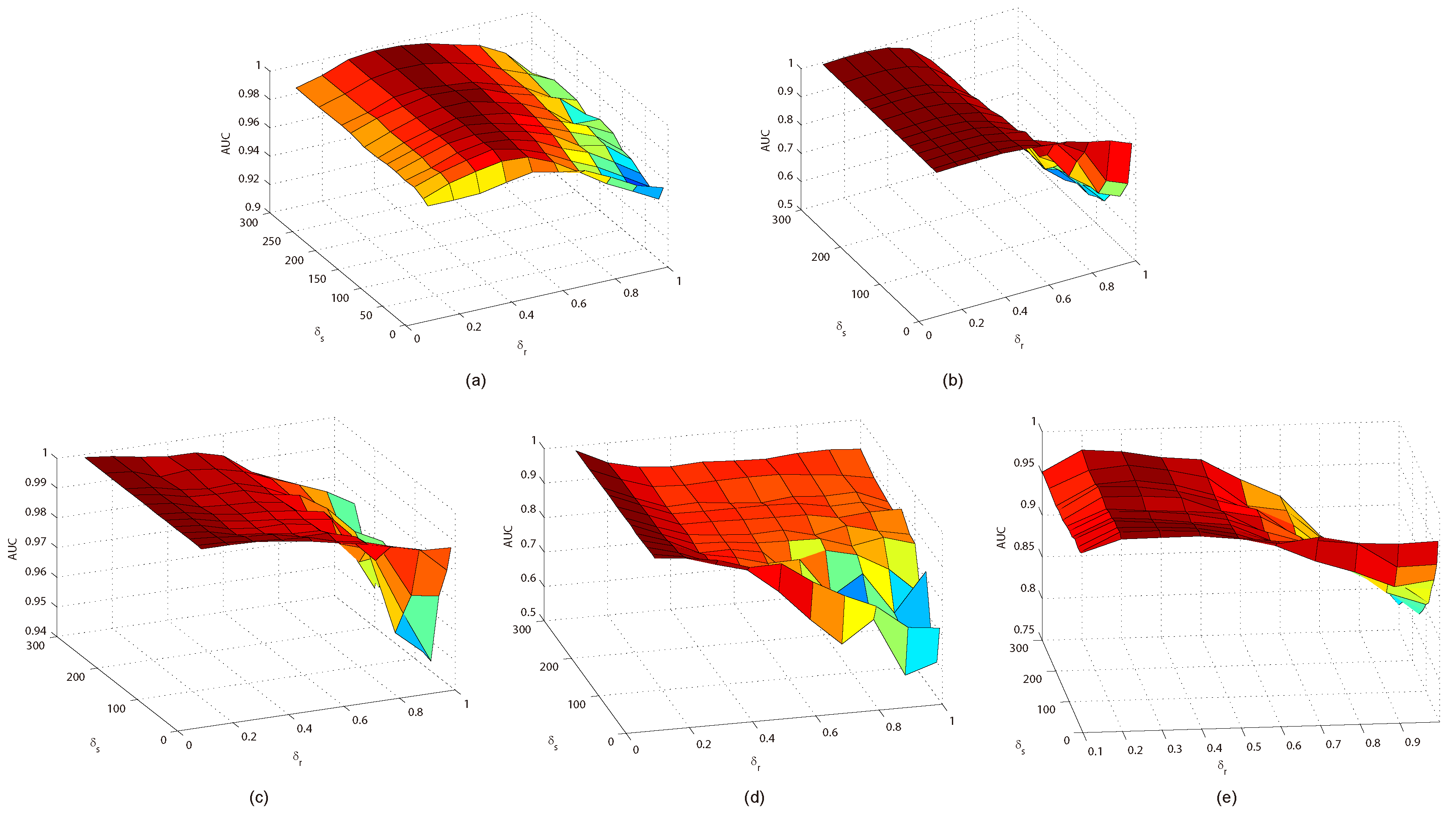
where ${\mathbf{H}}^k\in R^{H\times W},k=1,2,\dots ,K$ denotes the $k_{th}$ filtered band in the obtained cube data H. We adopt the same filter function ${\mathrm{RF}}_{{\delta }_s,{\delta }_r}(•)$, which is the transform domain recursive filter defined in [48]. Here, ${\delta }_s$ denotes the space standard deviation which mainly controls the blurring degree, and ${\delta }_r$ corresponds to the range, which mainly determines edge preservation. These two parameters can affect the effectiveness of the filter together.

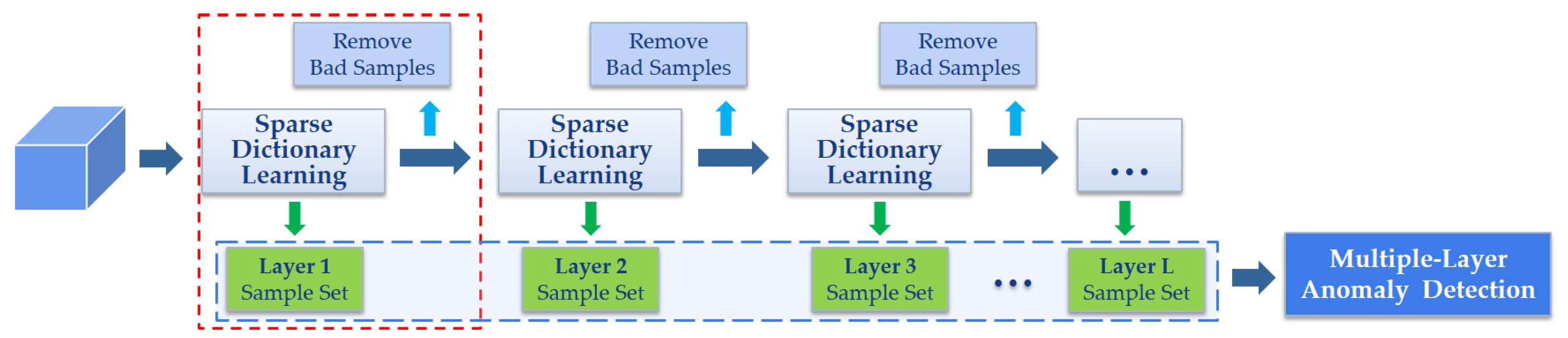
2.2. Separability-Aware Sample Cascade Selection

This part will introduce the separability-aware sample cascade selection process in detail. As sparse representation is commonly used in anomaly detection for its decent performance, our method is designed based on this representation model as well. However, due to the complex interference of various kinds of materials, accurate background representation will be affected. Therefore, we aim to address this problem through constructing a sample cascade selection on the basis of separability-aware idea. As per our proposed framework shown in Figure 2, different samples aware of different separable degrees can be effectively sifted out from the whole data set through the proposed sample cascade selection process. Meanwhile, we remove some potential targets as bad samples. Consequently, we can not only collect different sample sets with better representation ability specific to different background characteristics but also benefit from restraining the effects of some potential abnormal samples. The technical details will be introduced below.

For the small cube data $\mathbf{H}\in {}^{H\times W\times K}$ obtained by the above mentioned spectral–spatial feature extraction strategy, we reshape it into a 2D representation matrix $\mathbf{X}=\left[{\mathbf{x}}_1,{\mathbf{x}}_2,\dots ,{\mathbf{x}}_N\right]\in R^{K\times N}$, in which each row is generated by transforming each filtered band of $\mathbf{H}\in {}^{H\times W\times K}$ into a vector, respectively. Here, $N=H\times W$ is the total number of the cube data, and each column of $\mathbf{X}$, ${\mathbf{x}}_n\in R^K,n=1,2,\dots ,N$ denotes a pixel sample with K dimensions. Therefore, the traditional sparse representation model [50] can be formulated as

$$\underset{\mathbf{D},\mathbf{A},\parallel {\mathbf{d}}_{\mathbf{i}}\parallel \le \mathbf{1}}{min}{\parallel \mathbf{X}-\mathbf{DA}\parallel }_F^2+\lambda {\parallel \mathbf{A}\parallel }_1,$$

(4)

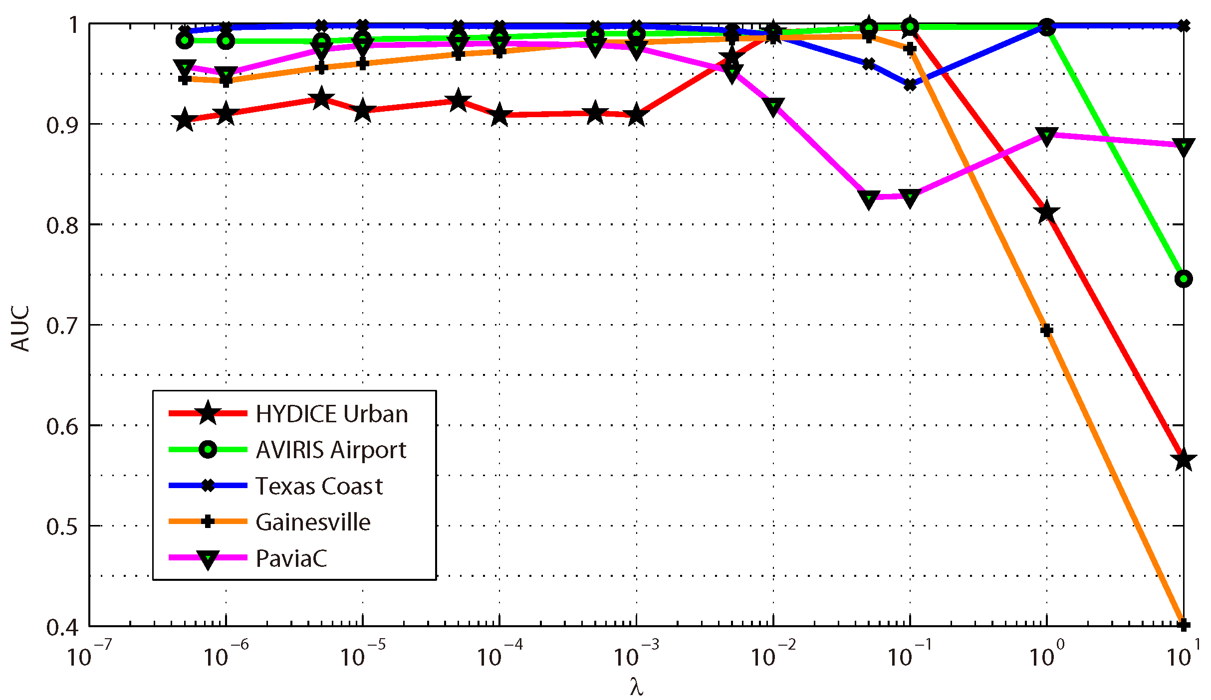
where $\mathbf{D}=\left[{\mathbf{d}}_1,{\mathbf{d}}_2,\dots ,{\mathbf{d}}_M\right]\in R^{K\times M}$ is the sparse representation dictionary containing M bases, $\mathbf{A}=\left[{\mathbf{a}}_1,{\mathbf{a}}_2,\dots ,{\mathbf{a}}_N\right]\in R^{M\times N}$ is the sparse coefficient matrix, and $\lambda$ is the regularization parameter. In this work, the dictionary learning technique proposed by Mairal et al. [51] is used to compute matrix $\mathbf{D}$. As for $\mathbf{A}$, when $\mathbf{D}$ is fixed, it turns to be the typical Lasso problem which can be easily solved. Therefore, the sparse reconstruction error $e_i$ for each sample can be computed as follows,

$$e_i={∥{\mathbf{x}}_i-\mathbf{D}{\mathbf{a}}_i∥}_2.$$

(5)

Therefore, reconstruction error vector for N input samples can be expressed as $\mathbf{e}={[e_1,e_2,\dots ,e_N]}^{\mathrm{T}}$. For simplicity, we directly regard the recovery value as the separability degree of each sample. The lower the reconstruction error is, the easier the sample is to be separated from others.

Then, we sift out the samples according to their separable degrees. First, the samples with relatively lower recovery errors will be picked out to build the separability-aware sample set for the current selection process. Second, the samples with relatively higher recovery errors which can be regarded as potential anomaly targets will be removed in order to reduce their effects on the next sample selection. The rest samples will be fed into the next layer to conduct the same selection process. By this way, we construct multiple layers connected in a cascade way to gradually separate all the pixels samples layer-by-layer according to different separability-aware degrees.

For better understanding, new mathematical symbols are introduced. As described above, the small cube data $\mathbf{X}$ is fed into the first layer to be sifted out. Consequently, it can be denoted as ${\mathbf{X}}_1=\left[{\mathbf{x}}_{{}_1}^1,{\mathbf{x}}_2^1,\dots ,{\mathbf{x}}_{N_1}^1\right]\in R^{K\times N_1}$, where $N_1=N$. The corresponding $\mathbf{e}$ can be expressed as ${\mathbf{e}}^1={[e_1^1,e_2^1,\dots ,e_{N_1}^1]}^{\mathrm{T}}$. Assuming that the input samples of the $l_{th}$ layer is ${\mathbf{X}}_l\in R^{K\times N_l},l=1,2,\dots ,L$, where $N_l$ is the total number of samples in current layer and L is the number of cascade layers in total; therefore, using Equations (4) and (5), we can learn the sparse dictionary, solve the coefficient matrix, and compute the reconstruction error vector ${\mathbf{e}}^l={[e_1^l,e_2^l,\dots ,e_{N_l}^l]}^{\mathrm{T}}$. Note that the matrix representation of the input samples can be simply regarded as a set whose elements correspond to the column vectors ${\mathbf{x}}_i^l$ in this work.

Then, we can sift out the separability-aware sample set ${\mathbf{B}}_l$ for the $l_{th}$ layer which can be written as

$${\mathbf{B}}_l=\left\{{\mathbf{x}}_i^l|e_i^l\le {\epsilon }_b\right\},$$

(6)

where ${\epsilon }_b$ is the separable threshold. Instead of fixing it at a constant, we use the value corresponding to the ${\eta }_b$ percentile of all the elements of current recovery error vector ${\mathbf{e}}^l$. Different ${\eta }_b$ will determine different ${\epsilon }_b$.

The removed sample set can be built as

$${\mathbf{R}}_l=\left\{{\mathbf{x}}_i^l|e_i^l>{\epsilon }_a\right\},$$

(7)

where ${\epsilon }_a$ is the removed threshold, which can be computed by the same way as ${\epsilon }_b$ through setting the ${\eta }_a$ percentile value. Therefore, we can finally obtain the rest samples which will be fed into the ${(l+1)}_{th}$ layer as its input data ${\mathbf{X}}_{l+1}$ by Equation (8).

$${\mathbf{X}}_{l+1}={\mathbf{X}}_l-{\mathbf{B}}_l-{\mathbf{R}}_l.$$

(8)

Removing the potential interference information is beneficial for learning background representation, because sample set ${\mathbf{X}}_{l+1}$ can be purified resulting in the following sample selection more accurate and robust. We will not terminate the same sample selection process until the stop condition is satisfied. In this work, we define the stop condition as

$$\mathrm{card}\left({\mathbf{X}}_l\right)<C.$$

(9)

The function $\mathrm{card}(•)$ is used to count the number of elements in a set. Therefore, this condition means that for a layer when the number of its input samples is less than a given constant C, the whole separability-aware sample cascade selection process will be stopped. At this time, if the last layer is the $L_{th}$ layer, there are totally L separability-aware sample sets ${\mathbf{B}}_l,l=1,2,\dots ,L$. Algorithm 1 summarizes the whole proposed selection process.

Algorithm 1 Separability-Aware Sample Cascade Selection

Input: Cube data sample set $\mathbf{X}\in R^{K\times N}$, regularized parameter $\lambda$, separable percentile ${\eta }_b$, removed percentile ${\eta }_a$, and constant C.

Output: All separability-aware sample sets ${\mathbf{B}}_l$.

1: Initialize $l=1$, ${\mathbf{X}}_l=\mathbf{X}$, $N_l=N$. 2: repeat 3:  Calculate the reconstruction errors ${\mathbf{e}}^l={[e_1^l,e_2^l,\dots ,e_{N_l}^l]}^{\mathrm{T}}$ by solving Equations (4) and (5). 4:  Calculate the separability-aware sample set ${\mathbf{B}}_l=\left\{{\mathbf{x}}_i^l|e_i^l\le {\epsilon }_b\right\}$. 5:  Calculate the removed sample set ${\mathbf{R}}_l=\left\{{\mathbf{x}}_i^l|e_i^l>{\epsilon }_a\right\}$. 6:  Calculate the input sample set for next layer ${\mathbf{X}}_{l+1}={\mathbf{X}}_l-{\mathbf{B}}_l-{\mathbf{R}}_l$. 7: until$\mathrm{card}\left({\mathbf{X}}_l\right)<C$.

2.3. Multiple-Layer Anomaly Detection

After finishing the separability-aware sample cascade selection process, totally L sample sets are generated from different layers. These sets have different separable degrees from each other. In other words, each sample set can characterize one specific property of the image scene. They can represent different discriminative abilities to perceive each sample’s deviation from the image scene. Therefore, we further present a multilayer anomaly detection strategy. Through comprehensively taking advantage of the different discriminative abilities of all these generated sample sets, the better detection performance can be achieved. Figure 2 also shows the multilayer anomaly detection strategy. Specifically, we feed each separability-aware sample set ${\mathbf{B}}_l$ as the dictionary into the traditional sparse representation model described by Equation (4), so the corresponding sparse matrix can be solved. Here, we denote each coefficient matrix as ${\mathbf{A}}_l$. Consequently, the joint detection results through fusing different decisions of all the layers can be computed as follows,

$$e_{mul}^i=\frac{{\displaystyle \sum _l}{∥{\mathbf{x}}_i-{\mathbf{B}}_l{\mathbf{a}}_i^l∥}_2}{L},$$

(10)

where ${\mathbf{x}}_i,i=1,2,\dots ,N$ is the $i_{th}$ sample of the input cube data, ${\mathbf{a}}_i^l$ is its corresponding sparse coefficient vector which is the $i_{th}$ column vector of matrix ${\mathbf{A}}_l$, and $e_{mul}^i$ is its final anomaly detection probability. Owing to the good virtue of multilayer anomaly detection strategy, we believe the proposed method has the better ability to detect various targets. No matter whether the target under test has higher separable degree or lower degree from the image scene, we can effectively recognize it by using the different discriminative abilities of different layers.

3. Experiments

In this paper, extensive experiments are conducted to demonstrate the effectiveness of the proposed method. Five different real-world hyperspectral images and seven representative anomaly detection methods are used to evaluate its performance in the experiments. In the following parts, we will respectively introduce the data sets, experimental set-up, experimental results, and parameter analysis in detail.

3.1. Data Sets

Five different available real-world hyperspectral images are tested in the experiments. These data sets cover various geographical scenes containing diverse materials and different types of abnormal targets. They can provide a convincing evaluation of an anomaly detection method. Figure 3 shows false color pictures and the corresponding ground truth maps of these images. For each ground truth map, anomalies are significantly highlighted, whereas the background is represented by the black area.

HYDICE urban image is the first data set. It is acquired by the HYDICE sensor from an aircraft through scanning an urban scene, which is provided by U.S. Army Engineer Research and Development Center. Its spectral range is 400 to 2500 nm with a total of 210 bands, leading to a spectral resolution of 10 nm. Referring to the work [27], fifty bands are usually removed in practice. There are $307\times 307$ pixels with a pixel size of about 2 m. When using this image for anomaly detection, researchers usually crop a sub-image with the size of $80\times 100$ from the original image because of the available ground truth map. It defines some cars and roofs as abnormal targets [40,50]. The first column of Figure 3 illustrates its visualization information.

The AVIRIS Airport image is the second data set. It is collected by the NASA’s Jet Propulsion Laboratory through the Airborne Visible/Infrared Imaging Spectrometer (AVIRIS) sensor on a airplane platform. This image covers the San Diego Airport, California, USA, containing some construction, vegetables, airstrips, and parking aprons. Its spectra range from 370 nm to 2510 with 224 bands in total. The spectral resolution is up to ~10 nm, and the spatial resolution is $3.5$ m. After removing several useless bands, 1–6, 33–35, 97, 107–113, 153–166, and 221–224, with relatively low signal–noise rates or water absorption regions, we keep 189 bands [52]. There are $100\times 100$ pixels in this subimage, and three planes are regarded as abnormal targets. The second column of Figure 3 shows its false-color image and ground truth map.

The Texas Coast hyperspectral image is the third data set. It is also acquired by the AVIRIS sensor, which can be downloaded from the website of AVIRIS (http://aviris.jpl.nasa.gov/). This image covers the urban scene near Texas coast. It has the spectral range of 370 nm to 2510 nm. After removing some noisy bands [53], totally 207 spectral channels are remained in the experiment. This image has the size of $100\times 100$. Its spatial resolution is ~17.2 m. A total of 20 targets with different kinds of sizes are defined as anomalies in this image scene. Its false color picture and the corresponding ground truth map are, respectively, illustrated in the third column of Figure 3.

The Gainesville image is the fourth data set. This image is same as the Texas Coast image for it is also collected by the AVIRIS sensor and can be downloaded from the same website. The difference is that this image has a higher spatial resolution of about $3.5$ m for it is acquired from a low-altitude aircraft through scanning the Gainesville urban scene. Considering the effects of some noisy bands, we keep 191 spectral bands, after removing 33 useless bands referring to the work [53]. There are $100\times 100$ pixels in the image, where totally 11 abnormal targets are located in. As shown in Figure 3, two rows of the fourth column show the related visualization information.

The PaviaC image scene is the fifth data set. It is provided by the Telecommunications and Remote Sensing Laboratory of Pavia University, which is collected by the ROSIS sensor on the airborne platform. It scans the scene near the central pavia in northern Italy, which mainly contains the bridge and water. The spectral range is from 430 to 860 nm with a total of 102 bands [38]. There are $150\times 150$ pixels with the geometric resolution of $1.3$ m. As for the definition of anomalies, some vehicles and small bare land areas are recognized as abnormal targets. Its false color picture and the corresponding ground truth map are respectively illustrated in the last column of Figure 3.

3.2. Experimental Details

In this part, we will elaborate the evaluation criterion, competitors, and parameter settings related to experiments as follows.

3.2.1. Evaluation Criterion

In the field of hyperspectral anomaly detection, the most commonly used evaluation criterion is the receiver operating characteristic (ROC) curve for qualitative analysis. It is drawn by a series of points. Each point is defined by a pair of values containing one true positive rate and one false alarm rate. Given one threshold, a pair of values will be computed according to detection results. This curve can accurately reflect the compromise between these two rates. As for the quantitative analysis, the AUC value (the area under the ROC curve), is usually used to compare the performance of different detectors. Concretely speaking, through carrying out the integral operator for ROC curve, the AUC value can be obtained. These two criteria are convincing and fair to evaluate the detection performance.

3.2.2. Competitors

In this paper, seven different state-of -the-art anomaly detection methods are used for complete comparison. The classical local RX (LRX), SRD, global RX (GRX), RSAD, BACON, LSMAD, and traditional sparse dictionary learning (DL) are chosen by comprehensively taking diversity, popularity, and timeliness into consideration. These methods are frequently adopted as competitors to evaluate the performance of a new anomaly detection method. Therefore, it is accurate and convincing to analyze the detection performance through comparing with these methods. Specially, LRX and GRX represent the typical Reed-Xiaoli method that is based on the statistical distribution hypothesis. SRD, LSMAD, and DL use sparse representation. As for RSAD and BACON, they are two popular methods that aim at obtaining pure background through reducing the effects of anomalies in order to improve the detection performance.

In addition, as the proposed method consists of two important stages, including the spectral–spatial feature extraction and the separability-aware sample cascade anomaly detection; therefore, we also conduct the ablation study experiment to analyze the effectiveness of these two stages. As sparse dictionary learning is the basic detection model for the proposed method, we successively compare with the DL method in the ablation study experiment. For simplicity, when we only use the spectral–spatial feature extraction strategy and then carry out the traditional DL detection method, we denote this case as Ours-DL-S; when both spectral–spatial feature extraction strategies and separability-aware sample cascade anomaly detection, in other words, the whole proposed procedures, are completely carried out, we denote this case as Ours-DL-SS. Actually, Ours-DL-SS represents our method.

3.2.3. Parameter Settings

Some main parameters involved in the experiments are declared in this section. First, the parameter settings of our proposed method are introduced in detail. For the stage of spectral–spatial feature extraction, there are three critical parameters: the number of divided blocks K, the space standard deviation ${\delta }_s$, and the range standard deviation ${\delta }_r$. The value of K determines the dimension of finally generated new feature. The filter parameters ${\delta }_s$ and ${\delta }_r$ affect the performance of filtering. As for the stage of separability-aware sample cascade anomaly detection, three important parameters, i.e., the regularization parameter $\lambda$, the separable percentile ${\eta }_b$, and the removed percentile ${\eta }_a$, will be elaborated. ${\eta }_b$ can determine the scale of each separability-aware sample set that will have effects on the number of cascade layers. ${\eta }_a$ can directly decide the size of the removed samples which in fact aims at getting rid of the potential anomalies. Therefore, as a matter of experience that anomalies usually have a small population with low occurrence probability, ${\eta }_a$ is empirically fixed at $99.5$ percentile. As the effects of parameters K, ${\delta }_s$, ${\delta }_r$, $\lambda$, and ${\eta }_b$ on the detection performance seem relatively complex, we further conduct the corresponding parameter selection experiments in order to deeply analyze and discuss their properties in Section 3.4.

Here, we just declare the final settings of these parameters involved in the following comparison experiment. For the five hyperspectral images, K is completely fixed at 20, ${\delta }_s$ is set as 100, $0.2$ is assigned to ${\delta }_r$; the values of $\lambda$ are $0.05$, $0.05$, ${10}^{-5}$, $0.005$, and ${10}^{-4}$ in turn; and ${\eta }_b$ is fixed at 10. In addition, except for the above principal parameters, there are also some simple parameters needed to be claimed for a clearer and better understanding of our method. The number of principal components of PCA during the feature extraction process is set as 3. The number of bases is defined as the twice K for each sparse dictionary. As for the constant C in the stop condition, its value is also set as the twice K. In other words, when the number of rest samples is less than the size of dictionary, the sample cascade selection process will be stopped. Note that the parameters of DL, Ours-DL-S, and Ours-DL-SS keep consistent with each other in the experiments.

As for competitors, their parameter settings are introduced as well. As LRX and SRD use the dual windows [54] to detect local anomalies, two kinds of window sizes consisting of the outside window and the inner window (outside and inner) should be defined. Therefore, considering that such detectors adopting a sliding window strategy are usually sensitive to the window sizes, different pairs of window sizes are set in order to convincingly reflect their detection performance. Taking account of both characteristics of different hyperspectral images and requirements of different detectors’ parameter settings, we define four pairs of window sizes for LRX—$(17,7)$, $(17,9)$, $(19,7)$, and $(19,9)$—and six pairs of window sizes for SRD—$(13,7)$, $(15,9)$, $(17,7)$, $(17,9)$, $(19,7)$, and $(19,9)$. Besides, we set the optimal value for the regularized parameter of SRD for each hyperspectral image in the experiment. As for RSAD, the size of image block is set as 70 during the random selection process. The value of parameter c involved in BACON is fixed at 4 referring to the original literature [30]. As for LSMAD, the optimal parameters on each image have been selected. The values of matrix’s maximal rank r are 2, 1, 2, 5, and 2, and the values of sparse cardinality k are set as $0.7$, $0.3$, $0.005$, $0.6$, and $0.4$ for the five hyperspectral images, respectively.

3.3. Comparison Results

In this part, extensive experimental results will be completely and deeply analyzed in order to fairly and convincingly evaluate the performance of our proposed method. The visualization results of all the methods on five hyperspectral images are respectively illustrated in Figure 4, Figure 5, Figure 6, Figure 7 and Figure 8, whereas the corresponding ROC curves are shown in Figure 9.

Table 1. Area under the ROC curve (AUC) values for quantitive analysis of all the competitors’ performance on five real-world hyperspectral images. The optimal values of window sizes are underlined. The highest AUC values are highlighted by the bold numbers.

AUC		HYDICE Urban	AVIRIS Airport	Texas Coast	Gainesville	PaviaC
LRX	(17,7)	0.8467	0.7352	0.8758	0.7581	0.9418
	(17,9)	0.8242	0.7264	0.8311	0.7472	0.9338
	(19,7)	0.9095	0.8361	0.8598	0.8143	0.9383
	(19,9)	0.8862	0.8585	0.8454	0.7999	0.9352
SRD	(13,7)	0.9456	0.9102	0.8885	0.7317	0.9524
	(15,7)	0.9475	0.9163	0.8878	0.7089	0.9449
	(17,7)	0.9438	0.9231	0.8967	0.7021	0.9462
	(17,9)	0.9395	0.9342	0.8776	0.7282	0.9385
	(19,7)	0.9459	0.9171	0.8933	0.7003	0.9467
	(19,9)	0.9423	0.9329	0.8818	0.7152	0.9378
GRX		0.8906	0.9611	0.9946	0.9513	0.9538
RSAD		0.8781	0.9437	0.8091	0.9390	0.6739
BACON		0.6861	0.7271	0.7205	0.6362	0.8574
LSMAD		0.9598	0.9801	0.9048	0.9279	0.9218
DL		0.8398	0.8189	0.8687	0.8519	0.8253
Ours-DL-S		0.9165	0.9904	0.9474	0.9575	0.9299
Ours-DL-SS		0.9965	0.9953	0.9983	0.9848	0.9808

presents AUC values, and

Table 2. Average AUC of each competitor using all data sets and average performance improvement of our method to each competitor.

Methods	LRX	SRD	GRX	RSAD	BACON	LSMAD	DL	Ours-DL-S	Ours-DL-SS
AUC	0.8800	0.8925	0.9503	0.8488	0.7255	0.9389	0.8409	0.9483	0.9911
Improvement	11.11%	9.86%	4.08%	14.23%	26.56%	5.22%	15.02%	4.28%	-

shows the average AUC values of all the data sets for each detector and our corresponding improvement to other competitors. Note that all the results of LRX and SRD on different window sizes are shown in Table 1, and their best results for each hyperspectral image are underlined. The visualization pictures and ROC curves corresponding to their optimal window sizes are just shown in this paper for convenience of layout.

Figure 4 illustrates the visualization pictures of all the detection methods on HYDICE Urban data set. It can be seen that RSAD and BACON made many obvious mistakes that recognize the background area as abnormal targets. LRX cannot seem to effectively locate the targets for there are many omissions. The result of DL presents much background clutter. SRD, GRX, LSMAD, Ours-DL-S, and Ours-DL-SS show better detection performance, because anomalies can be clearly recognized from their visualization results. Moreover, Ours-DL-SS outperforms the other four methods for it can not only assign high intensities to anomalies but also effectively suppress the background clutter. The ROC curve shown in Figure 9a demonstrates this conclusion as well. The ROC curve of our proposed method (denoted as Ours-DL-SS) is almost significantly above all the other methods’ curves. It always obtains a higher detection rate for a given false alarm rate among all the ROC curves. Our method can achieve promising detection performance, even though the false positive rate is less than ${10}^{-3}$, which fully proves its good distinctiveness. As for the quantitative analysis, the highest AUC value shown in Table 1 demonstrates the excellent detection performance again. Therefore, it can be concluded that our proposed method has superior ability to be aware of the difference between the target and the background.

Figure 5 illustrates the visualization pictures of all the detection methods on AVIRIS Airport hyperspectral image. Similarly, BACON has a serious problem of high false alarm rate. As for RSAD, it can significantly detect all the anomalies with less background detection mistakes. LRX seems to completely miss all the abnormal targets. The result is hard to estimate for SRD from its visualization map. DL also contains lots of background clutter. As for GRX, LSMAD, Ours-DL-S, and Ours-DL-SS, they show the similar detection results for all the targets have been effectively detected. The most difference is that anomalies are highlighted with different intensities by them. Compared with the other three methods, Ours-DL-SS is better for its detected targets are much more notable while the background is well suppressed. To carry out a fair and convincing evaluation of the detection performance, we further analyze ROC curves and AUC values on this image. From Figure 9b, it can be seen that Our-DL-SS defeats all the other methods except for LSMAD, because its ROC curve lies above their ROC curves. Comparing with LSMAD, when the false positive rate takes the smaller value, the detection rate of our method is slightly lower than that of LSMAD, but when the false positive rate takes a larger value, our ROC curve will keep above LSMAD. From the results shown in Table 1, we can see that our method obtains the highest AUC value. On the whole, all the results have demonstrated the good performance of the proposed method. It has good distinctiveness to recognize anomalies from the real scene.

Figure 6 illustrates the visualization pictures of all the detection methods on Texas Coast image. Both RSAD and BAON have serious false alarm rates. LRX, SRD, and DL seem to miss the targets. As for LSMAD, although it can detect some anomalies, it has a problem of false alarm rate as well. GRX, Our-DL-S, and Our-DL-SS show better performance for they can detect more targets. Moreover, compared with the other three, the targets detected by our method are more salient. The ROC curves shown in Figure 9c further verify the superior performance of the proposed method. Our ROC curve has absolute advantage for it is far higher than other curves. Our method shows good detection ability, even though the alarm rate is very low. It also obtains the highest AUC value as shown in Table 1. According to all these comparison, the effectiveness of the proposed method has been demonstrated. Our method benefits the good virtue of subtly perceiving the discrepancy between targets and background through separability-aware sample cascade selection process.

Figure 7 illustrates the visualization pictures of all the detection methods on Gainesville image. BACON still faces an obvious problem of high false alarm rate. RSAD also suffers from some background detection mistakes. SRD can locate a few targets but with lots of background clutters. LRX and DL cannot clearly locate anomalies. As for GRX, LSMAD, Ours-DL-S, and Ours-DL-SS, they show better results that are similar to each other from the view of visualization. Figure 9d shows the ROC curves of all the methods on this data set. Our curve also achieves the best performance for it nearly outperforms all the other curves along all the value range of false positive rate. At the same time, our method also achieves the highest AUC value that is far ahead of those of most other methods. All these results convincingly verify that out method has the good distinctiveness to recognize different targets from the background. Through separating all the hyperspectral pixels into different sample sets, better background representation can be obtained specific to different material properties.

Figure 8 illustrates the visualization pictures of all the detection methods on PaviaC image. As for BACON and RSAD, their results’ analyses are similar to their corresponding results on the previous data. SRD, DL, and Ours-DL-S have obvious background clutter. LRX, GRX, and LSMAD have similar results, and they can detect some targets. As for the proposed method, it shows better result for it completely recognizes all the targets and simultaneously assigns salient intensities to them. The highest ROC curve shown in Figure 9e fully verifies the effectiveness of our method. It always stays above all the other curves, which shows its good detection ability. Our method also obtains the optimal AUC value which is really a promising result. Owing to sifting out samples according to their separability, the background information can be deeply and accurately discovered, and the deviation of anomalies from background can be significantly enlarged. Consequently, our method can successfully distinguish different kinds of anomalies.

The above parts mainly carry out the comparison with other representative competitors. So as to deeply analyze the effectiveness of different stages of our proposed method, we further discuss the ablation study experiment. Through completely analyzing both qualitative results shown in Figure 9 and quantitive values illustrated in Table 1, some reasonable conclusions can be drawn. First, the performance of traditional DL belongs to lower middle level of detection ability among all the methods. Second, the performance of Ours-DL-S is obviously better than that of DL, which robustly demonstrates the effectiveness of our spectral–spatial feature extraction strategy. Nevertheless, Ours-DL-S just improves the performance to the level slightly above moderate of detection ability for it is still inferior to many state-of-the-art methods. At last, Ours-DL-SS is significantly better than Ours-DL-S which convincingly verifies the excellent performance of separability-aware sample cascade anomaly detection process. Ours-DL-SS successfully raises the detection performance to the highest level. According to all these analyses, each stage of our proposed method has demonstrated its effectiveness.

On the whole, based on all the comparison and analyses, the proposed method outperforms all the representative detectors. It not only has the good ability to recognize different kinds of targets from various real-world scenes, but also shows its superiority in suppressing the background. The highest average AUC value of all the results on five hyperspectral images achieved by our method also objectively verifies its robust and excellent detection performance as shown in Table 2. Compared with seven representative anomaly detection methods, our method improves the average detection accuracy by approximately $11.11\%$, $9.86\%$, $4.08\%$, $14.23\%$, $26.56\%$, $5.22\%$, and $15.02\%$, respectively. Owing to the spectral–spatial extraction strategy, the generated features have more expressive ability to recognize the deviation of targets from background. Through further separating various and complex materials into different samples and simultaneously removing some potential targets, accurate and complete background characteristics resisting to anomalies’ effects can be fully explored, which forcefully ensures the good performance of our method.

3.4. Parameters Setting Discussion

In this section, the effects of crucial parameters involved in the proposed method are analyzed and discussed in detail. We further explore the setting criteria or selection suggestions for them. The experiments are mainly conducted on the five mentioned parameters consisting of the number of divided blocks K, the space standard deviation ${\delta }_s$, the range standard deviation ${\delta }_r$, the regularization parameter $\lambda$, and separable percentile ${\eta }_b$. To completely and objectively explore their effects on detection performance, experiments are carried out on all the five hyperspectral images.

The number of divided blocks K deciding the dimension of extracted feature is chosen from the set of $\left\{3,5,10,15,20,25,30,35,40,50\right\}$ in sequence. Figure 10 presents the experimental result. It can be seen that the curves’ trends of all the data sets are nearly similar. When K is equal to 3, although their AUC are slightly lower, they are still satisfactory results. Then all the curves rapidly move up to promising performance and nearly maintain the higher AUC values. On the whole, our method has good robustness to different number of divided blocks. Therefore, we finally fix it at 20 for all the data sets for simplicity.

As for the filtering parameters ${\delta }_s$ and ${\delta }_r$, their effects are jointly analyzed. The space standard deviation ${\delta }_s$ is chosen from the set of $\left\{10,20,40,60,80,100,120,150,180,200,250,300\right\}$. The range standard deviation ${\delta }_r$ changes from $0.1$ to 1 at the interval of $0.1$. The experiments are illustrated in Figure 11. Taking all the results of all the hyperspectral images into consideration, our method is almost not sensitive to these two parameters. The detection performance stably changes within a promising range in most cases. Specifically, for all the real-world images, when ${\delta }_r$ is approximately less than $0.6$, all the AUC values are good and nearly unchanged, which fully demonstrates the effectiveness of our method. Consequently, we set ${\delta }_s$ as 100 and ${\delta }_r$ as 0.2 for all the hyperspectral images.

Then, the effects of regularization parameter $\lambda$ is analyzed. Totally, 14 different values build the set $\left\{5\times {10}^{-7},{10}^{-6},5\times {10}^{-6},{10}^{-5},5\times {10}^{-5},{10}^{-4},5\times {10}^{-4},{10}^{-3},5\times {10}^{-3},{10}^{-2},5\times {10}^{-2},{10}^{-1},{10}^0,{10}^1\right\}$ to be chosen for $\lambda$. Comparing all the curves shown in Figure 12, on the whole, these five curves have similar slopes in despite of some small difference in local areas. When $\lambda \le {10}^{-3}$, all the curves achieve good detection results, and each of them stably and gently changes within slight floating. When $\lambda$ continues to increase, both curves of AVIRIS Airport and Gainesville still gradually move up initially, and then they begin to go down from different values, whereas the curve of HYDICE Urban has a relatively obvious rise at the very beginning, and then its trend changes like the curve of Gainesville; however, curves of Texas Coast and PaviaC are a little different because they first decrease, and then increase again to become stabilized. Comprehensively considering all the results, although the optimal values of $\lambda$ for each images are different, when $\lambda$ is equal to or lesser than 1, our detection performance on all the different data sets is decent, which becomes better and more stable especially in the range of equal to or lesser than ${10}^{-3}$. In the experiments, for each hyperspectral image, $\lambda$ takes the corresponding optimal value. Specifically, the values of $\lambda$ are set as $0.05$, $0.05$, ${10}^{-5}$, $0.005$, and ${10}^{-4}$ for HYDICE Urban, AVIRIS Airport, Texas Coast, Gainesville, and PaviaC, respectively.

As for separable percentile ${\eta }_b$, its values change from 5 to 40 at the interval of 5. The corresponding results are plotted in Figure 13. It can be clearly seen that our method also has good robustness to this parameter for all the curves are either nearly unchanged or just have slight changes within the higher AUC value range. Moreover, all the results corresponding to all different values of ${\eta }_b$ are excellent for they are larger than $0.97$, which strongly verifies the good performance of our method. For convenience, ${\eta }_b$ is fixed at 10 in the comparison experiment.

4. Conclusions

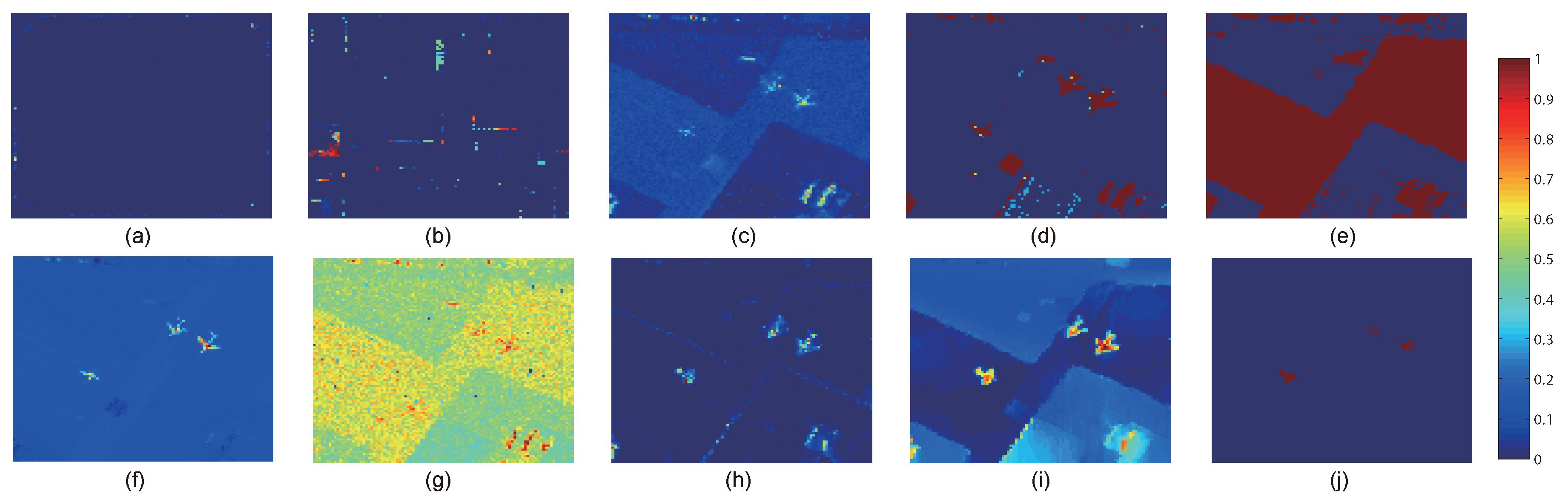
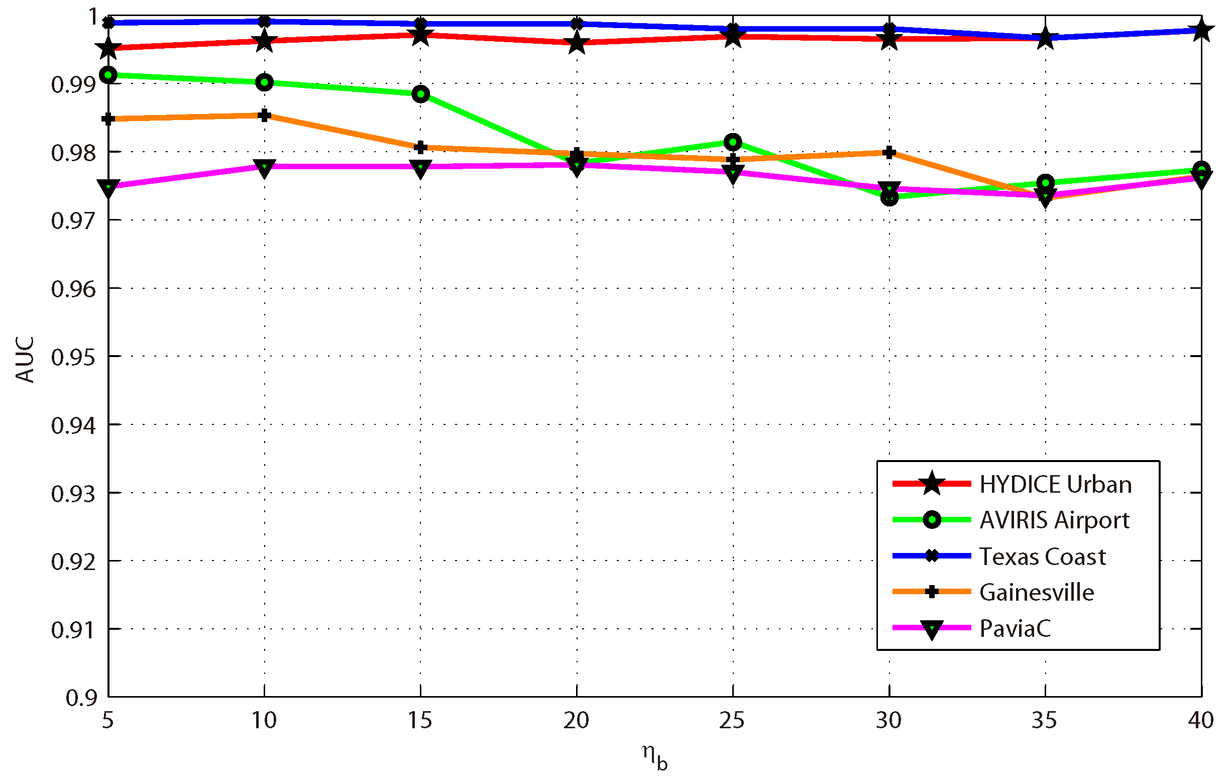
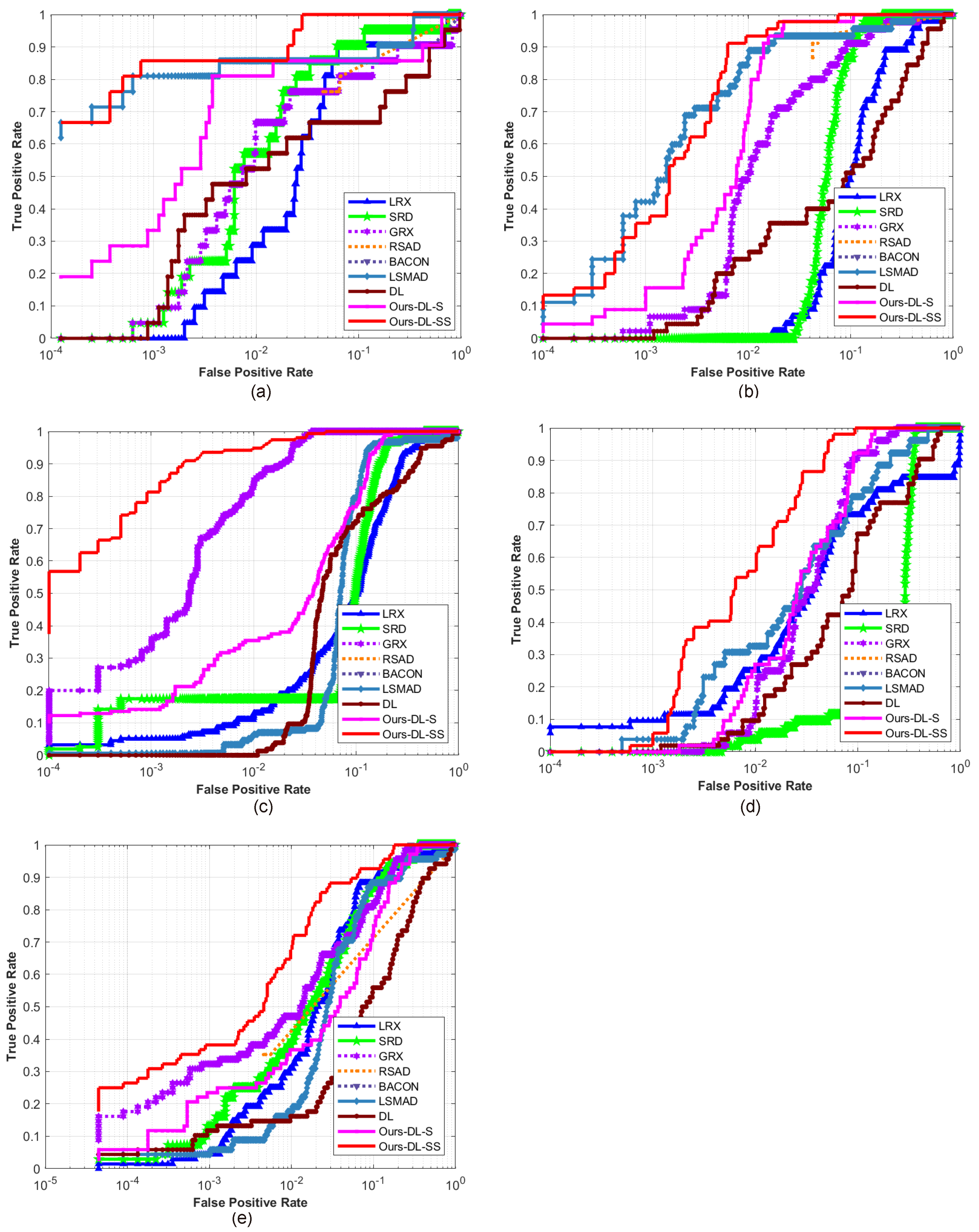
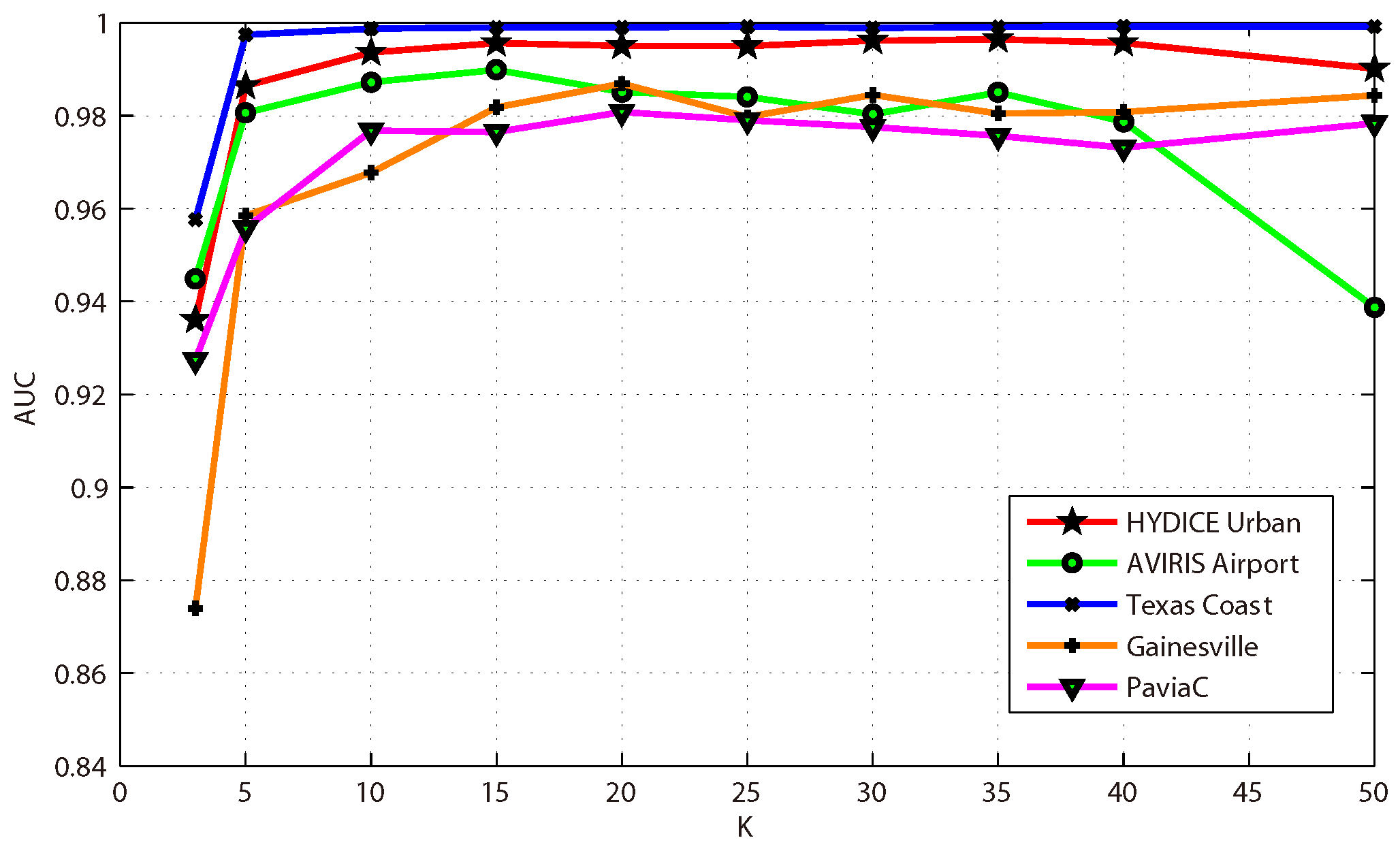
This paper presents an effective anomaly detection method for hyperspectral images through designing a separability-aware sample cascade model. It aims at addressing the unsatisfactory detection performance caused by the inaccurate scene information representation because of complex spectral interactions and inter-/intra-difference of different samples. Through sifting out all the hyperspectral pixel samples according to their different separable degrees, more accurate and complete background information can be explored specific to different separated sample sets with various material characteristics. The proposed method mainly consists of three important procedures including spectral–spatial feature extraction, separability-aware sample cascade selection, and multilayer anomaly detection. Taking use of spectral–spatial feature extraction, both spectral information and spatial structure information can be obtained which can enhance the expressive ability to recognize targets. Then, we construct the separability-aware sample cascade selection framework, which can divide samples into different sets layer-by-layer and simultaneously removes the potential abnormal targets at each selection step. Consequently, our learned background representation can not only have good distinctiveness to recognize different anomalies from real images scenes, but also benefits from the good ability to restrain effects of potential anomalies. Finally, we simply adopt the multilayer anomaly detection strategy in order to comprehensively take different good characteristics of all the separability-aware layers into consideration. In the experiments, our proposed method is compared with seven state-of-the-art detectors on five different real-world hyperspectral images to fairly and convincingly evaluate its performance. Extensive experimental results demonstrate the effectiveness of our method. It has achieved superior performance to all these representative competitors. Specifically, compared with LRX, SRD, GRX, RSAD, BACON, LSMAD, and DL, our method has obvious performance improvement of about $11.11\%$, $9.86\%$, $4.08\%$, $14.23\%$, $26.56\%$, $5.22\%$, and $15.02\%$, respectively, in accordance with their average AUC values of all the hyperspectral images. Besides, through deeply analyzing and discussing the sufficient parameter setting experiment, our method also has good robustness to different parameters. On the whole, the proposed method has good performance to detect different abnormal targets from various hyperspectral scenes covering different materials, which outperforms all the employed state-of-the-art competitors.

References

1. Zhu, L.; Wen, G. Hyperspectral anomaly detection via background estimation and adaptive weighted sparse representation. Remote Sens. 2018, 10, 272. [Google Scholar]
2. Yuan, Y.; Ma, D.; Wang, Q. Hyperspectral anomaly detection via sparse dictionary learning method of capped norm. IEEE Access. 2019, 7, 16132–16144. [Google Scholar] [CrossRef]
3. Zhao, L.; Lin, W.; Wang, Y.; Li, X. Recursive local summation of rx detection for hyperspectral image using sliding windows. Remote Sens. 2018, 10, 103. [Google Scholar] [CrossRef]
4. Wang, Q.; Lin, J.; Yuan, Y. Salient band selection for hyperspectral image classification via manifold ranking. IEEE Trans. Neural Netw. Learn. Syst. 2016, 27, 1279–1289. [Google Scholar] [CrossRef]
5. Wang, Q.; Qin, Z.; Nie, F.; Li, X. Spectral embedded adaptive neighbors clustering. IEEE Trans. Neural Netw. Learn. Syst. 2017, 30, 1265–1271. [Google Scholar] [CrossRef]
6. Rasti, B.; Scheunders, P.; Ghamisi, P.; Licciardi, G.; Chanussot, J. Noise reduction in hyperspectral imagery: Overview and application. Remote Sens. 2018, 10, 482. [Google Scholar] [CrossRef]
7. Gao, L.; Yao, D.; Li, Q.; Zhuang, L.; Zhang, B.; Bioucas-Dias, J. A new low-rank representation based hyperspectral image denoising method for mineral mapping. Remote Sens. 2017, 9, 1145. [Google Scholar] [CrossRef]
8. Zhang, X.; Li, C.; Zhang, J.; Chen, Q.; Feng, J.; Jiao, L.; Zhou, H. Hyperspectral unmixing via low-rank representation with space consistency constraint and spectral library pruning. Remote Sens. 2018, 10, 339. [Google Scholar] [CrossRef]
9. Rizkinia, M.; Okuda, M. Joint local abundance sparse unmixing for hyperspectral images. Remote Sens. 2017, 12, 1224. [Google Scholar] [CrossRef]
10. Liu, K.; Chen, S.; Chien, H.; Lu, M. Progressive sample processing of band selection for hyperspectral image transmission. Remote Sens. 2018, 10, 367. [Google Scholar] [CrossRef]
11. Yuan, Y.; Lin, J.; Wang, Q. Dual-clustering-based hyperspectral band selection by contextual analysis. IEEE Trans. Geosci. Remote Sens. 2016, 54, 1431–1445. [Google Scholar] [CrossRef]
12. Alarcon-Ramirez, A.; Rwebangira, M.; Chouikha, M.; Manian, V. A new methodology based on level sets for target detection in hyperspectral images. IEEE Trans. Geosci. Remote Sens. 2016, 54, 5385–5396. [Google Scholar] [CrossRef]
13. Zhang, Y.; Wu, K.; Du, B.; Zhang, L.; Hu, X. Hyperspectral target detection via adaptive joint sparse representation and multi-task learning with locality information. Remote Sens. 2017, 9, 482. [Google Scholar] [CrossRef]
14. He, Z.; Wang, Y.; Hu, J. Joint sparse and low-rank multitask learning with laplacian-like regularization for hyperspectral classification. Remote Sens. 2018, 10, 322. [Google Scholar] [CrossRef]
15. Gao, L.; Zhao, B.; Jia, X.; Liao, W.; Zhang, B. Optimized kernel minimum noise fraction transformation for hyperspectral image classification. Remote Sens. 2017, 9, 548. [Google Scholar] [CrossRef]
16. Nasrabadi, N. Hyperspectral target detection: An overview of current and future challenges. IEEE Signal Process. Mag. 2014, 31, 34–44. [Google Scholar] [CrossRef]
17. Wang, Q.; Gao, J.; Li, X. Weakly supervised adversarial domain adaptation for semantic segmentation in urban scenes. IEEE Trans. Image Process. 2019, 28, 4376–4386. [Google Scholar] [CrossRef]
18. Wang, Q.; Wan, J.; Li, X. Robust hierarchical deep learning for vehicular management. IEEE Trans. Veh. Technol. 2018. [Google Scholar] [CrossRef]
19. Wang, Q.; Chen, M.; Nie, F.; Li, X. Detecting coherent groups in crowd scenes by multiview clustering. IEEE Trans. Pattern Anal. Machine Intell. 2018. [Google Scholar] [CrossRef]
20. Wang, Q.; Wan, J.; Nie, F.; Liu, B.; Yan, C.; Li, X. Hierarchical feature selection for random projection. IEEE Trans. Neural Netw. Learn. Syst. 2019, 30, 1581–1586. [Google Scholar] [CrossRef]
21. Matteoli, S.; Acito, N.; Diani, M.; Corsini, G. An automatic approach to adaptive local background estimation and suppression in hyperspectral target detection. IEEE Trans. Geosci. Remote Sens. 2011, 49, 790–800. [Google Scholar] [CrossRef]
22. Kwon, H.; Nasrabadi, N.M. Kernel matched subspace detectors for hyperspectral target detection. IEEE Trans. Pattern Anal. Mach. Intell. 2006, 28, 178–194. [Google Scholar] [CrossRef] [PubMed]
23. Khazai, S.; Safari, A.; Mojaradi, B.; Homayouni, S. An approach for subpixel anomaly detection in hyperspectral images. IEEE J. Sel. Top. Appl. Earth Obs. Remote Sens. 2013, 6, 769–778. [Google Scholar] [CrossRef]
24. Matteoli, S.; Diani, M.; Corsini, G. A tutorial overview of anomaly detection in hyperspectral images. IEEE Trans. Aerosp. Electron. Syst. 2010, 25, 5–28. [Google Scholar] [CrossRef]
25. Sun, W.; Tian, L.; Xu, Y.; Du, B.; Du, Q. A randomized subspace learning based anomaly detector for hyperspectral imagery. Remote Sens. 2018, 10, 417. [Google Scholar] [CrossRef]
26. Reed, I.; Yu, X. Adaptive multiple-band CFAR detection of an optical pattern with unknown spectral distribution. IEEE Trans. Acoust. Speech Sign. Proc. 1990, 38, 1760–1770. [Google Scholar] [CrossRef]
27. Yuan, Y.; Ma, D.; Wang, Q. Hyperspectral anomaly detection by graph pixel selection. IEEE Trans. Cybern. 2016, 46, 3123–3134. [Google Scholar] [CrossRef]
28. Nasrabadi, N. Regularization for spectral matched filter and RX anomaly detector. Proc. SPIE 2008, 6966, 696604-1–696604-12. [Google Scholar]
29. Du, B.; Zhang, L. Random-selection-based anomaly detector for hyperspectral imagery. IEEE Trans. Geosci. Remote Sens. 2011, 49, 1578–1589. [Google Scholar] [CrossRef]
30. Billora, N.; Hadib, A.; Velleman, P. BACON: Blocked adaptive computationally efficient outlier nominators. Comput. Stat. Data Anal. 2000, 34, 279–298. [Google Scholar] [CrossRef]
31. Kwon, H.; Nasrabadi, N.M. Kernel rx-algorithm: A nonlinear anomaly detector for hyperspectral imagery. IEEE Trans. Geosci. Remote Sens. 2005, 43, 388–397. [Google Scholar] [CrossRef]
32. Carlotto, M.J. A cluster-based approach for detecting man-made objects and changes in imagery. IEEE Trans. Geosci. Remote Sens. 2005, 43, 374–387. [Google Scholar] [CrossRef]
33. Xu, Y.; Wu, Z.; Li, J.; Plaza, A.; Wei, Z. Anomaly detection in hyperspectral images based on low-rank and sparse representation. IEEE Trans. Geosci. Remote Sens. 2016, 54, 1990–2000. [Google Scholar] [CrossRef]
34. Niu, Y.; Wang, B. Hyperspectral anomaly detection based on low-rank representation and learned dictionary. Remote Sens. 2016, 8, 289. [Google Scholar] [CrossRef]
35. Zhang, Y.; Du, B.; Zhang, L.; Liu, T. Joint sparse representation and multitask learning for hyperspectral target detection. IEEE Trans. Geosci. Remote Sens. 2017, 55, 894–906. [Google Scholar] [CrossRef]
36. Li, W.; Du, Q. Collaborative representation for hyperspectral anomaly detection. IEEE Trans. Geosci. Remote Sens. 2015, 53, 1463–1474. [Google Scholar] [CrossRef]
37. Li, J.; Zhang, H.; Ma, L. Hyperspectral anomaly detection by the use of background joint sparse representation. IEEE J. Sel. Top. Appl. Earth Obs. Remote Sens. 2015, 8, 2523–2533. [Google Scholar] [CrossRef]
38. Zhang, Y.; Du, B.; Zhang, L.; Wang, S. A low-rank and sparse matrix decomposition-based Mahalanobis distance method for hyperspectral anomaly detection. IEEE Trans. Geosci. Remote Sens. 2016, 54, 1376–1389. [Google Scholar] [CrossRef]
39. Yuan, Z.; Sun, H.; Ji, K.; Li, Z.; Zou, H. Local sparsity divergence for hyperspectral anomaly detection. IEEE Geosci. Remote Sens. Lett. 2014, 11, 1697–1701. [Google Scholar] [CrossRef]
40. Zhao, R.; Du, B.; Zhang, L. Hyperspectral anomaly detection via a sparsity score estimation framework. IEEE Trans. Geosci. Remote Sens. 2017, 55, 3208–3222. [Google Scholar] [CrossRef]
41. Ling, Q.; Guo, Y.; Lin, Z.; An, W. A constrained sparse representation model for hyperspectral anomaly detection. IEEE Trans. Geosci. Remote Sens. 2018, 57, 2358–2371. [Google Scholar] [CrossRef]
42. Olson, C.; Coyle, M.; Doster, T. A study of anomaly detection performance as a function of relative spectral abundances for graph- and statistics-based detection algorithms. Proc. SPIE 2017. [Google Scholar] [CrossRef]
43. Bati, E.; Çalışkan, A.; Koz, A.; Alatan, A. Hyperspectral anomaly detection method based on autoencoder. Proc. SPIE 2015, 9643, 220–226. [Google Scholar]
44. Zhao, C.; Li, X.; Zhu, H. Hyperspectral anomaly detection based on stacked denoising autoencoders. J. Appl. Remote Sens. 2017, 11, 042605. [Google Scholar] [CrossRef]
45. Ma, N.; Peng, Y.; Wang, S.; Phw, L. An unsupervised deep hyperspectral anomaly detector. Sensors. 2018, 18, 693. [Google Scholar] [CrossRef] [PubMed]
46. Li, W.; Wu, G.; Du, Q. Transferred deep learning for anomaly detection in hyperspectral imagery. IEEE Geosci. Remote Sens. Lett. 2017, 14, 597–601. [Google Scholar] [CrossRef]
47. Ma, D.; Yuan, Y.; Wang, Q. Hyperspectral anomaly detection via discriminative feature learning with multiple-dictionary sparse representation. Remote Sens. 2018, 10, 745. [Google Scholar] [CrossRef]
48. Kang, X.; Li, S.; Benediktsson, J. Feature extraction of hyperspectral images with image fusion and recursive filtering. IEEE Trans. Geosci. Remote Sens. 2014, 52, 3742–3752. [Google Scholar] [CrossRef]
49. Gastal, E.; Oliveira, M. Domain transform for edge-aware image and video processing. ACM Trans. Graph. 2011, 30, 1–11. [Google Scholar] [CrossRef]
50. Ma, D.; Yuan, Y.; Wang, Q. A sparse dictionary learning method for hyperspectral anomaly detection with capped norm. In Proceedings of the 2017 IEEE International Geoscience and Remote Sensing Symposium, Fort Worth, TX, USA, 23–28 July 2017; pp. 648–651. [Google Scholar]
51. Mairal, J.; Bach, F.; Ponce, J.; Sapiro, G. Online dictionary learning for sparse coding. In Proceedings of the 2017 IEEE International Geoscience and Remote Sensing Symposium, Montreal, QC, Canada, 14–18 June 2009; pp. 689–696. [Google Scholar]
52. Du, B.; Zhang, Y.; Zhang, L.; Tao, D. Beyond the sparsity-based target detector: A hybrid sparsity and statistics-based detector for hyperspectral images. IEEE Trans. Image Process. 2016, 25, 5345–5357. [Google Scholar] [CrossRef]
53. Kang, X.; Zhang, X.; Li, S.; Li, K.; Li, J.; Benediktsson, J. Hyperspectral anomaly detection with attribute and edge-preserving filters. IEEE Trans. Geosci. Remote Sens. 2017, 55, 5600–5611. [Google Scholar] [CrossRef]
54. Soofbaf, S.; Sahebi, M.; Mojaradi, B. A sliding window-based joint sparse representation (swjsr) method for hyperspectral anomaly detection. Remote Sens. 2018, 10, 434. [Google Scholar] [CrossRef]
Figure 1. The flow chart of spectral–spatial feature extraction.
Remotesensing 11 02537 g001
Figure 2. The framework of separability-aware sample cascade anomaly detection method. It shows both the separability-aware sample cascade selection process and the multilayer anomaly detection strategy. The red dashed box marks the basic selection module for each layer. The blue dashed box highlights all the generated separability-aware sample sets that are jointly used to realize multilayer anomaly detection.
Remotesensing 11 02537 g002
Figure 3. The false-color images and ground truth maps of the used five hyperspectral images. The first row shows the false color pictures of HYDICE Urban, AVIRIS Airport, Texas Coast, Gainesville, and PaviaC, respectively. The second row illustrates their corresponding ground truth maps.
Remotesensing 11 02537 g003
Figure 4. The visualization results of different detectors on HYDICE Urban. (a) Local Reed-Xiaoli (LRX): window size (19,7); (b) sparse representation-based detector (SRD): window size (15,7); (c) global Reed-Xiaoli (GRX); (d) random-selection-based anomaly detector (RSAD); (e) blocked adaptive computationally efficient outlier nominator (BACON); (f) low-rank and sparse matrix decomposition-based Mahalanobis distance method (LSMAD); (g) traditional sparse dictionary learning (DL); (h) Ours-DL-S; (i) Ours-DL-SS; and (j) Ground truth. Anomaly probabilities are denoted by the values in the color bar.
Remotesensing 11 02537 g004
Figure 5. The visualization results of different detectors on AVIRIS Airport. (a) LRX: window size (19,9); (b) SRD: window size (17,9); (c) GRX; (d) RSAD; (e) BACON; (f) LSMAD; (g) DL; (h) Ours-DL-S; (i) Ours-DL-SS; and (j) Ground truth. Anomaly probabilities are denoted by the values in the color bar.
Remotesensing 11 02537 g005
Figure 6. The visualization results of different detectors on Texas Coast. (a) LRX: window size (17,7); (b) SRD: window size (17,7); (c) GRX; (d) RSAD; (e) BACON; (f) LSMAD; (g) DL; (h) Ours-DL-S; (i) Ours-DL-SS; and (j) Ground truth. Anomaly probabilities are denoted by the values in the color bar.
Remotesensing 11 02537 g006
Figure 7. The visualization results of different detectors on Gainesville image (a) LRX: window size (19,7); (b) SRD: window size (13,7); (c) GRX; (d) RSAD; (e) BACON; (f) LSMAD; (g) DL; (h) Ours-DL-S; (i) Ours-DL-SS; and (j) Ground truth. Anomaly probabilities are denoted by the values in the color bar.
Remotesensing 11 02537 g007
Figure 8. The visualization results of different detectors on PaviaC image (a) LRX: window size (17,7); (b) SRD: window size (13,7); (c) GRX; (d) RSAD; (e) BACON; (f) LSMAD; (g) DL; (h) Ours-DL-S; (i) Ours-DL-SS; and (j) Ground truth. Anomaly probabilities are denoted by the values in the color bar.
Remotesensing 11 02537 g008
Figure 9. All the ROC curves of different detectors on five hyperspectral images. (a) HYDICE Urban; (b) AVIRIS Airport; (c) Texas Coast; (d) Gainesville; and (e) PaviaC.
Remotesensing 11 02537 g009
Figure 10. The effects of the number of divided blocks K on all the hyperspectral images: HYDICE Urban, AVIRIS Airport, Texas Coast, Gainesville, and PaviaC.
Remotesensing 11 02537 g010
Figure 11. The effects of space standard deviation δ s and range standard deviation δ r on all the hyperspectral images. (a) HYDICE Urban; (b) AVIRIS Airport; (c) Texas Coast; (d) Gainesville; (e) PaviaC.
Remotesensing 11 02537 g011
Figure 12. The effects of regularized parameter λ on all the hyperspectral images including HYDICE Urban, AVIRIS Airport, Texas Coast, Gainesville, and PaviaC.
Remotesensing 11 02537 g012
Figure 13. The effects of separable percentile η b on all the hyperspectral images including HYDICE Urban, AVIRIS Airport, Texas Coast, Gainesville, and PaviaC.
Remotesensing 11 02537 g013