Climatic Drivers of Greening Trends in the Alps

 , , and
Abstract
1. Introduction
- (1)
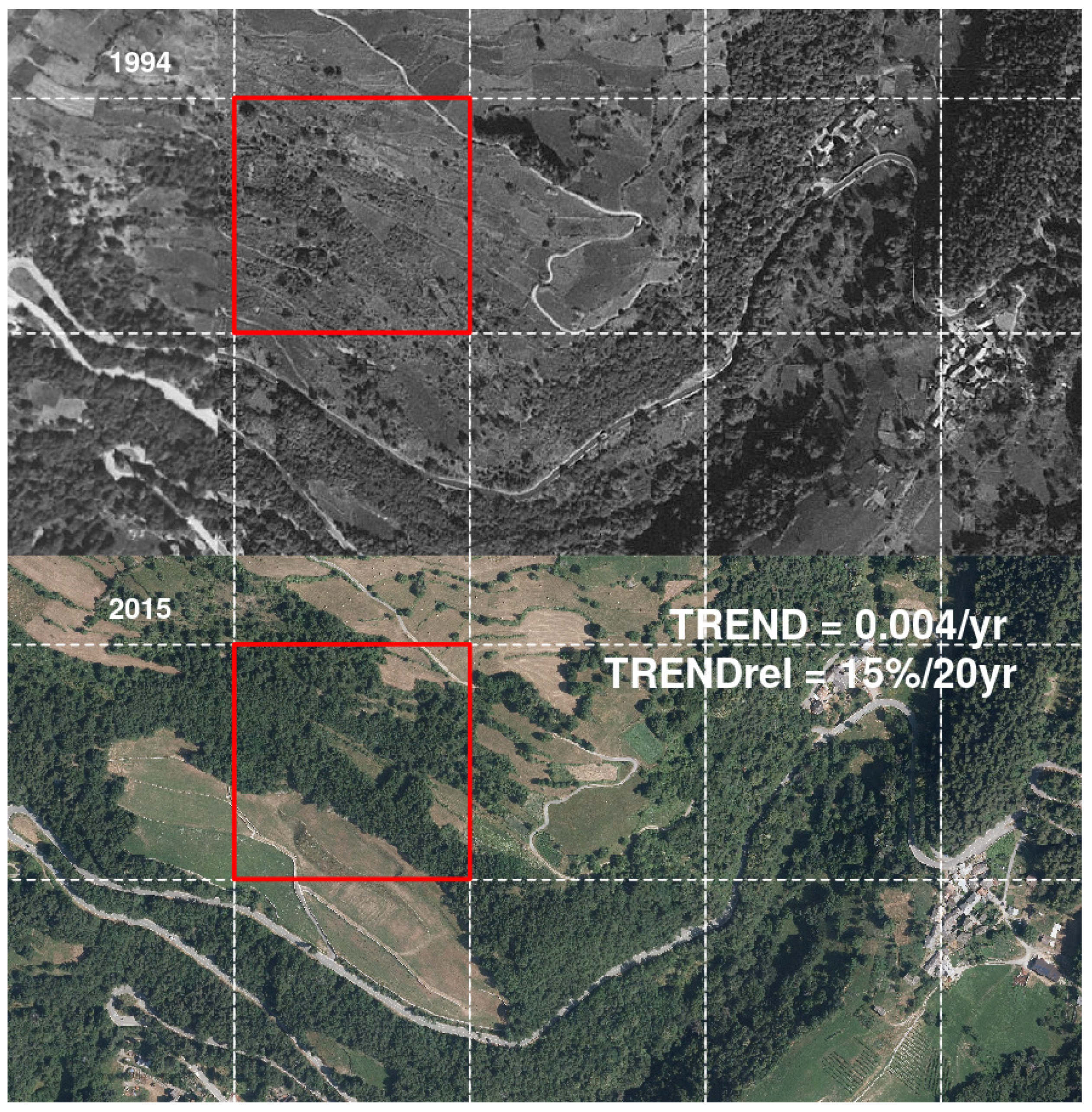
- What is the magnitude of greening trends in the Western Alps when the role of the disturbance is accounted for?
- (2)
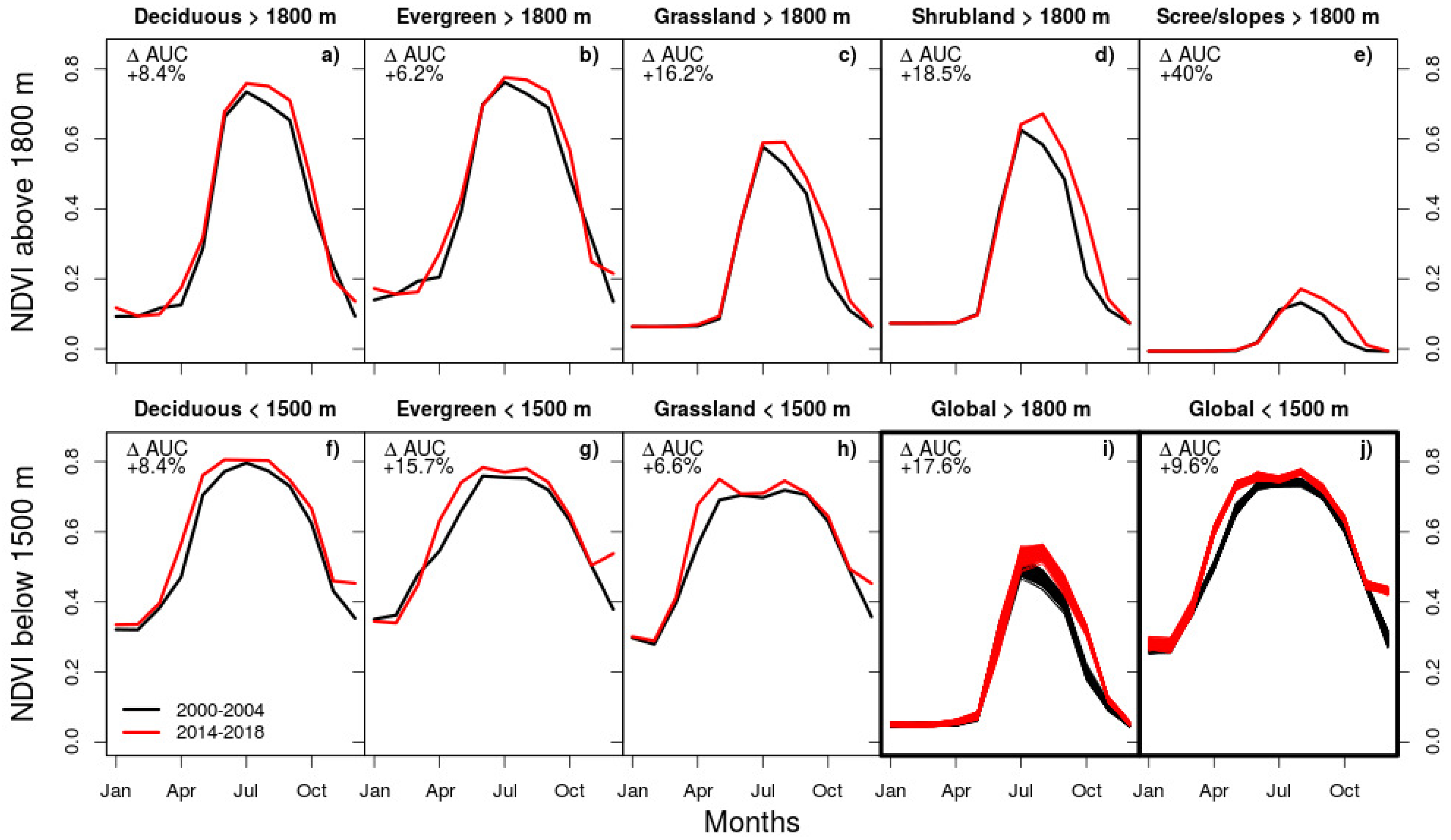
- What are the mechanisms and causes of the spatial patterns of greening across plant types, elevation gradients, and seasons?
2. Materials and Methods
2.1. Study Area, Climate Data, and Vegetation Mapping
2.2. Satellite Data
2.3. Data Analysis
3. Results
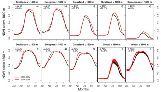
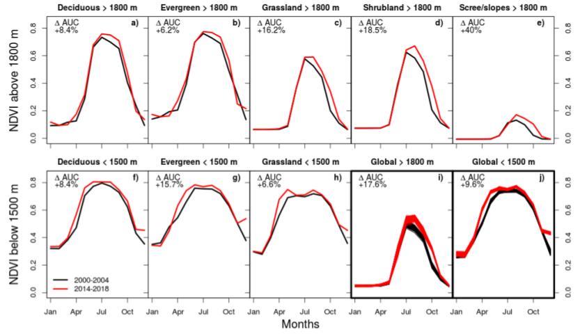
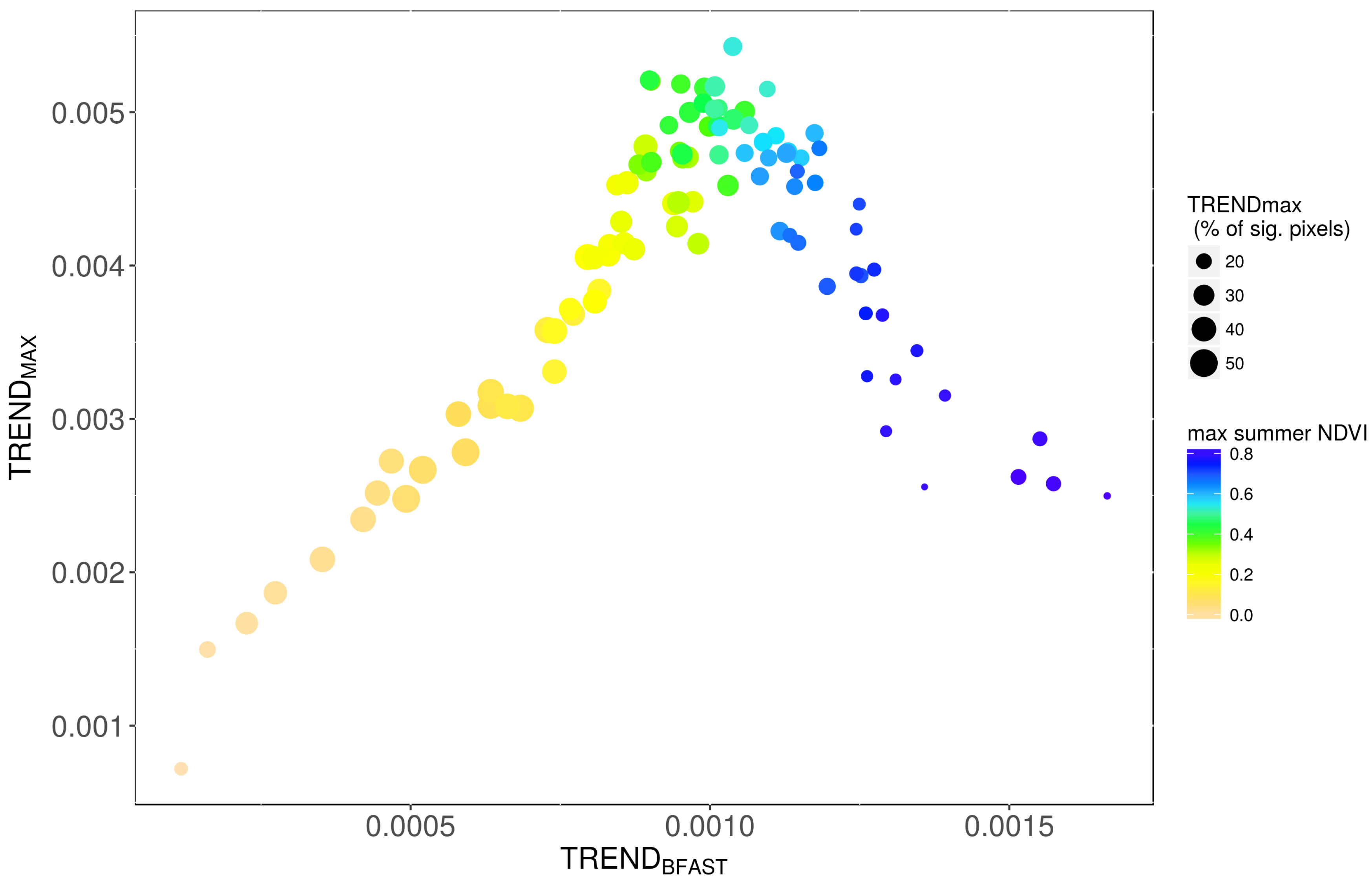
3.1. Comparison of TREND and TREND
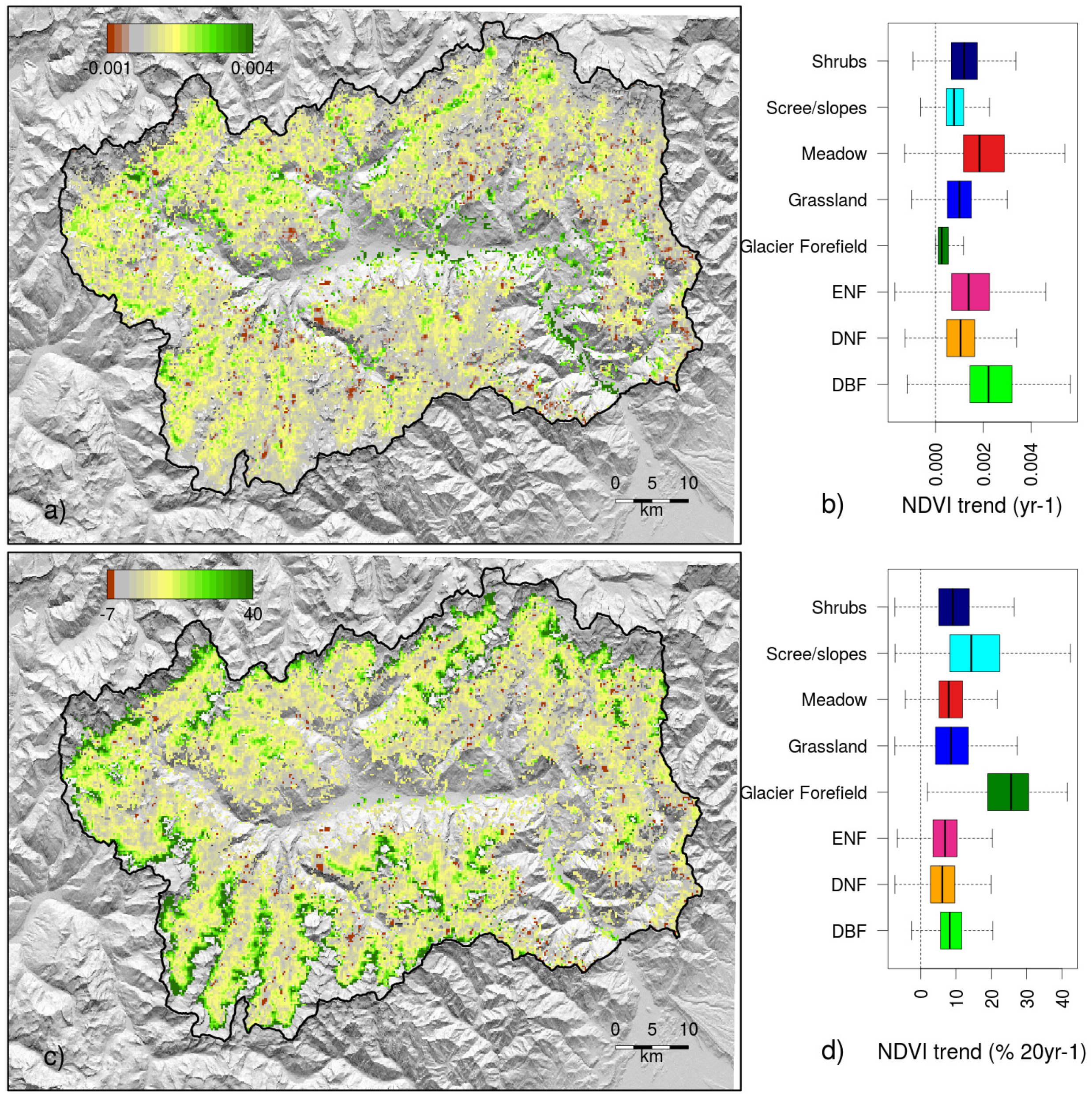
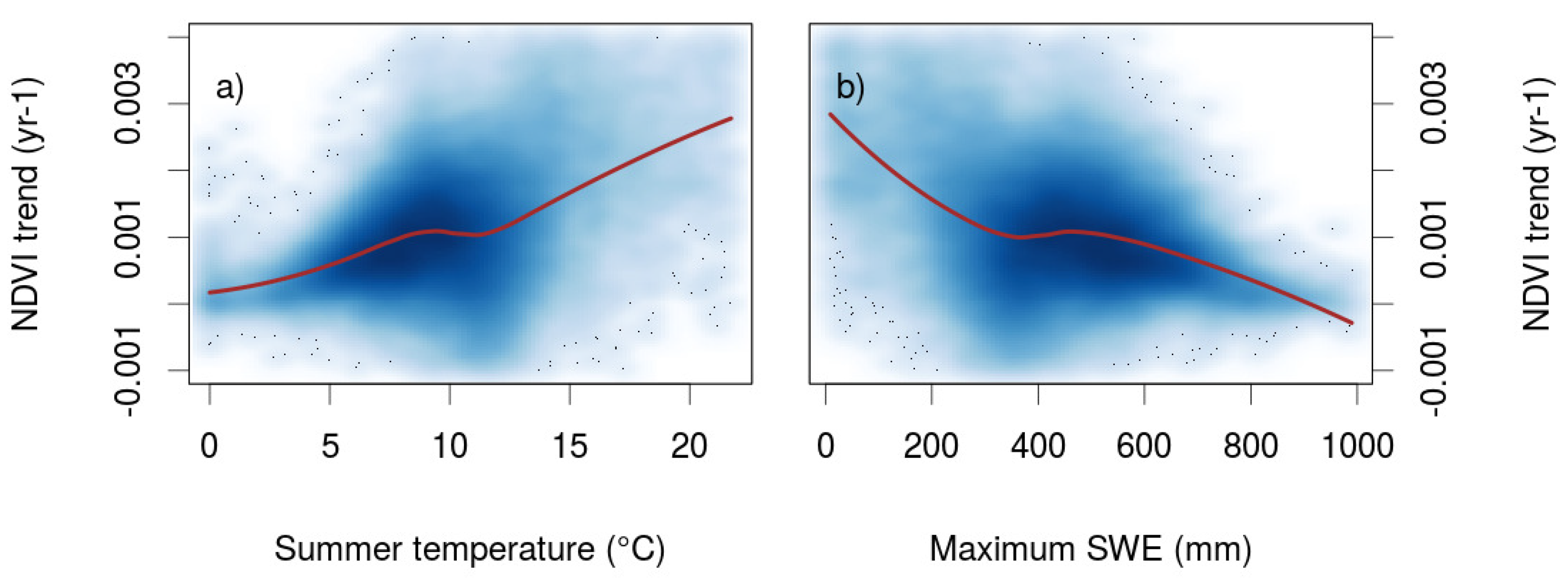
3.2. Factors Controlling NDVI Trends
4. Discussion
4.1. Methodological Considerations
4.2. Controls and Mechanisms of Greening
4.3. Magnitude of Trends and Spatial Patterns
5. Conclusions
Author Contributions
Funding
Acknowledgments
Conflicts of Interest
References
- Huang, K.; Xia, J.; Wang, Y.; Ahlstrom, A.; Chen, J.; Cook, R.B.; Cui, E.; Fang, Y.; Fisher, J.B.; Nicole Huntzinger, D.; et al. Enhanced peak growth of global vegetation and its key mechanisms. Nat. Ecol. Evol. 2018, 2. [Google Scholar] [CrossRef] [PubMed]
- Zhu, Z.; Piao, S.; Myneni, R.B.; Huang, M.; Zeng, Z.; Canadell, J.G.; Ciais, P.; Sitch, S.; Friedlingstein, P.; Arneth, A.; et al. Greening of the Earth and its drivers. Nat. Clim. Chang. 2016, 6. [Google Scholar] [CrossRef]
- Keenan, T.; Gray, J.; Friedl, M.A.; Toomey, M.; Bohrer, G.; Hollinger, D.; Munger, J.; O’Keefe, J.; Peter Schmid, H.; Sue Wing, I.; et al. Net carbon uptake has increased through warming-induced changes in temperate forest phenology. Nat. Clim. Chang. 2014, 4, 598–604. [Google Scholar] [CrossRef]
- Beer, C.; Reichstein, M.; Tomelleri, E.; Ciais, P.; Jung, M.; Carvalhais, N.; Rodenbeck, C.; Arain, M.; Baldocchi, D.; Bonan, G.; et al. Terrestrial Gross Carbon Dioxide Uptake: Global Distribution and Covariation with Climate. Science 2010, 329, 834–838. [Google Scholar] [CrossRef] [PubMed]
- Keenan, T.; Riley, W. Greening of the land surface in the World’s cold regions consistent with recent warming. Nat. Clim. Chang. 2018, 8, 825. [Google Scholar] [CrossRef] [PubMed]
- Barichivich, J.; Briffa, K.R.; Myneni, R.B.; Osborn, T.J.; Melvin, T.M.; Ciais, P.; Piao, S.; Tucker, C. Large-scale variations in the vegetation growing season and annual cycle of atmospheric CO2 at high northern latitudes from 1950 to 2011. Glob. Chang. Biol. 2013, 19, 3167–3183. [Google Scholar] [CrossRef]
- Park, T.; Chen, C.; Macias-Fauria, M.; Tømmervik, H.; Choi, S.; Winkler, A.; Bhatt, U.S.; Walker, D.A.; Piao, S.; Brovkin, V.; et al. Changes in timing of seasonal peak photosynthetic activity in northern ecosystems. Glob. Chang. Biol. 2019, 25, 2382–2395. [Google Scholar] [CrossRef]
- Macias-Fauria, M.; Forbes, B.; Zetterberg, P.; Kumpula, T. Eurasian Arctic greening reveals teleconnections andthe potential for structurally novel ecosystems. Nat. Clim. Chang. 2012, 2, 613–618. [Google Scholar] [CrossRef]
- Croci-Maspoli, M.; Schär, C.; Fischer, A.; Strassmann, K.; Scherrer, S.; Schwierz, C.; Knutti, R.; Kotlarski, S.; Rajczak, J.; Fischer, E.; et al. CH2018-Climate Scenarios for Switzerland-Technical Report; National Centre for Climate Services: Zurich, Switzerland, 2018; 271p. [Google Scholar]
- Gobiet, A.; Kotlarski, S.; Beniston, M.; Heinrich, G.; Rajczak, J.; Stoffel, M. 21st century climate change in the European Alps—A review. Sci. Total Environ. 2014, 493, 1138–1151. [Google Scholar] [CrossRef]
- Durand, Y.; Giraud, G.; Laternser, M.; Etchevers, P.; Mérindol, L.; Lesaffre, B. Reanalysis of 47 Years of Climate in the French Alps (1958–2005): Climatology and Trends for Snow Cover. J. Appl. Meteorol. Climatol. 2009, 48, 2487–2512. [Google Scholar] [CrossRef]
- Hüsler, F.; Jonas, T.; Riffler, M.; Musial, J.P.; Wunderle, S. A satellite-based snow cover climatology (1985–2011) for the European Alps derived from AVHRR data. Cryosphere 2014, 8, 73–90. [Google Scholar] [CrossRef]
- Cazzolla Gatti, R.; Dudko, A.; Lim, A.; Velichevskaya, A.I.; Lushchaeva, I.V.; Pivovarova, A.V.; Ventura, S.; Lumini, E.; Berruti, A.; Volkov, I.V. The last 50 years of climate-induced melting of the Maliy Aktru glacier (Altai Mountains, Russia) revealed in a primary ecological succession. Ecol. Evol. 2018, 8, 7401–7420. [Google Scholar] [CrossRef] [PubMed]
- Rogora, M.; Frate, L.; Carranza, M.; Freppaz, M.; Stanisci, A.; Bertani, I.; Bottarin, R.; Brambilla, A.; Canullo, R.; Carbognani, M.; et al. Assessment of climate change effects on mountain ecosystems through a cross-site analysis in the Alps and Apennines. Sci. Total Environ. 2018, 624. [Google Scholar] [CrossRef] [PubMed]
- Harsch, M.A.; Hulme, P.E.; McGlone, M.S.; Duncan, R.P. Are treelines advancing? A global meta-analysis of treeline response to climate warming. Ecol. Lett. 2009, 12, 1040–1049. [Google Scholar] [CrossRef]
- Bolton, D.K.; Coops, N.C.; Hermosilla, T.; Wulder, M.A.; White, J.C. Evidence of vegetation greening at alpine treeline ecotones: Three decades of Landsat spectral trends informed by lidar-derived vertical structure. Environ. Res. Lett. 2018, 13, 084022. [Google Scholar] [CrossRef]
- Steinbauer, M.; Grytnes, J.A.; Jurasinski, G.; Kulonen, A.; Lenoir, J.; Pauli, H.; Rixen, C.; Winkler, M.; Bardy-Durchhalter, M.; Barni, E.; et al. Accelerated increase in plant species richness on mountain summits is linked to warming. Nature 2018, 556. [Google Scholar] [CrossRef]
- Carlson, B.Z.; Corona, M.C.; Dentant, C.; Bonet, R.; Thuiller, W.; Choler, P. Observed long-term greening of alpine vegetation—A case study in the French Alps. Environ. Res. Lett. 2017, 12, 114006. [Google Scholar] [CrossRef]
- Corona-Lozada, M.; Morin, S.; Choler, P. Drought offsets the positive effect of summer heat waves on the canopy greenness of mountain grasslands. Agric. For. Meteorol. 2019, 276, 107617. [Google Scholar] [CrossRef]
- Asam, S.; Callegari, M.; Matiu, M.; Fiore, G.; Gregorio, L.; Jacob, A.; Menzel, A.; Zebisch, M.; Notarnicola, C. Relationship between Spatiotemporal Variations of Climate, Snow Cover and Plant Phenology over the Alps—An Earth Observation-Based Analysis. Remote Sens. 2018, 10, 1757. [Google Scholar] [CrossRef]
- de Jong, R.; Verbesselt, J.; Schaepman, M.E.; de Bruin, S. Trend changes in global greening and browning: Contribution of short-term trends to longer-term change. Glob. Chang. Biol. 2012, 18, 642–655. [Google Scholar] [CrossRef]
- Emmett, K.D.; Renwick, K.M.; Poulter, B. Disentangling Climate and Disturbance Effects on Regional Vegetation Greening Trends. Ecosystems 2019, 22, 873–891. [Google Scholar] [CrossRef]
- Verbesselt, J.; Hyndman, R.; Newnham, G.; Culvenor, D. Detecting Trend and Seasonal Changes in Satellite Image Time Series. Remote Sens. Environ. 2010, 114, 106–115. [Google Scholar] [CrossRef]
- Verbesselt, J.; Hyndman, R.; Zeileis, A.; Culvenor, D. Phenological Change Detection while Accounting for Abrupt and Gradual Trends in Satellite Image Time Series. Remote Sens. Environ. 2010, 114, 2970–2980. [Google Scholar] [CrossRef]
- Geng, L.; Che, T.; Wang, X.; Wang, H. Detecting Spatiotemporal Changes in Vegetation with the BFAST Model in the Qilian Mountain Region during 2000–2017. Remote Sens. 2019, 11, 103. [Google Scholar] [CrossRef]
- Silvestro, F.; Gabellani, S.; Rudari, R.; Delogu, F.; Laiolo, P.; Boni, G. Uncertainty reduction and parameter estimation of a distributed hydrological model with ground and remote-sensing data. Hydrol. Earth Syst. Sci. 2015, 19, 1727–1751. [Google Scholar] [CrossRef]
- Silvestro, F.; Gabellani, S.; Delogu, F.; Rudari, R.; Boni, G. Exploiting remote sensing land surface temperature in distributed hydrological modelling: The example of the Continuum model. Hydrol. Earth Syst. Sci. 2013, 17, 39–62. [Google Scholar] [CrossRef]
- Deardorff, J.W. Dependence of air-sea transfer coefficients on bulk stability. J. Geophys. Res. (1896–1977) 1968, 73, 2549–2557. [Google Scholar] [CrossRef]
- Evans, D. The Habitats of the European Union Habitats Directive. Biol. Environ. Proc. R. Irish Acad. 2006, 106, 167–173. [Google Scholar] [CrossRef]
- Comission DG Environment, E. The Interpretation Manual of European Union Habitats—EUR27. Eur. Comm. DG Environ. Nat. Biodivers. 2007, 27, 368. [Google Scholar]
- Vermote, E. MOD09Q1 MODIS/Terra Surface Reflectance 8-Day L3 Global 250m SIN Grid V006. NASA EOSDIS Land Processes DAAC. 2015. Available online: https://doi.org/10.5067/MODIS/MOD09Q1.006 (accessed on 5 January 2019).
- Busetto, L.; Ranghetti, L. MODIStsp: An R package for preprocessing of MODIS Land Products time series. Comput. Geosci. 2016, 97, 40–48. [Google Scholar] [CrossRef]
- Busetto, L.; Colombo, R.; Migliavacca, M.; Cremonese, E.; Meroni, M.; Galvagno, M.; Rossini, M.; Siniscalco, C.; Morra Di Cella, U.; Pari, E. Remote sensing of larch phenological cycle and analysis of relationships with climate in the Alpine region. Glob. Chang. Biol. 2010. [Google Scholar] [CrossRef]
- Choler, P. Growth response of temperate mountain grasslands to inter-annual variations in snow cover duration. Biogeosciences 2015, 12, 3885–3897. [Google Scholar] [CrossRef]
- Sen, K.P. Estimates of the Regression Coefficient Based on Kendall’s Tau. J. Am. Stat. Assoc. 1968, 63. [Google Scholar] [CrossRef]
- Cleveland, B.R.; Cleveland, S.W.; McRae, E.J.; Terpenning, I. STL: A Seasonal-Trend Decomposition Procedure Based on Loess. J. Off. Stat. 1990, 6, 3–33. [Google Scholar]
- Wright, M.N.; Ziegler, A. ranger: A Fast Implementation of Random Forests for High Dimensional Data in C++ and R. J. Stat. Softw. 2017, 77, 1–17. [Google Scholar] [CrossRef]
- Kuhn, M. Caret: Classification and Regression Training; R Package Version 6.0-79. 2018. Available online: http://adsabs.harvard.edu/abs/2015ascl.soft05003K (accessed on 1 October 2019).
- R Core Team. R: A Language and Environment for Statistical Computing; R Foundation for Statistical Computing: Vienna, Austria, 2019. [Google Scholar]
- Geurts, P.; Ernst, D.; Wehenkel, L. Extremely Randomized Trees. Mach. Learn. 2006, 63, 3–42. [Google Scholar] [CrossRef]
- McCune, B.; Keon, D. Equations for potential annual direct incident radiation and heat load. J. Veg. Sci. 2002, 13, 603–606. [Google Scholar] [CrossRef]
- Richardson, A.D.; Keenan, T.F.; Migliavacca, M.; Ryu, Y.; Sonnentag, O.; Toomey, M. Climate change, phenology, and phenological control of vegetation feedbacks to the climate system. Agric. For. Meteorol. 2013, 169, 156–173. [Google Scholar] [CrossRef]
- Migliavacca, M.; Cremonese, E.; Colombo, R.; Busetto, L.; Galvagno, M.; Ganis, L.; Meroni, M.; Pari, E.; Rossini, M.; Siniscalco, C.; et al. European larch phenology in the Alps: Can we grasp the role of ecological factors by combining field observations and inverse modelling? Int. J. Biometeorol. 2008, 52, 587–605. [Google Scholar] [CrossRef]
- Migliavacca, M.; Galvagno, M.; Cremonese, E.; Rossini, M.; Meroni, M.; Sonnentag, O.; Cogliati, S.; Manca, G.; Diotri, F.; Busetto, L.; et al. Using digital repeat photography and eddy covariance data to model grassland phenology and photosynthetic CO2 uptake. Agric. For. Meteorol. 2011, 151, 1325–1337. [Google Scholar] [CrossRef]
- Buermann, W.; Forkel, M.; O’Sullivan, M.; Sitch, S.; Friedlingstein, P.; Haverd, V.; Jain, A.K.; Kato, E.; Kautz, M.; Lienert, S.; et al. Widespread seasonal compensation effects of spring warming on northern plant productivity. Nature 2018, 562. [Google Scholar] [CrossRef] [PubMed]
- Klein, G.; Vitasse, Y.; Rixen, C.; Marty, C.; Rebetez, M. Shorter snow cover duration since 1970 in the Swiss Alps due to earlier snowmelt more than to later snow onset. Clim. Chang. 2016. [Google Scholar] [CrossRef]
- Menzel, A.; Sparks, T.; Estrella, N.; Koch, E.; Aasa, A.; Ahas, R.; Alm-Kubler, K.; Bissolli, P.; Braslaskva, O.; Briede, A.; et al. European phenological response to climate change matches the warming pattern. Glob. Chang. Biol. 2006, 12, 1969–1976. [Google Scholar] [CrossRef]
- Parmesan, C.; Yohe, G. A globally coherent fingerprint of climate change impacts across natural systems. Nature 2003, 421, 37–42. [Google Scholar] [CrossRef] [PubMed]
- Way, D.A.; Montgomery, R.A. Photoperiod constraints on tree phenology, performance and migration in a warming world. Plant Cell Environ. 2015, 38, 1725–1736. [Google Scholar] [CrossRef]
- Ren, S.; Yi, S.; Peichl, M.; Wang, X. Diverse Responses of Vegetation Phenology to Climate Change in Different Grasslands in Inner Mongolia during 2000–2016. Remote Sens. 2018, 10, 17. [Google Scholar] [CrossRef]
- Eichel, J.; Krautblatter, M.; Schmidtlein, S.; Dikau, R. Biogeomorphic interactions in the Turtmann glacier forefield, Switzerland. Geomorphology 2013, 201, 98–110. [Google Scholar] [CrossRef]
- D’Amico, M.E.; Freppaz, M.; Filippa, G.; Zanini, E. Vegetation influence on soil formation rate in a proglacial chronosequence (Lys Glacier, NW Italian Alps). CATENA 2014, 113, 122–137. [Google Scholar] [CrossRef]
- Grabherr, G.; Gottfried, M.; Pauli, H. Climate Change Impacts in Alpine Environments. Geogr. Compass 2010, 4, 1133–1153. [Google Scholar] [CrossRef]
- Améztegui, A.; Brotons, L.; Coll, L. Land-use changes as major drivers of mountain pine (Pinus uncinata Ram.) expansion in the Pyrenees. Glob. Ecol. Biogeogr. 2010, 19, 632–641. [Google Scholar] [CrossRef]
- Elmendorf, S.C.; Henry, G.; Hollister, R.; Björk, R.; Boulanger-Lapointe, N.; Cooper, E.J.; Cornelissen, J.; Day, T.; Dorrepaal, E.; Elumeeva, T.; et al. Plot-scale evidence of tundra vegetation change and links to recent summer warming. Nat. Clim. Chang. 2012, 2. [Google Scholar] [CrossRef]
- Koch, B.; Edwards, P.J.; Blanckenhorn, W.U.; Walter, T.; Hofer, G. Shrub Encroachment Affects the Diversity of Plants, Butterflies, and Grasshoppers on Two Swiss Subalpine Pastures. Arctic Antarct. Alp. Res. 2015, 47, 345–357. [Google Scholar] [CrossRef]


| Variable Type | Details | Acronyms |
|---|---|---|
| Thermal conditions | Mean summer temperature, temperature trend, heat load index [41] | Tsummer, Ttrend, hli |
| Water status | Summer water balance, maximum snow water equivalent, annual and summer precipitation | PmET, maxSwe (snow water equivalent), P, Psummer |
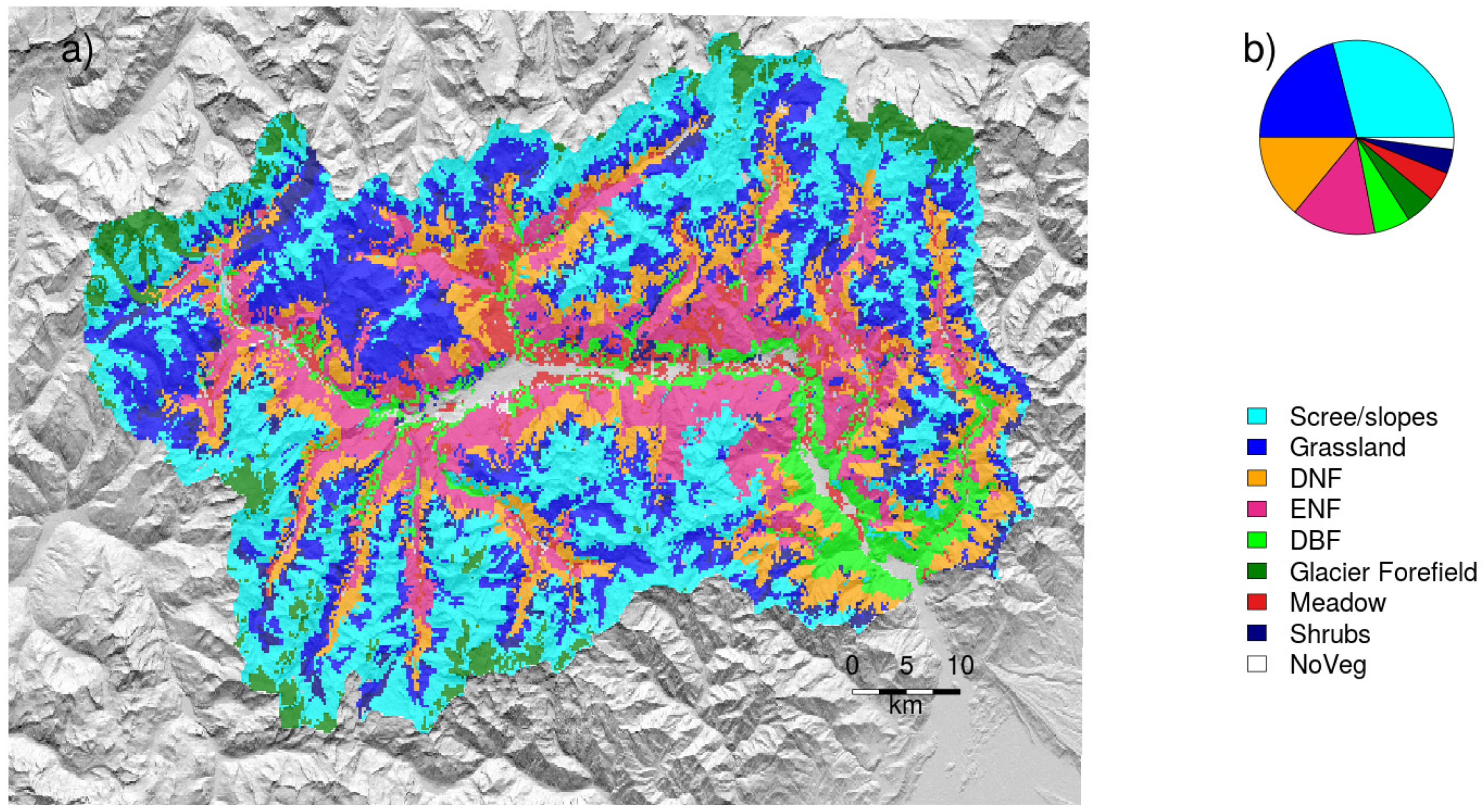
| Vegetation type | plant macrotype as in Figure 1 and mean max normalized difference vegetation index (NDVI) | pft, maxNDVI |
| Plant Macro-Type | % Pixels with Significant Trend | % Disturbed Pixels below 1500 m | % Disturbed Pixels above 1500 m | Total Disturbed Pixels |
|---|---|---|---|---|
| Deciduous broadleaf forest | 22 | 75 | 2 | 77 |
| Meadow | 35 | 53 | 11 | 65 |
| Evergreen | 30 | 37 | 32 | 69 |
| Deciduous needleleaf forest | 61 | 9 | 28 | 37 |
| Shrubs | 85 | 5 | 10 | 15 |
| Grassland | 87 | 2 | 10 | 12 |
| Scree/slopes | 76 | 1 | 22 | 23 |
| Glacier Forefield | 33 | n.a. | 56 | 56 |
| Total | 63 | 14 (69) | 17 (21) | 31 |
| Statistics | TREND | TREND |
|---|---|---|
| 10th quantile | 1.88 | 0.09 |
| 25th quantile | 2.78 | 0.46 |
| Median | 3.90 | 0.94 |
| 75th quantile | 5.26 | 1.51 |
| 90th quantile | 6.66 | 2.17 |
| Sig. pixels (%) | 16 | 63 |
© 2019 by the authors. Licensee MDPI, Basel, Switzerland. This article is an open access article distributed under the terms and conditions of the Creative Commons Attribution (CC BY) license (http://creativecommons.org/licenses/by/4.0/).
Share and Cite
Filippa, G.; Cremonese, E.; Galvagno, M.; Isabellon, M.; Bayle, A.; Choler, P.; Carlson, B.Z.; Gabellani, S.; Morra di Cella, U.; Migliavacca, M. Climatic Drivers of Greening Trends in the Alps. Remote Sens. 2019, 11, 2527. https://doi.org/10.3390/rs11212527
Filippa G, Cremonese E, Galvagno M, Isabellon M, Bayle A, Choler P, Carlson BZ, Gabellani S, Morra di Cella U, Migliavacca M. Climatic Drivers of Greening Trends in the Alps. Remote Sensing. 2019; 11(21):2527. https://doi.org/10.3390/rs11212527
Chicago/Turabian StyleFilippa, Gianluca, Edoardo Cremonese, Marta Galvagno, Michel Isabellon, Arthur Bayle, Philippe Choler, Bradley Z. Carlson, Simone Gabellani, Umberto Morra di Cella, and Mirco Migliavacca. 2019. "Climatic Drivers of Greening Trends in the Alps" Remote Sensing 11, no. 21: 2527. https://doi.org/10.3390/rs11212527
APA StyleFilippa, G., Cremonese, E., Galvagno, M., Isabellon, M., Bayle, A., Choler, P., Carlson, B. Z., Gabellani, S., Morra di Cella, U., & Migliavacca, M. (2019). Climatic Drivers of Greening Trends in the Alps. Remote Sensing, 11(21), 2527. https://doi.org/10.3390/rs11212527