Abstract
This paper proposes a multimodal and multi-task deep-learning model for instantaneous precipitation rate estimation. Using both thermal infrared satellite radiometer and automatic rain gauge measurements as input, our encoder–decoder convolutional neural network performs a multiscale analysis of these two modalities to estimate simultaneously the rainfall probability and the precipitation rate value. Precipitating pixels are detected with a Probability Of Detection (POD) of 0.75 and a False Alarm Ratio (FAR) of 0.3. Instantaneous precipitation rate is estimated with a Root Mean Squared Error (RMSE) of 1.6 mm/h.
1. Introduction
Instantaneous precipitation rate estimation is an important problem for meteorological, climatological and hydrological applications. It also forms the basis for short-term precipitation forecasting, also called nowcasting [1].
Rain gauges are considered to be the reference devices for the measurement of the amount of precipitation at ground level. Climatological rain gauges are simple recipients, manually read out once per day. There are also networks of automatic stations, able to report rainfall quantity every 5 or 10 min. The main drawback of rain gauges is their lack of spatial representativity, being only point measurements.
Ground-based radars scan the atmosphere by emitting an electromagnetic beam and measuring its reflection caused by particles in the air. The amount of beam reflection depends on both the density and the size of the particles, allowing estimation of the amount of precipitation. By scanning the atmosphere at 360 degrees around them at different heights, radars are able to produce rainfall estimates in a radius of about 100 to 150 km at a high spatial resolution (∼1 km) and temporal resolution (∼5 min). This good spatial and temporal resolution makes them a popular tool for instantaneous rain rate estimation and nowcasting. However, radars come with a limited spatial coverage and a large amount of error sources, e.g., the uncertainty about the droplets size distribution and the hydrometeors type (rain, hail, snow), beam blockage by obstacles (mountains, hills, wind turbines), electromagnetic interferences and ground clutters. Quantitative Precipitation Estimation (QPE) from radar observations requires a complex processing including a calibration with rain gauges [2].
Satellite radiometers are passive measurement devices measuring the earth’s electromagnetic radiation at different wavelengths. Estimating precipitation from them is more difficult than with radars but they have the advantage of having a larger spatial coverage, e.g., the sea, the mountains and all isolated regions with no radars available. Operational satellite precipitation remote sensing has been mostly relying on a combination of microwave instruments on Low Earth Orbit (LEO) satellites and geostationary window infrared images at wavelengths around 11 micron [3,4,5]. Microwave measurements are directly related to large-size hydrometeors since non-precipitating small-size cloud particles are transparent for microwave radiation, while the large-size hydrometeors are attenuating the microwave radiation. The direct observation of precipitation at the LEO overpass times are then extrapolated in time through their correlation with geostationary window brightness temperatures. There is a negative correlation between window infrared cloud top brightness temperature and the amount of precipitation.
For the best estimation of precipitation from geostationary satellite imagery, the three independent cloud physical properties needed are cloud optical thickness, cloud top temperature, and cloud particle size [6,7]. In particular the cloud particle size is the most relevant parameter, since it allows remote sensing of the growth of non-precipitating small-size cloud particles into precipitating large-size hydrometeors. The remote sensing of cloud particle size requires the use of near-infrared measurements. These near-infrared measurements were not present on the Geostationary Earth Orbiting (GEO) Meteosat First Generation, but they are on the GEO Meteosat Second Generation (MSG). This allowed the development of a ’direct’ estimation of precipitation from MSG, which was pioneered by [8]. In this study, a daytime only retrieval of the particle size and optical depth was used, so only daytime precipitation estimates were obtained. As in most studies made on precipitation estimation from satellite imager data [6,7], the method in [8] relies on many assumptions made on the underlying physical processes describing precipitation, and in the end, different parameters still need to be calibrated on ground truth measurements. These methods provide interpretable results, but their performance is limited by the assumptions made on the physical models behind these algorithms.
Instead, a direct relation between the satellite data and observed precipitations can be made using Machine Learning (ML) techniques, reducing the need for any physical assumption. The fully connected Neural Network (NN) developed in [4] is a pioneer in the ML approach, but relies on microwave measurements made from LEO satellites suffering from low temporal resolution. Thanks to the near-infrared measurements from MSG, more recent studies have been developed to use exclusively this GEO satellite and benefit from his high temporal resolution (15 min for the complete disk scan and 5 min for the rapid scan of Europe) and spatial resolution (3 km at nadir). Using the MSG data, [9] developed a 24 h precipitation estimation method relying on random forest and [10] used a fully connected neural network.
However, all these studies used radar data recalibrated on rain gauge data as training target, which is not as accurate as rain gauge measurements. Also, none of these studies used modern Deep-Learning (DL) techniques [11], where multiple processing layers representing multiple levels of abstraction exist between the input and the output of a DL NN.
The differences and complementarities in QPE capabilities between rain gauges, radars and satellite radiometers favors the use of multimodal approaches. For example, methods combining radars with rain gauges are often used and offer better performance than the use of radars or gauges alone [12]. In this paper, we will focus on the combination of geostationary satellite radiometers, providing wide spatial coverage of uniform quality, and rain gauges, providing a local ground truth. The idea behind this multimodal merging is that rain gauges provide point measurements of the precipitation field, from which interpolation accuracy is limited by both the sparsity of the rain gauges and the spatial variability of the precipitation event. On the other hand, the higher spatial resolution of the satellite data provides information where rain gauges are missing. With the correct DL architecture, the satellite images can serve as a guided filter for the rain gauge measurements, allowing increase of the resolution and accuracy compared to a simple spatial interpolation of the rain gauge measurements.
Compared to the above-mentioned studies, we propose to introduce some key innovations:
- As satellite inputs, we will only use the three Meteosat Second Generation (MSG) [13] Spinning Enhanced Visible and Infrared Imager (SEVIRI) spectral channels that contain the information on the optical properties that are relevant for precipitation estimation, and that are useable in all illumination conditions. These channels are the 8.7, 10.8 and 12.0 micron channels. These are the channels used in the well-known “24 h microphysics RGB” [7].
- We will also include automatic rain gauge measurements as an additional input to our model. Rain gauge interpolation with geostatistical method, e.g., kriging [14], is the most widespread method for precipitation estimation on long periods (≥1 day). For instantaneous precipitation estimation, rain gauges interpolation becomes ineffective because the spatial variability becomes too large compared to the density of even the densest network of automatic rain gauges. In our case, our model will learn to use the satellite data as a guided filter to further improve the rain gauge interpolation and increase its spatial resolution.
- We will use a DL NN, consisting of a multiscale convolutional network. In our design we follow a multiscale encoder–decoder paradigm that consists of several resolution-reduction steps in which low resolution contextual information is derived, followed by several resolution-enhancement steps, where the final output has the same resolution as the input. The proposed multiscale convolutional network model was motivated by the high performance and accuracy obtained with the Hourglass-Shape Network (HSN) in [15]. The design of HSN proved to be particularly efficient for semantic segmentation of aerial images.
- We will train our DL model with rain gauges measurements as target data, eliminating the intermediate step of using radar data recalibrated by rain gauges. The rain gauge data was provided by different networks of rain gauges located in Belgium, the Netherlands and Germany.
- We use multi-task learning to improve performance and to allow both precipitation detection and precipitation rate estimation at once [16]. This lies in contrast to single-task learning typically employed in encoder–decoder architectures, including the previous HSN design [15].
- For the same network architecture we will separately use (1) only rain gauges; (2) only satellite data; (3) both rain gauges and satellite data as input. This will allow the separate quantification of the benefits of both modalities (rain gauges and satellite data), and the added value of their combination.
- The performance of the three models mentioned above will be evaluated on an independent automatic rain gauge dataset for instantaneous precipitation rate estimation, and on daily measurements coming from manually daily checked gauges. The performance will also be compared to the kriging interpolation of the rain gauges, which is the traditional geostatistical method for rain gauge interpolation.
The paper is structured as follows. Section 2 describes the source and the preparation of the data. In Section 3, we describe in more detail how our data is used as input by our model, the data splitting into a training, a validation and a test set, the model architecture and the training strategy. In Section 4, the performance of our model is assessed for both instantaneous precipitation rate and for daily rainfall quantity estimation. Then, we discuss these results and compare our work to previous studies in Section 5. Finally, we draw conclusions of our work in Section 6.
2. Data
2.1. SEVIRI Satellite Images
The SEVIRI radiometer on MSG performs a scan of the earth every 15 min producing 12 different images; 11 of these images are sensible to wavelengths ranging from 0.6 μm to 14 μm and have a spatial resolution of 3 km at nadir. The 12th scan has a higher resolution of 1 km at nadir, and is sensitive to visible light (0.5–0.9 μm). We used the measurements from years 2016 to 2018, made by both MSG-3 and MSG-4 (MSG-4 replaced MSG-3 in early 2018), which were located in a geostationary orbit at (0°N, 0°E).
For this study, we only used the Brightness Temperature (BT) from three different infrared channels: 8.7, 10.8, and 12.0 μm, because those are the three channels (1) that are directly related to the three physical cloud properties that are relevant for precipitation estimation—namely cloud optical thickness, cloud top temperature and particle size—and (2) that have a similar behavior during daytime and night time [7] (Figure 1). With these three channels we can discriminate all possible precipitation types, and quantify the precipitation amount. Convective precipitation can easily be recognized using only cloud top brightness temperature. The most challenging case is the one of so-called warm rain, in which the inclusion of cloud particle size is essential [17].
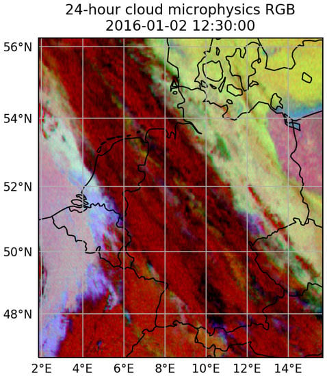
Figure 1.
The 24 h cloud microphysics RGB image made from the 8.7, 10.8, and 12.0 μm channels spanning our studied area, i.e., Belgium, the Netherlands and Germany. This image allows distinguishing of different microphysical properties of the clouds. The red component relates to cloud optical thickness, the green component relates to cloud particle size and the blue component relates to the cloud top temperature. Red colors in the RGB indicates thick cold clouds with large particles, which are likely to produce precipitation.
The viewing angle from the geostationary orbit of MSG results in a non-negligible geometrical deformation around the latitudes of interest (between 47°N and 56°N). To remove this deformation, the satellite images are reprojected on an equal area sinusoidal grid with 3 km resolution. For the interpolation, we used the griddata package from the Python library Scipy, constructing a piecewise cubic interpolating Bezier polynomial on each triangle, using a Clough–Tocher scheme [18].
2.2. Rain Gauges
We used data from the automatic rain gauges located in Belgium, Netherlands and Germany as training target for our model. These rain gauges are part of different networks:
- Belgium: Royal Meteorological Institute of Belgium (RMIB), Société bruxelloise de Gestion de l’Eau (SBGE), Vlaamse Milieumaatschappij (VMM), Service d’Etude Hydrologique (SETHY).
- Netherlands: Koninklijk Nederlands Meteorologisch Instituut (KNMI).
- Germany: Deutscher Wetterdienst (DWD).
In total, the measurements from 1176 different rain gauges were used.
All these rain gauges measure rain accumulation during a period from 5 up to 10 min. From the precipitation quantity measurements, we estimated the average rain rate precipitation in mm/h and set a minimum and maximum between 0 and 100 mm/h. The rain rate was then interpolated linearly on the same temporal grid as the SEVIRI scans, using only measurements that are close enough temporally to the targeted timestamps. The rain gauges were then assigned to the location of the closest pixel on the interpolated satellite images. Using this scheme, a few rain gauges are sharing the same pixel. For these gauges, the measurements were aggregated by taking their mean, reducing the number of gauges to 1166.
Additionally, we used the RMIB climatological network of rain gauges for the performance evaluation of our models. This network consists of more than 250 manual rain gauges located in Belgium that provide the daily total precipitation.
2.3. Topography
The weather being influenced by the topography, we also added it to the model’s inputs. The data was provided by the Shuttle Radar Topography Mission (SRTM).
3. Methodology
To develop and test our method, we used the common ML approach which consists of using three independent datasets: a training set, a validation set and a test set. The training set, as denoted by its name, is used to train the model by optimizing its learnable parameters with the back-propagation algorithm [11]. To evaluate our model performance, we use an independent validation dataset, to assert its ability to generalize well to new data, i.e., to make sure that our model is not overfitting the training data. This happens when the model is performing well on the data used during training but performs poorly on new unseen data. Evaluating the performance on the validation set is done to determine and optimize different network architectures and training strategies (this step is also called hyper-parameters tuning). Selecting the model and training method performing the best on the validation set introduce the risk of overfitting this dataset, so an independent test set is needed for the final evaluation of our model.
Our model is trained to estimate both rain probability and rain rate simultaneously (Figure 2, left). After training, we use the rain probability estimation to compute a rain/no-rain mask that we combine with the rain rate estimation using the Hadamard product (Figure 2, right).
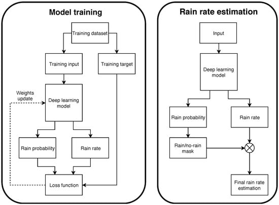
Figure 2.
Flowchart for the training phase of the model (left) and its use to estimate precipitation rate after training (right).
In the following section, we will describe in more detail how the data is prepared before being fed to our model and how we split the data in a training, a validation and a test set. Then, we will present the architecture of our model and its training strategy.
3.1. Model Inputs
Our convolutional model requires input data on a Euclidean grid. The chosen grid is the equal area satellite grid described in Section 2, on which we interpolated the satellite data and resampled the rain gauge data. All the different inputs are used to form a multi-spectral image that will be fed to our model, with each input corresponding to a different channel (Table 1).

Table 1.
List of all input channels, with their modality and timestamp. t corresponds to the time at which the model is making an estimation of the precipitation rates.
For the rain gauges channel, each rain gauge measurement is placed on the pixel located closest to the gauge and empty pixels are set to 0. For the network to be able to differentiate rain rate measurements of 0 to empty pixels, an additional channel is added with the rain gauge locations information. This channel is set to 0 everywhere except for pixels where the rain gauge measurements exist, which are set to 1 (Figure 3).
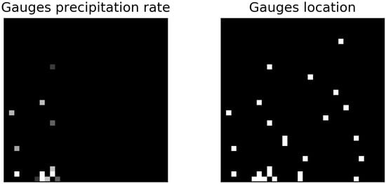
Figure 3.
An example of some of rain gauges channels used as input. The left channel alone renders pixels with rain gauges measurements of 0 indistinguishable from pixels lacking rain gauges measurements. The right channel allows for making this distinction by indicating the locations of the rain gauges measurements.
Although the three infrared satellite channels (8.7, 10.8, and 12.0 μm) were chosen to be useable under all illumination conditions, there may be some systematic variations of these inputs due to the diurnal or seasonal surface temperature variation. Therefore, we also included temporal information in one channel giving the time of the day and in another one giving the time of the year, in the form of periodical variables. For this, we take the cosinus of the temporal value, after conversion into radian. More explicitly, for the time of the day variable, 00:00 and 24:00 corresponds respectively to 0 and 2π rad; while for the time of the year variable, 01/01-00:00 and 12/31-24:00 corresponds to 0 and 2π rad, respectively. Since topography also has an influence on the weather, we also included the ground elevation as one of the input channels. Finally, because the weather is highly dependent to the situation 15 min in the past, we added the satellite and rain gauges measurements from the previous timestamp (Table 1). We also expect these additional measurements to increase our model’s robustness to the measurement errors, coming from either the measurement devices themselves or the temporal interpolation made for the rain gauges measurements during the data preparation. The reason we added past information directly as input, instead of using recurrent networks as the Long Short-Term Memory or the Gated Recurrent Unit cells [19,20], is because we are not doing any forecasting, making the use of long time series unnecessary for the purpose of our study.
3.2. Data Splitting
For an accurate performance evaluation, a proper data splitting into a training, a validation and a test set is required. For this purpose, different rain gauges must be assigned to each set which was done using ratios of 80% (training)/10% (validation)/10% (test). Instead of assigning the gauges randomly to each set, leading to a sub-optimal spatial coverage for each different set, we picked the test and validation gauges using probabilities depending on their relative distances (Figure 4).

Figure 4.
Location for the training, validation and test automatic rain gauges.
Equivalently, it is important to split correctly in time the data to evaluate the performance on new meteorological events, unseen during training. The types and frequency of meteorological events depend of the season and may also depend of the year itself, so we want our validation and test sets to cover all seasons and years uniformly. For this, we built a ”validation-test set“ by taking all the dates in a year of 365 days and give them an index i, ranging between 1 and 365 (so date (1) is the 1st of January and date (365) is the 31th of December). We then pick all these dates from the year given by the equation: . Our “validation-test set" is then composed of 2016/01/01, 2017/01/02, 2018/01/03, 2016/01/04, etc., until y/12/31 (in this case, y is 2017). The “validation-test set" thus contains one year of composite data containing one third of the full 3-year 2016—2018 dataset. The remaining two thirds of the data are used for training. From the “validation-test set”, one day out of two is assigned to the validation set and the other to the test set. This choice of data splitting allows for each set to cover the three years of available data while minimizing the correlation between each set and keeps complete days for the test set—a necessity to evaluate the ability of our model to estimate daily rainfall using the RMIB’s climatological network of manual rain gauges. The Table 2 reviews the main statistics about the different datasets.

Table 2.
The fraction of non-null precipitation events and the mean and standard deviation for the non-null precipitation rate measurements of the training, validation and test set.
3.3. Model Architecture
Our problem is very similar to semantic segmentation applications where the aim is to assign each pixel from an image to a category. For example, the HSN model in [15] was trained to detect vegetation, buildings, vehicles and roads in high resolution aerial images. HSN is a convolutional neural network able to perform a multiscale analysis of its input and reached state-of-the-art performance on semantic segmentation for multi-channel aerial images. For these reasons, our model follows a similar encoder–decoder architecture (Figure 5). The proposed model can be split-up in three parts: an encoder, a decoder and two task-specific sub-networks. The encoder progressively reduces the resolution of the input through its maxpooling layers, allowing the convolutional kernels in the next layers to increase their spatial coverage. For example, during the first layer of the encoder, a 3 × 3 convolutional kernel covers a surface of 9 × 9 km2 and, after the first maxpooling layer, the resolution will be reduced by a factor 2 and the 3 × 3 kernels will be covering 18 × 18 km2. Additionally, to increase even more the multiscale transformation abilities of the model, inception layers [21] (Figure 6, Table 3) are used. These layers are made of different convolutional layers simultaneously performing their transformation at different kernel sizes. After the third maxpooling layer, the decoder progressively increases back the resolution by following a similar pattern as the encoder and using transposed convolution instead of maxpooling layers. As with the HSN architecture, we used residual modules (Figure 7) to transfer pre-maxpooling information back to the decoder, by concatenating the residual module output with the transposed convolution output. In this manner, we allow the model to recover the highest resolution details, which were lost during the successive maxpooling layers. Finally, at the end of the decoder, two sub-networks output respectively the probability of precipitation and the rain rate r in mm/h. Indeed, instead of training one different model for each task, we trained one multi-task model capable of outputting both the classification and regression results at once. This approach is justified because a network able to estimate the rain rate r should also be able to estimate . Additionally to the training time saving given by a single multi-task model, the performance of each separated task can improve and outperform the single-task models [16].
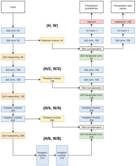
Figure 5.
Diagram of the proposed model architecture. Each convolutional layer is followed by a batch-normalization layer [22] and the ReLU activation function, except for the last 1 × 1 convolutional layers of each sub-networks. The output of the residual modules and the transposed convolutions are concatenated before being fed to the next layer.
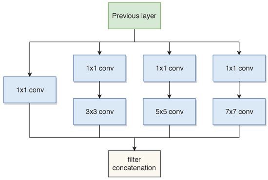
Figure 6.
Diagram of the inception module. The number of filters used for each layer is given in Table 3.

Table 3.
The number of filters for each type of convolution in the Inception modules. The “n × n reduce“ stands for the 1 × 1 convolutions preceding the concording n × n convolutions.
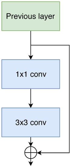
Figure 7.
Diagram of the residual module. The number of filters for the 1 × 1 layer and the 3 × 3 layer is the same, e.g., 64 for the top residual module appearing in Figure 4.
3.4. Training Strategy
To train the model, we built a dataset of all rain gauge measurements from the training set with and an equal amount of measurements with selected randomly. In a similar way, we built a validation set from the validation gauges and validation timestamps for hyper-parameter tuning.
As input, during training and validation, the model is fed with a patch of 32 × 32 pixels (covering 96 × 96 km2) centered on the rain gauge measurement taken as target coming from the training or validation dataset. In this patch, the rain gauges channels include data from all the rain gauges (i.e., from the training, the validation and the test set), except for the gauge used as target.
For each sample, the model performs both a classification and a regression by estimating and r from which we compute the binary cross-entropy loss and the mean squared error loss respectively. The mean squared error loss being only relevant for positive rain rate values, we set it to 0 for the samples with a null target rain rate; that way, the part of the model estimating the precipitation amount is only learning from the rainy training samples. To train our multi-task model, we must combine the different tasks losses into a single one, which is usually done by choosing a linear combination between them such as:
The problem with this approach is the addition of new hyper-parameters that are to be tuned manually to scale properly the different losses and to maximize each task’s performance. Instead of such manual tuning, we applied the method from [16] which considers the homoscedastic uncertainty of each task to allow the combination of the different losses as:
The parameters and in (2) are learnable and automatically optimized during the training of the model using the back-propagation algorithm. By using the same model weights for different tasks, multi-task learning can have a regularization effect. In our experience, this regularization effect proved to be sufficient and no additional regularization (as weight decay or dropout) was necessary (the validation loss drops until convergence after a similar number of epochs than the training loss, as is illustrated in Figure 8).
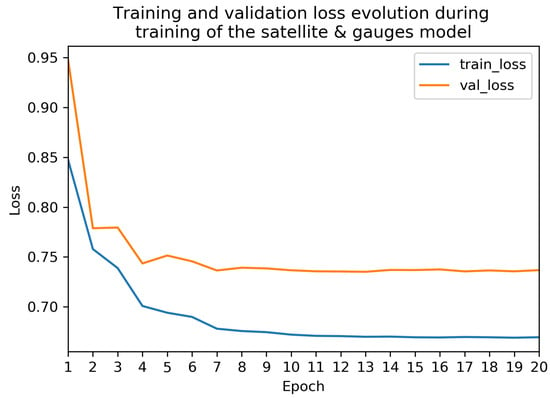
Figure 8.
The evolution of the training and validation loss during the training of the model.
A particularity of our training method is that, for each sample, the loss is computed in one single pixel due to the sparsity of the rain gauges used as training targets while it is usually computed on all pixels of the predicted image for semantic segmentation problems. Due to this restriction, when we trained the model by placing the targeted rain gauge measurement always on the same pixel location, i.e., in the center of the patch, the model estimation images suffered from a gridding effect. This problem was corrected by applying a random translation to the patch around the targeted pixel, allowing training of the model on different pixel locations.
Finally, the model was trained using a batch size of 128 and the Adam optimizer with a starting learning rate of divided by 5 every 2 epochs and using early stopping. The training was done on one RTX 2080 Ti using the library PyTorch. Our model started to converge after about 8 epochs (Figure 8), with each epoch taking approximately 2 h.
4. Results
4.1. Evaluation Method
We evaluated the ability of our model to detect precipitation and to accurately estimate their rate by computing various scores already used in previous studies [9,10]. The considered classification scores include the Probability Of Detection (POD), the False Alarm Ratio (FAR), the Probability of False Detection (POFD), the Accuracy (ACC), the Critical Success Index (CSI), the Gilbert Skill Score (GSS), the Heidke Skill Score (HSS), the Hanssen–Kuipers Discriminant (HKD) and the F1 score (F1). All these classification scores (Table 4) are computed from the contingency table made from the observations of the rain gauges and the estimations of our model (Table 5). For the regression scores (Table 6), we used the Mean Error (ME), the Mean Absolute Error (MAE), the Root Mean Squared Error (RMSE), the Reduction of Variance (RV), the Pearson Correlation Coefficient (PCORR) and the Spearman Rank Correlation (SCORR). Descriptive information about these scores is available in [10]. In the results section, all these scores were computed individually for each test gauge and then all of them were averaged.

Table 4.
The classification scores equation, value range and optimum value. The F1 score is calculated from the precision P and the recall R.

Table 5.
Contingency table between the observations and the estimations, recording the number of true negatives , the number of false negatives , the number of false positives and the number of true positives .

Table 6.
The regression scores equation, value range and optimum value. is an observation and is its estimation. The Spearman rank correlation is the Pearson correlation of the rank of the observations and the estimations.
For the evaluation of instantaneous precipitation, we computed the classification and regression scores on the test gauge measurements from the test timestamps, without balancing the dataset (i.e., using all measurements). The estimation was made using as input only the rain gauge measurements from the training and the validation gauges. The model was trained on 32 × 32 pixels patches but, for the evaluation on the test set, we could use as input the complete area of our study by taking a patch of 360 × 352 pixels (fitting very easily in the memory of a single RTX 2080 ti), thus making the estimations for all the test gauges at once. For comparison, we also trained two additional models, one without the rain gauges as input (called the satellite model) and one without the satellite as input (called the gauges model), allowing quantification of the contribution of each modality to the performance of the multimodal model (also called the satellite and gauges model, in the following section). As a reference point, we also compared the performance of our model to a geostatistical interpolation method of rain gauges. For that, we use ORdinary Kriging (ORK) with a linear variogram model, using the 20 closest measurements, to reduce computation time, at a very limited cost in performance. This method was used in [12], where a comparison was made between different radar-gauge merging methods and the ORK interpolation of rain gauges. More complex climatological variograms (i.e., Gaussian, exponential and spherical) have been tested in [12] but without any significant observed performance improvement, which is consistent with the results in [23].
4.2. Instantaneous Precipitation Detection Evaluation
From the rain probability estimation of our model, we distinguish precipitating pixels from those not precipitating by using a probability threshold of above which pixels are considered to be rainy: . The most straightforward choice of decision boundary would be to use , but, due to the different distribution in rain/no-rain events encountered during training (as explained in the training strategy, we balance the training dataset) compared to the real distribution, will predict too much precipitation events. Instead, we have to treat as an additional hyper-parameter that we optimize by maximizing the F1 score on the validation data (Figure 9).
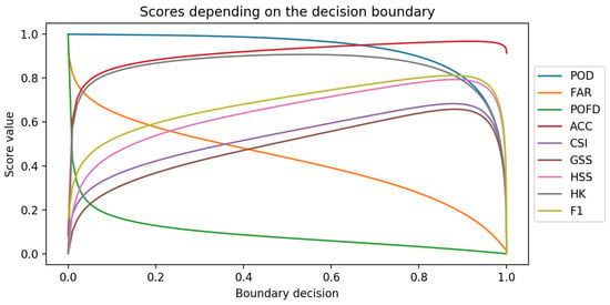
Figure 9.
Classification scores vs boundary decision for the satellite and gauges model, computed on the training and validation data.
ORK is not suited for instantaneous precipitation detection and is expected to give a very high False Alarm Rate, rendering the comparison of ORK rain detection performance with our models rather useless. For this reason, we developed a rain detection ORK method by applying a rain rate threshold under which every ORK estimation are set to zero. The rain rate threshold is optimized on the validation gauges.
From the results in Table 7, we can see that when used alone, the rain gauges modality is much better than the satellite modality for precipitation detection. The ratio POD/FAR is particularly better for the gauges model and the CSI, GSS, HSS, HKD and F1 metrics, which are less dependent to the classes frequency than the ACC, bring the same conclusion. Despite this clear domination of the rain gauges modality, the satellite and gauges model obtain better results than gauges only, proving the benefits of our multimodal approach. When comparing the multimodal model to the gauges model, the POD is slightly lower but the FAR and POFD get a net improvement. These results are in line with our expectations. Indeed, the rain gauges offer us direct precipitation measurements, but their spatial sparsity decreases their ability to detect precipitations occurring on a small area (typical of convective precipitations) and their ability to detect accurately the precipitation area limits. Adding the three infrared satellite channels allows for detecting precipitation in an indirect way but with a higher spatial resolution and reduces the shortcoming of the rain gauges modality stemming from their spatial sparsity. Our multimodal model and our gauges model is performing better than the reference kriging method. The fact that the gauges model is outperforming the kriging estimation imply that our model is particularly suited for rain detection.

Table 7.
Classification scores computed on the test set, for the model using both modalities (Satellite and gauges), the model using only the rain gauges (Gauges) the model using only the satellite channels (Satellite) and ordinary kriging using a precipitation detection threshold (ORK with threshold) and without applying any threshold (ORK).
4.3. Instantaneous Precipitation Rate Evaluation
For the evaluation of the precipitation rate estimation, we compute the regression scores only on precipitating events, because the precipitation detection part of our model is already taking care of non-precipitating events by setting them to zero and we want here to evaluate only the precipitation rate estimation part of our model. For this reason, the regression scores were computed using only the test measurements with (Table 8). Again, we expect the gauges model to perform better than the satellite model. The PCORR and SCORR corroborates this expectation but, very surprisingly, the MAE and the RMSE scores are better for the satellite model than for the gauges model. A possible explanation would be that the satellite model is better fitted to estimate high precipitation rate, coming from convective precipitations, and which are occurring on smaller areas, something harder for the gauges model to estimate.

Table 8.
Regression scores averaged on the automatic test stations. The ME, the MAE and the RMSE are expressed in mm/h.
The multimodal model is clearly benefiting from both modalities and outperforms the single modality models as well as the kriging interpolation of the rain gauges. On the other hand, the fact that our gauges model results are worse compared to those of the kriging interpolation lets us believe that there is room for improvements.
4.4. Visual Evaluation for Instantaneous Precipitation Estimation
For an additional qualitative evaluation, we perform a visual inspection of the estimations of our models, and compare them to the interpolation of rain gauges with kriging (with and without thresholding) and to the Belgian radar composite made by RMIB. First, we would like to point out that due to the restricted window size during the training, the estimations of the gauges model are unconstrained on areas without any rain gauge measurements (see training and validation gauges location in Figure 2). Secondly, due to the limited range of the radars, the Belgian radar composite is obviously not able to detect precipitations too far away from Belgium. Thirdly, radar QPE has some limitations to detect light rain. In [2], the radar QPE does not detect rain rates lower than 0.1 mm/h.
Our first example shows a winter precipitation case (Figure 10). The gauges model gives an acceptable estimation of the precipitations near the Belgium/Germany border but is completely unable to make any relevant estimation for the North of France and the North Sea. We can see the effect of some of the KNMI’s rain gauges near the Netherlands coast, but their sparsity is too high to render them useful. For the satellite model, the general shape of the precipitation map is very similar to the one of the radar image and of the satellite and gauges model, but the number of false alarm is very high, showing its limitation to discriminate very low precipitation rate areas from non-precipitating areas. With the help of both modalities, the precipitation estimation of the satellite and gauges model is getting very close to the radar composite. Remarkably, it can detect some of the precipitations outside of the area covered by the rain gauges while keeping the number of false alarms much lower than the satellite model, when we take the radar image as a reference. Comparing our multimodal model to the kriging interpolation of the rain gauges gives another evidence of the added value of the satellite information. Some precipitation areas in the Netherlands and the North of France appearing in the radar are recovered by our multimodal model, but are completely missed by the rain gauge methods. This shows that our multimodal method performs well in areas with a low density of rain gauges.
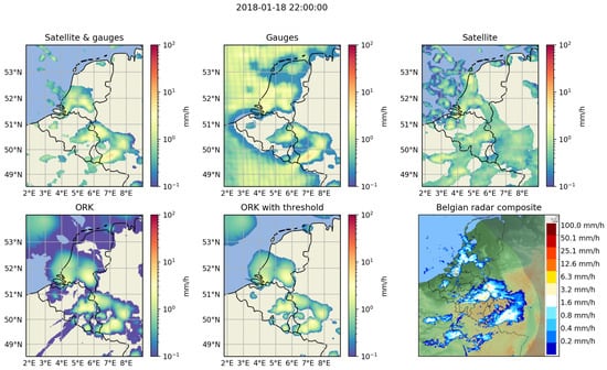
Figure 10.
Winter precipitation study case.
The next example is a case of convective precipitations during summer (Figure 11). An inspection of the different precipitation images from this figure gives a very similar conclusion to that drawn from the previous example. The satellite model seems to give less false alarms than for the winter case, but is still able to detect most of the strong precipitation areas. Thanks to the satellite, the multimodal model can detect much better the precipitations in the Netherlands, where the rain gauges are much sparser than in Belgium. We can also see that the multimodal model and the satellite model are able to detect a precipitation area in the top of the images that the radars are unable to detect because of their limited range. The kriging estimation, even with the precipitation threshold, is spreading precipitation everywhere on the map, in contrast to our ML models. When looking at Belgium, even our gauges model can delimit precipitation area quite well compared to the kriging estimates.
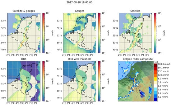
Figure 11.
Summer precipitation study case.
4.5. Daily Precipitations
Our model was additionally tested on the RMIB’s climatological network of rain gauges. This network consists of more than 250 rain gauges reporting the daily rainfall quantity across Belgium. Daily precipitation has much less spatial variability than instantaneous precipitation, making this evaluation method much more robust to data noise than the evaluation of the instantaneous precipitation rate estimation against automatic rain gauges done previously.
To reduce the spatial correlation between the gauges used as input (the automatic rain gauges from the training/validation set) and the climatological gauges used for evaluation, we kept only the climatological rain gauges located at least 3 km away from the closest automatic rain gauge of the training/validation set. We also excluded climatological gauges lacking measurements on the test days, leaving us with a total of 138 climatological rain gauges for the evaluation (Figure 12).
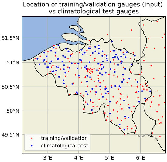
Figure 12.
Location of training and validation automatic rain gauges (used as input) and climatological rain gauges (used for evaluation), in Belgium.
To compute the daily precipitation quantity (in mm) from our model’s precipitation rate estimations (in mm/h), we averaged all instantaneous precipitation rate estimations of each test days for which there is no missing data (154 days out of the 182 test days are complete) and multiplied them by 24 h. As a reference, we compute the daily precipitation estimation from the kriging interpolation of the automatic rain gauges in a similar fashion. The detection scores (Table 9) and the regression scores (Table 10) have been computed on all available data. We have also separated the test days in two hydrological seasons, winter and summer, in order to evaluate the difference in performance between these two seasons (Table 11 and Table 12).

Table 9.
Daily precipitation detection scores averaged on the climatological test gauges, for the test days.

Table 10.
Daily precipitation regression scores averaged on the climatological test gauges, for the test days. The ME, the MAE and the RMSE are expressed in mm.

Table 11.
Daily precipitation detection scores averaged on the climatological test gauges, for the test days and separating the year into two hydrological seasons. The summer season starts on the 1st of April and finishes on the 30th of September.

Table 12.
Daily precipitation regression scores averaged on the climatological test gauges, for the test days and separating the year into two hydrological seasons. The summer season starts on the 1st of April and finishes on the 30th of September. The ME, the MAE and the RMSE are expressed in mm.
Our multimodal model performs the best for the daily precipitation detection (Table 9). The results of the gauges model come in a very close second. This is evidence that for daily precipitation estimation, the spatial variability of the precipitation field can be small enough to be accurately estimated from a dense network of rain gauges. Quite surprisingly, the satellite model performs also remarkably well, even surpassing by a large margin the kriging results. Stratiform precipitating clouds, typical of winter precipitation events, have less spatial variability than summer convective precipitating clouds. For this reason, we expect precipitation detection results to be better in the winter than in the summer, which is corroborated by the results of the rain gauges interpolation with the kriging method (Table 11). Surprisingly, the inter seasonal results difference is very small for the multimodal and the gauges models while the satellite model shows greater seasonal variability in its results.
As previously seen in the evaluation of instantaneous rain rate estimation, the results for daily precipitation quantity estimation in Table 10 shows that our model benefits from the merging of the satellite and rain gauges information. Unlike the results of Table 8, the satellite model performs rather poorly compared to the gauge modality, which means that the poor performance stems from its bad precipitation detection performance (Table 7 and Table 11). While our models were outperforming the kriging results for the precipitation detection, the kriging method shows slightly better performance for estimating daily precipitation quantity on all test days (Table 10). When looking at the seasonal results (Table 12), we see that our multimodal model performs best in the summer, confirming that satellite information improves precipitation estimation for convective rain.
5. Discussion
Compared to previous ML studies [4,9,10], we have introduced a multiscale, multimodal and multi-task DL model for precipitation area detection and instantaneous rain rate estimation from geostationary satellite imagery and rain gauges.
In Section 4, we compared the performance of our multimodal model against each modality used individually and the kriging interpolation rain gauge data, for instantaneous precipitation rate estimation and total daily precipitation estimation. The results allowed us to assess the strengths and weaknesses of each modality as well as the ability of our multimodal model to benefit from the combination of the two modalities, and outperform the kriging results for instantaneous precipitation rate estimation.
The rain gauges model provides good precipitation estimates where the density of the rain gauges network is high enough (e.g., in Belgium) but may still fail to catch very local precipitation events, typical of convective rains. If the rain gauges are too sparse, the precipitation estimates from rain gauges alone becomes very poor (e.g., in the Netherlands). Its performance is also lower compared to the kriging interpolation, indicating that further work should be considered to improve the integration of the rain gauge information into the DL model. For example, NN applied to point cloud data should be considered [24].
The main difficulty of the satellite model is to distinguish non-precipitating clouds from those with a very low precipitation rate. On the other hand, this modality does not suffer as much as the rain gauges modality from spatial variation in its performance due to local in situ measurements dependence and is also better at recovering small precipitating clouds.
By combining each modality, our multimodal model can avoid the shortcomings of each modality and combine their strengths. The rain gauges allow the multimodal model to improve the accuracy of the precipitation rate estimation and to better distinguish low precipitation clouds from those not raining, while the satellite strongly improves the estimation in areas with a very sparse rain gauges network and detects the small precipitating clouds missed by the rain gauges.
When looking at the performance for daily precipitation quantity retrieval in the summer, our model performs better than the rain gauges interpolation results obtained from the ordinary kriging interpolation of the rain gauges. However, the results of our model in the winter are worse compared to those obtained with the kriging interpolation of the rain gauges. This difference in the results between the winter and the summer confirms that the satellite modality has difficulty to treat low precipitation from stratiform rains but is an added value for convective rain. Also, for the precipitating area detection task at the daily scale, our model is performing much better than the kriging interpolation of the rain gauges.
The performance of our model is not only coming from its multimodality, but is also due to our careful choice of DL architecture. Indeed, where other studies used a shallow fully connected NN [4,10], we used a deep multiscale convolutional NN able to learn spatial dependence in its input at different scales.
Another novelty of our model is its multi-task aspect, giving an additional performance enhancement and allowing us to use a single model for both tasks, i.e., precipitation detection and precipitation rate estimation. This lies in contrast to previous ML studies [9,10] which used two different models for each task.
The results presented in this paper motivate further research in the application of DL to precipitation estimation. For example, one could restrict the model to only use the satellite modality and explore the benefits of using additional satellite channels, to obtain a global precipitation estimation from the complete geostationary window of MSG. Also, further work could be done on the multimodality aspect of our study, the radar being the obvious choice for the next modality to use.
6. Conclusions
In this study, we demonstrated the effectiveness of Deep Learning (DL) for multimodal rain rate estimation. For this purpose, we took advantage of state-of-the-art semantic segmentation techniques from DL and multi-task learning to develop a DL model able to estimate instantaneous rain rate from GEO satellite radiometer scans and automatic rain gauges measurements. Compared to existing rain gauges interpolation techniques and previous methods for rainfall retrieval from satellite radiometer data, our model can efficiently combine both modalities and to reduce each of their own individual downsides. More specifically, the rain gauges, which are the most direct devices for rainfall measurements, allow our model to recover accurate rain rate values while the satellite infrared channels improve the spatial resolution of the estimation and recover the small convective precipitations patches missed by the rain gauges because of their spatial sparsity.
Using automatic rain gauges for comparison, our multimodal model detects precipitation areas with a POD of 0.745, a FAR of 0.295 and a CSI of 0.564. It also estimates precipitation amount with a MAE of 0.605 mm/h and a RMSE of 1.625 mm/h for instantaneous rates.
Our model’s ability to efficiently combine different modalities and its promising results motivates further research in the application of cutting-edge DL techniques for Quantitative Precipitation Estimation (QPE).
Author Contributions
S.D. had the initial idea for the study while A.M. (Adrian Munteanu) proposed the multimodal approach and A.M. (Arthur Moraux) brought the multi-task aspect. A.M. (Adrian Munteanu) proposed the main architecture of the model which was further refined by A.M. (Arthur Moraux). A.M. (Arthur Moraux) developed the learning strategy, the software implementation and wrote the article. S.D., B.C. and A.M. (Adrian Munteanu) revised and commented the article.
Funding
This research was funded by the Royal Meteorological Institute of Belgium and the Solar Terrestrial Center of Excellence.
Acknowledgments
We would like to thanks all the external organizations providing us the data used in this study, i.e., EUMETSAT for the SEVIRI data, and Société bruxelloise de Gestion de l’Eau (SBGE), Vlaamse Milieumaatschappij (VMM), Service d’Etude Hydrologique (SETHY), the Koninklijk Nederlands Meteorologisch Instituut (KNMI) and the Deutscher Wetterdienst (DWD) for the automatic rain gauges data.
Conflicts of Interest
The authors declare no conflict of interest.
Abbreviations
General abbreviations:
| QPE | Quantitative Precipitation Estimation |
| GEO | Geostationary Earth Orbiting |
| RF | Random Forest |
| ML | Machine Learning |
| NN | Neural Network |
| DL | Deep Learning |
| ORK | ORdinary Kriging |
| MSG | Meteosat Second Generation |
| SEVIRI | Spinning Enhanced VIsible and InfraRed Image |
| HSN | Hourglass-Shape Network |
| BT | Brightness Temperature |
| RMIB | Royal Meteorological Institute of Belgium |
Scores abbreviations:
| POD | Probability Of Detection |
| FAR | False Alarm Ratio |
| POFD | Probability Of False Detection |
| ACC | Accuracy |
| CSI | Critical Success Index |
| GSS | Gilbert Skill Score |
| HSS | Heidke Skill Score |
| HKD | Hanssen–Kuipers Discriminant |
| F1 | F1 score |
| ME | Mean Error |
| MAE | Mean Absolute Error |
| RMSE | Root Mean Squared Error |
| RV | Reduction of Variance |
| PCORR | Pearson Correlation |
| SCORR | Spearman Rank Correlation |
References
- Foresti, L.; Reyniers, M.; Seed, A.; Delobbe, L. Development and verification of a stochastic precipitation nowcasting system for urban hydrology in Belgium. Hydrol. Earth Syst. Sci. 2016, 20, 505–527. [Google Scholar] [CrossRef]
- Goudenhoofdt, E.; Delobbe, L. Generation and Verification of Rainfall Estimates from 10-Yr Volumetric Weather Radar Measurements. J. Hydrometeor 2016, 17, 1223–1242. [Google Scholar] [CrossRef]
- Kidd, C.; Kniveton, D. R.; Todd, M. C.; Bellerby, T. J. Satellite rainfall estimation using combined passive microwave and infrared algorithms. J. Hydrometeorol. 2003, 4, 1088–1104. [Google Scholar] [CrossRef]
- Nguyen, P.; Ombadi, M.; Sorooshian, S.; Hsu, K.; AghaKouchak, A.; Braithwaite, D.; Ashouri, H.; Thorstensen, A.R. The PERSIANN family of global satellite precipitation data: A review and evaluation of products. Hydrol. Earth Syst. Sci. 2018, 22, 5801–5816. [Google Scholar] [CrossRef]
- Kidd, C. Satellite rainfall climatology: A review. Int. J. Climatol. 2001, 21, 1041–1066. [Google Scholar] [CrossRef]
- Rosenfeld, D.; Lensky, I. M. Satellite-Satellite-based insights into precipitation formation processes in continental and maritime convective clouds. Bull. Am. Meteorol. Soc. 1998, 79, 2457–2476. [Google Scholar] [CrossRef]
- Lensky, I. M.; Rosenfeld, D. Clouds-aerosols-precipitation satellite analysis tool (CAPSAT). Atmos. Chem. Phys. 2008, 8, 6739–6753. [Google Scholar] [CrossRef]
- Roebeling, R. A.; Holleman, I. SEVIRI rainfall retrieval and validation using weather radar observations. J. Geophys. Res. Atmos. 2009, 114. [Google Scholar] [CrossRef]
- Kühnlein, M.; Appelhans, T.; Thies, B.; Nauß, T. Precipitation estimates from MSG SEVIRI daytime, nighttime, and twilight data with random forests. J. Appl. Meteorol. Climatol. 2014, 53, 2457–2480. [Google Scholar] [CrossRef]
- Beusch, L.; Foresti, L.; Gabella, M.; Hamann, U. Satellite-Based Rainfall Retrieval: From Generalized Linear Models to Artificial Neural Networks. Remote Sens. 2018, 10, 939. [Google Scholar] [CrossRef]
- LeCun, Y.; Bengio, Y.; Hinton, G. Deep learning. Nature 2015, 521, 436. [Google Scholar] [CrossRef] [PubMed]
- Goudenhoofdt, E.; Delobbe, L. Evaluation of radar-gauge merging methods for quantitative precipitation estimates. Hydrol. Earth Syst. Sci. 2009, 13, 195–203. [Google Scholar] [CrossRef]
- Schmetz, J.; Pili, P.; Tjemkes, S.; Just, D.; Kerkmann, J.; Rota, S.; Ratier, A. An introduction to Meteosat second generation (MSG). Bull. Am. Meteorol. Soc. 2002, 83, 977–992. [Google Scholar] [CrossRef]
- Goovaerts, P. Geostatistics for Natural Resources Evaluation; Oxford University Press: New York, NY, USA, 1997. [Google Scholar]
- Liu, Y.; Minh Nguyen, D.; Deligiannis, N.; Ding, W.; Munteanu, A. Hourglass-shapenetwork based semantic segmentation for high resolution aerial imagery. Remote Sens. 2017, 9, 522. [Google Scholar] [CrossRef]
- Kendall, A.; Gal, Y.; Cipolla, R. Multi-task learning using uncertainty to weigh losses for scene geometry and semantics. In Proceedings of the IEEE Conference on Computer Vision and Pattern Recognition, Salt Lake City, UT, USA, 18–23 June 2018; 7482; 7491. [Google Scholar]
- Chen, R.; Li, Z.; Kuligowski, R. J.; Ferraro, R.; Weng, F. A study of warm rain detection using A-Train satellite data. Geophys. Res. Lett. 2011, 38. [Google Scholar] [CrossRef]
- Alfeld, P. A trivariate clough—Tocher scheme for tetrahedral data. Comput. Aided Geom. Des. 1984, 1, 169–181. [Google Scholar] [CrossRef]
- Xingjian, S.H.I.; Chen, Z.; Wang, H.; Yeung, D.Y.; Wong, W.K.; Woo, W.C. Convolutional LSTM network: A machine learning approach for precipitation nowcasting. In Proceedings of the Neural Information Processing Systems, Montréal, QC, Canada, 7–12 December 2015; pp. 802–810. [Google Scholar]
- Shi, X.; Gao, Z.; Lausen, L.; Wang, H.; Yeung, D. Y.; Wong, W. K.; Woo, W. C. Deep learning for precipitation nowcasting: A benchmark and a new model. In Proceedings of the Neural Information Processing Systems, Long Beach, CA, USA, 4–9 December 2017; pp. 5617–5627. [Google Scholar]
- Szegedy, C.; Liu, W.; Jia, Y.; Sermanet, P.; Reed, S.; Anguelov, D.; Erhan, D.; Vanhoucke, V.; Rabinovich, A. Going deeper with convolutions. In Proceedings of the IEEE conference on computer vision and pattern recognition, Boston, MA, USA, 7–12 June 2015; pp. 1–9. [Google Scholar]
- Ioffe, S.; Szegedy, C. Batch normalization: Accelerating deep network training by reducing internal covariate shift. In Proceedings of the 32nd International Conference on Machine Learning, Lille, France, 6–11 July 2015; pp. 448–456. [Google Scholar]
- Haberlandt, U. Geostatistical interpolation of hourly precipitation from rain gauges and radar for a large-scale extreme rainfall event. J. Hydrol. 2007, 332, 144–157. [Google Scholar] [CrossRef]
- Bronstein, M. M.; Bruna, J.; LeCun, Y.; Szlam, A.; Vandergheynst, P. Geometric deep learning: Going beyond euclidean data. IEEE Signal Process. Mag. 2017, 34, 18–42. [Google Scholar] [CrossRef]
© 2019 by the authors. Licensee MDPI, Basel, Switzerland. This article is an open access article distributed under the terms and conditions of the Creative Commons Attribution (CC BY) license (http://creativecommons.org/licenses/by/4.0/).