Article

Spatial Resolution Matching of Microwave Radiometer Data with Convolutional Neural Network

1
Beijing Key Laboratory of Millimeter Wave and Terahertz Technology, Beijing Institute of Technology, Beijing 100081, China
2
Shenzhen Institutes of Advanced Technology, Chinese Academy of Sciences, Shenzhen 518000, China
3
Department of Electronic Engineering, Tsinghua University, Beijing 100084, China
4
Faculty of Electrical Engineering, Delft University of Technology, 2600 GA Delft, The Netherlands
*
Author to whom correspondence should be addressed.
Remote Sens. 2019, 11(20), 2432; https://doi.org/10.3390/rs11202432
Submission received: 24 September 2019 / Revised: 16 October 2019 / Accepted: 17 October 2019 / Published: 19 October 2019
(This article belongs to the Special Issue Image Super-Resolution in Remote Sensing)

Abstract

:
Passive multi-frequency microwave remote sensing is often plagued with the problems of low- and non-uniform spatial resolution. In order to adaptively enhance and match the spatial resolution, an accommodative spatial resolution matching (ASRM) framework, composed of the flexible degradation model, the deep residual convolutional neural network (CNN), and the adaptive feature modification (AdaFM) layers, is proposed in this paper. More specifically, a flexible degradation model, based on the imaging process of the microwave radiometer, is firstly proposed to generate suitable datasets for various levels of matching tasks. Secondly, a deep residual CNN is introduced to jointly learn the complicated degradation factors of the data, so that the resolution can be matched up to fixed levels with state of the art quality. Finally, the AdaFM layers are added to the network in order to handle arbitrary and continuous resolution matching problems between a start and an end level. Both the simulated and the microwave radiation imager (MWRI) data from the Fengyun-3C (FY-3C) satellite have been used to demonstrate the validity and the effectiveness of the method.

Graphical Abstract

1. Introduction

Satellite based remote sensing with microwave radiometers has been widely used in observing unique microwave emission features from earth [1]. It has the advantages of continuously measuring large area both day and night and under most weather conditions [2]. Many atmospheric and surface parameters, such as precipitation rate, cloud liquid water, and sea ice concentration, etc., can be retrieved through these observations [3]. However, these retrievals are often hampered by the problem of non-uniform spatial resolution, when multi-frequency observations must be combined, leading to low resolution and even estimation errors of the retrievals [4,5,6]. To alleviate this problem, the obvious solution is to average the high frequency channel, which has the higher spatial resolution, to match down to the low frequency channel. But it is not desirable when geophysical parameters, such as rainfall, are highly nonlinear with the radiances, or the retrieval parameters are used in regional-scale studies [5,6,7]. Therefore, it is preferable to increase the spatial resolution of the low frequency channel to match up with the high frequency channel.
In order to enhance the spatial resolution of the microwave radiometer data, several degradation factors should be reduced, including the antenna pattern, the integration time, the scan geometry, and the receiver sensitivity. Specifically, due to the limited size and long working distance of the satellite antenna, the observed data are smoothed by the wide beam width of the antenna pattern, leading to the low spatial resolution [6,7,8,9,10,11]. Secondly, considering the integration time of the radiometer, the equivalent antenna pattern is further broadened [12]. Moreover, the relative geometry of the observation changes along with the conical scan, which makes the resolution spatial variable [8,9,10,11]. Lastly, the receiver sensitivity of the radiometer leads to the noise of the observation [3,10,11].
Traditionally, many analytic algorithms have been proposed to ease these degradation factors so as to raise the spatial resolution. The Backus–Gilbert (BG) method and the Wiener filtering method are both direct inverse-based methods. The BG method utilizes the redundant overlapping footprint information to reconstruct a smaller equivalent antenna pattern, thus the spatial resolution can be improved [10,12,13]. This method has also been extensively used to match the resolution of different frequency channels [4,5,6]. The Wiener filtering method restores the image with space variant filters in the frequency domain in order to reduce the degradation caused by the antenna pattern and the scan geometry change [9,14]. The scatterometer image-reconstruction (SIR) algorithm and the reconstruction method in Banach space (Banach method) are all iterative gradient methods, and the degradation factors are included in matrix A of the general problem form: Ax=b. The SIR method solves the inverse problem in Hilbert space [10] whereas the Banach method in Banach space [15], which leads to the reduction of the over-smoothing effect and oscillation due to the Gibbs phenomenon. However, all these analytic methods are suppressed by rapid noise amplification. Thus, the resolution enhancing and matching ability is limited.
Recently, learning-based methods have also been used for microwave radiometer data spatial resolution enhancement [11,16,17], which directly learn an end-to-end mapping between low- and high-resolution images. Due to the powerful mapping ability of the convolutional neural network (CNN) on image restoration problems and the efficient training implements on modern GPUs [18,19], complicated degradation factors can be comprehensively learned during the training process. Thus, these methods achieve better enhancement results than the regularly used BG and Wiener methods [11,16,17]. However, the existing learning-based methods are now incompatible with the practical resolution match problem for the following reasons. Firstly, the learning pairs in the dataset do not match to the spatial resolution of actual working channels, leading to a mismatch between the learned enhancement level and the real task level. Secondly, during the retrieval of various meteorological parameters, different multi-frequency combinations should be considered, which leads to building a very large ‘model zoo’ when using supervised learning-based methods. For example, when retrieving global snow depth (SD) form the Fengyun-3C (FY-3C) microwave radiation imager (MWRI) observations, the 10.65, 18.7, and 36.5 GHz channel should be combined [4]. However, when retrieving the regional SD in China, the 10.65, 18.7, 36.5, and 89.0 GHz channel should be considered, thus the spatial resolution of these low frequency channels is better to match up to 89 GHz in this case [4,20]. Lastly, when cross-calibration and data fusion between similar satellite radiometer instruments (MWRI [3], Special Sensor Microwave/Imager (SSM/I) [9,10,21] and Advanced Microwave Scanning Radiometer-Earth Observing System (AMSR-E) [6], etc.) are considered [3,4,21,22], the spatial resolution should be matched to the same level, which makes the generation of the dataset more difficult and even unavailable.
In this paper, in order to solve these problems, a novel and practical microwave radiometer data accommodative spatial resolution match (ASRM) framework is proposed. Specifically, with the help of the modified degradation model to generate the adaptive datasets, the learning-based method is able to effectively match the spatial resolution of the low frequency channel to various discrete high frequency channels. Moreover, by simply tuning an input coefficient, the method can be adjusted to produce arbitrary and continuous resolution match results between the trained fixed levels without the extra training process. The illustration of the method is shown in Figure 1.
Overall, the contributions of this paper are as follows:
(i) A flexible degradation model, based on the imaging process of the microwave radiometer, is proposed to generate the datasets. Thus, for various levels of matching problems, large amounts of suitable learning pairs can be provided for training and testing of the network.
(ii) For the fixed level resolution match problems, utilizing the powerful mapping ability of the deep residual CNN, our network can more properly match the resolution to the corresponding high frequency channels than some state of the art methods while restraining the noise amplification.
(iii) The interactive adaptive feature modification (AdaFM) layers are added to the network in order to handle arbitrary resolution match problems. By simply adjusting an interpolation coefficient, the network could generate continuous and smooth resolution enhancement results without extra training processes.
The rest of this paper is organized as follows. Section 2 introduces the MWRI instrument and its imaging process. The resolution match method, including the degradation model, the network architecture, the framework flowchart, and the training details, is proposed in Section 3. Then, both the fixed level and the arbitrary level resolution match demonstrations are shown in Section 4. Finally, Section 5 and Section 6 draw the discussion and conclusion, respectively.

2. Instrument and Imaging Process

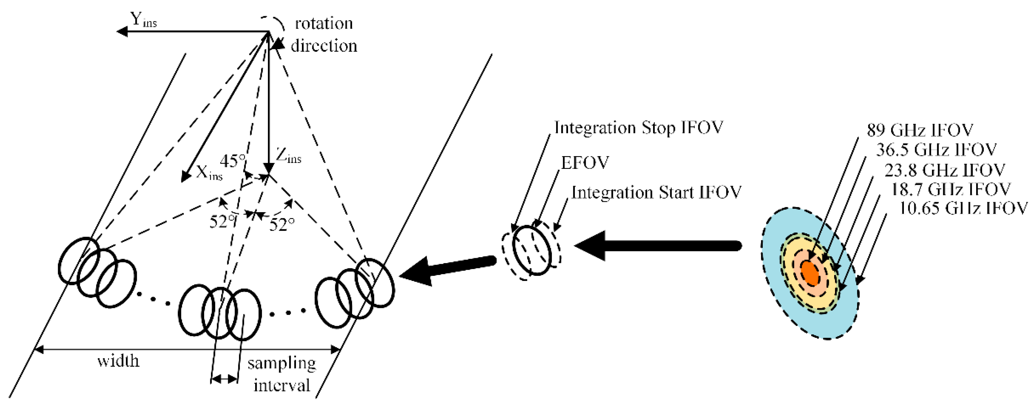
2.1. MWRI Instrument

The FY-3C is one of the Chinese FY series of meteorological polar-orbiting satellites [2]. The on-board MWRI is a total-power passive radiometer that measures the radiance at 10.65, 18.7, 23.8, 36.5, and 89.0 GHz with both vertical (V) and horizontal (H) polarizations. The emission energy from earth is collected by the main parabolic reflector of size 977.4 × 897.0 mm [8] and is then fed to different horns with different working frequencies. Therefore, due to the different electrical size of the antenna, the instantaneous field of view (IFOV) of different channels varies from 9 × 15 km @ 89.0 GHz to 51 × 85 km @ 10.65 GHz across and along the satellite track direction. Meanwhile, each observation sample is collected with the corresponding integration of time in order to reduce noise, as illustrated with the equivalent field of view (EFOV) in Figure 2 [3]. The specific performance of the FY-3C MWRI instrument is shown in Table 1 [8,22], where the NEΔT is the receiver sensitivity (noise equivalent differential temperature) [3].
The scan geometry illustration of the FY-3C MWRI is shown in Figure 2. The positive Xins axis shows the satellite heading direction while the positive Zins axis points downward to the satellite nadir point. The orbit height of the satellite is 836 km and the main reflector scans the earth conically with a viewing angle of θ = 45° and spinning rate of 1.8 s/rotation. The forward cone scanning method is adopted to cover a swath of 1400 km, completing a measurement area within ±52° around the Zins axis. With the sampling interval of 2.08 ms, a total of 254 earth observation samples are obtained in each scanning rotation. And each image file of 254 × 1725 pixels is collected by 1725 continuous conical scans. The Level-1 (L1) data (http://satellite.nsmc.org.cn/portalsite/default.aspx) acquired by the FY-3C MWRI are used for the demonstration and validation in this paper.

2.2. Imaging Process

The antenna collects microwave radiance from earth, which can be represented by [12]:
t A ( s 0 ( t 0 ) , v , p ) = 1 τ t 0 τ / 2 t 0 + τ / 2 [ 4 π t B ( s , v , p ) G ( s 0 ( t ) , s , v , p ) d Ω 4 π G ( s 0 ( t ) , s , v , p ) d Ω ] d t ,
where t A ( s 0 ( t 0 ) , v , p ) is the temperature information collected by the antenna at the given direction s0(t0), frequency v, and polarization p. t0 is the observation time and τ is the integration time. The t B ( s , v , p ) is the brightness temperature and G ( s 0 ( t ) , s , v , p ) is the gain function of the antenna. It is worth mentioning here that for the simplicity of the problem, some minor factors, such as the atmospheric effects and the milliseconds-level short-term change of the brightness temperature, are neglected. Furthermore, only the scaler version of the antenna temperature is considered, thus the antenna cross polarization and polarization mismatch between earth surface and antenna pattern are also excluded in this expression [23].
Normalizing the antenna gain function and omitting the argument p to simplify the notation, Equation (1) can be expressed by:
t A ( s 0 ( t 0 ) , v ) = 1 τ t 0 τ / 2 t 0 + τ / 2 [ 4 π t B ( s , v ) F ( s 0 ( t ) , s , v ) d Ω ] d t ,
where F ( s 0 ( t ) , s , v ) is the normalized antenna pattern, and changing the sequence of the time integration and the space integration, the antenna temperature can be expressed by:
t A ( s 0 ( t 0 ) , v ) = 4 π t B ( s , v ) F ¯ ( s 0 ( t 0 ) , s , v ) d Ω ,
where
F ¯ ( s 0 ( t 0 ) , s , v ) = 1 τ t 0 τ / 2 t 0 + τ / 2 F ( s 0 ( t ) , s , v ) d t ,
is the effective normalized antenna pattern, which considers the effect caused by the integrating process [12].
It should be noted that all the equations above are expressed in the antenna viewing axis coordinate system (AVA) [8] for ease of presentation. However, the majority of the image processing operations are done in image domain, where the observation data lie in rectangular grids regardless of the scan mode. Thus, the coordinates transformation from the AVA to the image domain should be incorporated [8]. Meanwhile, considering the sampling interval of the radiometer, the discrete temperature image collected by the antenna in image domain can be represented by:
t A ( x , y , v ) = x , y t B ( x , y , v ) h ( x , y , x , y , v ) ,
where t A ( x , y , v ) and t B ( x , y , v ) are the antenna temperature image and the brightness temperature image represented with row and column indexes in the image domain. h ( x , y , x , y , v ) , which is transformed from the effective normalized antenna pattern F ¯ ( s 0 ( t 0 ) , s , v ) in AVA, is the point-spread-function (PSF) ( x , y h ( x , y , x , y , v ) = 1 ) in the image domain [11]. It should be noted that, because of the conical scan geometry, the orientation and shape of the PSF change along with the scanning positions [8,9,11]. Thus, the regular simplification of regarding h ( x , y , x , y , v ) as space invariable and transforming the integration operation in Equation (5) to the convolution operation [5,9,14,16,17,24]:
t A ( x , y , v ) t B ( x , y , v ) h ( x , y , v ) = F 1 [ T B ( u , v , v ) H ( u , v , v ) ] ,
is excluded in this paper so as to improve the model accuracy. Where T B ( u , v , v ) and H ( u , v , v ) are the two-dimensional discrete Fourier transformation (2d-DFT) of t B ( x , y , v ) and h ( x , y , v ) , and F 1 [   ] is the inverse 2d-DFT operation.
When the receiver sensitivity is considered, the imaging process can be finally expressed by:
t A ( x , y , v ) = x , y t B ( x , y , v ) h ( x , y , x , y , v ) + n ( x , y , v ) .
Overall, with the consideration of these degradation factors, including the antenna pattern, the integration time, the scan mode, and the receiver sensitivity, the imaging process of the satellite radiometer is discussed. During the degradation procedure in Equation (7), the integration with the PSF drastically smooths the brightness temperature image, which lowers the spatial resolution to a great extent. The integrating process of the radiometer, which tends to broaden the PSF in the cross-track direction, further amplifies the smoothing effect. Moreover, because of the changing geometry, the shape and direction of the PSF change along with the conical scan, especially in the cross-track direction [11], which leads to resolution spatial variable. In addition, the imaging process is polluted by the receiver sensitivity. Therefore, methods should be taken to cope with these degradation factors so that the spatial resolution of the antenna temperature images can be improved to match up with the high frequency channels.

3. Spatial Resolution Match Method

To adaptively match the spatial resolution of the microwave radiometer data, an ASRM framework, composed of the flexible degradation model, the residual deep CNN, and the adjustable AdaFM layers, is proposed. Then, the training details of the method are introduced.

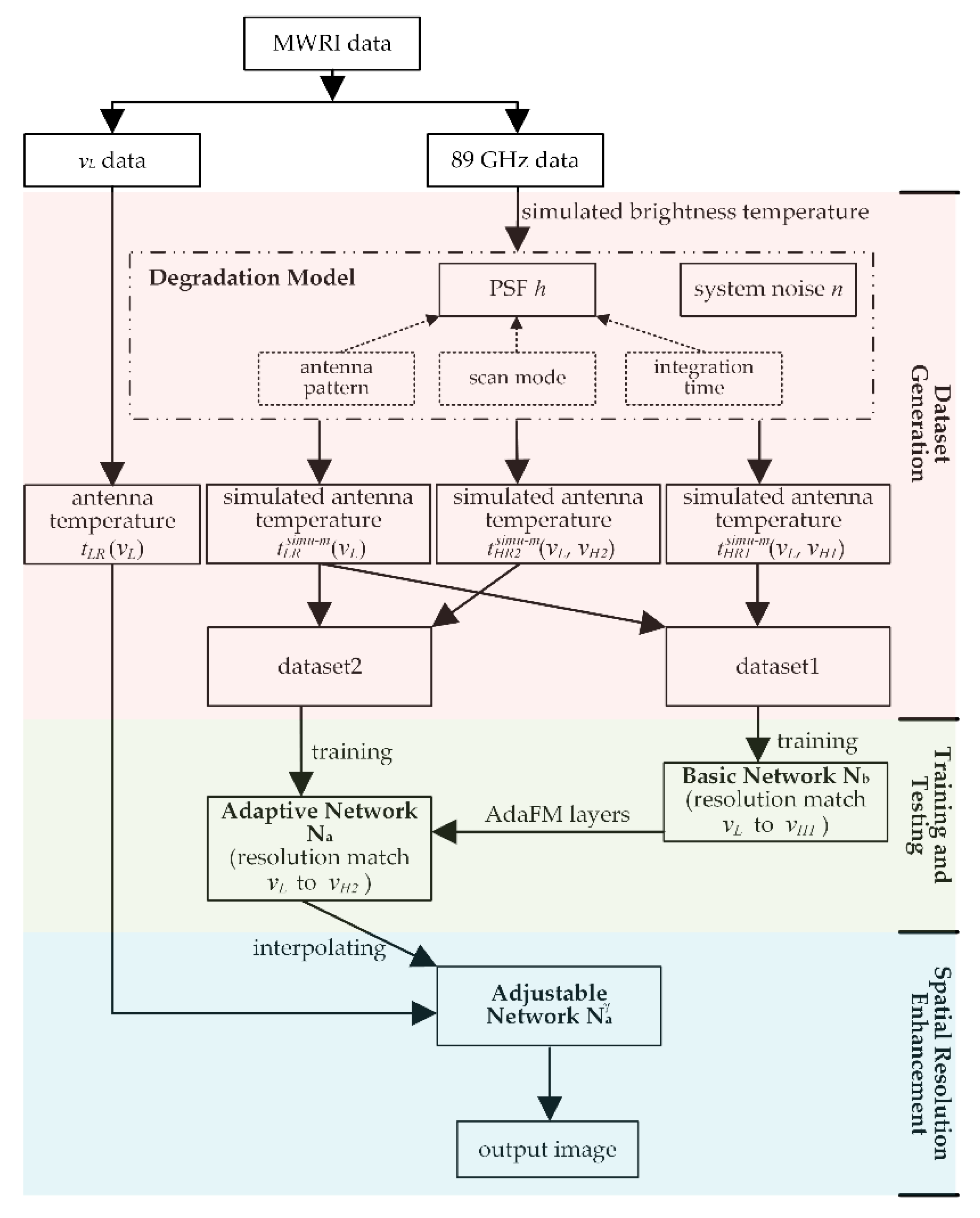
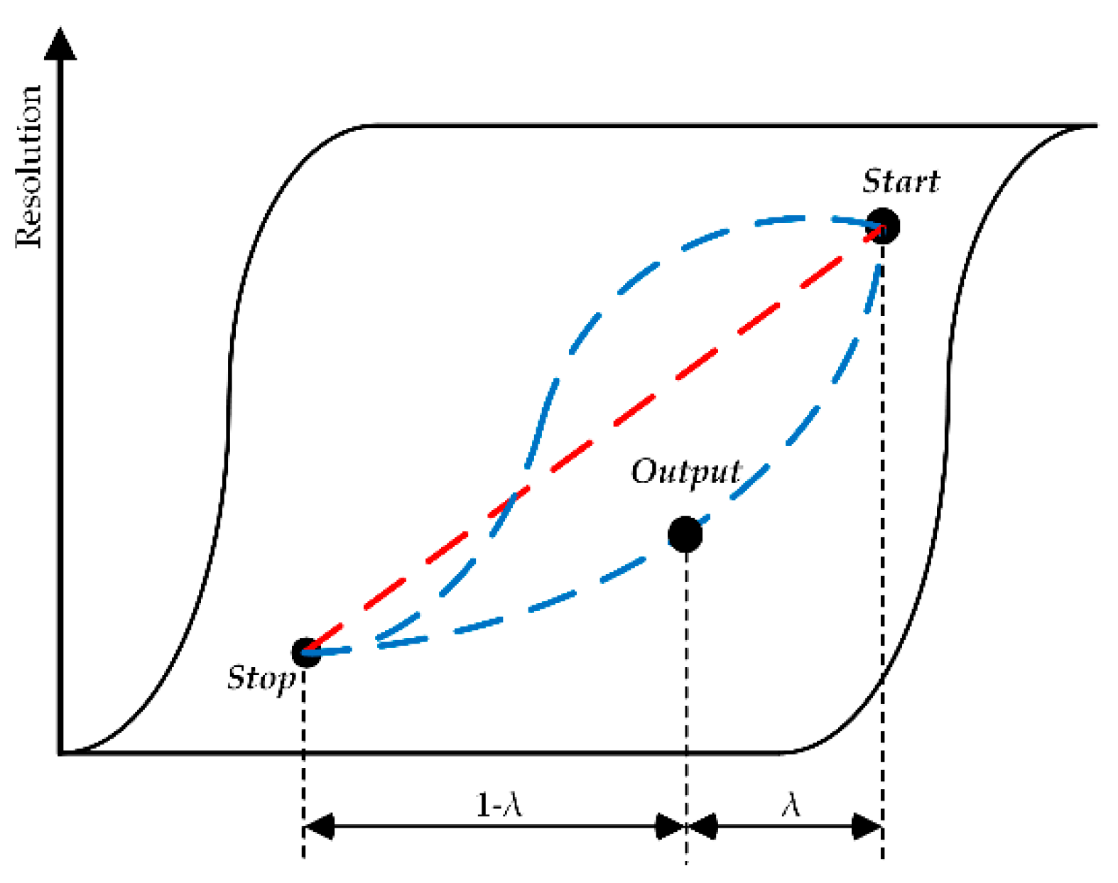
3.1. Flexible Degradation Model

The learning-based methods are often challenged by the difficulties of adaptively and effectively generating the dataset. Utilizing the characteristics of MWRI that multi-frequency bands scan the region in the exact same way and at the same time, several low resolution/high resolution (LR/HR) dataset generation methods were proposed [11,16,17]. However, these models are unfit for the real matching problems, leading to the domain adaptation problem (the label-rich data for training are unmatched with the label-scarce data for practical use). Thus, in this paper, we proposed a modified degradation model to generate the suitable image pairs for resolution matching. Furthermore, this model can be flexibly adjusted for various levels of matching tasks.
According to the imaging process (Equation (7)) that we discussed above, the ideal learning LR/HR image pairs for resolution match from low frequency channel v L to high frequency channel v H are expressed as:
t L R ( v L ) = t A ( x , y , v L ) = x , y t B ( x , y , v L ) h ( x , y , x , y , v L ) + n ( x , y , v L ) ,
t H R ( v L , v H ) = x , y t B ( x , y , v L ) h ( x , y , x , y , v H ) ,
where LR image t L R ( v L ) = t A ( x , y , v L ) is the actual observed data in the low frequency channel and t H R ( v L , v H ) is its ideal HR counterpart. For t H R ( v L , v H ) , as can be seen in Equation (9), the low frequency brightness temperature t B ( x , y , v L ) is equivalently observed by the noise-free high frequency v H manner (apart from the receiver sensitivity, the imaging process is the same with the actual v H channel). Thus, the spatial resolution of t H R ( v L , v H ) is the same with the v H channel. However, as the brightness temperature t B ( x , y , v L ) is unavailable, the ideal HR label cannot be realized.
Utilizing the image to frequency domain transformation, a LR/HR dataset was proposed [17], which can be shown as:
t L R s i m u 1 ( v L ) = F 1 [ T A ( u , v , v H ) H ( u , v , v H ) H ( u , v , v L ) + N ( u , v , v L ) ] F 1 [ T B ( u , v , v H ) H ( u , v , v L ) + N ( u , v , v H ) H ( u , v , v H ) H ( u , v , v L ) + N ( u , v , v L ) ] ,
t H R s i m u 1 ( v H ) = t A ( x , y , v H ) F 1 [ T B ( u , v , v H ) H ( u , v , v H ) + N ( u , v , v H ) ] ,
where T A ( u , v , v H ) , T B ( u , v , v H ) , H ( u , v , v H ) , H ( u , v , v L ) , N ( u , v , v H ) , and N ( u , v , v L ) are the 2d-DFT of t A ( x , y , v H ) , t B ( x , y , v H ) , h ( x , y , v H ) , h ( x , y , v L ) , n ( x , y , v H ) , and n ( x , y , v L ) , respectively. t L R s i m u 1 ( v L ) is the simulated v L data and t H R s i m u 1 ( v H ) is the real observed v H data. On the one hand, as we discussed in the imaging process, the simplification in Equation (6) neglected the changing geometry of the conical scan mode, which reduces the accuracy of this degradation model. On the other hand, during this LR/HR mapping, the noise might even be amplified ( N ( u , v , v H ) may be larger than N ( u , v , v H ) / H ( u , v , v H ) H ( u , v , v L ) + N ( u , v , v L ) in some cases). Therefore, the resolution matching effect is reduced, which will be demonstrate in Section 4.1.3.
Because the 89 GHz channel has the highest spatial resolution, it was used to make the simulated LR/HR datasets, which achieved good resolution enhancement results for the real measured data [11,16], as expressed by:
t L R s i m u 2 ( v 18 ) = x , y t A ( x , y , v 89 ) h ( x , y , x , y , v 18 ) + n ( x , y , v 18 ) ,
t H R s i m u 2 ( v 18 , v 89 ) = t A ( x , y , v 89 ) ,
where v 18 and v 89 represent 18.7 GHz and 89 GHz, respectively. It can be seen that the mapping learned from this image pair tries to eliminate the noise and the smoothing effect caused by PSF, thus it is effective in resolution enhancement and noise reduction. However, by comparing with the ideal learning pairs between Equations (8) and (9), we can find that the learned resolution enhancement level is higher than the practical matching demand when 18 GHz resolution is matching up to 89 GHz resolution. Thus, this dataset is mismatched with the real enhancement level.
Partially inspired by Gong. R. et al. [25], which have shown that the intermediate domains between the source and target domain (Equations (12) and (13) for this problem) are useful for addressing the domain adaptation problem, we produce several intermediate resolution levels to solve this mismatch problem and to accommodate different levels of resolution matching tasks.
Therefore, in order to generate an accommodative dataset for training and testing so that the learned mapping could be applied to the resolution match, we proposed a modified LR/HR image pair, which can be expressed as:
t L R s i m u m ( v L ) = x , y t A ( x , y , v 89 ) h ( x , y , x , y , v L ) + n ( x , y , v L ) ,
t H R s i m u m ( v L , v H ) = x , y t A ( x , y , v 89 ) h ( x , y , x , y , v H ) .
In terms of spatial resolution, the highest 89 GHz images have the most similar achievable features to the brightness temperature images. Thus, for the resolution matching problems in this paper, the 89 GHz data were also used as the simulated brightness temperature images, like in Hu. W. et al. [11,16]. As for the resolution match, the corresponding high frequency PSF h ( x , y , x , y , v H ) is added to act on the simulated brightness images, so that the resolution enhancement level can be matched to the real demand. Furthermore, based on the different levels of matching tasks, the parameters can be flexibly changed in this degradation model to manipulate the corresponding resolution enhancement level.
Then, the mapping function between the t L R s i m u m ( v L ) and t H R s i m u m ( v L , v H ) image pairs would be learned by CNN during the training process. After that, the spatial resolution of the low frequency channel v L could be matched up to the desired high frequency channel v H and the noise would be reduced at the same time.

3.2. Network Architecture

CNNs are feed-forward artificial neural networks [18]. In recent years, diverse CNNs have been proposed to solve optical image restoration problems (denoise [19,26], deblur [19,27], and super-resolution [18,26,28,29], etc.) and reach state of the art quality. Thus, in this paper, utilizing the powerful mapping ability of the CNN and the adjustable feature of the AdaFM layer, we have proposed an adjustable deep residual CNN to solve the adaptive resolution match problems.

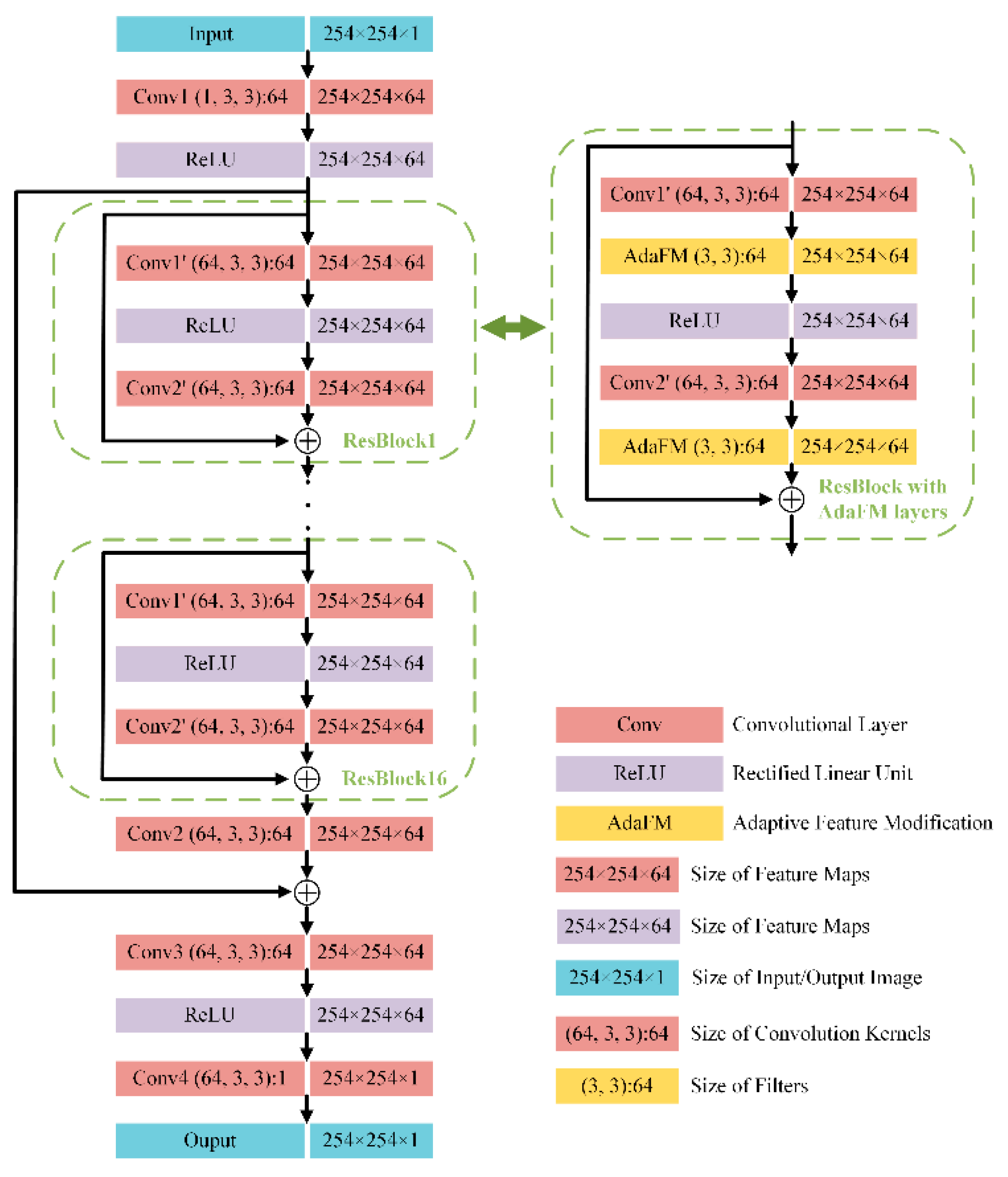
3.2.1. Basic Network

The goal of our resolution match problem is to train a restoring mapping function that reconstructs the HR image from its LR counterpart. During the training process, the network should jointly learn the complicated degradation factors and reduce the noise. Deep (large number of layers) CNNs spontaneously integrate more low/mid/high level features in a multilayer end-to-end fashion, thus they have more powerful mapping and feature extraction capacity [30], which is very suitable for our resolution enhancing problem.
However, normal deep plain-stacked CNNs usually face the problems of mapping degradation and gradient exploding/vanishing [31]. Therefore, residual learning has been introduced in deep CNNs to solve these obstacles. Instead of mapping H(X) by several plain-stacked layers, the residual learning explicitly lets these layers map the residual function F(X)=H(X)-X, and finally outputs F(X)+X with a shortcut connection from the input X. Although both methods should be able to asymptotically approach the same function, the ease of training could be different. With this residual learning technique, deep CNNs are easier to optimize and are able to get better results [26,28,29,31]. In addition, for our resolution enhancing problem, the LR images are the smoothed version of the HR images. In other words, the input of the network is quite similar to the label, only missing some high frequency components (gradient information). Thus, the shortcut connections in the network will help to speed up and improve the training process [17].
Therefore, in order to match the spatial resolution of different frequency channels, we introduced a deep residual CNN. The architecture of the network is show in Figure 3. All the network parameters Θ are optimized through the training process, where the differences (loss function) between the reconstructed images N b ( t L R s i m u m ( v L ) , Θ ) and the corresponding high-resolution images t H R s i m u m ( v L , v H ) are iteratively minimized. After that, the network can be used to deterministically match the resolution from channel v L to v H .

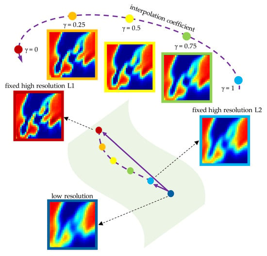
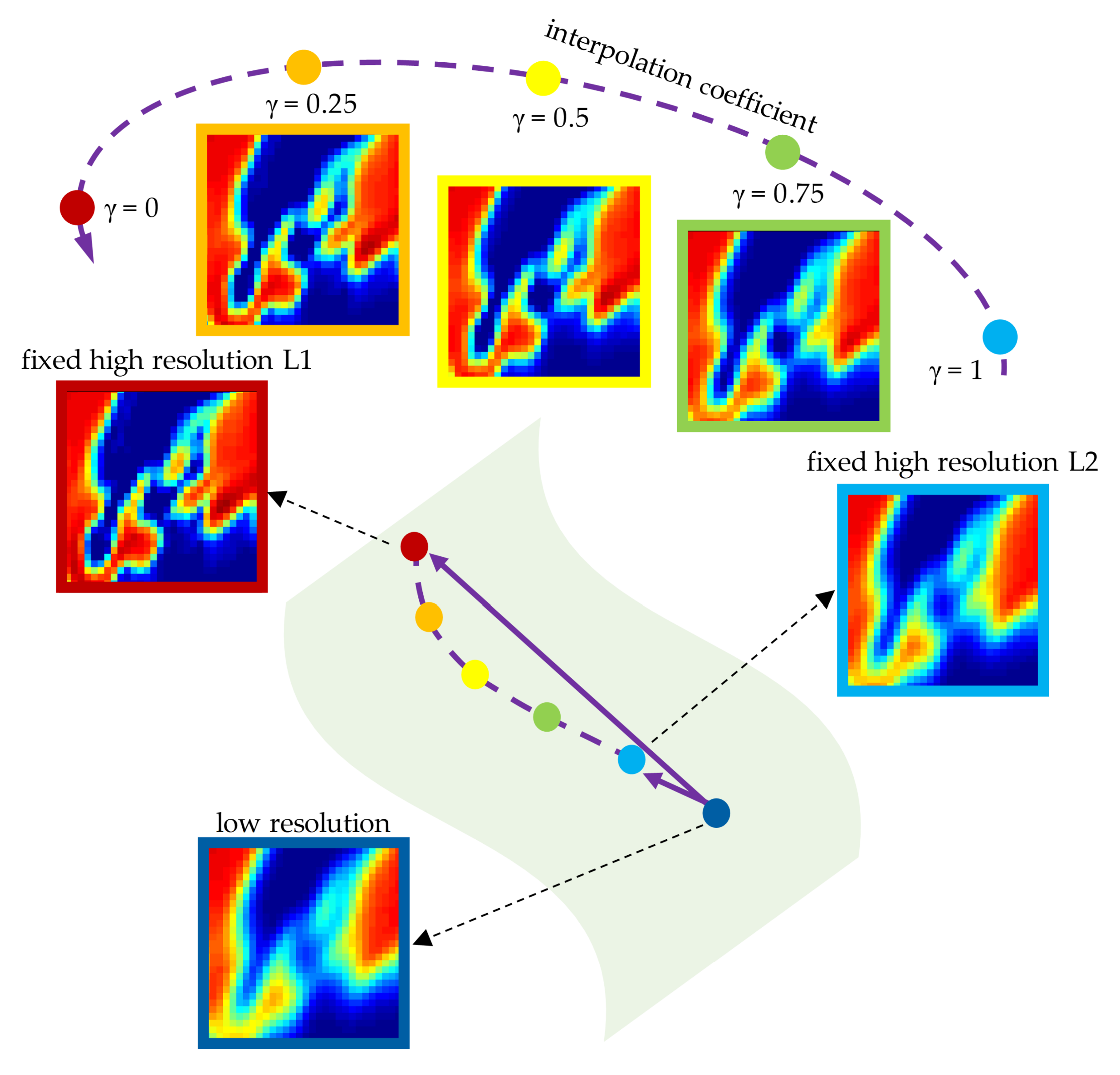
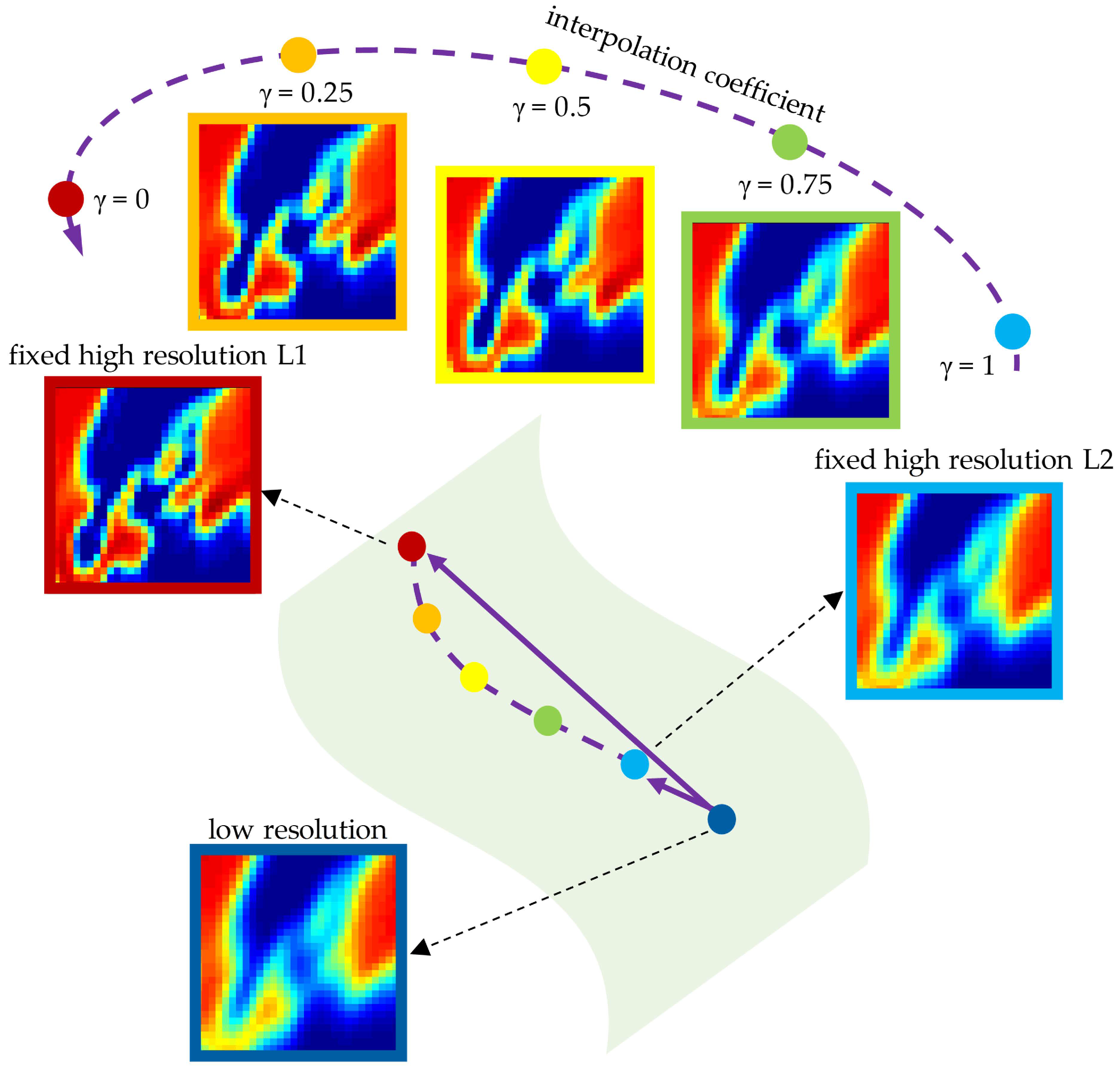
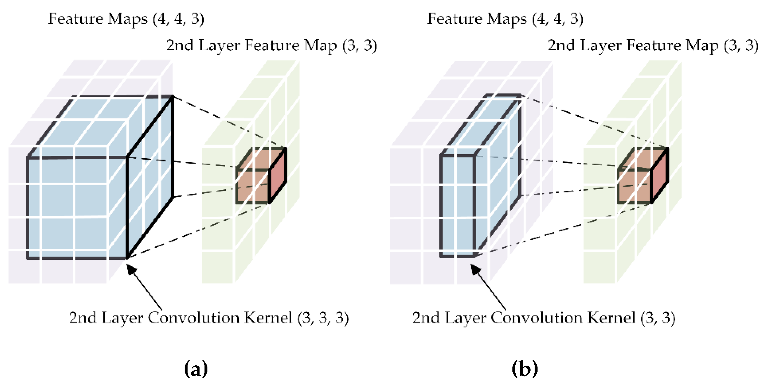
3.2.2. Adjustable Network

When cross-calibration or data fusion between several similar satellite radiometers are considered [3,4,21,22], the spatial resolution of the data should be matched to the same level. For example, when the cross-calibration between the FY-3C MWRI 18.7 GHz channel (30 × 50 km IFOV) and Aqua AMSR-E 18.7 GHz channel (16×27 km IFOV) is conducted, the spatial resolution of the MWRI 18.7 GHz channel is better to match up to its counterpart. However, the generation of direct learning image pairs between two different satellites is impracticable due to their different system parameters (viewing angle, scan geometry, bandwidth, etc.). Meanwhile, according to the discussion in Section 3.1, only fixed levels of resolution match is available (18 × 30 km [email protected] GHz or 9 × 15 km [email protected] GHz), and learning from discrete and fixed enhancement levels, the network cannot be easily and effectively generalized to other levels. Therefore, in this paper, methods are taken to generalize the network to arbitrary tasks between the fixed learned levels.
Inspired by the fact that CNN could be manipulated by the AdaFM layers to implement different denoise levels without extra training [26] and that customized intermediate products between different target domains can be linearly produced by simply adjusting an input coefficient [25], we introduced the AdaFM layers and the input coefficient to our network so as to smoothly adjust the resolution enhancement level.
The i th AdaFM layer is formulated as:
AdaFM i ( X ) = G i X + B i ,
where X are the input feature maps (m, m, nin), * denotes for the group convolution operation (the convolution operation works in two-dimensions instead of three [26], as shown in Figure 4b), and G i (f, f, nin) and B i (1, 1, nin) represent filters and biases, respectively. According to Equation (16), by inserting an AdaFM layer after a convolutional layer, each feature map output by the convolutional layer can be further adjusted. In other words, the statistics of the convolutional layer can be manipulated by the following AdaFM layer.
Our aim is to add these extra layers to the trained basic network Nb, so that the new network could be adapted to another enhancement level. Thus, by inserting an AdaFM layer after each convolutional layer in the ResBlocks, the adaptive network Na is created, as shown in Figure 3. The principle and the working process of the adjustable network N a λ are shown in the following steps:
Step 1: The basic network Nb that we discussed above is trained based on dataset1 ( t L R s i m u m ( v L ) and t H R 1 s i m u m ( v L , v H 1 ) ). So that the network Nb can deterministically match the resolution from v L to v H 1 .
Step 2: The AdaFM layers are inserted to the basic network Nb to form the adaptive network Na. By fixing all the parameters in the trained network Nb, only the parameters in the AdaFM layers are optimized according to dataset2 ( t L R s i m u m ( v L ) and t H R 2 s i m u m ( v L , v H 2 ) ) (the rationality of this training method is demonstrate in Section 4.2). Therefore, the adaptive network Na is transformed to match the resolution from v L to v H 2 .
Step 3: By interpolating the additional input coefficient λ, we can easily manipulate the parameters of the filters and biases in these AdaFM layers without additional training:
G i = I + λ ( G i I ) ,   B i = λ B , 0 < λ < 1 ,
where G i and B i are the interpolated filters and biases in these AdaFM layers. Thus, the relatedness of the network with different fixed enhancement levels can be accordingly adjusted.
So far, the adjustable network N a λ is created. Only by tweaking an interpolation coefficient λ, the network N a λ can generate arbitrary and continuous resolution enhancement results between a start ( v L to v H 1 ) and an end ( v L to v H 2 ) level.
However, the relationship between the coefficient λ and the resolution enhancement level may not be linear. As shown in Figure 5, it is assumed that there is a manifold of domain, where the images with the same spatial resolution can be seen as a point in the domain. Specifically, when λ = 0, the output images with v H 1 resolution can be seen as the point Start. And when λ = 1, the output images with v H 2 resolution can be seen as the point Stop. By tuning λ in the range of [0,1], we thus obtain a sequence of points flow from Start to Stop. But the path varies a lot according to the positions (resolutions) of the endpoints and the range between them, as illustration with the blue dash lines in Figure 5.
In order to explore the linear relationship (labeled with red dash line in Figure 5) between the interpolation coefficient and the resolution enhancement level, polynomial function λ = F ( R ) is fitted by M typical output points { R i , λ i } i = 0 M 1 in the test set, where R is the spatial resolution of the image. By linearly mapping the resolution to the range of [0,1]: R = M ( γ ) , Equation (17) can be modified to:
G i = I + T ( γ ) ( G i I ) ,   B i = T ( γ ) B , 0 < γ < 1 ,
where T ( γ ) = F ( M ( γ ) ) = λ .
As a result, the modified interpolation coefficient γ can be used to linearly and continuously manipulate the resolution enhancement levels of the adjustable network N a γ .

3.3. ASRM for the FY-3C MWRI

3.3.1. ASRM Framework Flowchart

The ASRM task for the satellite microwave radiometer data is implemented by a supervised adjustable CNN N a γ . The flowchart of the framework is shown in Figure 6 and the working process is introduced in the following steps:
Dataset generation: Utilizing the feature that multi-frequency bands of the MWRI scan the region in the exact same way, the 89 GHz antenna temperature image, which has the highest spatial resolution, is used as the simulated brightness temperature image. With the full consideration of the degradation factors for each channel, the simulated antenna temperature images of the v L channel and the simulated antenna temperature images with the corresponding resolution of the v H 2 channel and the v H 1 channel are produced by the flexible degradation model (Equations (14) and (15)). Then the dataset1 ( t L R s i m u m ( v L ) and t H R 1 s i m u m ( v L , v H 1 ) image pairs) and dataset2 ( t L R s i m u m ( v L ) and t H R 2 s i m u m ( v L , v H 2 ) image pairs) are made to train the networks.
Training and testing: Dataset1 is used to train and test for the basic deep residual network Nb. Then, by fixing all the parameters in the trained Nb, the adaptive network Na, with the inserted AdaFM layers, is trained and tested by dataset2.
Spatial resolution enhancement: Eventually, the adjustable network N a γ could be used to match the real v L channel data t L R ( v L ) to arbitrary spatial resolution from v H 2 to v H 1 .

3.3.2. Training Details

For training and testing, 437 antenna temperature images (254 × 1725) of the MWRI 89 GHz channel with horizontal polarization were used to generate the datasets. These images were acquired from 1 June 2018 to 5 July 2018, containing sufficient geographical features. For each dataset, based on the corresponding degradation model (Equations (14) and (15)), a total of 4370 cropped sub-image pairs (LR/HR pairs) (254 × 254) were generated. 200 sub-image pairs were randomly selected as the testing set, and the remaining 4170 sub-image pairs were used as the training set. It is worth mentioning that although we used fixed sub-image size in the training process to reduce memory burden, the network could be applied to arbitrary image size during testing and the final spatial resolution enhancement process.
The filter size was set to 3 for all the filters and convolution kernels, and the reflect padding technique was used for all the convolution operations to reduce the boundary effect. The feature size was set to 64, and all the shortcuts for residual learning were parameter free (direct connection) because of the constant dimension through the network, as shown in Figure 3. All the networks were trained with the adaptive moment estimation (ADAM) optimizer by setting the learning rate to 10-4.
Several evaluation metrics were introduced in this paper to assess the image quality from different perspectives. The peak signal-to-noise ratio (PSNR) is a mean-squared error (MSE) evaluation index, which is defined as the ratio between peak signal power to average noise power [32]. Structural similarity (SSIM) measures the similarity of structural information between the two images, which is a more visually pleasing metric than the PSNR [33,34]. For estimating the performance in terms of spatial resolution, equivalent instantaneous field of view (IFOV’) [11,24] was used, which is defined as I F O V = max f w h m { c o r r [ I o u t , ( I l a b e l P S F f w h m ) ] } . It is notable that the fwhm is the mean value of the along-track and cross-track IFOV: fwhm = 1/2 × (cross-track IFOV+ along-track IFOV).
Instead of using the dominant 2 (MSE) loss function to maximize the PSNR index, we used the 1 loss to get a better general result of the network, considering the PSNR, SSIM, and artifacts [29,33]. Meanwhile, the 1 loss function could provide better convergence.

4. Experiment Results

4.1. Quantitative and Qualitative Evaluation of Fixed Level Resolution Match

In this section, the fixed level resolution match by the basic deep residual network Nb is evaluated. For demonstration, the spatial resolution of the 18.7 GHz channel is matched to the highest 89 GHz channel. The other resolution match levels can also be similarly applied, but in order to save space, they are not listed here. Not only the testing set (in the dataset), but also a synthetic scenario and the real MWRI measured data (outside the dataset) are used to fully evaluate the fixed level resolution match ability. The analytic algorithms, including the widely used inverse-based BG method [10,12,13] and the iterative Banach method [15], are shown for contrast. In addition, the results learned by several benchmark CNNs, including the SRCNN [11,16,18] (3 layers, without the interpolation process), VDSR [28] (8 layers, without the interpolation process), and SRResNet [35] (16 ResBlocks, without the pixel shuffle layer), are also displayed as the comparison. It is noted that, for our resolution matching problem, the size of the HR output is the same as the LR input, thus the operations or layers that are used to increase the pixels for the image are excluded from these super-resolution CNNs in this paper.

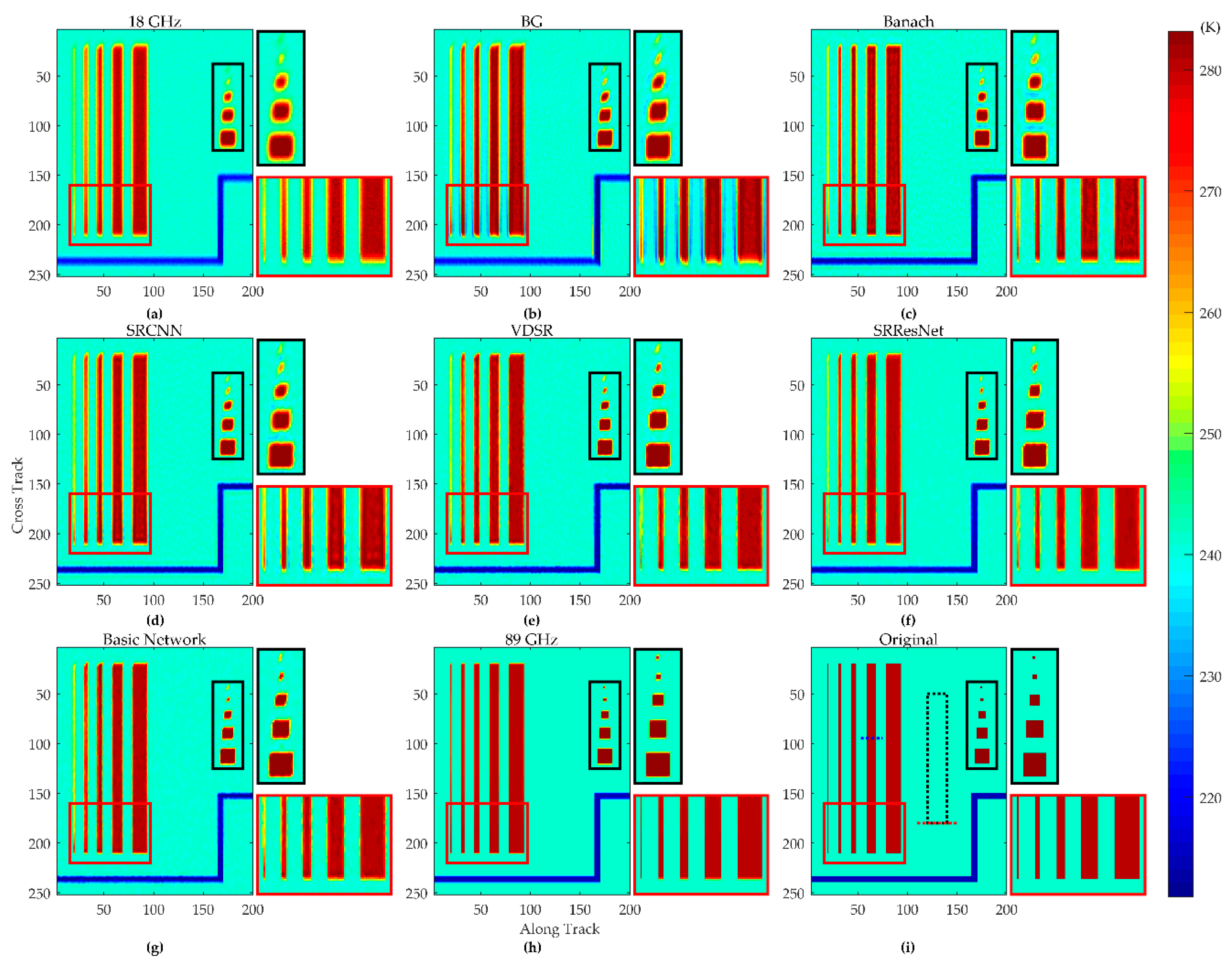
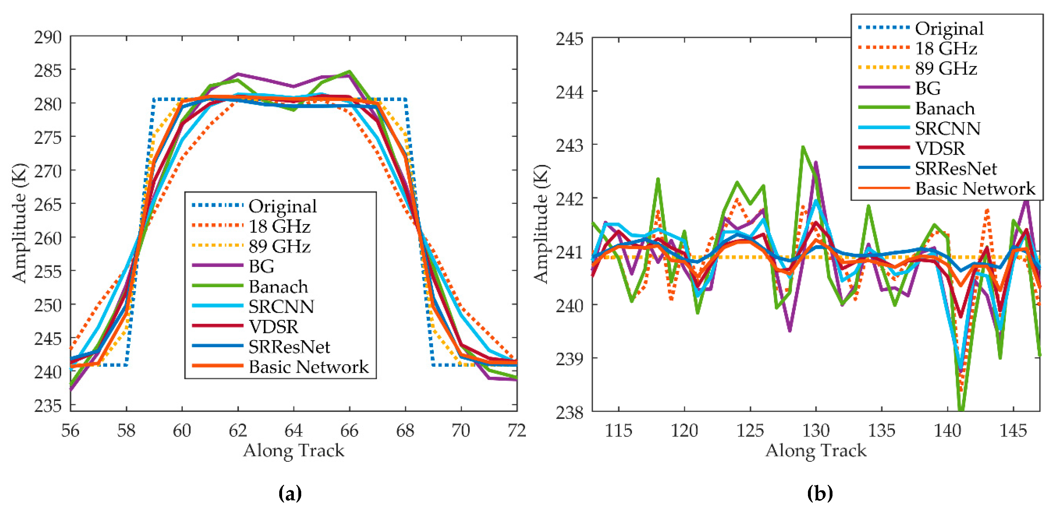
4.1.1. Synthetic Scenario Evaluation

Quantitative evaluation of the resolution enhanced image directly from the real MWRI data is inaccessible, since the response of different channels are diverse due to their frequency-dependent emissivity [5,7]. Synthetic data, however, offer an excellent substitute. Test data can be created from a known scene with the known noise, allowing for quantitative evaluations of the created methods.
The synthetic scenario, whose location information was the same as the MWRI data on 25 June, 2018 (top left and bottom right corner coordinates (Lat, Lon) were 7.6°N, 154.6°W, and 11.7°S, 172.3°W) is shown in Figure 7i. The synthetic scene consisted of 5 strips with 280.5 K amplitude, 190 pixels height, 10 pixels interval and 1, 3, 5, 10, and 15 pixels width; 5 square hot spots with 293.7 K amplitude, 10 pixels interval and 2, 3, 7, 11, and 15 pixels width; and a ‘river’ with 214.5 K amplitude and 6 pixels width. The amplitude of the background was 240.9 K, which is basically the same as the real 18.7 GHz data background. According to the imaging process, Figure 7a, h show the simulated 18.7 and 89 GHz antenna temperature images, respectively. It can be seen that, due to the different degradation parameters, the antenna temperature images were smoothed to different levels, and because of the conical scan geometry, the resolution was a spatial variable, as the narrowest strip shows in Figure 7. It should be mentioned that, in order to implement the evaluation of the resolution match effect and noise amplification level, the simulated 18.7 GHz antenna temperature was polluted with Gaussian white noise with the standard derivation of NEΔT (0.5 K for the 18.7 GHz channel, as shown in Table 1), whereas the 89 GHz antenna temperature was not.
Figure 7 also shows the match results of the synthetic scenario. The goal was to match the resolution of the 18.7 GHz channel to the 89 GHz channel. Figure 7b–g shows the results of the BG method, the Banach method, the SRCNN, the VDSR, the SRResNet, and the basic network Nb, respectively. The SRCNN, VDSR, SRResNet, and the basic network Nb were trained based on dataset1 ( t L R s i m u m ( 18.7 ) and t H R 1 s i m u m ( 18.7 , 89 ) image pairs). The local areas of the strips (enclosed by the red rectangle) and the square hot spots (enclosed by the black rectangle) are also enlarged for better visual evaluation.
As can be seen, our method produced very similar results to the 89 GHz channel. The hot spots were more focused and the boundaries of the strips were clearer. Furthermore, the learning-based methods tended to reduce the noise during the matching process, as can be seen on the strips in Figure 7.
In order to evaluate the results in a more intuitive way, Figure 8a shows the along-track transect (as labeled with the blue dash-dotted line in Figure 7i). As can be seen, the results of the basic network Nb were closer to the 89 GHz antenna temperature data than other methods and no notable artifact was introduced.
The resolution enhancement methods are often faced with the problem of noise amplification, so it is often a tradeoff between the resolution enhancement level and the noise amplification level [5,9,10,15]. However, by properly designing the learning image pairs, the network can reduce the noise while matching the spatial resolution. Figure 8b shows the along-track transect of the scenario (as marked with the red dash-dotted line in Figure 7i). As can be seen from the image, the learning-based methods effectively reduced the noise, whereas the inverse-based methods tended to amplify the noise. Independent experiments were done 100 times for statistical evaluation of the PSNR, SSIM, IFOV’, and the noise (standard variance of the data in the black dash-dotted area in Figure 7i). The averaged indexes are shown in Table 2, and the best indexes are shown in bold.
It should be noted that we created this synthetic scenario in order to intuitively evaluate the spatial resolution matching ability, the noise reduction ability, and the generalization performance of our basic network Nb. Because of the abrupt border, the synthetic scenario has sharper gradient features and higher frequency components than the simulated brightness temperature data, which are used to generate the dataset. Thus, the leaning-based methods suffered from some degrees of decline in terms of PSNR, SSIM, and IFOV’ (adaptation problem). Even so, the basic network Nb still outperformed the other methods.

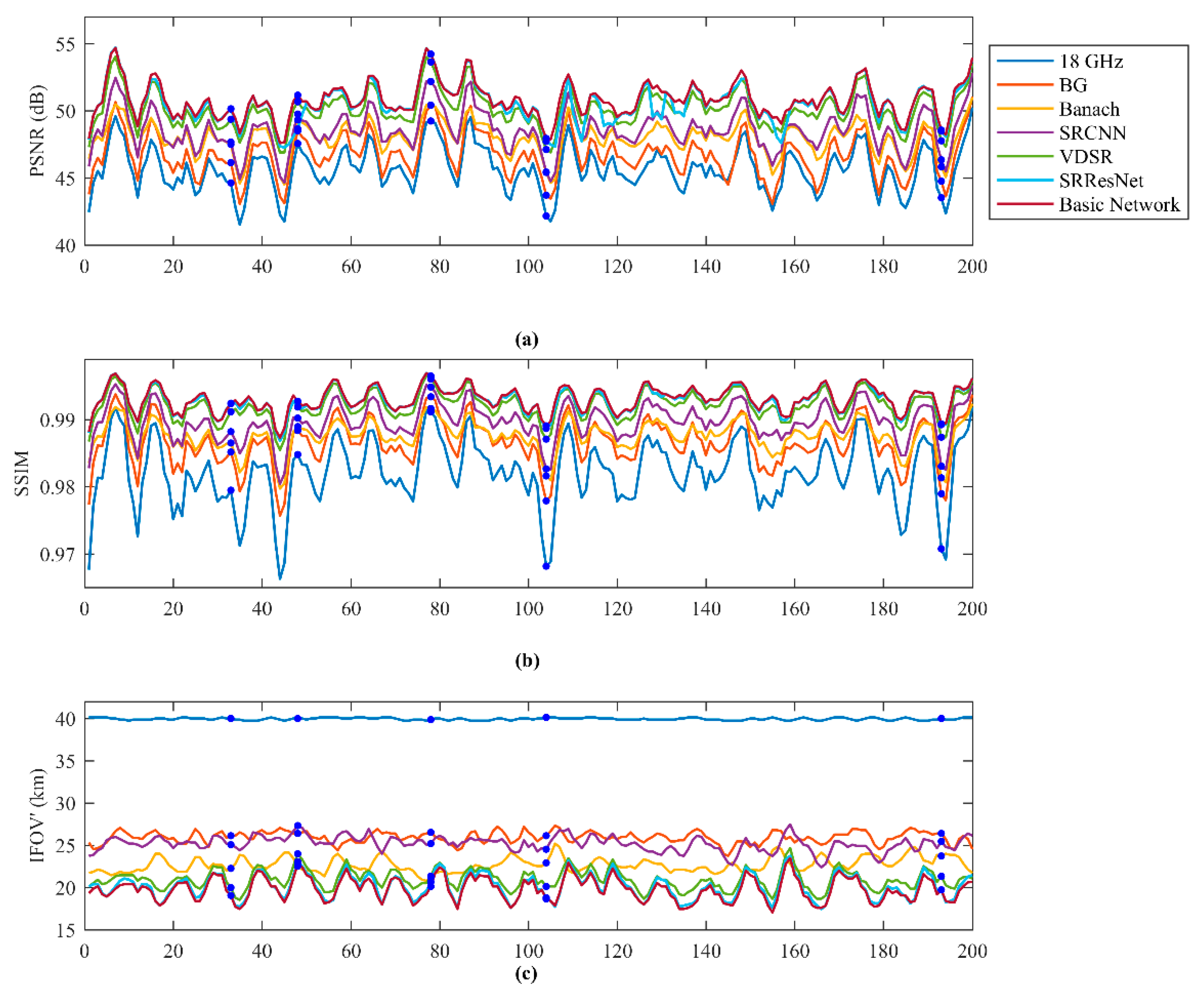
4.1.2. Test Set Evaluation

To further demonstrate the matching ability, the evaluations of all 200 images in the testing set are shown in Figure 9 (3 points smoothed for better presentation). The indexes of several typical scenes (marked with the blue points in Figure 9), and the averaged indexes of the whole testing set are shown in Table 3. Our method outperformed the other methods for all the testing images in terms of PSNR, SSMI, and IFOV’. The averaged PSNR of our method was 0.28 dB higher than the SRResNet, 0.68 dB higher than the VDSR, 2.23 dB higher than the SRCNN, 2.83 dB higher than the Banach method, and 4.12 dB higher than the BG method. The averaged SSIM is the same with the SRResNet and is improved by 0.001 compared with VDSR, 0.003 compared with SRCNN, 0.005 compared with the Banach method and 0.006 compared with the BG method. The IFOV’ of the basic network was 19.82 km, less than the SRResNet of 20.12 km, VDSR of 20.99 km, the Banach method of 22.70 km, SRCNN of 25.20 km, and the BG method of 25.94 km.
In order to present the comparison result visually, a typical scene around the Sea of Okhotsk, Russia (the 33th scene in the test set, as marked in Figure 9) is shown in Figure 10. The top left and bottom right corner coordinates of the scenario were 67.0°N, 170.3°E and 46.0°N, 127.4°E. This scene contained sufficient features of land, sea, bay, sea/land interface, and small islands, so that the performance of these methods could be comprehensively evaluated. The enlarged areas of the Bol’shoy Shantar island (enclosed by the black rectangle) and the northernmost part of the Sakhalin island (enclosed by the red rectangle) are shown in Figure 10. Our network could produce the clear boundaries and interfaces without noticeable artifacts. Furthermore, only through the basic network and SRResNet, the small island below the Sakhalin island could be distinguished, as shown in the black rectangle in Figure 10f,g. Either way, our method had the superior resolution match results with the simulated 89 GHz antenna temperature images in the testing set.

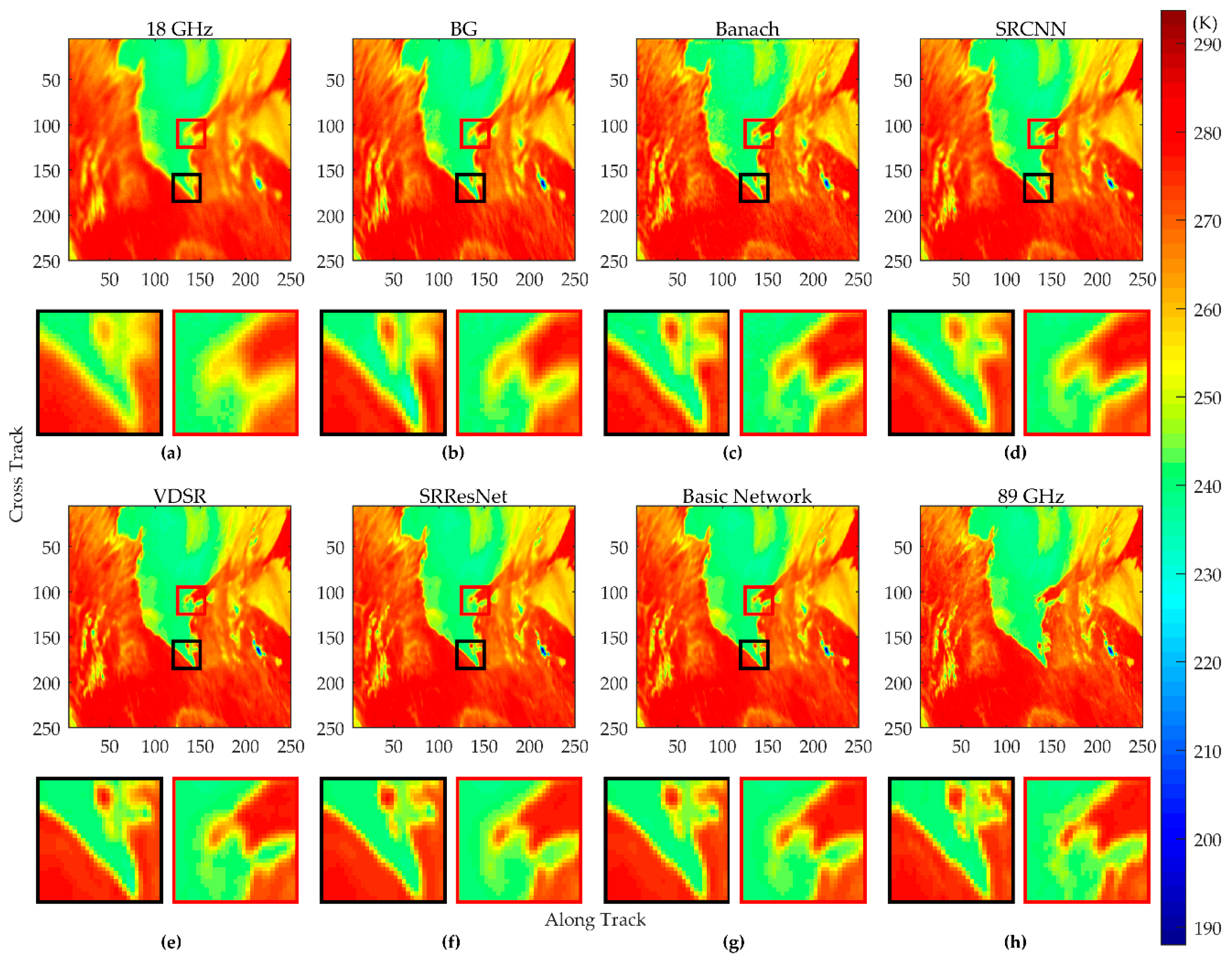
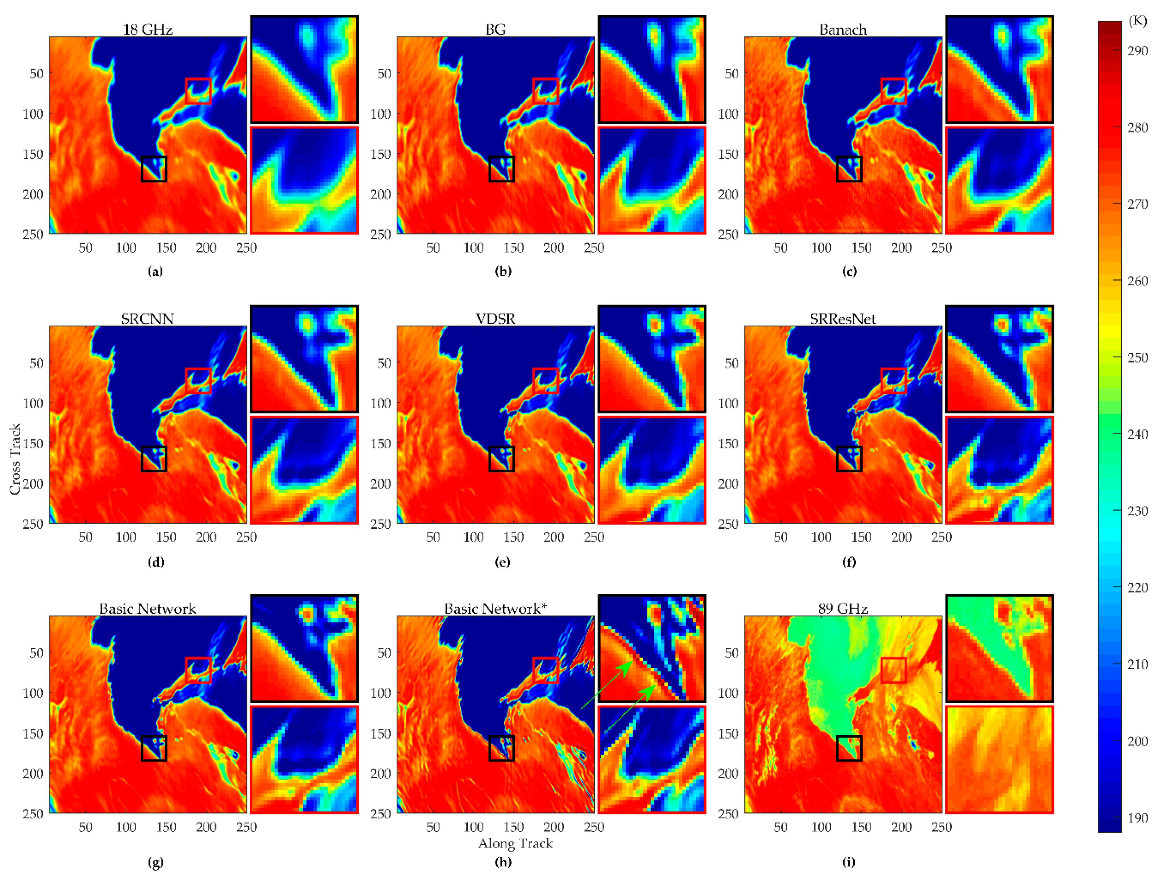
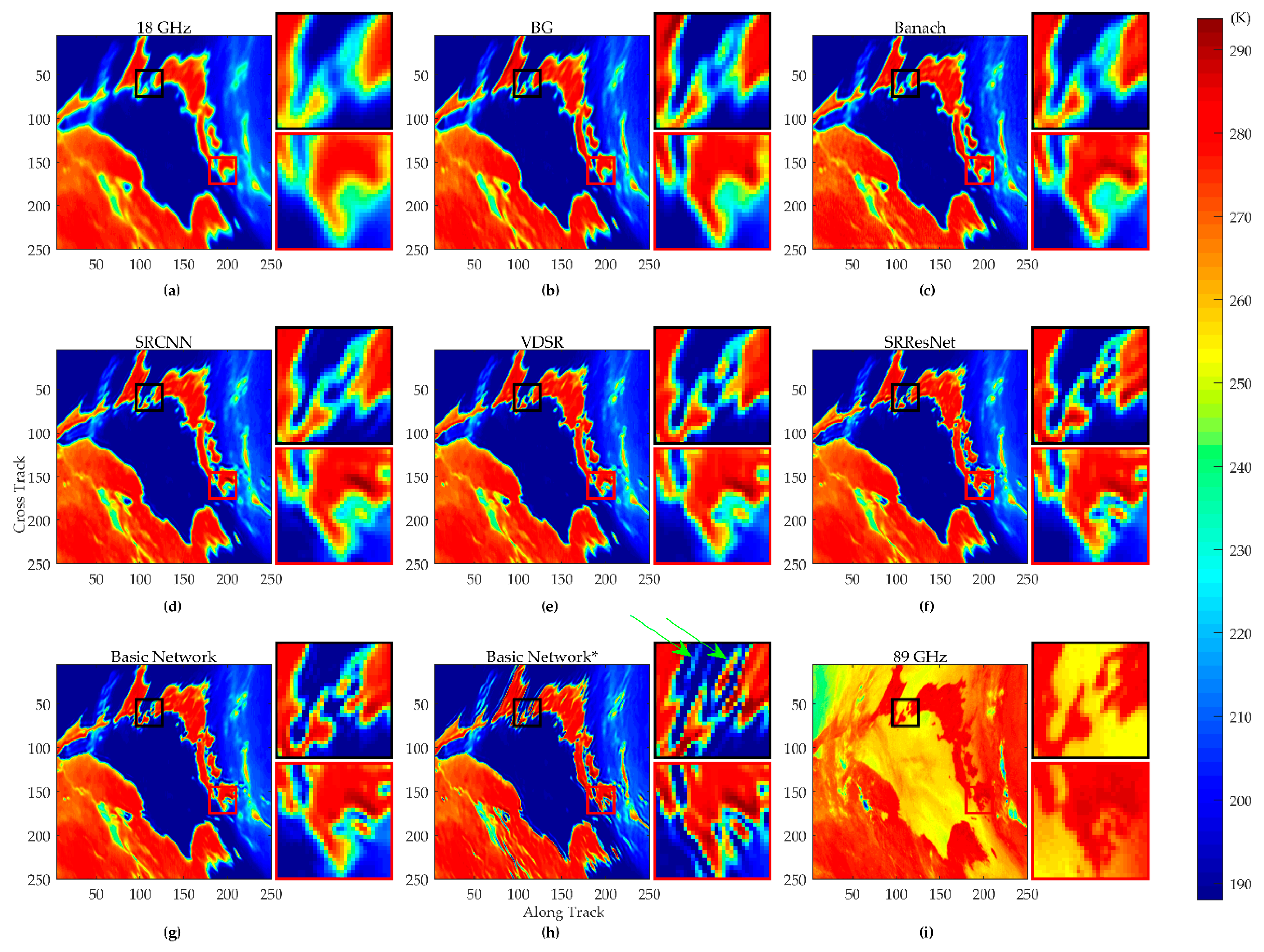
4.1.3. Real Data Testing

The above results show the superior resolution match ability of the deep residual CNN in the synthetic scenario and in the test set. However, the validity of the method to the MWRI real data is still sealed. Real 18.7 GHz data of FY-3C MWRI with horizontal polarization were used to demonstrate the effectiveness of our network in practical use. Since the 18.7 GHz ideal brightness temperature images are unavailable (no ideal label for real data testing), the real 89 GHz data of FY-3C MWRI with horizontal polarization are shown for reference in terms of spatial resolution. In addition, in order to evaluate the degradation model, the resolution match results of the same basic network based on the other model (Equations (10) and (11)) [17] are also shown for comparison.
Figure 11 shows the same area as Figure 10, and the enlarged areas show the Bol’shoy Shantar island (enclosed by the black rectangle, the same area as the Figure 10 black rectangle) and the southern part of Sakhalin island (enclosed by the red rectangle). Figure 11a shows the real 18.7 GHz data and Figure 11i shows the real 89 GHz data. Neglecting the different radiation characteristics of the two channels, the spatial resolution of Figure 11f, g was the closest to the 89 GHz channel through visual judgment. Although the southern part of Sakhalin island was shielded by cloud for the 89 GHz channel, as shown in the red rectangle in Figure 11i, due to the strong penetration ability of the low frequency channel, the emission from the earth surface could still be obtained through the 18.7 GHz observation. Among these methods, only the basic network and SRResNet had successfully recognized the lake below the Gulf of Patience, as shown in the red rectangle in Figure 11f, g. Furthermore, the resolution match result based on the degradation model (Equations (10) and (11)) [17] is shown in Figure 11h. All the other settings were kept the same as our method in order to implement a fair comparison. As can be seen, the match result is comparable with the 89 GHz data, but harmful artifacts were introduced, as shown with the green arrow in Figure 11h.
Figure 12 shows another test area around Japan; the top left and bottom right corner coordinates of the scenario were 53.6°N, 152.0°E and 30.3°N, 124.2°E, and the enlarged areas show the southern Hokkaido and the southern Kyushu islands. In this scene, our method also achieved an outstanding resolution match result with the 89 GHz channel, and severe artifacts were also introduced with the degradation model (Equations (10) and (11)), as shown with the green arrow in Figure 12h.
As for the model (Equations (10) and (11)), as we discussed in Section 3.1, the inaccurate estimation of the degradation model (blur kernel) that relates the LR/HR images may lead to sharpening artifacts (for this case) or over-smoothed results [27]. Furthermore, in this case, the noise amplification during the mapping process from Equations (10) to (11) (NEΔT of 89 GHz channel is 0.8 K, while the 18.7 GHz channel is 0.5 K) further deteriorated the results.
It is noted that the real 18.7 GHz antenna temperature images have different radiation characteristics and a little bit sharper gradient features than the LR images in the dataset, since the real data are degraded by the brightness temperature (although unavailable, illustrated in Equation (7)), while the LR images are degraded by the simulated brightness temperature (real 89 GHz data, shown in Equation (14)). Thus, the learning-based methods suffered from the adaptation problem to some extent. Even so, the basic network still achieved superior results. Because of the inaccessible label, the quantitative impact evaluation of this adaptation problem remained unattainable, which deserves further study.
All these evaluation results show that the fixed level resolution match ability of our basic network Nb is better than the advanced SRResNet by a small margin, and outperformed the other methods to a greater extent. In addition, the batch normalization (BN) layers in the SRResNet act in a similar way (the BN layer manipulates the statistics of the convolutional layer using the batch information while the AdaFM layer manipulates using the feature information) and are placed at the same position (right after the convolutional layer and ahead of the activation layer) with the AdaFM layers. Therefore, in order to implement the following network adaption for the other enhancement levels, we only chose a relatively simple structure CNN without the BN layers as our basic network. It should be mentioned here that other powerful and sophisticated CNNs can also be used to further explore the mapping ability and replace our basic network.

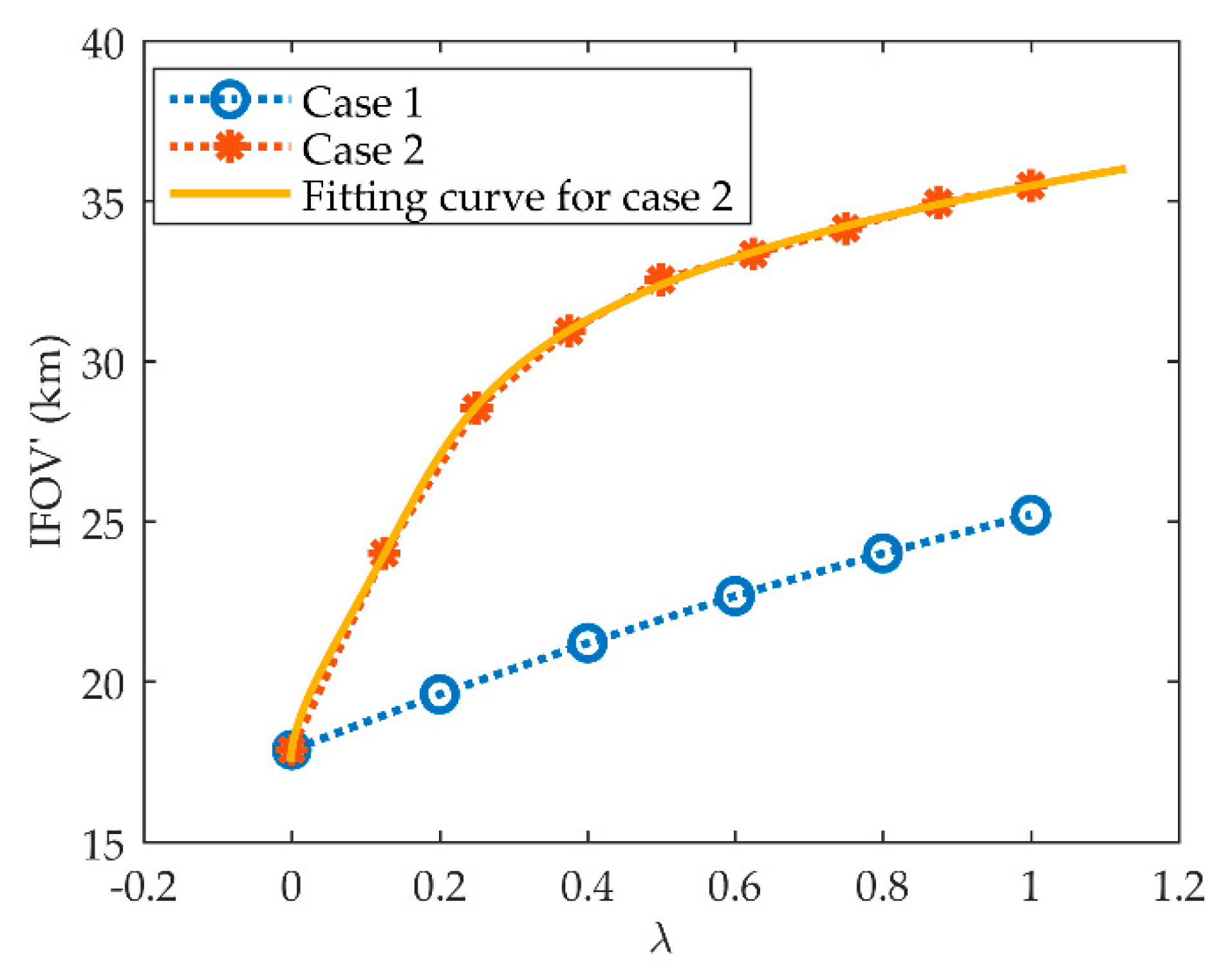
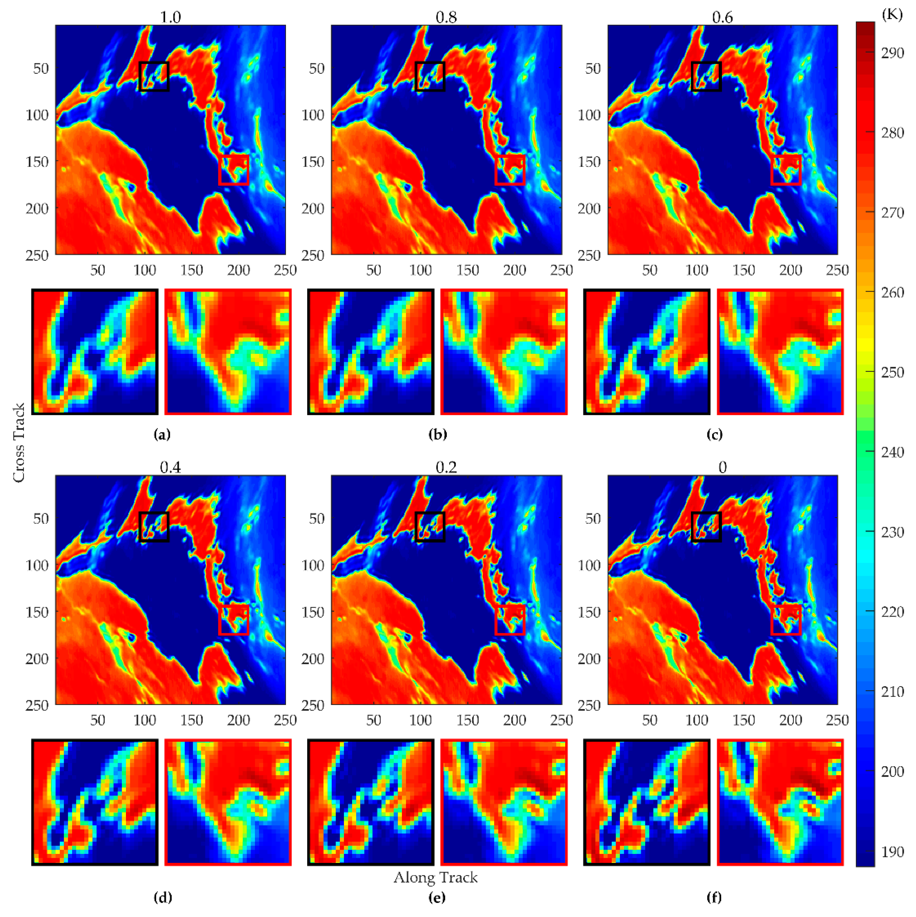
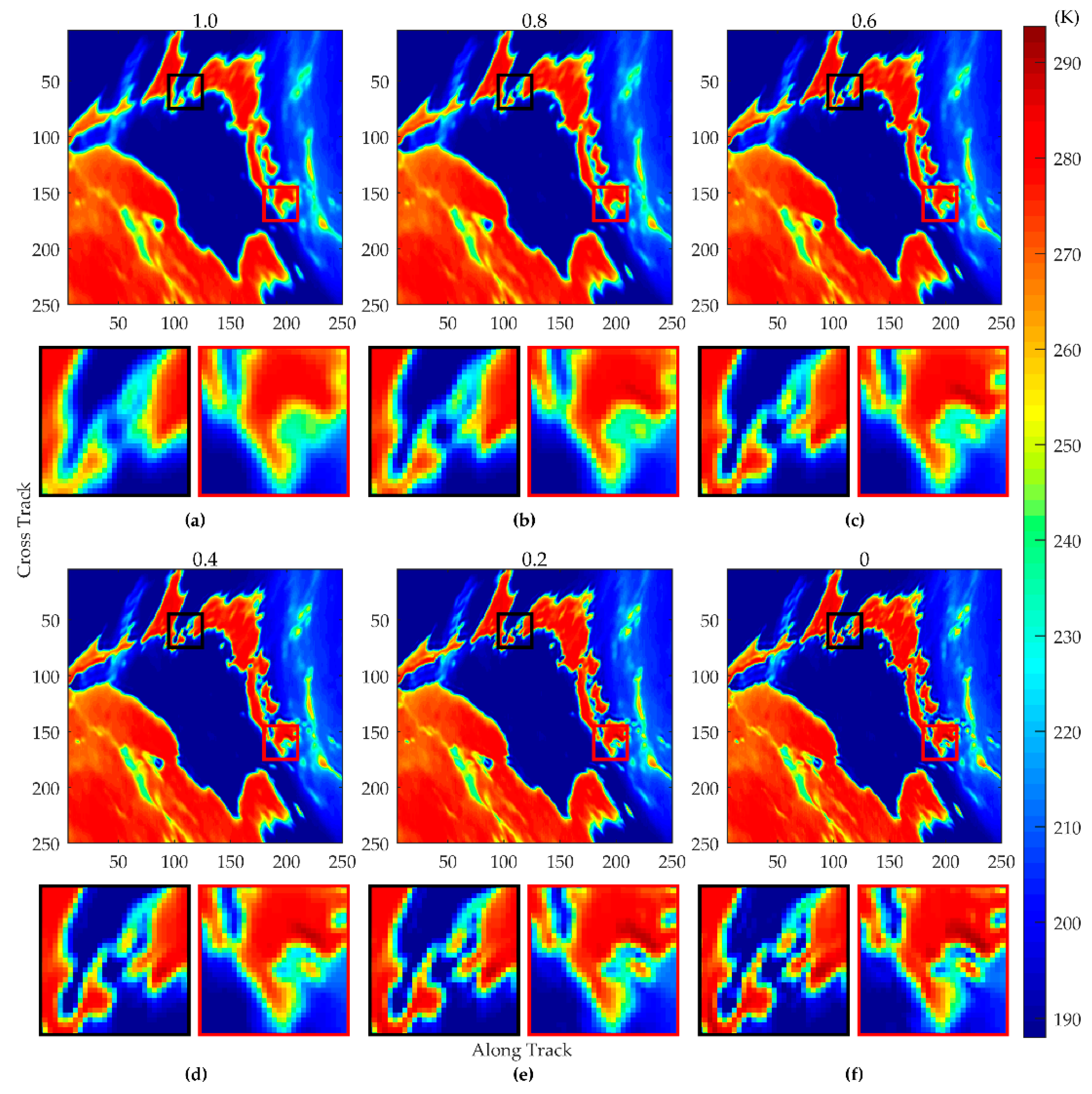
4.2. Resolution Match with Adjustable Network

4.2.1. Case 1 When vH1 = 89 GHz and vH2 = 36.5 GHz

As shown in the flowchart in Figure 6, based on dataset1 ( t L R s i m u m ( 18.7 ) and t H R 1 s i m u m ( 18.7 , 89 ) image pairs) and dataset2 ( t L R s i m u m ( 18.7 ) and t H R 2 s i m u m ( 18.7 , 36.5 ) image pairs), the basic network Nb and adaptive network Na could be trained. The test set evaluation gaps between the adaptive network Na (derived from the basic network Nb, and only optimized the additional 21,120 parameters in the AdaFM layers based on dataset2) and the network Na (trained all the 1,277,889 parameters in Na from scratch based on dataset2) were very small, as shown in Table 4. Thus, it proved the validity of our transfer training mode for the adaptive network Na when matching the resolution from 18.7 GHz to 36.5 GHz. Eventually, the adjustable network N a γ was created. By testing several typical output points in the test set, as shown with the blue line in Figure 13, we can see that the relationship between the IFOV’ (or γ) and λ was basically linear, thus we used T ( γ ) = γ in Equation (18) for this case.
In order to test the continuous and smooth resolution enhancement ability of the adjustable network N a γ , a few interpolation coefficients (γ = 0, 0.2, 0.4, 0.6, 0.8, and 1) were tested. The location information of the test scene was the same as Figure 12. When γ = 1, the network N a γ = 1 was equal to the adaptive network Na. Thus, the resolution was matched to the 36.5 GHz channel, as shown in Figure 14a. When γ = 0, the network N a γ = 0 was equal to the basic network Nb. At this time, the resolution was matched to the 89 GHz channel, as shown in Figure 14f. When the interpolation coefficient changed from 1 to 0, the result produced by the network N a γ smoothly and continuously changed from 36.5 GHz resolution to 89 GHz resolution, as shown in Figure 14. For instance, it is obviously exhibited in the red rectangular that the outline of the Amakusa main islands gradually becomes clearer as the interpolation coefficient decreases, which demonstrates the validity of the network. Note that we only need to train the basic network Nb and the adaptive network Na once, and no further training process is required for the adjustable network N a γ .

4.2.2. Case 2 When vH1 = 89 GHz and vH2 = 23.8 GHz

When v H 2 = 23.8   GHz , the evaluation gaps between the adaptive network Na and the network Na trained from scratch were still inconspicuous, as shown in Table 4. However, due to the larger resolution gap between the 23.8 GHz channel and the 89 GHz channel, the relationship between the IFOV’ (or γ) and λ was no longer linear, as shown with the red line in Figure 13. Thus, the fitted quartic polynomial function T ( γ ) = 2.84 γ 4 3.54 γ 3 + 1.57 γ 2 + 0.12 γ was used in Equation (18) to linearly map the interpolation coefficient γ to the spatial resolution.
The same scenario was also used for demonstration and comparison in this case, as shown in Figure 15. As can be seen, by tuning this controllable coefficient γ, the network could consecutively and smoothly manipulate the resolution enhancement level. Therefore, the effectiveness of the adjustable network in resolution match can be proved.

5. Discussion

Since the brightness temperature data is unavailable, in this paper, the datasets were made from the 89 GHz antenna temperature data due to their highest spatial resolution. In this way, we proposed a flexible degradation model to generate the datasets, so that a large amount of suitable learning pairs could be provided for training and testing of the network for various levels of matching problems. Using these datasets, our method produced better resolution match results than some of the state of the art methods. However, on the one hand, the 89 GHz channel is easily affected by atmospheric effects, which tends to smooth the antenna temperature images. Thus, methods to remove these atmospheric effects before making the LR/HR learning pairs need to be explored in future work. On the other hand, in order to address the adaptation problem, emulational brightness temperature scenarios could be used to generate the LR/HR dataset to further strengthen the method’s practical use.
For the degradation model, only four dominant factors, including the antenna pattern, the integration time, the scan geometry, and the receiver sensitivity, were considered. Other factors, for example the side lobes of the antenna pattern, could also be added to this model and then learned by the network. As for the network, we only used a simple but effective EDSR [29] alike network for our basic network Nb, but other sophisticated CNNs with a generative adversarial network (GAN) or auxiliary parallel branches could also be used to explore the better mapping results. Furthermore, the spatial resolution matched data could be used in the inversion of atmospheric parameters to further validate the effectiveness of our method.

6. Conclusions

An ASRM framework, based on the flexible degradation model, deep residual CNN, and adjustable AdaFM layers, is proposed to adaptively enhance and match the spatial resolution of satellite-based microwave radiometer data. Specifically, the degradation model is used to generate the adaptive datasets for various levels of matching tasks. Furthermore, for each fixed level, the deep residual CNN could produce better resolution matching results than some state of the art methods both quantitatively and qualitatively. In addition, with the help of AdaFM layers, the adjustable network could effectively handle arbitrary and continuous resolution matching problems between a start and an end level. Abundant experiments, executed both on the simulated and real scenarios, have demonstrated the superiority and validity of the method.

Author Contributions

Conceptualization, Y.L. and W.Z.; methodology, Y.L., S.C., W.Z., R.G., and J.H.; resources, W.H.; writing—original draft preparation, Y.L., S.C., and W.Z.; writing—review and editing, W.H., Y.L., and S.C.; supervision, L.L.

Funding

This research was funded by the National Natural Science Foundation of China, grant numbers 61527805, 61731001, and 41775030.

Acknowledgments

The authors would like to thank the National Satellite Meteorological Centre for providing the MWRI data of the FY-3C satellite.

Conflicts of Interest

The authors declare no conflict of interest.

References

  1. Ulaby, F.T.; Moore, R.K.; Fung, A.K. Microwave Remote Sensing: Active and Passive, Volume I: Microwave Remote Sensing Fundamentals and Radiometry; Artech House: Norwood, MA, USA, 1981. [Google Scholar]
  2. Yang, Z.; Lu, N.; Shi, J.; Zhang, P.; Dong, C.; Yang, J. Overview of FY-3 payload and ground application system. IEEE Trans. Geosci. Remote Sens. 2012, 50, 4846–4853. [Google Scholar] [CrossRef]
  3. Yang, H.; Weng, F.; Lv, L.; Lu, N.; Liu, G.; Bai, M.; Qian, Q.; He, J.; Xu, H. The FengYun-3 microwave radiation imager on-orbit verification. IEEE Trans. Geosci. Remote Sens. 2011, 49, 4552–4560. [Google Scholar] [CrossRef]
  4. Yang, H.; Zou, X.; Li, X.; You, R. Environmental data records from FengYun-3B microwave radiation imager. IEEE Trans. Geosci. Remote Sens. 2012, 50, 4986–4993. [Google Scholar] [CrossRef]
  5. Robinson, W.D.; Kummerow, C.; Olson, W.S. A technique for enhancing and matching the resolution of microwave measurements from the SSM/I instrument. IEEE Trans. Geosci. Remote Sens. 1992, 30, 419–429. [Google Scholar] [CrossRef]
  6. Wang, Y.; Shi, J.; Jiang, L.; Du, J.; Tian, B. The development of an algorithm to enhance and match the resolution of satellite measurements from AMSR-E. Sci. China Earth Sci. 2011, 54, 410–419. [Google Scholar] [CrossRef]
  7. Drusch, M.; Wood, E.F.; Lindau, R. The impact of the SSM/I antenna gain function on land surface parameter retrieval. Geophys. Res. Lett. 1999, 26, 3481–3484. [Google Scholar] [CrossRef]
  8. Tang, F.; Zou, X.; Yang, H.; Weng, F. Estimation and correction of geolocation errors in FengYun-3C Microwave Radiation Imager Data. IEEE Trans. Geosci. Remote Sens. 2016, 54, 407–420. [Google Scholar] [CrossRef]
  9. Sethmann, R.; Burns, B.A.; Heygster, G.C. Spatial resolution improvement of SSM/I data with image restoration techniques. IEEE Trans. Geosci. Remote Sens. 1994, 32, 1144–1151. [Google Scholar] [CrossRef]
  10. Long, D.G.; Daum, D.L. Spatial resolution enhancement of SSM/I data. IEEE Trans. Geosci. Remote Sens. 1998, 36, 407–417. [Google Scholar] [CrossRef] [Green Version]
  11. Hu, W.; Li, Y.; Zhang, W.; Chen, S.; Lv, X.; Ligthart, L. Spatial resolution enhancement of satellite microwave radiometer data with deep residual convolutional neural network. Remote Sens. 2019, 11, 771. [Google Scholar] [CrossRef]
  12. Stogryn, A. Estimates of brightness temperatures from scanning radiometer data. IEEE Trans. Antennas Propag. 1978, 26, 720–726. [Google Scholar] [CrossRef]
  13. Migliaccio, M.; Gambardella, A. Microwave radiometer spatial resolution enhancement. IEEE Trans. Geosci. Remote Sens. 2005, 43, 1159–1169. [Google Scholar] [CrossRef]
  14. Liu, D.; Liu, K.; Lv, C.; Miao, J. Resolution enhancement of passive microwave images from geostationary Earth orbit via a projective sphere coordinate system. J. Appl. Remote Sens. 2014, 8, 083656. [Google Scholar] [CrossRef] [Green Version]
  15. Lenti, F.; Nunziata, F.; Estatico, C.; Migliaccio, M. On the spatial resolution enhancement of microwave radiometer data in Banach spaces. IEEE Trans. Geosci. Remote Sens. 2014, 52, 1834–1842. [Google Scholar] [CrossRef]
  16. Hu, W.; Zhang, W.; Chen, S.; Lv, X.; An, D.; Ligthart, L. A deconvolution technology of microwave radiometer data using convolutional neural networks. Remote Sens. 2018, 10, 275. [Google Scholar] [CrossRef]
  17. Hu, T.; Zhang, F.; Li, W.; Hu, W.; Tao, R. Microwave Radiometer Data Superresolution Using Image Degradation and Residual Network. IEEE Trans. Geosci. Remote Sens. 2019, 1–14. [Google Scholar] [CrossRef]
  18. Dong, C.; Loy, C.C.; He, K.; Tang, X. Image super-resolution using deep convolutional networks. IEEE Trans. Pattern Anal. Mach. Intell. 2016, 38, 295–307. [Google Scholar] [CrossRef]
  19. Zhang, K.; Zuo, W.; Gu, S.; Zhang, L. Learning deep CNN denoiser prior for image restoration. In Proceedings of the IEEE Conference on Computer Vision and Pattern Recognition, Honolulu, HI, USA, 21–26 July 2017; pp. 2808–2817. [Google Scholar]
  20. Liu, X.; Jiang, L.; Wu, S.; Hao, S.; Wang, G.; Yang, J. Assessment of methods for passive microwave snow cover mapping using FY-3C/MWRI data in China. Remote Sens. 2018, 10, 524. [Google Scholar] [CrossRef]
  21. Yang, S.; Weng, F.; Yan, B.; Sun, N.; Goldberg, M. Special Sensor Microwave Imager (SSM/I) intersensor calibration using a simultaneous conical overpass technique. J. Appl. Meteorol. Climatol. 2011, 50, 77–95. [Google Scholar] [CrossRef]
  22. Wu, S.; Chen, J. Instrument performance and cross calibration of FY-3C MWRI. In Proceedings of the 2016 IEEE International Geoscience and Remote Sensing Symposium (IGARSS), Beijing, China, 10–15 July 2016; pp. 388–391. [Google Scholar]
  23. Piepmeier, J.R.; Long, D.G.; Njoku, E.G. Stokes antenna temperatures. IEEE Trans. Geosci. Remote Sens. 2008, 46, 516–527. [Google Scholar] [CrossRef]
  24. Di Paola, F.; Dietrich, S. Resolution enhancement for microwave-based atmospheric sounding from geostationary orbits. Radio Sci. 2008, 43, 1–14. [Google Scholar] [CrossRef]
  25. Gong, R.; Li, W.; Chen, Y.; Van Gool, L. DLOW: Domain flow for adaptation and generalization. In Proceedings of the IEEE Conference on Computer Vision and Pattern Recognition, Long Beach, CA, USA, 16–20 June 2019; pp. 2477–2486. [Google Scholar]
  26. He, J.; Dong, C.; Qiao, Y. Modulating image restoration with continual levels via adaptive feature modification layers. In Proceedings of the IEEE Conference on Computer Vision and Pattern Recognition, Long Beach, CA, USA, 16–20 June 2019; pp. 11056–11064. [Google Scholar]
  27. Efrat, N.; Glasner, D.; Apartsin, A.; Nadler, B.; Levin, A. Accurate blur models vs. image priors in single image super-resolution. In Proceedings of the IEEE International Conference on Computer Vision, Sydney, NSW, Australia, 1–8 December 2013; pp. 2832–2839. [Google Scholar]
  28. Kim, J.; Kwon Lee, J.; Mu Lee, K. Accurate image super-resolution using very deep convolutional networks. In Proceedings of the IEEE Conference on Computer Vision and Pattern Recognition, Las Vegas, NV, USA, 27–30 June 2016; pp. 1646–1654. [Google Scholar]
  29. Lim, B.; Son, S.; Kim, H.; Nah, S.; Lee, K.M. Enhanced deep residual networks for single image super-resolution. In Proceedings of the IEEE Conference on Computer Vision and Pattern Recognition (CVPR) Workshops, Honolulu, HI, USA, 21–26 July 2017; pp. 1132–1140. [Google Scholar]
  30. Szegedy, C.; Liu, W.; Jia, Y.; Sermanet, P.; Reed, S.; Anguelov, D.; Erhan, D.; Vanhoucke, V.; Rabinovich, A. Going deeper with convolutions. In Proceedings of the IEEE Conference on Computer Vision and Pattern Recognition, Boston, MA, USA, 7–12 June 2015; pp. 1–9. [Google Scholar]
  31. He, K.; Zhang, X.; Ren, S.; Sun, J. Deep residual learning for image recognition. In Proceedings of the IEEE Conference on Computer Vision and Pattern Recognition, Las Vegas, NV, USA, 27–30 June 2016; pp. 770–778. [Google Scholar]
  32. Damera-Venkata, N.; Kite, T.D.; Geisler, W.S.; Evans, B.L.; Bovik, A.C. Image quality assessment based on a degradation model. IEEE Trans. Image Process. 2000, 9, 636–650. [Google Scholar] [CrossRef] [PubMed]
  33. Zhao, H.; Gallo, O.; Frosio, I.; Kautz, J. Loss functions for image restoration with neural networks. IEEE Trans. Comput. Imaging 2017, 3, 47–57. [Google Scholar] [CrossRef]
  34. Wang, Z.; Bovik, A.C.; Sheikh, H.R.; Simoncelli, E.P. Image quality assessment: From error visibility to structural similarity. IEEE Trans. Image Process. 2004, 13, 600–612. [Google Scholar] [CrossRef]
  35. Ledig, C.; Theis, L.; Huszár, F.; Caballero, J.; Cunningham, A.; Acosta, A.; Aitken, A.P.; Tejani, A.; Totz, J.; Wang, Z. Photo-Realistic Single Image Super-Resolution Using a Generative Adversarial Network. In Proceedings of the IEEE Conference on Computer Vision and Pattern Recognition (CVPR), Honolulu, HI, USA, 21–26 July 2017; pp. 4681–4690. [Google Scholar]
Figure 1. Illustration of the accommodative spatial resolution match (ASRM) method.
Remotesensing 11 02432 g001
Figure 2. The scan geometry of the Fengyun-3C (FY-3C) microwave radiation imager (MWRI).
Remotesensing 11 02432 g002
Figure 3. The architecture of deep residual convolutional neural network (CNN).
Remotesensing 11 02432 g003
Figure 4. Schematic diagram of convolution operations. (a) Schematic diagram of convolution operation in the convolutional layer; (b) Schematic diagram of group convolution operation in the AdaFM layer.
Remotesensing 11 02432 g004
Figure 5. Illustration of resolution adjustment.
Remotesensing 11 02432 g005
Figure 6. The flowchart of the ASRM framework.
Remotesensing 11 02432 g006
Figure 7. The synthetic scenario and the resolution match results. (a) Simulated 18.7 GHz antenna temperature image; (b) Match result of the Backus–Gilbert (BG) method; (c) Match result of Banach method; (d) Match result of SRCNN; (e) Match result of VDSR; (f) Match result of SRResNet; (g) Match result of basic network Nb; (h) Simulated 89 GHz antenna temperature image; (i) Synthetic brightness temperature image.
Remotesensing 11 02432 g007
Figure 8. The along-track transects of the synthetic scenario. (a) The along-track transects around the strip (labeled with the blue dash-dotted line in Figure 7i); (b) The along-track transects around the background (labeled with the red dash-dotted line in Figure 7i).
Remotesensing 11 02432 g008
Figure 9. The evaluation indexes of the test set (3 points smoothed). (a) The PSNR results of the test set; (b) The SSIM results of the test set; (c) The IFOV’ results of the test set.
Remotesensing 11 02432 g009
Figure 10. A pair of test set images and their resolution match results. (a) Simulated 18.7 GHz antenna temperature image; (b) Match result of the BG method; (c) Match result of the Banach method; (d) Match result of SRCNN; (e) Match result of VDSR; (f) Match result of SRResNet; (g) Match result of basic network Nb; (h) Simulated 89 GHz antenna temperature image.
Remotesensing 11 02432 g010
Figure 11. Resolution match results of real 18.7 GHz MWRI data. (a) Real 18.7 GHz antenna temperature image; (b) Match result of the BG method; (c) Match result of the Banach method; (d) Match result of SRCNN; (e) Match result of VDSR; (f) Match result of SRResNet; (g) Match result of basic network Nb; (h) Match result of basic network Nb with degradation model (Equations (10) and (11)); (i) Real 89 GHz antenna temperature image.
Remotesensing 11 02432 g011
Figure 12. Resolution match results of real 18.7 GHz MWRI data. (a) Real 18.7 GHz antenna temperature image; (b) Match result of the BG method; (c) Match result of the Banach method; (d) Match result of SRCNN; (e) Match result of VDSR; (f) Match result of SRResNet; (g) Match result of basic network Nb; (h) Match result of basic network Nb with degradation model (Equations (10) and (11)); (i) Real 89 GHz antenna temperature image.
Remotesensing 11 02432 g012
Figure 13. Typical output points of the adjustable network N a γ and its fitting curve.
Remotesensing 11 02432 g013
Figure 14. Resolution enhancement results by adjustable network N a γ . (a) Output of adjustable network N a γ when γ = 1 (the resolution is matched to the 36.5 GHz channel); (b) Output when γ = 0.8; (c) Output when γ = 0.6; (d) Output when γ = 0.4; (e) Output when γ = 0.2; (f) Output when γ = 0 (the resolution is matched to the 89 GHz channel).
Remotesensing 11 02432 g014
Figure 15. Resolution enhancement results by adjustable network N a γ . (a) Output of adjustable network N a γ when γ = 1 (the resolution is matched to the 23.8 GHz channel); (b) Output when γ = 0.8; (c) Output when γ = 0.6; (d) Output when γ = 0.4; (e) Output when γ = 0.2; (f) Output when γ = 0 (the resolution is matched to the 89 GHz channel).
Remotesensing 11 02432 g015
Table 1. Performance of the FY-3C MWRI.
Frequency (GHz)PolarizationIFOV (km)Sensitivity NEΔT (K)Integration Time (ms)
10.65V/H51 × 850.515.0
18.7V/H30 × 500.510.0
23.8V/H27 × 450.57.5
36.5V/H18 × 300.55.0
89.0V/H9 × 150.82.5
Table 2. The averaged evaluation indexes of the synthetic scenario.
MethodsPSNR (dB)SSIMIFOV’ (km)Noise
18 GHz37.6010.94540.000.501
BG38.9620.96026.850.535
Banach40.7760.96623.730.700
3-layer CNN39.6120.96228.250.401
VDSR42.5010.98021.630.284
SRResNet43.0770.98321.350.140
Basic Network43.1340.98320.760.200
Table 3. The evaluation indexes of the test set.
Test ScenesIndexes18 GHzBGBanachSRCNNVDSRSRRestNetBasic Network
Scene 33PSNR (dB)44.45946.40047.61947.88849.61950.43350.617
SSIM0.9800.9860.9870.9890.9920.9930.993
IFOV’ (km)39.7325.7321.7324.9319.3318.1318.13
Scene 48PSNR (dB)47.10447.88349.15149.23850.18548.07050.716
SSIM0.9830.9870.9880.9890.9910.9910.992
IFOV’ (km)40.1326.1323.5327.3324.1322.9322.93
Scene 78PSNR (dB)48.55049.74850.24851.98653.88454.54454.544
SSIM0.9910.9930.9920.9950.9960.9970.997
IFOV’ (km)39.7326.1320.9323.7319.3318.9318.13
Scene 104PSNR (dB)41.45943.01844.95344.62446.14146.88247.037
SSIM0.9600.9730.9780.9780.9830.9860.986
IFOV’ (km)40.1326.1322.5324.5320.9319.3319.33
Scene 193PSNR (dB)41.12942.68443.78244.52346.50147.01047.390
SSIM0.9640.9740.9780.9810.9860.9880.989
IFOV’ (km)39.7327.7324.9324.5319.7317.7317.73
200 Scenes AveragePSNR (dB)45.64646.69247.98348.58850.13250.53850.816
SSIM0.9820.9870.9880.9900.9920.9930.993
IFOV’ (km)39.9425.9422.7025.2020.9920.1219.82
Table 4. The evaluation results for adaptive network Na with different training methods.
CaseNetworkPSNR (dB)SSIMIFOV’ (km)
1: vH2 = 36.5 GHzNa (trained from Nb)57.780.998626.16
Na (trained from scratch)57.830.998626.23
2: vH2 = 23.8 GHzNa (trained from Nb)65.660.999735.83
Na (trained from scratch)65.480.999835.76

