A hybrid OSVM-OCNN Method for Crop Classification from Fine Spatial Resolution Remotely Sensed Imagery

Abstract

Accurate information on crop distribution is of great importance for a range of applications including crop yield estimation, greenhouse gas emission measurement and management policy formulation. Fine spatial resolution (FSR) remotely sensed imagery provides new opportunities for crop mapping at a detailed level. However, crop classification from FSR imagery is known to be challenging due to the great intra-class variability and low inter-class disparity in the data. In this research, a novel hybrid method (OSVM-OCNN) was proposed for crop classification from FSR imagery, which combines a shallow-structured object-based support vector machine (OSVM) with a deep-structured object-based convolutional neural network (OCNN). Unlike pixel-wise classification methods, the OSVM-OCNN method operates on objects as the basic units of analysis and, thus, classifies remotely sensed images at the object level. The proposed OSVM-OCNN harvests the complementary characteristics of the two sub-models, the OSVM with effective extraction of low-level within-object features and the OCNN with capture and utilization of high-level between-object information. By using a rule-based fusion strategy based primarily on the OCNN’s prediction probability, the two sub-models were fused in a concise and effective manner. We investigated the effectiveness of the proposed method over two test sites (i.e., S1 and S2) that have distinctive and heterogeneous patterns of different crops in the Sacramento Valley, California, using FSR Synthetic Aperture Radar (SAR) and FSR multispectral data, respectively. Experimental results illustrated that the new proposed OSVM-OCNN approach increased markedly the classification accuracy for most of crop types in S1 and all crop types in S2, and it consistently achieved the most accurate accuracy in comparison with its two object-based sub-models (OSVM and OCNN) as well as the pixel-wise SVM (PSVM) and CNN (PCNN) methods. Our findings, thus, suggest that the proposed method is as an effective and efficient approach to solve the challenging problem of crop classification using FSR imagery (including from different remotely sensed platforms). More importantly, the OSVM-OCNN method is readily generalisable to other landscape classes and, thus, should provide a general solution to solve the complex FSR image classification problem.

1. Introduction

Accurate crop distribution information from regional-to-global scales is essential for estimating crop yield [1], modelling greenhouse gas (GHG) emissions from agriculture [2] and making effective agrarian management policies [3]. Moreover, agricultural ecosystems are often managed intensively and modified frequently [4], which might alter land cover/use patterns rapidly and, thus, influence ecological processes and biogeochemical cycles [5]. These spatial and temporal characteristics pose a great challenge for traditional approaches (e.g., ground surveys) to monitoring agricultural systems. Remote sensing using sensors onboard satellite and aircraft platforms, however, has been shown to be an effective means of crop monitoring at regional-to-global scales, and has the advantages of being consistent, timely and cost-efficient (e.g., [2,5]).

Coarse and medium spatial resolution multispectral data, such as Landsat, SPOT and MODIS (Moderate Resolution Imaging Spectroradiometer), have been used widely for crop classification and mapping [3,6,7]. However, the accuracy of crop maps generated from these images is inevitably compromised by the spatial limitation [8], especially over the highly fragmented and heterogeneous agricultural areas. As stated by [9], a spatial resolution of less than 10 m is required for precision agriculture. More recently, remotely sensed imagery from fine spatial resolution (FSR) (<10 m) satellite systems (e.g., RapidEye, IKONOS, and WorldView) as well as airborne systems (e.g., Uninhabited Aerial Vehicle Synthetic Aperture Radar (UAVSAR)) is now available commercially, providing new opportunities for crop classification and mapping in very fine detail [9,10]. However, high intra-class variance and low inter-class separability over croplands in FSR images may exist because of differences in climatic conditions, topographic properties, soil composition, farming practices and so on [11]. Moreover, FSR imagery has fewer multispectral bands (around four) in comparison to medium resolution data (e.g., MODIS and Landsat), which leads to subtle differences in spectral/polarimetric properties amongst crop types (i.e., crop types are difficult to discriminate). Therefore, developing advanced classification methods for accurate crop mapping and monitoring is of prime concern, especially with a view to exploiting the deep hierarchical features presented in FSR imagery.

During the past few decades, a vast array of methods has been developed for remote sensing image classification [12,13,14]. These methods can be categorised into pixel-based and object-based methods according to the basic unit of analysis (either per-pixel or per-object) [15]. Pixel-based classification methods that rely purely upon spectral (or polarimetric) signatures have been used widely for crop classification using various types of imagery (including the newly-launched Sentinel-2 imagery [16,17,18]). However, these methods often produce limited classification accuracy due to large intra-class variances as stated above. Severe salt-and-pepper effects may occur owing to the noise in FSR imagery. Although some post-classification algorithms (e.g., spatial filters) might alleviate the noise to some extent, they may also erase small objects of interest comprised of just a few pixels. Compared with pixel-wise algorithms, object-based image analysis (OBIA) built upon segmented homogeneous objects [15] is preferable for crop classification using FSR remotely sensed images (e.g., [19,20], in which objects instead of pixels are adopted as the basic unit of analysis. This allows spatial information (e.g., texture, shape) with respect to the objects to be incorporated into the classification process, thus, reducing the salt-and-pepper noise [15].

Under the framework of OBIA, machine learning algorithms (e.g., the support vector machine (SVM), the multilayer perceptron (MLP) and the random forest (RF)) have been used for crop classification and mapping thanks to their ability to deal with multi-modal and noisy data [21]. The SVM, as a typical non-parametric machine learning classifier, was often found to outperform other machine learning algorithms in image classification due to its high generalisation ability [22]. The objected-based SVM (OSVM) has, thus, been popular for complex crop classification tasks [2,23]. In the OBIA classification process, there are generally two kinds of information that can be obtained from a spatially segmented region: within-object information (such as spectra, polarization, texture) and between-object information (such as configuration and topological relationships between adjacent objects) [24]. The OSVM classifier can extract within-object features (low-level information) from FSR images for classification. However, it is essentially a single-layer classifier (linear SVM) or two-layer classifier (kernel SVM) [25], which might overlook the high-level between-object information that may be critical to crop identification. For example, crop swath direction conveys important information for the identification of crop pattern [26]. In this context, a series of object-based spatial contextual descriptive indicators were developed based on spatial metrics, graphs and ontologies [27,28] to derive high-level semantic information from FSR images. However, it is often very difficult to characterise the spatial contexts as a set of “rules” in view of the structurally complicated and diverse agricultural landscapes [2], even if these complex spatial patterns might be interpreted by human experts [29].

Recent developments in artificial intelligence and pattern recognition demonstrated that high-level feature representations can be extracted with multi-layer neural networks in an “end-to-end” manner without using human-crafted “rules” [30]. These breakthrough deep learning algorithms achieved unprecedented success in a wide range of challenging domains, such as speech recognition, visual object recognition and target detection [30,31]. As a representative deep learning method, convolutional neural networks (CNNs) have drawn a lot of academic and industrial interest, and made huge improvements in the field of image analysis, such as text recognition [32], speech detection [31] and image denoising [33]. CNNs, with great capability in high-level feature characterization, were also applied to various remote sensing applications, such as object detection [34], image segmentation [35] and scene classification [36]. In addition, CNN-based approaches have been developed to solve the complex problem of remote sensing classification, where all pixels in an image are labelled into several categories. For example, Stoian, et al. [37] presented a fully-realized CNN model for land cover classification using multi-temporal high spatial resolution imagery. Chen, et al. [25] proposed a three-dimensional (3D) CNN for hyperspectral image classification by using both spectral and spatial features. Recently, Zhang, et al. [38] provided a novel approach by combining CNNs with rough sets for classification of FSR images. The above-mentioned work has achieved promising classification results, demonstrating the advantages of CNNs with respect to spatial feature representation. However, these pixel-based CNNs classify images by applying contextual patches as inputs, which often blurs the boundaries between adjacent ground objects, leading to over-smooth classification results [38]. To overcome this problem, a new object-based CNN (OCNN) framework was presented which combined the OBIA and CNN techniques, such that the segmented objects can be identified while retaining precise boundary information [24]. The OCNN method was applied to the complex land use classification task and produced encouraging classification results. However, with a fix-sized input window (receptive field), large uncertainties may be introduced into the OCNN classification process, especially for those objects with areas far smaller or larger than the input window [24]. Moreover, while the CNN model can explore the high-level features hidden in remotely sensed images, low-level features (e.g., within-object spectra) observed by shallow models may be overlooked [38].

Any single classifier is unlikely to achieve promising results if the scenes of remotely sensed imagery are complex [38,39]. The combination of multiple classification methods with complementary behaviours would be a good idea to improve complex land cover classification [40] and crop classification [39], by better exploring the minute differences that may exist between the classes. Within the remote sensing community, there are generally three types of ensemble-based systems, namely “consensus classification’’, ‘‘multiple classifier systems’’ and ‘‘decision fusion’’ [41]. Relying on multiple types of datasets, the utility of consensus classification is constrained due to the lack of availability of such data. By means of manipulating training samples to generate subsets randomly (boosting and bagging) [42], multiple classifier systems require extremely large sample sizes and deliver high time complexity. In contrast, decision fusion that combines the outputs of individual classifiers with a certain fusion rule to take advantage of complementary characteristics is a generally effective ensemble strategy [40]. For example, different classifiers may produce accurate results over different areas within a classification map and, hence, produce complementary results [38]. However, the above-mentioned ensemble methods are always performed based on pixel-wise classifiers with shallow structures and, thus, are not well suited to cope with the complex FSR image classification problem.

In this research, a novel OSVM-OCNN approach was proposed by combining the OSVM (an object-based SVM model with shallow architectures) and the OCNN (an object-based CNN model with deep architectures) through a rule-based decision fusion strategy. Image segmentation was first used to partition the agricultural landscape into basic crop patches (objects), based on whether the SVM and CNN models were respectively applied to allocate a label to each object. The outputs of the two models were combined subsequently through a rule-based fusion strategy according to prediction probability output from the CNN. Such a fusion decision strategy allows the rectification of CNN predictions with low confidence using SVM predictions at the object level. The major contributions of this research can be summarised as: (1) the shallow architecture SVM and the deep architecture CNN was first found to be complementary to each other in terms of crop classification at the object level; (2) a straightforward rule-based decision fusion strategy was developed to effectively fuse the results of the OSVM and OCNN. We investigated the effectiveness of the proposed approach over two study sites with heterogeneous agriculture landscapes in California, USA, using the FSR UAVSAR and RapidEye imagery.

The reminder of this paper is organised into five sections: Section 2 elaborates the proposed methods in detail. Section 3 provides the study area, datasets, model structure and experimental results. A thorough discussion of the observed results is made in Section 4, and the conclusions of this research are drawn in Section 5.

2. Method

2.1. Overview of the Support Vector Machine (SVM)

The principle of the SVM is to determine an optimal classification hyperplane by which a maximum margin can be achieved to separate the dataset into a predefined number of classes [43]. In this case, a kernel function, with additional variables, is usually adopted to map the non-linear input vectors into a higher space (e.g., Euclidean) $\Phi \left(X\right)$.

Suppose there is a set of data $(x_1,y_1),(x_2,y_2),\dots ,(x_m,y_m)$ distributed in the multi-dimensional feature space $X$, where $x_i$ denotes a sample vector with $y_i\in \left\{-1,+1\right\}$ as the corresponding target. The hyperplane in the transformed space can be defined as follows:

$$f\left(x\right)=\omega ·\Phi \left(x\right)+b$$

(1)

where $\omega$ denotes the weight vector of the hyperplane, and $b$ represents the offset of the hyperplane. The SVM cost function is defined using the following equations:

$${\min }_{\omega ,b,\epsilon }J\left(\omega ,b,\epsilon \right)=\frac{1}{2}{\left|\right|\omega \left|\right|}^2+C{\displaystyle {\displaystyle \sum }_{i=1}^m}{\epsilon }_i$$

(2)

subject to:

$$y_i\left(\omega \left(x_i^{\mathrm{T}}·x_j\right)+b\right)\ge 1-{\epsilon }_i,i=1,\dots ,m.$$

(3)

where ${\epsilon }_i$ denotes the slack variables, and $C$ refers to the penalty parameter used to control the trade-off between empirical risk and model complexity.

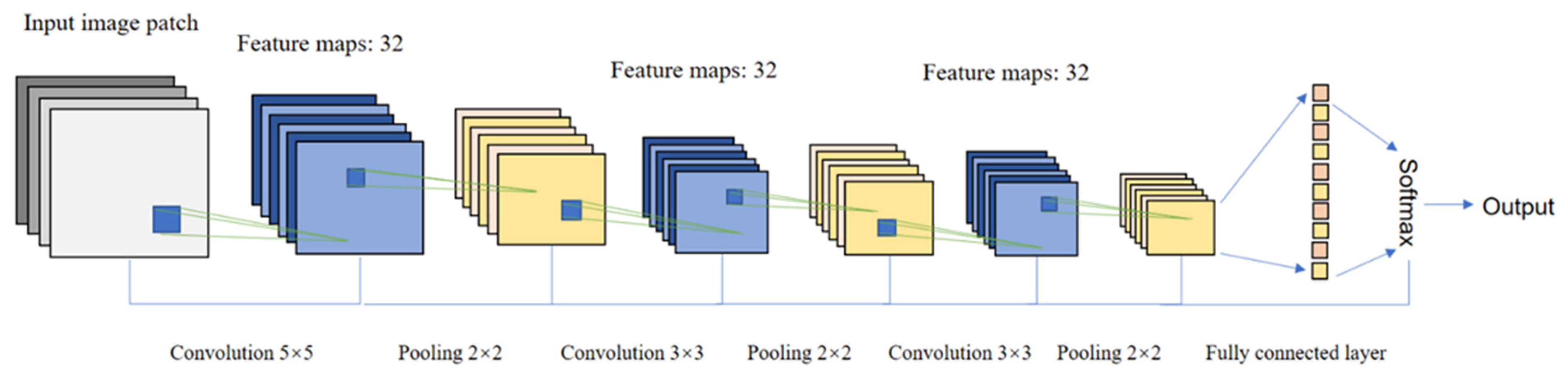
2.2. Overview of Convolutional Neural Networks (CNNs)

The CNN is a forward neural network that includes an input layer, multi-hidden layers and output layer, which are connected to each other with the output of the previous layer being the input of the next layer. High-level features contained in the raw data are extracted gradually through implementation of both a convolutional layer and a pooling/subsampling layer. To learn nonlinear representations of input data, a nonlinear activation function (e.g., sigmoid, rectified linear units) is adopted [31]. In general, the operations performed in a CNN can be summarised as:

$${\mathrm{O}}^l={\mathrm{pool}}_p\left(\sigma \left({\mathrm{O}}^{l-1}\ast w^l+b^l\right)\right)$$

(4)

where ${\mathrm{O}}^{l-1}$ represents the input to the $l$th layer, $w^l$ and $b^l$ are the weights and biases of the layer, respectively, $\sigma (·)$ indicates the non-linearity function and the symbol $\ast$ denotes linear convolution; a pooling operation (${\mathrm{pool}}_p$) with a window size $p$ is often performed following the convolution operation to extract invariant features of the input map, forming the output (${\mathrm{O}}^l$) of the current ($l$th) layer.

The feature maps outputted by the last pooling layer are then flattened into a one-dimensional array and classified using a logistic regression (LR). A softmax activation function is employed in the LR to ensure the prediction probability of each output unit belonging to a certain class sums to one.

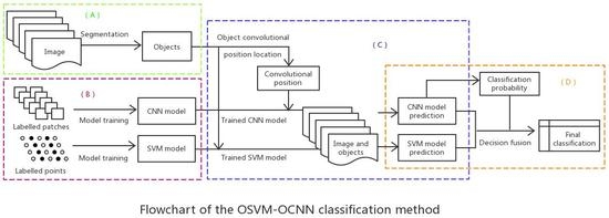
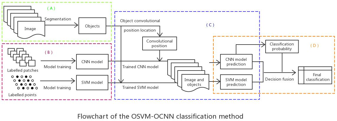
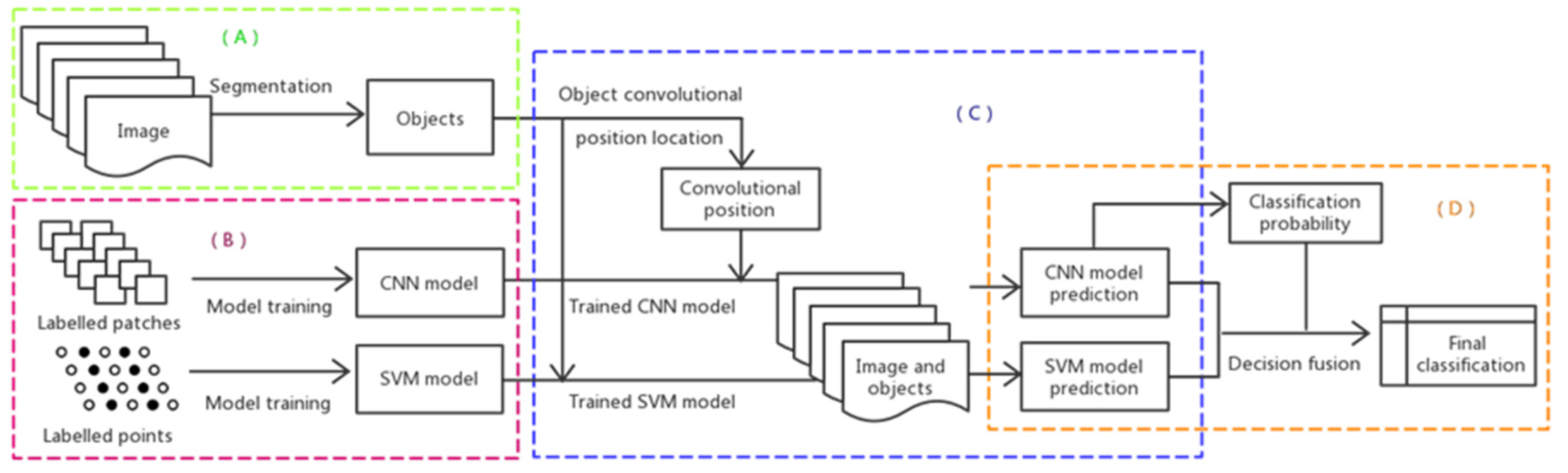
2.3. Hybrid Object-based SVM and CNN (OSVM-OCNN) Approach

We propose a novel hybrid object-based SVM and CNN (OSVM-OCNN) approach for crop classification from FSR remotely sensed imagery. In brief, the trained SVM and CNN models were used to predict the class of each segmented object, respectively, and a fusion strategy was applied subsequently to combine the two classifications to achieve the final classification map. Figure 1 shows the workflow of the presented OSVM-OCNN methodology, which comprises four steps, namely (1) image segmentation, (2) SVM and CNN model training, (3) SVM and CNN model inference and (4) decision fusion of SVM and CNN predictions, details of which will be elaborated in the following sections.

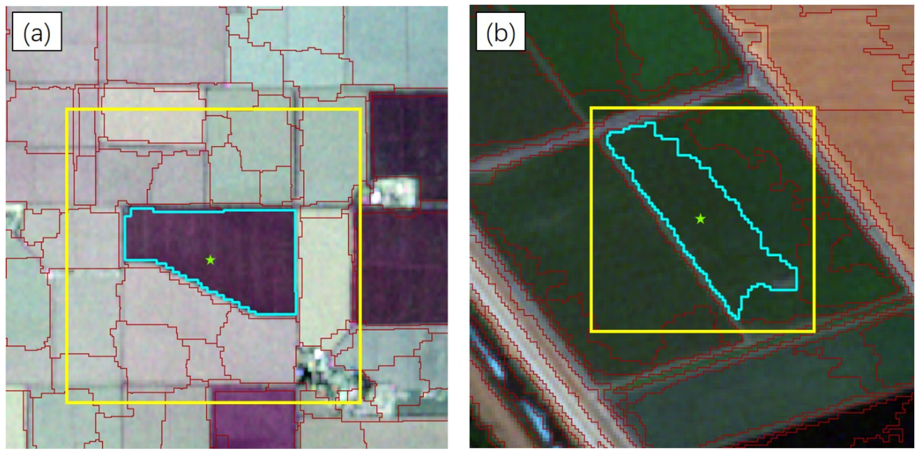
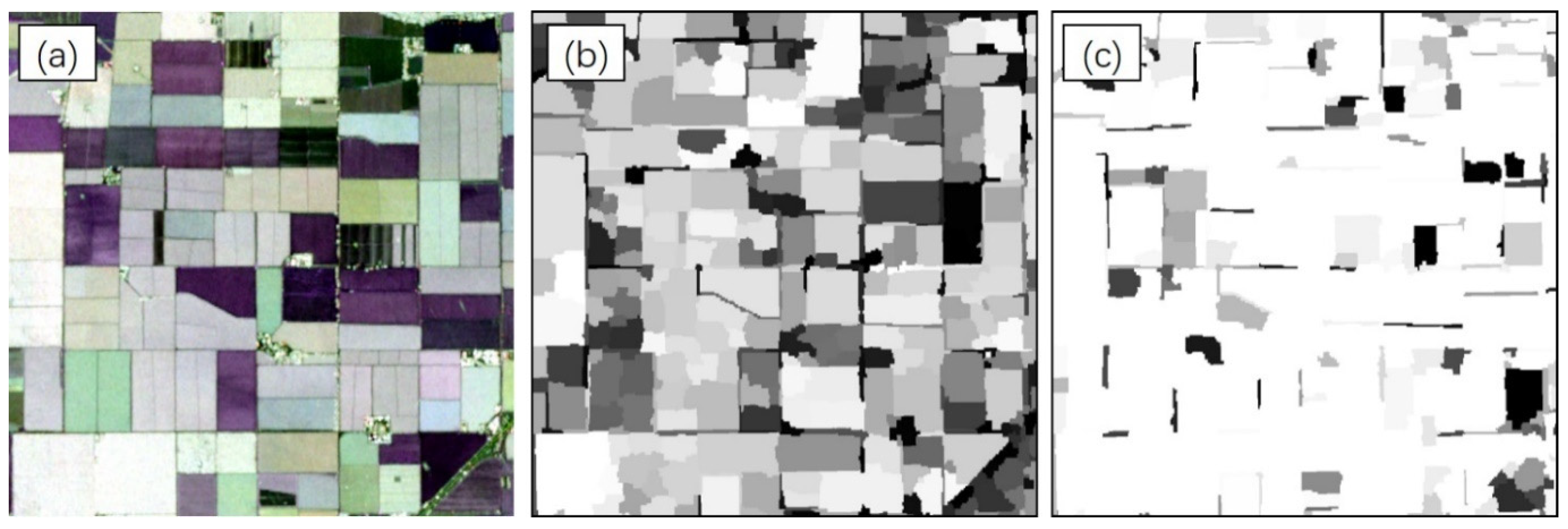
2.3.1. Image Segmentation

Image segmentation is considered the fundamental step of the OSVM-OCNN as the prediction procedures of both SVM and CNN modules are based on segmented image objects (Figure 1). In this research, the widely used multi-resolution segmentation (MRS) algorithm was adopted to partition the imagery into crop patches (i.e., objects) with spectrally and spatially homogeneous information [44]. For the fully polarimetric UAVSAR data, three raw linear polarizations (bands HH, HV, VV) together with polarimetric parameters from the Cloude-Pottier (entropy, anisotropy, and alpha angle) and Freeman-Durden (fractions of double-bounce, single-bounce, and volume scatters) decompositions [45,46] were combined as input data for image segmentation. As for the optical RapidEye imagery, all five multispectral (Blue, Green, Red, Red Edge and Near Infrared) bands were used as input for segmentation.

2.3.2. SVM and CNN Model Training

In this research, the radial basis function (RBF) SVM was selected owing to its capacity to address complicated non-linear classification problems [47]. The SVM model was trained using the spectral (or polarimetric) information within the segmented patches. Two types of feature were extracted from each object for classification, including the mean and standard deviation of feature bands. All these object-based hand-crafted features were fed into the SVM model for classification. Different from the SVM model, the image patches used to train the CNN model were extracted using a pre-defined square input window rather than segmented patches. The input window size and a range of parameters of the CNN model were tuned empirically, as detailed in Section 3.

The trained SVM and CNN models were used for the following model interference.

2.3.3. SVM and CNN Model Inference

At the model inference stage, the trained SVM was used directly to predict the label of each segmented object based on the hand-crafted features mentioned above. The inference procedure of the CNN model consists of two steps: the convolutional position of an object was first located to acquire the input image patch of CNN; then, the label of the object was predicted with the trained CNN model with the located convolutional positions and input image patches. To acquire representative features of crop patches, the object convolutional position should be located at the centre of each object. In this research, the convolutional position of each object was determined by its geometric centroid [48]. Figure 2 provides two examples of object convolutional position location.

For a specific object, its crop class is inferred by the trained CNN model; at the same time, the SVM model also allocates a class label to the object. Thus, each object has two predictions coming from the SVM and CNN models.

2.3.4. Decision Fusion of the SVM and CNN Models

For each object, the predictions of the SVM and CNN models are $m$-dimensional vectors $P=\left(p_1,p_2,\dots ,p_m\right)$, where $m$ is the number of classes, and each dimension $i\in \left[1,2,\dots ,m\right]$ denotes the predictive probability of the $i\mathrm{th}$ class. Ideally, the prediction probability should be 1 for the target class and 0 for the others. However, this is not likely to happen in consideration of the complexity of remotely sensed data. The probability for each class can be represented as $f\left(x\right)=\left\{p_x\right|x\in \left[1,2,\dots ,m\right]\}$, where $p_x\in \left[0,1\right]$ and ${{\displaystyle \sum }}_1^m{p}_x=1$. The SVM and CNN models simply classify each object into the class with the maximum membership ($\mathrm{class}\left(C\right)$) across all classes as follows:

$$\mathrm{class}\left(C\right)=\mathrm{argmax}\left(\left\{f\left(x\right)=p_x|x\in \left[1,2,\dots ,m\right]\right\}\right)$$

(5)

For a specific segmented object, the SVM model uses only the features that fall completely within the object (within-object information) for classification. As a result, objects with distinctive low-level features (e.g., light regions in Figure 3b) can be separated easily by the SVM, regardless of the size of objects. However, SVMs cannot identify accurately those objects with similar within-object features (e.g., dark regions in Figure 3b), due to the lack of contextual information in the classification process. In contrast, the CNN model can extract deep high-level features (between-object information) for classification and, thus, is superior to the SVM in identifying complex objects. Note that the CNN uses a pre-defined square input window to extract features and predict labels of objects. As a result, for a specific patch, there are two situations to consider: (1) if the size of the target object (e.g., small-sized) mismatches with the scale of input window (i.e., a large area of other crop types as contextual information in the input window), the prediction probability of the object tends to be low (e.g., dark patches in Figure 3c); (2) if the input window covers only a homogeneous region, the probability tends to be large (e.g., light patches in Figure 3c).

In light of the above-mentioned complementarities of the SVM and CNN, a rule-based fusion strategy can be presented to combine the two models for increased classification accuracy. The fusion output gives credit to the CNN if its prediction probability is greater than or equal to a predefined threshold ($\alpha$); otherwise, it trusts the output of the SVM. Assume an image is segmented into $N$ objects. For a given segmented object ($O_i$), where $i=1,2,\dots ,N$, a decision fusion strategy can be formulated to determine the class label ($class\left(O_i\right)$) of the object as follows:

$$class\left(O_i\right)=\{\begin{array}{ll}clas{s}^{cnn}& {prob}_i^{cnn}\ge \alpha \\ clas{s}^{svm}& otherwise\end{array}$$

(6)

where $clas{s}^{cnn}$ and $clas{s}^{svm}$ denote the predictions of the CNN and SVM models, respectively, and ${prob}_i^{cnn}$ represents the probability of the predicted class for the object $i$ achieved by the CNN model. Here, the threshold ($\alpha$) is estimated using a grid search approach [49], that is, the threshold with the greatest classification accuracy is regarded as the optimal $\alpha$.

To test the performance of the proposed OSVM-OCNN method, four benchmarks including the object-based SVM (OSVM), object-based CNN (OCNN), pixel-based SVM (PSVM) and pixel-based CNN (PCNN) were compared in this research.

3. Experimental Results

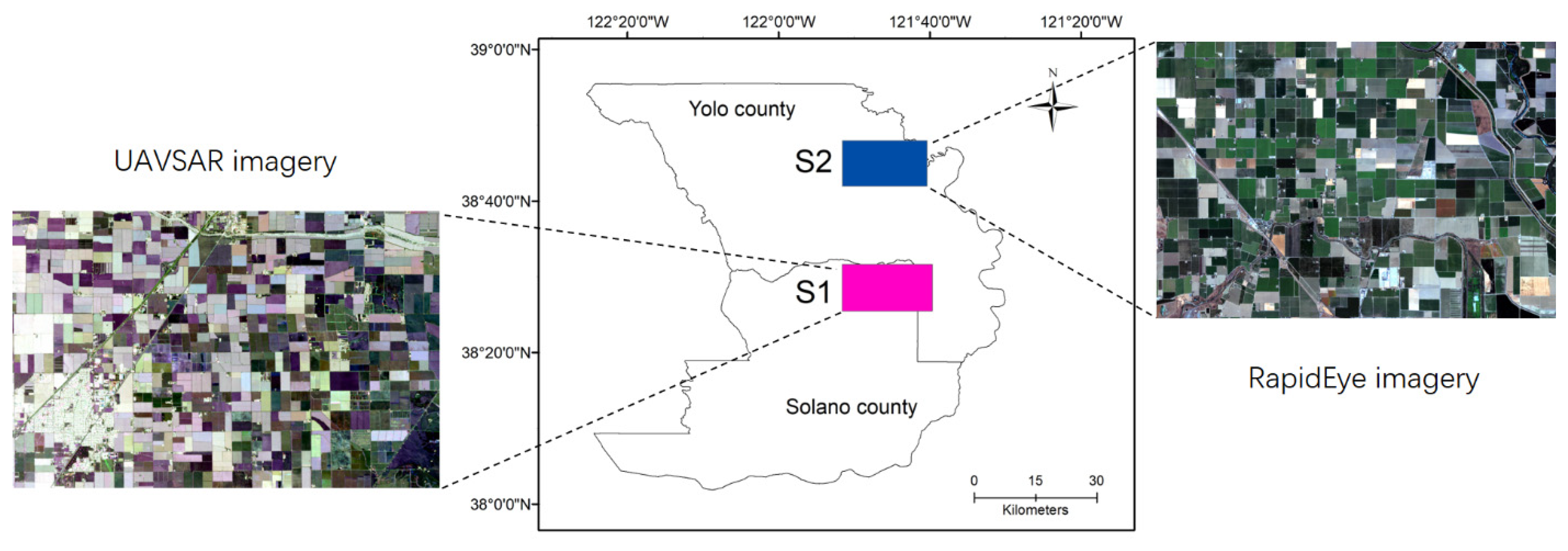
3.1. Study Area and Data

In this research, two typical crop areas (Figure 4), S1 and S2, located in the middle of the Sacramento Valley, in northern California were selected as case study sites. California is considered as a productive agricultural state in the United States, and accounts for about 15% of national receipts for crops [50]. The two study sites are heterogeneous and different from each other in crop composition, thus, being ideal to test remote sensing image classification algorithms. Based on the Crop Data Layer (CDL) produced by the United States Department of Agriculture (USDA) [51], 10 dominant crop classes were found within S1 (

Table 1. Number of collected samples for each crop class over the two study sites.

Study Sites	Crop Class	Number of Objects	Training Sample	Testing Sample	Total Sample
S1	Walnut	31	112	112	224
	Almond	33	110	110	220
	Alfalfa	55	125	125	250
	Hay	26	101	101	202
	Clover	41	110	110	220
	Winter wheat	68	120	120	240
	Corn	45	108	108	216
	Sunflower	47	122	122	244
	Tomato	58	120	120	240
	Pepper	32	106	106	212
S2	Walnut	39	108	108	216
	Almond	45	115	115	230
	Fallow	30	90	90	180
	Alfalfa	35	124	124	248
	Winter wheat	40	116	116	232
	Corn	22	93	93	186
	Sunflower	57	130	130	260
	Tomato	63	141	141	282
	Cucumber	21	93	93	186

), including walnut, almond, alfalfa, hay, clover, winter wheat, corn, sunflower, tomato and pepper, and nine major crop classes (Table 1) in S2, namely walnut, almond, fallow, alfalfa, winter wheat, corn, sunflower, tomato and cucumber.

In S1, the Uninhabited Aerial Vehicle Synthetic Aperture Radar (UAVSAR) image was captured on 29 August 2011 (the peak biomass stage). The UAVSAR, an airborne polarimetric interferometric radar system, is operated in L-band with a wavelength of 23.84 cm [52]. The range and azimuth pixel spacings in single look complex imagery are 1.66 m and 1 m, respectively. The UAVSAR used in S1 is in the GRD format (georeferenced), in which the calibrated complex data were multilooked and projected to the ground coordinate. The data has a fine spatial resolution of 5 m and a spatial extent of 3474 × 2250 pixels. No additional filter algorithms were applied to the image, since multiplicative noise was reduced by the multilook procedure [53]. Three raw linear polarizations (HH, HV and VV), as well as six parameters (stated in Section 2.3.1) from the Cloude-Pottier and Freeman-Durden decompositions, were extracted for crop classification.

In S2, a cloud-free RapidEye image (Level 3A Ortho product) was acquired on 10 July 2016. RapidEye is a constellation of five satellites that are equally spaced in the same orbital plane, producing a ground sampling distance (GSD) of 6.5 m at nadir [54]. The RapidEye imagery used in S2 is Ortho product, with sensor, radiometric and geometric correction using level 1 digital terrain elevation data, was delivered resampled to a spatial resolution of 5 m. The image employed in this research has a spatial extent of 3222 × 2230 pixels and five optical bands, namely blue (440–550 nm), green (520–590 nm), red (630–685 nm), red edge (690–730 nm) and near infrared (760–850). To obtain surface reflectance, the image was atmospherically corrected using the atmospheric and topographic correction method supported by the ERDAS IMAGINE software.

We acquired sample points from the USDA-CDL data by means of stratified random sampling. The CDL data are widely used as a ground reference owing to their very high quality [10,55]. Patches of major crop types in each site were outlined [10] and split randomly into two equal subsets. A 50% subset was for training samples generation, and the other 50% subset for testing samples collection, so as to make sure that training and testing samples come from different crop patches. To acquire enough representative samples, the sample size for each crop class was set at around 200 over the two study sites (Table 1). A total number of 2268 and 2020 samples were acquired for S1 and S2, respectively. Note that 80% of the training samples were used to train individual classification methods and the remaining 20% (validation set) were employed to select the optimal hyper-parameters of the classifiers.

To further test the generalisation of the proposed method, additional scenes of UAVSAR (03 October 2011) at S1 and RapidEye (07 September 2016) at S2 were acquired and preprocessed as described previously. Three linear polarizations (HH, HV and VV) of the UAVSAR and four spectral bands (i.e., blue, green, red, red edge) of the RapidEye were extracted, respectively, for crop classification.

3.2. Model Structure and Parameters

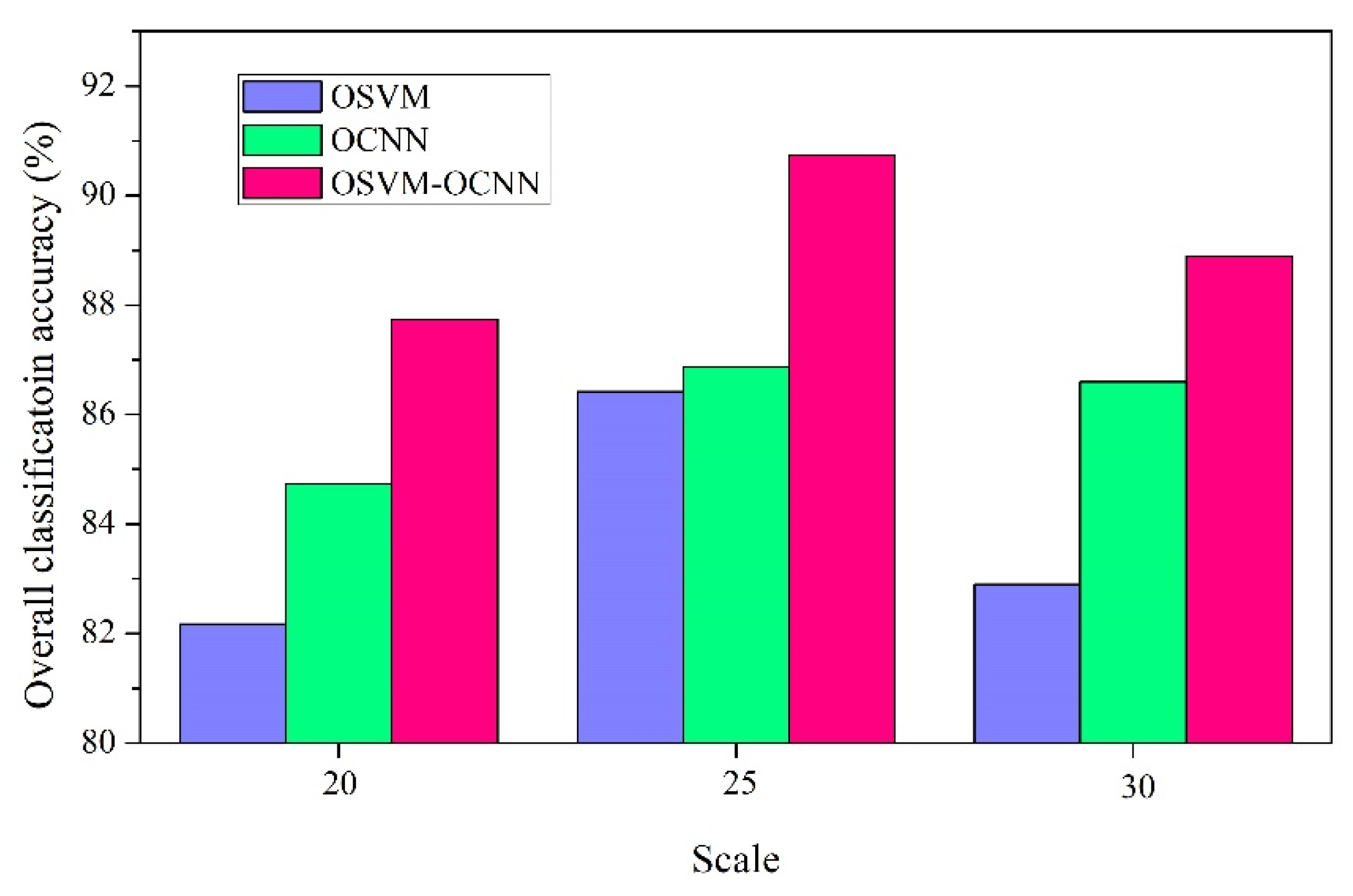
3.2.1. Segmentation Parameter

We implemented the multi-resolution segmentation (MRS) algorithm in the eCognition Developer [56]. Three control parameters, namely, scale, colour/shape and smoothness/compactness, were tuned by means of a systematic trial-and-error process. A relatively small value of the scale parameter was set for a small amount of over-segmentation, thus, assuring the homogeneity of the segmented objects. The optimal combinations of image segmentation parameters over the two study sites are summarised in

Table 2. Parameters used in the multi-resolution segmentation algorithm in the two study sites.

Study Sites	Imagery	Scale	Colour/Shape	Smoothness/Compactness	Number of Objects	Mean Area of Objects (ha)
S1	UAVSAR	25	0.8/0.2	0.3/0.7	4210	4.64
S2	RapidEye	130	0.9/0.1	0.2/0.8	9192	2.95

.

3.2.2. Model Structure and Parameter Settings

The object-based SVM (OSVM) model involves two major parameters that need to be pre-defined, the penalty parameter (C) and the kernel parameter (γ), each of which has been shown to influence model outputs [57]. The former determines the trade-off between model complexity and training error, while the latter controls the shape of the hyperplane. To search for the best parameters for the model, a “grid-search” on C and γ with exponentially growing sequences (i.e., 10-2, 10-1, …, 103) using five-fold cross-validation was performed [49]. The optimal combination of parameters over both study sites was found to be 1000 and 0.1, by which the OSVM delivered the best classification results.

For the object-based CNN (OCNN) model, a range of pre-defined parameters need to be tuned, including the input window size, the number of layers, as well as the number of convolutional filters. The input window size of the OCNN was determined through cross-validation from a series of window sizes {24 × 24, 32 × 32, 40 × 40, 48 × 48, 56 × 56, 64 × 64}, and 40 × 40 and 32 × 32 were found to be the optimal sizes for S1 and S2, respectively. To balance network complexity and generalization ability, the number of network layers was tuned to six (Figure 5) and a 2 × 2 max pooling layer following each convolutional layer was used to further generalise the extracted features. The other parameters were designated as follows: the filter size was 3 × 3 for the convolutional layers (except for the first layer which was 5 × 5); the number of filters in each convolutional layer was 32; the learning rate and the number of epochs were respectively 0.01 and 500 to fully extract high-level features contained in the images. The cross-entropy loss was employed as the objective function. For training the entire network, the mini-batch stochastic gradient descent with a batch size of 20 samples was adopted to minimise the loss function. The CNN was built using Keras library with Tensorflow backend.

3.2.3. Pixel-wise Classifiers and Their Parameters

The RBF SVM model was used for traditional pixel-wise SVM classification. The two control parameters (C and γ) were optimised using a “grid-search” approach as mentioned above [49], and the optimal combination of parameters was found to be 100 and 1.

The traditional pixel-wise CNN also requires a pre-defined series of control parameters. The input window size was selected from {16 × 16, 24 × 24, 32 × 32, 40 × 40 and 48 × 48} and 24 × 24 was found to be the optimal patch size at both the S1 and S2 sites. The number of layers was tuned to six and the number of filters at each convolutional layer was set to 32. The size of convolutional filters was 5 × 5 for the first convolutional layer and 3 × 3 for the other layers, the same as for the OCNN. The learning rate and the maximum number of iterations were designated as 0.01 and 500, respectively.

3.3. Decision Fusion Parameters

A rule-based decision fusion approach was performed based on the OCNN’s prediction probability and the classification results of both OSVM and OCNN models. As mentioned above, the parameter of the decision fusion rules was optimised by a grid search approach through cross-validation. The optimal threshold (α) was found to be 0.98 at S1 and 0.91 at S2, respectively.

3.4. Results and Analysis

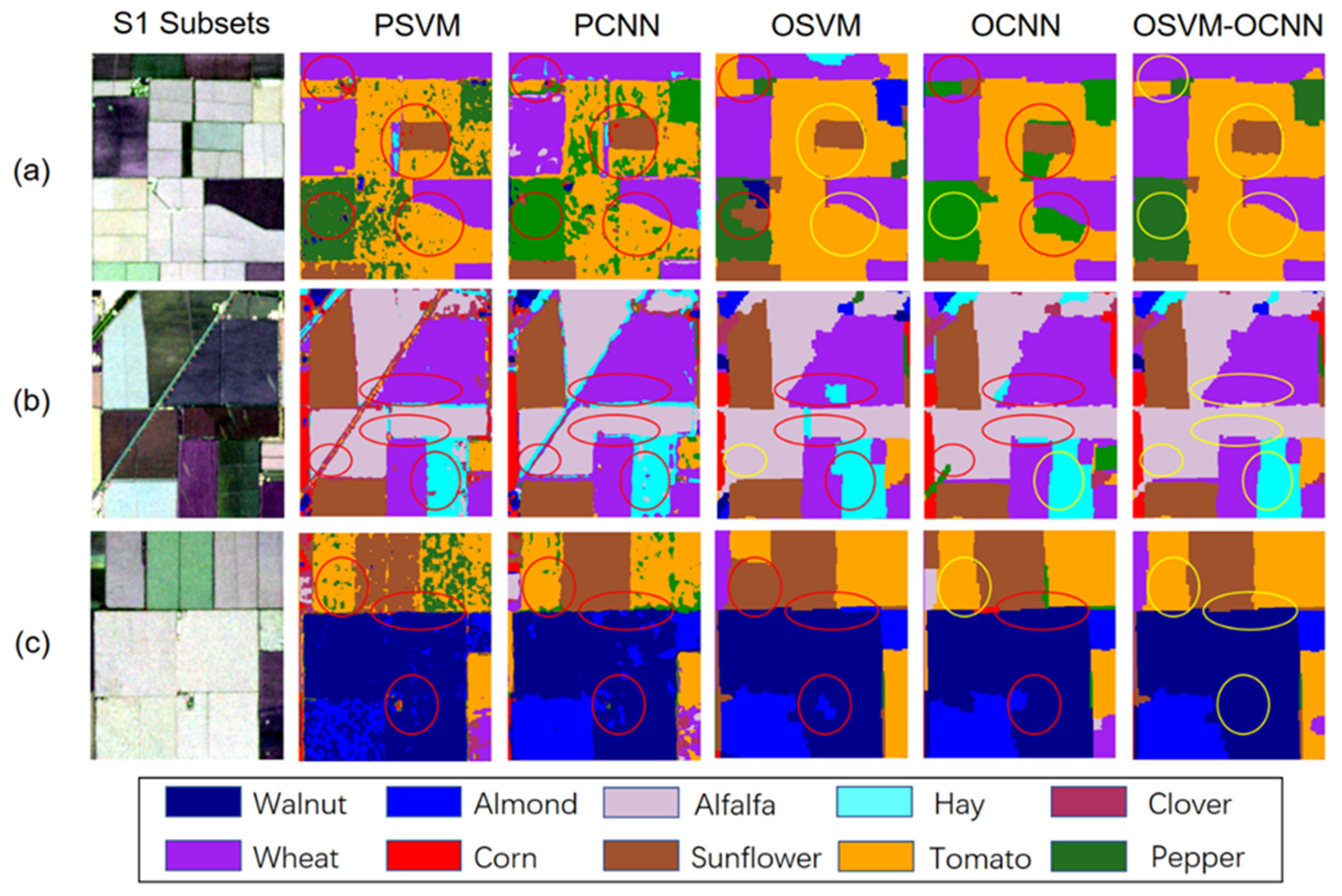
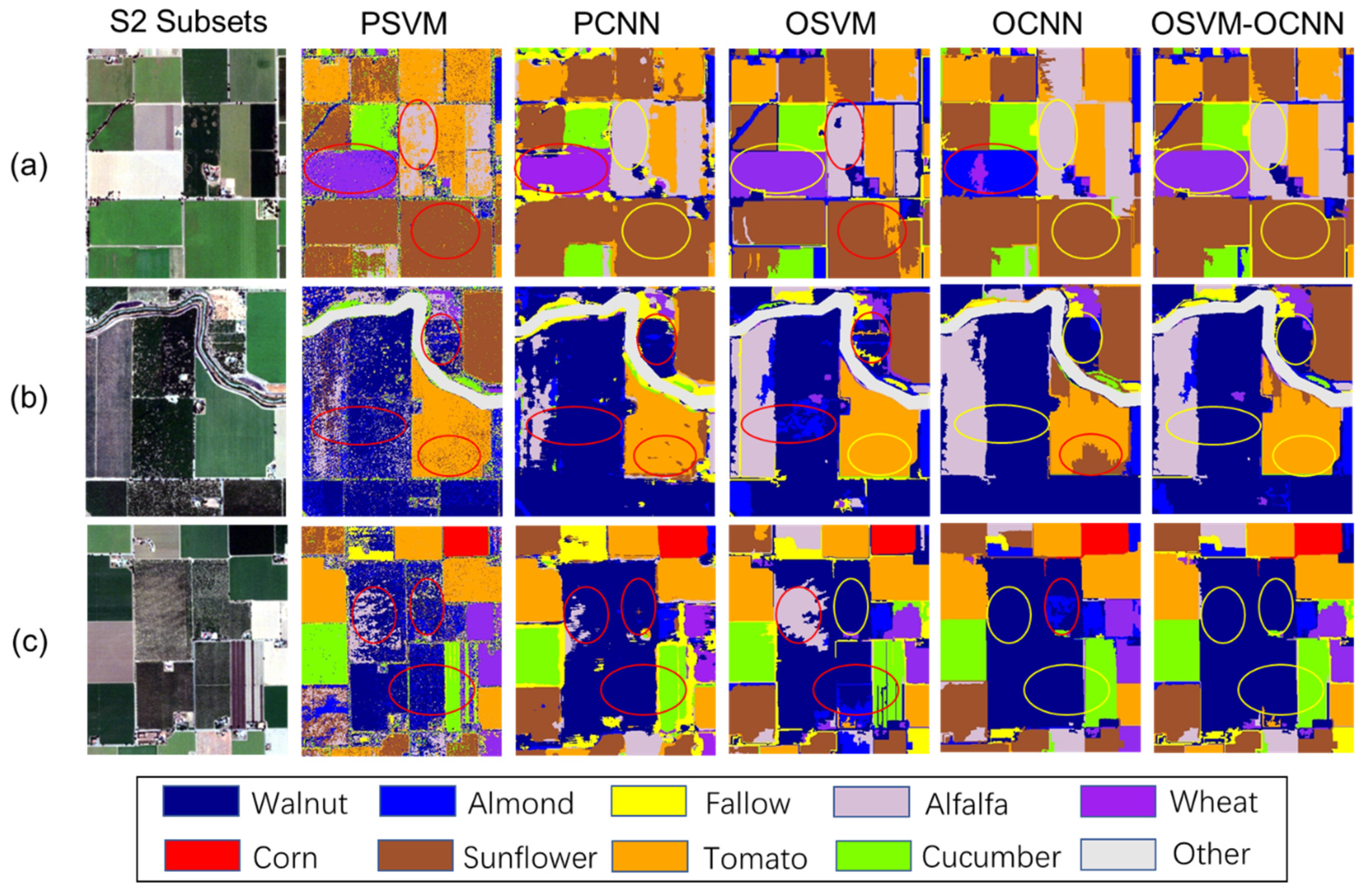
3.4.1. Classification Maps and Visual Assessment

The classification maps achieved by the OSVM-OCNN were examined at both study sites. We compared the new OSVM-OCNN method with its two sub-models (OSVM and OCNN), as well as the PSVM and PCNN. To provide a clear visualization, Figure 6 and Figure 7 illustrate visual inspections of the classification maps using subset images of the two study sites. It is clear that the PSVM achieved undesirable results (salt-and-pepper noise), as demonstrated in Figure 6 and Figure 7. Moreover, tomato and pepper, as well as walnut and almond, were frequently misclassified as each other, as shown in Figure 6a,c. However, the PCNN has certain advantages over the PSVM in discriminating these crop classes with similar spectral characteristics. For example, as illustrated by Figure 6c and Figure 7a, walnut and alfalfa were better distinguished from almond and tomato, respectively, in comparison to the PSVM classifications. Additionally, the salt-and-pepper noise was reduced to some extent due to the use of contextual information. The salt-and-pepper noise still existed in the CNN classifications (especially in the UAVSAR-based CNN classification), and the misclassifications between pepper and tomato and walnut and almond were still present, as illustrated in Figure 6 and Figure 7.

In contrast to the pixel-wise SVM and CNN, the classification maps generated by the object-based SVM and CNN exhibited very smooth visual appearance, and the salt-and-pepper noise was removed, as shown in Figure 6 and Figure 7. The classification of fruit crops (walnut and almond), forage crops (alfalfa and hay) and summer crops (corn, tomato and pepper) was also improved to some extent as shown by the yellow circles in Figure 6 and Figure 7. Specifically, parts of tomato were misclassified by the OCNN, whereas these areas were accurately classified by the OSVM (Figure 6a). In contrast, the OSVM was less accurate than the OCNN when identifying hay and tomato (Figure 6b,c). Similarly, the OSVM was more accurate than the OCNN in identifying wheat and tomato while the OCNN showed certain advantages over the OSVM in discriminating alfalfa, walnut and cucumber (Figure 7).

When checking the classification maps of the OSVM-OCNN, most of the aforementioned misclassifications achieved by OSVM and OCNN were revised while keeping the smoothness of the classifications. For example, the OSVM-OCNN modified the misclassifications of the OSVM for pepper, as shown in Figure 6a, and for sunflower and walnut, as shown by Figure 7, which benefitted from the accurate classification of the OCNN. Moreover, the OSVM-OCNN revised the classification errors of the OCNN for tomato (Figure 6a and Figure 7b) and wheat (Figure 7a). More importantly, some mutual misclassifications between the OSVM and OCNN were effectively resolved. For example, as illustrated in Figure 6b,c, some wheat and walnut patches were misclassified as hay and almond, respectively, in both the OSVM and OCNN classifications; however, they appeared at different places, and nearly all the mislabelled patches were rectified when combining the two classification results using the decision fusion strategy provided in this research.

3.4.2. Classification Accuracy Assessment

In addition to visual assessment, we further investigated the classification accuracy of the proposed OSVM-OCNN and the other benchmark methods, including the PSVM, PCNN, OSVM, and the OCNN over the two study sites.

Table 3. Overall accuracy as well as per-class accuracy achieved by the PSVM, PCNN, OSVM, OCNN and OSVM-OCNN method with the UAVSAR image in S1; the greatest classification accuracy per row is highlighted in bold font.

Crop Type	PSVM	PCNN	OSVM	OCNN	OSVM-OCNN
Walnut	80.91	87.85	84.58	91.89	96.33
Almond	76.56	88.60	86.76	91.15	95.65
Alfalfa	72.51	88.35	84.87	88.26	89.96
Hay	62.56	77.94	76.35	89.00	87.37
Clover	71.68	90.83	91.63	91.16	94.17
Winter wheat	70.13	64.68	83.47	80.49	83.26
Corn	83.82	88.00	89.20	95.89	96.39
Sunflower	69.60	80.46	95.51	85.96	93.62
Tomato	74.89	74.89	89.16	81.27	87.55
Pepper	63.16	70.71	80.18	74.40	83.10
Overall accuracy (OA)	72.75	81.31	86.42	86.86	90.74
Kappa coefficient (k)	0.70	0.79	0.85	0.85	0.90

and

Table 4. Overall accuracy as well as per-class accuracy achieved by the PSVM, PCNN, OSVM, OCNN and OSVM-OCNN method with the RapidEye image in S2; the greatest classification accuracy per row is highlighted in bold font.

Crop Type	PSVM	PCNN	OSVM	OCNN	OSVM-OCNN
Walnut	58.71	79.28	72.95	83.66	84.82
Almond	55.11	63.54	75.34	69.38	79.65
Fallow	61.08	66.36	70.93	70.37	78.82
Alfalfa	67.46	79.83	76.68	78.46	82.35
Winter wheat	79.52	80.70	88.89	83.66	91.92
Corn	96.67	95.19	97.24	98.36	99.46
Sunflower	70.64	83.02	81.66	85.07	87.69
Tomato	75.00	83.51	86.12	84.09	87.91
Cucumber	66.67	79.00	83.33	84.69	87.50
Overall accuracy (OA)	70.20	79.11	81.39	81.68	86.63
Kappa coefficient (k)	0.66	0.76	0.79	0.79	0.85

list the detailed classification accuracy of the methods in both S1 and S2 using the overall accuracy (OA), Kappa coefficient ($\kappa$) and per-class mapping accuracy. As shown in the tables, the OSVM-OCNN acquired the greatest OA of 90.74% at S1 and 86.63% at S2 with $\kappa$ of 0.90 and 0.85, respectively, consistently greater than the OCNN (86.86% and 81.68% OA with $\kappa$ of 0.85 and 0.79, respectively) and OSVM (86.42% and 81.39% with corresponding $\kappa$ of 0.85 and 0.79, respectively). The increase in classification accuracy was much more conspicuous when compared to the pixel-wise classifiers, such as the PCNN (81.31% and 79.11% OA with $\kappa$ of 0.79 and 0.76, respectively) and PSVM (72.75% and 70.20% OA with corresponding $\kappa$ of 0.70 and 0.66, respectively). In addition, a McNemar test developed for pair-wise comparison further demonstrated the proposed OSVM-OCNN achieved significantly increased classification accuracy in comparison with the PSVM and PCNN, as well as the OSVM and OCNN, with z-value = 12.56, 7.44, 4.35 and 4.92 in S1 and z-value = 10.76, 5.63, 6.57 and 4.32 in S2, respectively (

Table 5. McNemar test results for comparing the performance of the five methods over both study sites; bold font indicates that the compared two methods are significantly different at the 95% confidence level.

Study Sites	Classifiers	Mcnemar Test z-Value
		PSVM	PCNN	OSVM	OCNN	OSVM-OCNN
S1	PSVM	-
	PCNN	5.98	-
	OSVM	8.55	3.44	-
	OCNN	9.92	4.58	0.35	-
	OSVM-OCNN	12.56	7.44	4.35	4.92	-
S2	PSVM	-
	PCNN	5.88	-
	OSVM	7.43	1.61	-
	OCNN	7.40	1.80	0.21	-
	OSVM-OCNN	10.76	5.63	6.57	4.32	-

). However, there was no significant difference between the OSVM and OCNN classifications over both study sites despite the OAs of the OCNN being slightly higher than those of the OSVM.

The superiority of the OSVM-OCNN method was also checked with class-wise accuracy assessment (Table 3 and Table 4). As shown in the tables, the OSVM-OCNN achieved the most accurate class-wise classification for most of the crop types in S1 and all types in S2. The largest increase was up to 8.70% for pepper in S1 and 10.27% for almond in S2, when compared with the OCNN. The accuracy increase was also significant for sunflower (7.66%) and tomato (6.28%) in S1 and fallow (8.45%) and winter wheat (8.26%) in S2. In comparison to the OSVM, most crop classes in S1 and all classes in S2 were classified with greater accuracy with the OSVM-OCNN. Specifically, walnut exhibited the greatest increase in accuracy over both study sites, up to 11.75% at S1 and 11.87% at S2, respectively. As for winter wheat, sunflower and tomato in S1, the accuracy of the OSVM-OCNN was slightly less than that of the OSVM without significant differences. The accuracy increase of the OSVM-OCNN tended to be more obvious in comparison to the PSVM and PCNN. Here, the OSVM-OCNN was constantly superior to the PCNN and PSVM at the class-wise level, with the largest increase up to 18.58% and 24.81% for winter wheat and hay in S1 and 16.11% and 26.11% for almond and walnut in S2, respectively.

For the four benchmark methods themselves (i.e., the PSVM, PCNN, OSVM and the OCNN), the OCNN achieved the greatest accuracy, followed by the OSVM and PCNN, while the PSVM was the least accurate. In S1, the two object-based methods (OSVM and OCNN) were significantly more accurate than the two pixel-wise methods (PSVM and PCNN), as demonstrated by the McNemar test (Table 5). In S2, the accuracies of the OSVM and OCNN were significantly greater than that of the PSVM (z = 7.43 and 7.40, respectively), but only slightly (about 2%) greater than that of the PCNN with no significant difference (z = 1.61 and 1.80, respectively). Between the same type of classifiers, it was found that the PCNN performed significantly more accurately than the PSVM (z = 5.98 and 5.88, respectively), while there was no difference between the OSVM and OCNN (z = 0.35 and 0.21, respectively) at both study sites as shown in Table 5.

The proposed OSVM-OCNN method and the other benchmark comparators were also validated using additional scenes of UAVSAR and RapidEye imagery at S1 and S2 study sites. The classification accuracy assessment including the overall accuracy (OA) and Kappa coefficient (k) was summarised in

Table 6. Classification accuracy comparison amongst PSVM, PCNN, OSVM, OCNN and the proposed OSVM-OCNN method using additional UAVSAR and RapidEye imagery.

Imagery	Date	Accuracy	PSVM	PCNN	OSVM	OCNN	OSVM-OCNN
UAVSAR	03/10/2011	OA	57.23%	68.17%	67.37%	68.61%	70.28%
		k	0.52	0.65	0.64	0.65	0.67
RapidEye	07/09/2016	OA	52.77%	68.32%	73.56%	72.77%	76.44%
		k	0.47	0.64	0.70	0.69	0.73

. The OA and k of both study sites are in accordance with the previous experimental results, where the hybrid OSVM-OCNN achieves the greatest OA of 70.28% at S1 and 76.44% at S2, consistently larger than the two sub-modules (OSVM and OCNN), the PCNN, and the PSVM (Table 6). Such coherency of classification accuracy further demonstrates the generalisability of the proposed method.

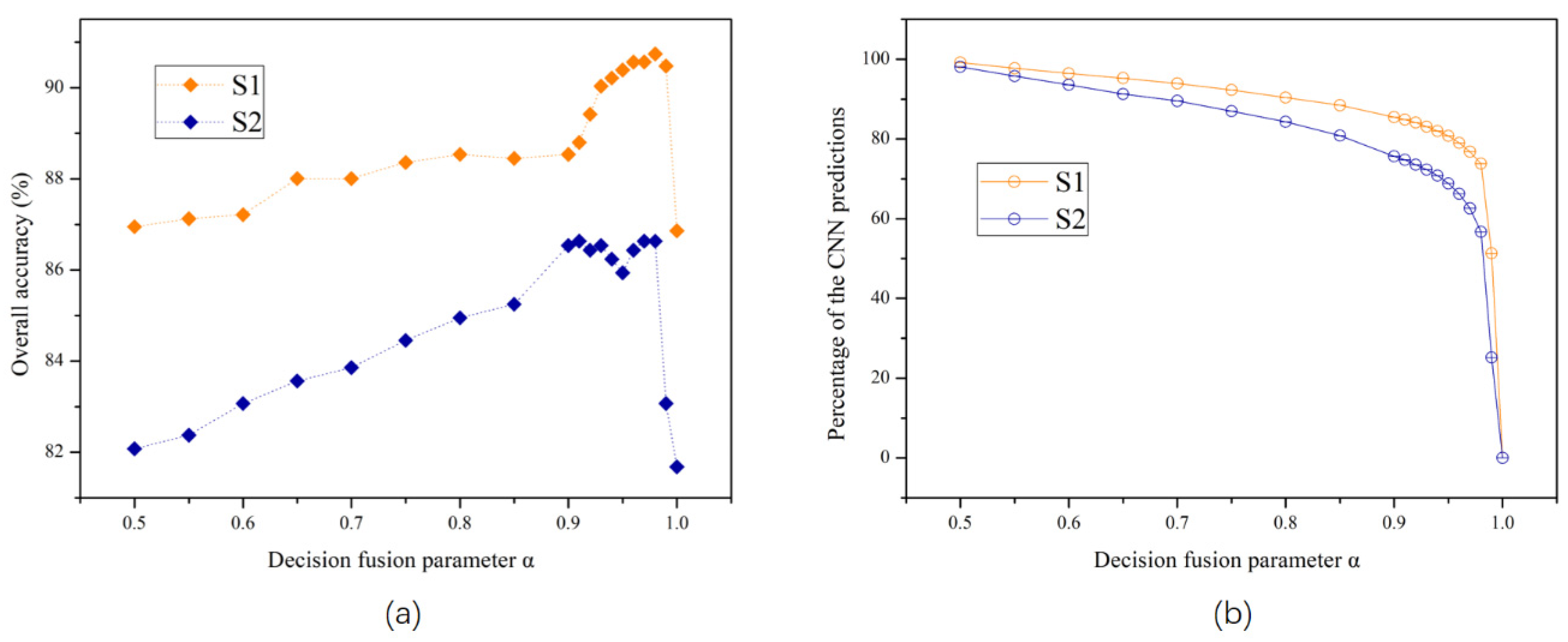
3.5. Influence of the Decision Fusion Parameter

In this subsection, the contribution of the decision fusion parameter (α) (i.e., the prediction probability of the OCNN model) in combining classification results of the two sub-modules (OSVM and OCNN) is investigated (Figure 8). Herein, Figure 8a shows the relations between parameter α and the final classification accuracy (through fusion decision) in S1 (dots in orange) and S2 (dots in blue), respectively; whereas Figure 8b illustrates the area percentage of the OCNN predictions influenced by α in the fused classification map over the two study sites. From Figure 8a, it can be seen that, although there was a difference in accuracy between the two sites resulting from different types of remotely sensed images, the general tendencies in overall accuracy influenced by α over S1 and S2 were similar: the accuracy increased continuously until reaching the maximum accuracy (α = 0.98 in S1 and α = 0.91 in S2), and then tended to decrease with further increases in α. Here, α = 0.98 and α = 0.91 were found to be the optimal decision fusion parameters in S1 and S2, respectively. From Figure 8b, it is clear that when α was small, OCNN predictions dominated the fused outputs with little contribution from the OSVM; in contrary, too large a value for α resulted in a rapid decrease in the area percentage of CNN predictions, leading to a sharp decrease in overall accuracy (Figure 8a). When α approached initially the optimal value, the CNN predictions with low confidence were gradually replaced by accurate SVM predictions, resulting in a rapid increase in accuracy (Figure 8a). The selection of the optimal α value, thus, clearly demonstrates the complementary properties between the two sub-modules by the proposed decision fusion strategy.

4. Discussion

Accurate classification of FSR remotely sensed images is considered a major challenge within the remote sensing community [57]. Combination of different classifiers is an effective means to solve the complex FSR image classification problem, where single classifiers should be as unique as possible, so as to produce different decision boundaries [38]. However, traditional classifier fusion methods by integrating classifiers at the pixel level are unsuitable for processing FSR imagery, given the potential for large amounts of noise (see the salt-and-pepper noise in the PSVM classifications, Figure 6 and Figure 7).

In this research, a novel method (OSVM-OCNN) was proposed for the first time by fusing the outputs of the object-based SVM (OSVM) and CNN (OCNN) at the object level for crop classification from FSR images. The OSVM determines the decision boundaries among classes based completely on the low-level within-object information (e.g., spectral, polarimetric, texture; [24]). In such a manner, the OSVM can identify the objects with salient spectral properties (i.e., light regions on the Figure 3b), but has difficulty handling those objects with similar within-object information (e.g., the misclassifications between two types of forage crops (alfalfa and hay), Figure 6b). This is due mainly to the unavailability of high-level between-object information. In fact, for a large crop parcel, it is normally segmented into several small objects due to the heavy spectral and spatial variations. If only the within-object information is utilised, some of the segmented objects might be misclassified. However, if the between-object (contextual) information is also taken into account, sufficiently representative information can be achieved for the objects, thus markedly increasing the chance of correctly identifying those objects. The OCNN extracts hierarchical features from images via an input window using multiple convolution and pooling operations [24]; thus, both low-level and high-level features are incorporated into the classification process. However, with a fixed input window, the OCNN is incapable of accurately extracting key within-object information of particular objects (e.g., small-sized and linearly shaped objects) due to the mismatch between the observational scale of the OCNN and the scale of the objects themselves. For example, as shown in Figure 3c, the OCNN’s prediction probability of some small-sized objects (usually with distinctive within-object information) tends to be relatively low. In fact, as a state-of-the-art deep learning classifier, OCNN is especially distinguished in representing spatial contextual (i.e., between-object) information, whereas OSVM is superior in extracting within-object information. As a consequence, the shallow-structured OSVM and the deep-structured OCNN have intrinsically complementary characteristics in terms of remotely sensed image classification, as illustrated by Figure 8a. It should be noted that the incorporation of both within- and between-object information is normally necessary to identify and classify complex landscapes. This explains why the proposed hybrid OSVM-OCNN method consistently and significantly outperformed its sub-modules (the OSVM and OCNN) as well as traditional pixel-wise classifiers (the PSVM and PCNN) over both study sites (Table 5, Figure 6 and Figure 7).

Searching for the optimal parameter combination of decision fusion rules is a tedious and time-consuming process [41]. In the proposed OSVM-OCNN, a novel decision fusion strategy was developed to integrate the two sub-models, primarily based on the prediction probability of the OCNN in consideration of its superiority in image classification. That is, the OCNN is regarded as the base classifier, and it is given credit as long the key information of the target object is acquired (i.e., high prediction probability); otherwise, the prediction of the OSVM is trusted. The combination of the two classifiers (OSVM and OCNN), therefore, represents a new rule-based decision fusion strategy that incorporates this key principle. Such a fusion strategy exactly capturing the complementarity between the two sub-modules, even with different types of data (optical and SAR images), is straightforward and efficient in comparison to previous methods (in which two or more parameters are usually employed, e.g., [38,58]), since only one parameter ($\alpha$) is required. Moreover, there are some other parameters that need to be finely tuned, including those used in the sub-modules and image segmentation. The control parameters of the SVM and CNN can be tuned relatively easily according to previous research. In contrast, the parameters of segmentation algorithms are usually hard to determine. In the MRS image segmentation algorithm, the scale parameter is considered the most important, as it directly controls the relative size of the segmented objects. In practice, it is almost impossible to select an optimal scale value that can accurately segment all of the ground patches with the boundaries being retained completely. In practice, a relatively small value is always a preferred alternative (e.g., [24]). By taking the UAVSAR experiment as an example, the impact of segmentation on the overall accuracy of the proposed method was illustrated (Figure 9). It can be seen from the figure that the OSVM-OCNN consistently outperformed the two sub-modules, regardless of how the scale parameter is tuned. The scale parameter selected in this research (i.e., scale = 25) that achieves a small amount of over-segmentation is suitable for crop classification. If the value is too small (e.g., scale = 20 in Figure 9), one crop patch may be partitioned into many very small objects; and if it is too large (e.g., scale = 30 in Figure 9), one segmented object may contain many crop patches. Obviously, both cases exert negative impact on the classification results (Figure 9). Therefore, the segmentation parameters employed in this research by trial and error are relatively optimal. Algorithms that automatically determine segmentation parameters (e.g., [59]) could be integrated into the proposed method in future research.

The proposed hybrid OSVM-OCNN approach achieved promising crop classification results for FSR images. In fact, the proposed method that makes full use of both within-object and between-object feature representations has wide potential applicability for a range of complex classification tasks (e.g., Mangroves, [60]; land use, [38]). The proposed classification method, therefore, provides a general solution to address the complex FSR image-based classification problem. It should be mentioned that the effectiveness of the OCNN, a sub-model of the OSVM-OCNN, is constrained by a so-called optimal (fixed-sized) input window as stated previously. A variable sized input window that adjusts dynamically according to the size of objects, thus, deserves to be introduced to the OCNN. This will be investigated in detail in future research.

5. Conclusions

In this research, a novel hybrid method (OSVM-OCNN) was proposed by fusing a shallow-structured object-based SVM (OSVM) and a deep-structured object-based CNN (OCNN) at the object level for crop classification from FSR imagery. The OSVM has advantages in extracting low-level within-object features, while the OCNN is remarkable in terms of generalising high-level between-object information. The proposed OSVM-OCNN method, thus, captures the complementary characteristics of both the OSVM and OCNN models through a set of rules with only one fusion parameter required. Thus, the two sub-models were combined in a concise and effective manner. We investigated the effectiveness of the proposed method over two study sites with distinctive crop compositions using two types of FSR images (UAVSAR and RapidEye), respectively. The OSVM-OCNN consistently achieved the most accurate classification results in comparison to the two sub-models (i.e., OSVM and OCNN), as well as the standard pixel-wise SVM (PSVM) and CNN (PCNN). Thus, we conclude that the presented OSVM-OCNN method is an effective and efficient approach for accurate crop classification (and classification of other complex landscapes) using FSR remotely sensed images, and it is suitable for different types of FSR remotely sensed images.

References

1. Bastiaanssen, W.G.M.; Ali, S. A new crop yield forecasting model based on satellite measurements applied across the Indus Basin, Pakistan. Agric Ecosyst. Environ. 2003, 94, 321–340. [Google Scholar] [CrossRef]
2. Pena-Barragan, J.M.; Ngugi, M.K.; Plant, R.E.; Six, J. Object-based crop identification using multiple vegetation indices, textural features and crop phenology. Remote Sens. Environ. 2011, 115, 1301–1316. [Google Scholar] [CrossRef]
3. Zheng, B.J.; Myint, S.W.; Thenkabail, P.S.; Aggarwal, R.M. A support vector machine to identify irrigated crop types using time-series Landsat NDVI data. Int. J. Appl. Earth Obs. Geoinf. 2015, 34, 103–112. [Google Scholar] [CrossRef]
4. Ramankutty, N.; Evan, A.T.; Monfreda, C.; Foley, J.A. Farming the planet: 1. Geographic distribution of global agricultural lands in the year 2000. Glob. Biogeochem. Cycles 2008, 22, 1. [Google Scholar] [CrossRef]
5. Wardlow, B.D.; Egbert, S.L.; Kastens, J.H. Analysis of time-series MODIS 250 m vegetation index data for crop classification in the US Central Great Plains. Remote Sens. Environ. 2007, 108, 290–310. [Google Scholar] [CrossRef]
6. Wardlow, B.D.; Egbert, S.L. Large-area crop mapping using time-series MODIS 250 m NDVI data: An assessment for the US Central Great Plains. Remote Sens. Environ. 2008, 112, 1096–1116. [Google Scholar] [CrossRef]
7. Conrad, C.; Colditz, R.R.; Dech, S.; Klein, D.; Vlek, P.L.G. Temporal segmentation of MODIS time series for improving crop classification in Central Asian irrigation systems. Int. J. Remote Sens. 2011, 32, 8763–8778. [Google Scholar] [CrossRef]
8. Foody, G.M. Status of land cover classification accuracy assessment. Remote Sens. Environ. 2002, 80, 185–201. [Google Scholar] [CrossRef]
9. Mulla, D.J. Twenty five years of remote sensing in precision agriculture: Key advances and remaining knowledge gaps. Biosyst. Eng. 2013, 114, 358–371. [Google Scholar] [CrossRef]
10. Li, H.P.; Zhang, C.; Zhang, S.Q.; Atkinson, P.M. Crop classification from full-year fully-polarimetric L-band UAVSAR time-series using the Random Forest algorithm. Int. J. Appl. Earth Obs. 2020. under review. [Google Scholar]
11. Li, H.P.; Zhang, C.; Zhang, S.Q.; Atkinson, P.M. Full year crop monitoring and separability assessment with fully-polarimetric L-band UAVSAR: A case study in the Sacramento Valley, California. Int. J. Appl. Earth Obs. 2019, 74, 45–56. [Google Scholar] [CrossRef]
12. Atkinson, P.M.; Tatnall, A.R.L. Neural networks in remote sensing—Introduction. Int. J. Remote Sens. 1997, 18, 699–709. [Google Scholar] [CrossRef]
13. Lu, D.; Weng, Q. A survey of image classification methods and techniques for improving classification performance. Int. J. Remote Sens. 2007, 28, 823–870. [Google Scholar] [CrossRef]
14. Li, H.P.; Zhang, S.Q.; Zhang, C.; Li, P.; Cropp, R. A novel unsupervised Levy flight particle swarm optimization (ULPSO) method for multispectral remote-sensing image classification. Int. J. Remote Sens. 2017, 38, 6970–6992. [Google Scholar] [CrossRef]
15. Blaschke, T. Object based image analysis for remote sensing. Isprs J. Photogramm. Remote Sens. 2010, 65, 2–16. [Google Scholar] [CrossRef] [Green Version]
16. Vuolo, F.; Neuwirth, M.; Immitzer, M.; Atzberger, C.; Ng, W.-T. How much does multi-temporal Sentinel-2 data improve crop type classification? Int. J. Appl. Earth Obs. Geoinf. 2018, 72, 122–130. [Google Scholar] [CrossRef]
17. Immitzer, M.; Vuolo, F.; Atzberger, C. First Experience with Sentinel-2 Data for Crop and Tree Species Classifications in Central Europe. Remote Sens. 2016, 8, 166. [Google Scholar] [CrossRef]
18. Defourny, P.; Bontemps, S.; Bellemans, N.; Cara, C.; Dedieu, G.; Guzzonato, E.; Hagolle, O.; Inglada, J.; Nicola, L.; Rabaute, T.; et al. Near real-time agriculture monitoring at national scale at parcel resolution: Performance assessment of the Sen2-Agri automated system in various cropping systems around the world. Remote Sens. Environ. 2019, 221, 551–568. [Google Scholar] [CrossRef]
19. Castillejo-Gonzalez, I.L.; Lopez-Granados, F.; Garcia-Ferrer, A.; Pena-Barragan, J.M.; Jurado-Exposito, M.; de la Orden, M.S.; Gonzalez-Audicana, M. Object- and pixel-based analysis for mapping crops and their agro-environmental associated measures using QuickBird imagery. Comput. Electron. Agric. 2009, 68, 207–215. [Google Scholar] [CrossRef]
20. Jiao, X.F.; Kovacs, J.M.; Shang, J.L.; McNairn, H.; Walters, D.; Ma, B.L.; Geng, X.Y. Object-oriented crop mapping and monitoring using multi-temporal polarimetric RADARSAT-2 data. Isprs J. Photogramm. Remote Sens. 2014, 96, 38–46. [Google Scholar] [CrossRef]
21. Rogan, J.; Franklin, J.; Stow, D.; Miller, J.; Woodcock, C.; Roberts, D. Mapping land-cover modifications over large areas: A comparison of machine learning algorithms. Remote Sens. Environ. 2008, 112, 2272–2283. [Google Scholar] [CrossRef]
22. Melgani, F.; Bruzzone, L. Classification of hyperspectral remote sensing images with support vector machines. IEEE Trans. Geosci. Remote Sens. 2004, 42, 1778–1790. [Google Scholar] [CrossRef] [Green Version]
23. Liu, X.L.; Bo, Y.C. Object-Based Crop Species Classification Based on the Combination of Airborne Hyperspectral Images and LiDAR Data. Remote Sens. 2015, 7, 922–950. [Google Scholar] [CrossRef] [Green Version]
24. Zhang, C.; Sargent, I.; Pan, X.; Li, H.P.; Gardiner, A.; Hare, J.; Atitinson, P.M. An object-based convolutional neural network (OCNN) for urban land use classification. Remote Sens. Environ. 2018, 216, 57–70. [Google Scholar] [CrossRef] [Green Version]
25. Chen, Y.S.; Jiang, H.L.; Li, C.Y.; Jia, X.P.; Ghamisi, P. Deep Feature Extraction and Classification of Hyperspectral Images Based on Convolutional Neural Networks. IEEE Trans. Geosci. Remote Sens. 2016, 54, 6232–6251. [Google Scholar] [CrossRef] [Green Version]
26. Zhao, L.L.; Yang, J.; Li, P.X.; Zhang, L.P. Characteristics Analysis and Classification of Crop Harvest Patterns by Exploiting High-Frequency MultiPolarization SAR Data. IEEE J. Sel. Top. Appl. Earth Obs. Remote Sens. 2014, 7, 3773–3783. [Google Scholar] [CrossRef]
27. Walde, I.; Hese, S.; Berger, C.; Schmullius, C. From land cover-graphs to urban structure types. Int. J. Geogr. Inf. Sci. 2014, 28, 584–609. [Google Scholar] [CrossRef]
28. Arvor, D.; Durieux, L.; Andres, S.; Laporte, M.A. Advances in Geographic Object-Based Image Analysis with ontologies: A review of main contributions and limitations from a remote sensing perspective. Isprs J. Photogramm. Remote Sens. 2013, 82, 125–137. [Google Scholar] [CrossRef]
29. Zhang, C.; Sargent, I.; Pan, X.; Li, H.P.; Gardiner, A.; Hare, J.; Atkinson, P.M. Joint Deep Learning for land cover and land use classification. Remote Sens. Environ. 2019, 221, 173–187. [Google Scholar] [CrossRef]
30. LeCun, Y.; Bengio, Y.; Hinton, G. Deep learning. Nature 2015, 521, 436–444. [Google Scholar] [CrossRef]
31. Hinton, G.; Deng, L.; Yu, D.; Dahl, G.E.; Mohamed, A.R.; Jaitly, N.; Senior, A.; Vanhoucke, V.; Nguyen, P.; Sainath, T.N.; et al. Deep Neural Networks for Acoustic Modeling in Speech Recognition. IEEE Signal Process. Mag. 2012, 29, 82–97. [Google Scholar] [CrossRef]
32. Niu, X.X.; Suen, C.Y. A novel hybrid CNN-SVM classifier for recognizing handwritten digits. Pattern Recognit. 2012, 45, 1318–1325. [Google Scholar] [CrossRef]
33. Zhang, K.; Zuo, W.M.; Chen, Y.J.; Meng, D.Y.; Zhang, L. Beyond a Gaussian Denoiser: Residual Learning of Deep CNN for Image Denoising. IEEE Trans. Image Process. 2017, 26, 3142–3155. [Google Scholar] [CrossRef] [PubMed]
34. Cheng, G.; Zhou, P.C.; Han, J.W. Learning Rotation-Invariant Convolutional Neural Networks for Object Detection in VHR Optical Remote Sensing Images. IEEE Trans. Geosci. Remote Sens. 2016, 54, 7405–7415. [Google Scholar] [CrossRef]
35. Langkvist, M.; Kiselev, A.; Alirezaie, M.; Loutfi, A. Classification and Segmentation of Satellite Orthoimagery Using Convolutional Neural Networks. Remote Sens. 2016, 8, 329. [Google Scholar] [CrossRef]
36. Nogueira, K.; Penatti, O.A.B.; dos Santos, J.A. Towards better exploiting convolutional neural networks for remote sensing scene classification. Pattern Recognit. 2017, 61, 539–556. [Google Scholar] [CrossRef] [Green Version]
37. Stoian, A.; Poulain, V.; Inglada, J.; Poughon, V.; Derksen, D. Land Cover Maps Production with High Resolution Satellite Image Time Series and Convolutional Neural Networks: Adaptations and Limits for Operational Systems. Remote Sens. 2019, 11, 1986. [Google Scholar] [CrossRef]
38. Zhang, C.; Pan, X.; Li, H.P.; Gardiner, A.; Sargent, I.; Hare, J.; Atkinson, P.M. A hybrid MLP-CNN classifier for very fine resolution remotely sensed image classification. Isprs J. Photogramm. Remote Sens. 2018, 140, 133–144. [Google Scholar] [CrossRef]
39. Low, F.; Conrad, C.; Michel, U. Decision fusion and non-parametric classifiers for land use mapping using multi-temporal RapidEye data. Isprs J. Photogramm. Remote Sens. 2015, 108, 191–204. [Google Scholar] [CrossRef]
40. Clinton, N.; Yu, L.; Gong, P. Geographic stacking: Decision fusion to increase global land cover map accuracy. Isprs J. Photogramm. Remote Sens. 2015, 103, 57–65. [Google Scholar] [CrossRef]
41. Du, P.J.; Xia, J.S.; Zhang, W.; Tan, K.; Liu, Y.; Liu, S.C. Multiple Classifier System for Remote Sensing Image Classification: A Review. Sensors 2012, 12, 4764–4792. [Google Scholar] [CrossRef] [PubMed]
42. Breiman, L. Bagging predictors. Mach. Learn. 1996, 24, 123–140. [Google Scholar] [CrossRef] [Green Version]
43. Vapnik, V. The Support Vector method of function estimation. In Nonlinear Modeling; Springer: Boston, MA, USA, 1998; pp. 55–85. [Google Scholar]
44. Baatz, M.; Schaepe, A. Multiresolution Segmentation: An Optimization Approach for High Quality Multi-Scale Image Segmentation; Herbert Wichmann Verlag: Heidelberg, Germany, 2000. [Google Scholar]
45. Cloude, S.R.; Pottier, E. An entropy based classification scheme for land applications of polarimetric SAR. IEEE Trans. Geosci. Remote Sens. 1997, 35, 68–78. [Google Scholar] [CrossRef]
46. Freeman, A.; Durden, S.L. A three-component scattering model for polarimetric SAR data. IEEE Trans. Geosci. Remote Sens. 1998, 36, 963–973. [Google Scholar] [CrossRef] [Green Version]
47. Mountrakis, G.; Im, J.; Ogole, C. Support vector machines in remote sensing: A review. Isprs J. Photogramm. Remote Sens. 2011, 66, 247–259. [Google Scholar] [CrossRef]
48. Zhang, S.Q.; Zhang, J.Y.; Li, F.; Cropp, R. Vector analysis theory on landscape pattern (VATLP). Ecol. Model. 2006, 193, 492–502. [Google Scholar] [CrossRef] [Green Version]
49. Hsu, C.; Chang, C.; Lin, C. A Practical Guide to Support Vector Classification; Department of Computer Science and Information Engineering, National Taiwan University: Taipei, Taiwan, 2010. [Google Scholar]
50. California Agricultural Statistic, USDA’s National Agricultural Statistics Service. 2011. Available online: www.nass.usda.gov/ca (accessed on 10 February 2018).
51. USDA NASS, National Agricultural Statistics Service Cropland Data Layer. 2011. Available online: http://nassgeodata.gmu.edu/CropScape (accessed on 13 February 2018).
52. Fore, A.G.; Chapman, B.D.; Hawkins, B.P.; Hensley, S.; Jones, C.E.; Michel, T.R.; Muellerschoen, R.J. UAVSAR Polarimetric Calibration. IEEE Trans. Geosci. Remote Sens. 2015, 53, 3481–3491. [Google Scholar] [CrossRef]
53. Dickinson, C.; Siqueira, P.; Clewley, D.; Lucas, R. Classification of forest composition using polarimetric decomposition in multiple landscapes. Remote Sens. Environ. 2013, 131, 206–214. [Google Scholar] [CrossRef]
54. RapidEye, Satellite Imagery Product Specifications. 2012. Available online: http://www. rapideye.com (accessed on 16 February 2018).
55. Zhong, L.H.; Gong, P.; Biging, G.S. Phenology-based Crop Classification Algorithm and its Implications on Agricultural Water Use Assessments in California’s Central Valley. Photogramm. Eng. Remote Sens. 2012, 78, 799–813. [Google Scholar] [CrossRef]
56. Definiens, A.G. Definiens eCognition Developer 8 Reference Book; Definiens AG: München, Germany, 2009. [Google Scholar]
57. Huang, C.L.; Wang, C.J. A GA-based feature selection and parameters optimization for support vector machines. Expert Syst. Appl. 2006, 31, 231–240. [Google Scholar] [CrossRef]
58. Zhang, C.; Sargent, I.; Pan, X.; Gardiner, A.; Hare, J.; Atkinson, P.M. VPRS-Based Regional Decision Fusion of CNN and MRF Classifications for Very Fine Resolution Remotely Sensed Images. IEEE Trans. Geosci. Remote Sens. 2018, 56, 4507–4521. [Google Scholar] [CrossRef] [Green Version]
59. Schultz, B.; Immitzer, M.; Formaggio, A.R.; Sanches, I.D.A.; Luiz, A.J.B.; Atzberger, C. Self-guided segmentation and classification of multi-temporal Landsat 8 images for crop type mapping in southwestern Brazil. Remote Sens. 2015, 7, 14482–14508. [Google Scholar] [CrossRef]
60. Heumann, B.W. An Object-Based Classification of Mangroves Using a Hybrid Decision Tree-Support Vector Machine Approach. Remote Sens. 2011, 3, 2440–2460. [Google Scholar] [CrossRef]
Figure 1. Flowchart illustrating the presented object-based support vector machine-object-based convolutional neural network (OSVM-OCNN) method with four major steps: (A) image segmentation, (B) model training, (C) model inference and (D) fusion decision.
Remotesensing 11 02370 g001
Figure 2. Two examples to illustrate the convolutional position (green star) of a specific object (highlighted cyan polygon) as well as the corresponding convolutional input window (yellow rectangle); the other segmented patches are delineated by red polygons. (a) and (b) demonstrate a subset of the Uninhabited Aerial Vehicle Synthetic Aperture Radar (UAVSAR) and RapidEye imagery, respectively. Details of the two types of images employed here are provided in Section 3.
Remotesensing 11 02370 g002
Figure 3. (a) A subset of the UAVSAR image (bands VV, HV and HH) used in this paper, (b) the prediction probability generated by the OSVM model, (c) the prediction probability achieved by the OCNN model. Note that the white objects denote high predictive probability, while dark objects represent low probability.
Remotesensing 11 02370 g003
Figure 4. The two study sites S1 and S2 over the agricultural district of the Sacramento Valley, California.
Remotesensing 11 02370 g004
Figure 5. The model structure and parameter settings of the CNN network employed in this research.
Remotesensing 11 02370 g005
Figure 6. Three representative subsets (ac) from the UAVSAR imagery with the corresponding classification maps; the first column shows the UAVSAR images (bands VV, HV and HH), the following columns illustrate the classification maps achieved by the PSVM, PCNN, OSVM, OCNN, and the proposed OSVM-OCNN, respectively; the regions with correct and incorrect classification results were labelled with yellow and red circles, respectively.
Remotesensing 11 02370 g006
Figure 7. Three representative subsets (ac) from the RapidEye imagery with the corresponding classification maps; the first column shows the RapidEye images (bands Red, Green and Blue), the following columns illustrate the classification maps achieved by the PSVM, PCNN, OSVM, OCNN and the proposed OSVM-OCNN, respectively; the regions with correct and incorrect classification results were labelled with yellow and red circles, respectively.
Remotesensing 11 02370 g007
Figure 8. (a) Variation in classification accuracy and (b) area percentage of the CNN predictions in the fused output, plotted against α.
Remotesensing 11 02370 g008
Figure 9. Classification accuracy of the OSVM, OCNN and the proposed OSVM-OCNN based on the multi-resolution segmentation (MRS) image segmentation results achieved with difference scale values.
Remotesensing 11 02370 g009