Nonlocal Tensor Sparse Representation and Low-Rank Regularization for Hyperspectral Image Compressive Sensing Reconstruction

Abstract

Hyperspectral image compressive sensing reconstruction (HSI-CSR) is an important issue in remote sensing, and has recently been investigated increasingly by the sparsity prior based approaches. However, most of the available HSI-CSR methods consider the sparsity prior in spatial and spectral vector domains via vectorizing hyperspectral cubes along a certain dimension. Besides, in most previous works, little attention has been paid to exploiting the underlying nonlocal structure in spatial domain of the HSI. In this paper, we propose a nonlocal tensor sparse and low-rank regularization (NTSRLR) approach, which can encode essential structured sparsity of an HSI and explore its advantages for HSI-CSR task. Specifically, we study how to utilize reasonably the $l_1$-based sparsity of core tensor and tensor nuclear norm function as tensor sparse and low-rank regularization, respectively, to describe the nonlocal spatial-spectral correlation hidden in an HSI. To study the minimization problem of the proposed algorithm, we design a fast implementation strategy based on the alternative direction multiplier method (ADMM) technique. Experimental results on various HSI datasets verify that the proposed HSI-CSR algorithm can significantly outperform existing state-of-the-art CSR techniques for HSI recovery.

1. Introduction

Hyperspectral image (HSI) is a three-dimension data cube by simultaneously capturing the information over two spatial and one spectral dimensions. The abundant spatial-spectral information is able to provide more accurate and reliable signature features on distinct materials, which contributes to various applications such as scene classification [1], object detection [2], environmental monitoring [3], etc. However, due to the large data sizes of HSI, the storage and transmission on limited resource platform become a challenge problem. Although various methods, mainly including wavelet transform [4,5,6], TDLT + KLT [7], DPCM [8] and JPEG2000 [9,10], have been proposed to compress HSI effectively, they treat the HSI as a collection of single band images and neglect the spatial-spectral knowledge redundancy. Thus, how to build rational and powerful HSI compressive reconstruction models is still a worthy research issue.

Recently, the compressive sensing (CS) [11,12,13] theory offers a brand-new field for HSI acquisition or compression, which only needs to capture a small number of incoherent measurements in the imaging stage. Then, the acquired measurements can be employed to reconstruct the whole HSI. For convenient application of CS on HSI, many well-known techniques [14,15,16,17,18,19,20,21,22,23,24,25,26,27,28,29,30,31,32,33,34,35,36,37,38,39,40,41] have been presented to convert an HSI into a sparse signal. Although HSI CS can greatly reduce the resource consumption on imaging, storage and transmission compared with those conventional compression methods, how to reconstruct precisely the HSI from fewer measurements is still a challenging problem.

One of the main concerns to the ill-posed reconstruction problem is to convert HSI into sparse description form via imposing some proper sparsity priors. For example, some effective sparsity terms with $l_0$, $l_1$ and $l_p$ ($0<p<1$) norms [13,14,15,16] have been presented to characterize the sparsity for signal recovery, but those methods neglect the underlying structure information. Regularization-based approaches usually incorporate the prior knowledge into the observation model and develop a united framework [17,18,19,20]. For those methods, one key issue is how to design a proper regularization term to characterize the sparsity of HSI. The works in [21,22,23] mainly consider the sparsity of abundance matrix by the linear unmixing of an HSI, and then HSI CS models are built using spectral unmixing procedures. By introducing structured sparsity across spatial or spectral dimension, Zhang et al. [24,25,26,27,28] extended the compression method based sparse representation/dictionary learning to HSI compression. More recently, Meza et al. [29,30] explored the group sparsity based spatial/spectral redundancy structure to achieve HSI compressive sensing reconstruction (HSI-CSR). The HSI CS model proposed by Golbabaee et al. [31,32,33,34] utilized the piecewise smooth structure to explain the underlying gradient sparsity of an HSI. However, as those techniques depict the HSI sparsity in vector space, the description form of sparsity is treated as one vector without considering its multidimensional structure. It will inevitably induce losses and distortions of useful structure information.

Tensor-based HSI-CSR approaches can improve remarkably the HSI recovery quality, since the existing methods jointly take into account the spatial-spectral information, and reduce the losses and distortions caused by HSI reshaping [35,36,37,38,39,40,41,42,43,44]. Karami et al. [35,36] exploited discrete wavelet transform and Tucker decomposition (DWT-TD) to encode the spatial-spectral information of HSI. The core idea behind those techniques is first to use DWT to effectively separate an HSI into different sub-images, and then to apply TD on the DWT coefficients of HSI bands to compact the energy of sub-images. Zhang et al. [37,38] compressed an HSI to the core tensor and the HSI could be reconstructed by the multi-linear projection of the factor matrices. Those methods only consider an HSI as a whole 3D tensor while they are short of more potent constraints on spatial-spectral structure of an HSI. Yang [39] employed nonlinear tensor sparse representation to recover an HSI from small number of measurements, and some training examples are required. Wang [40] used the global spatial-spectral correlation and local smoothness properties underlying in an HSI to enhance the HSI-CSR task, in which the tensor Tucker decomposition and 3-D total variation jointly characterize the sparsity of an HSI. Du [41] proposed a patch-based low-rank tensor decomposition for HSI-CSR algorithm that combined the nonlocal similarity across the spatial domain and the low-rank property over spectral domain in a united framework.

Although methods reported in [37,38,40,41] are considerably effective for HSI-CSR compared with vector based approaches, it is difficult to estimate the accurate rank under tensor decomposition and further acquire unique decomposition. Thus, the methods based on tensor decomposition cannot provide an elaborate characterization on spatial-spectral information in HSI-CSR problem. In [42,43], this reasonable usage of the global correlation across spectrum (GCS) and nonlocal self-similarity over space (NSS) prior knowledge have led to quite powerful HSI denoising algorithms, and the effectiveness of GCS and NSS for HSI-CSR has not been reported in the public literature. Such facts inspire us to solve the challenging HSI-CSR problem by the structured sparsity based on GCS and NSS in this paper, and a unified framework combining nonlocal tensor sparse representation and low-rank regularization is proposed for HSI-CSR, as shown in Figure 1. The main contributions of this paper are listed as follows.

• To the best of our knowledge, we are the first to exploit GCS and NSS to construct the nonlocal structure sparsity of HSI that is a faithfully structured sparsity representation form for HSI-CSR task.
• For each cube that is formed by grouping nonlocal similar cubes, the tensor representation based on tensor sparse and low-rank approximation is introduced to encode the intrinsic spatial-spectral correlation.
• The HSI-CSR task is treated as an optimization problem; we resort to alternative direction multiplier method (ADMM) [44] to solve it.

A preliminary version of this work has appeared in [45], which presents the basic approach. In [45], we established the nonlocal structured sparsity from the perspective of the tensor low-rank property, which adopts the two most commonly used tensor low-rank representation forms: tensor low-rank approximation and tensor low-rank decomposition. In this paper, we depict the nonlocal structured sparsity via the tensor low-rank approximation and sparse representation. Although the tensor low-rank decomposition and sparse representation are derived from the Tucker decomposition model, the former needs to preset the ranks along all dimension while the latter introduces an $l_1$-based sparse term on core tensor. In practical application, the latter possesses the reliable capability to represent the high-dimension data by mitigating the tensor rank overfitting or underfitting. In addition, this paper adds: (1) the detailed background of HSI-CSR; (2) the theoretical analysis of NTSRLR; and (3) additional HSI-CSR experiments.

The remainder of this paper is organized as follows. Section 2 introduces the tensor notations and operations commonly used in this paper, and background of CS. In Section 3, a novel algorithm for HSI-CSR based on the NTSRLR model is proposed. Section 4 demonstrates the results of extensive experiments and Section 5 draws the conclusion.

2. Notations and Background of HSI-CS

2.1. Notations

Throughout the paper, we denote scalars, vectors, matrices and tensors by non-bold letters, bold lower case letters, bold upper case letters and calligraphic upper case letters, respectively. Besides, we introduce some necessary notations and preliminaries about tensor as follows. A tensor of order N, which corresponds to a N-dimensional data array, is denoted as $\mathcal{X}\in \mathbb{R}{}^{I_1\times \cdots \times I_n\times \cdots \times I_N}$. Elements of $\mathcal{X}$ are denoted as $a_{i_1\cdots i_n\cdots i_N}$, where $1\le i_n\le I_n$. Definitions of tensor terminologies in the paper follow exactly the same description in [46]. Denote ${\parallel \mathcal{X}\parallel }_F=〈\mathcal{X},\mathcal{X}〉{\left({\sum }_{i_1{i}_2,\dots ,i_N}{|a_{i_1{i}_2,\dots ,i_N}|}^2\right)}^{1/2}$, ${∥\mathcal{X}∥}_1={\sum }_{i_1{i}_2,\dots ,i_N}\left|a_{i_1{i}_2,\dots ,i_N}\right|$ and ${∥\mathcal{X}∥}_0$ as the F-norm, $l_1$ norm and $l_0$ norm of a tensor $\mathcal{X}$, respectively. ${∥\mathcal{X}∥}_0\le K$ means that K is the number of non-zero entries of $\mathcal{X}$. It is convenient to unfold a tensor into a matrix during the algorithm. The “unfold" operation along the mode-n on a tensor $\mathcal{X}$ is defined as $\mathrm{unfold}{}_n\left(\mathcal{X}\right):=X_{\left(n\right)}\in \mathbb{R}{}^{I_n\times (I_1\times \cdots \times I_{n-1}{I}_{n+1}\times \cdots \times I_N)}$, and its opposite operation “fold" is defined as $\mathrm{fold}{}_n\left(X_{\left(n\right)}\right):=\mathcal{X}$. The Kronecker product of matrices $A\in \mathbb{R}{}^{I\times J}$ and $B\in \mathbb{R}{}^{K\times L}$ is a matrix of size $IK$×$JL$, denoted by $A\otimes B$. The multiplication of a tensor $\mathcal{X}$ with a matrix $Y\in \mathbb{R}{}^{I_k\times J_k}$ on mode-k is denoted by $\mathcal{X}{\times }_{k}Y=\mathcal{Z}$, which also can be defined in terms of mode-k unfolding as $Z_k=Y{X}_k$.

Definition 1.

(Tucker decomposition) [46]: The Tucker decomposition form of a tensor $\mathcal{X}$ is:

$$\mathcal{X}=\mathcal{G}{\times }_1{\mathrm{U}}_1{\times }_2\cdots {\times }_N{\mathrm{U}}_{\mathrm{N}}$$

(1)

where $\mathcal{G}\in \mathbb{R}{}^{J_1\times J_2\times \cdots \times J_N}$ is the core tensor and it reflects the interaction between components along different modes, and ${\mathrm{U}}_n\in \mathbb{R}{}^{I_n\times J_n}$ is the orthogonal factor matrix in each mode. Thus, we can achieve the k-unfolding form of Tucker decomposition in Equation (1)

$$X^{\left(n\right)}={\mathrm{U}}_{\mathrm{n}}{G}^{\left(n\right)}({\mathrm{U}}_{\mathrm{N}}\otimes \cdots \otimes {\mathrm{U}}_{\mathrm{n}+1}\otimes {\mathrm{U}}_{\mathrm{n}-1}\otimes \cdots \otimes {\mathrm{U}}_1)$$

(2)

2.2. Background of HSI-CS

For a given HSI $\mathcal{X}\in \mathbb{R}{}^{W\times H\times S}$ ($W\times H$ spatial resolution and S spectral bands), $x\in \mathbb{R}{}^{WHS}$ denotes the vector form of $\mathcal{X}$. Let $N=WHS$, then the compressive measurement $y\in \mathbb{R}{}^M$ can be obtained from the following CS model:

$$y=\Phi x$$

(3)

where $\Phi \in \mathbb{R}{}^{M\times N}(M<N)$ denotes the compressive operator. The CS theory indicates that a sufficiently sparse signal x can be exactly reconstructed from only a few observation y when the compressive operator $\Phi$ satisfies the restricted isometry property (RIP) [11]. Under the RIP, the ill-posed recovery problem can be formulated into following form by pursuing the sparsest signal x, i.e.,

$$x=\underset{x}{min}{\parallel x\parallel }_0,\mathrm{s}.\mathrm{t}.y=\Phi x$$

(4)

where ${\parallel ·\parallel }_0$ denotes $l_0$ norm as a sparsity constraint. However, the $l_0$ norm minimization in Equation (4) is combinatorially NP-hard and unstable with the noise. For this reason, a feasible strategy is to replace nonconvex $l_0$ norm as a convex $l_1$ counterpart [15,47] as follows:

$$x=\underset{x}{min}{\parallel x\parallel }_1,\mathrm{s}.\mathrm{t}.y=\Phi x$$

(5)

The optimization for above $l_1$-minimization CS problem can resort to iterative shrinkage algorithm [48] and Bregman Split algorithm [49].

Since an HSI can be sparsely represented in a certain domain, many CS models have been proposed for an HSI. Zhang et al. [21,22,23] unmixed the HSI into a spatially sparse abundance matrix with an endmember matrix. Meza et al. [29,30,31] extracted the spatial/spectral redundancy structure and then applied the group sparsity constraint. Golbabaee [34] used a wavelet basis to transform the HSI into a sparse matrix, and then adopted the low-rankness and $l_1$ norm to jointly encode sparsity of the matrix. Zhang et al. [37,38] depicted the sparsity of an HSI in the core tensor domain, instead of reshaped vector domain. Further works [39,40,41] employ the sparse tensor decomposition to characterize sparsity of an HSI. However, those sparsity constraint terms are incapable of capturing the underlying structure in an HSI or handling the unwanted noise and artifacts in the CSR procedure. In our method, we try to cope with those problems by introducing more refined prior knowledge of an HSI to perfectly promote HSI-CSR performance.

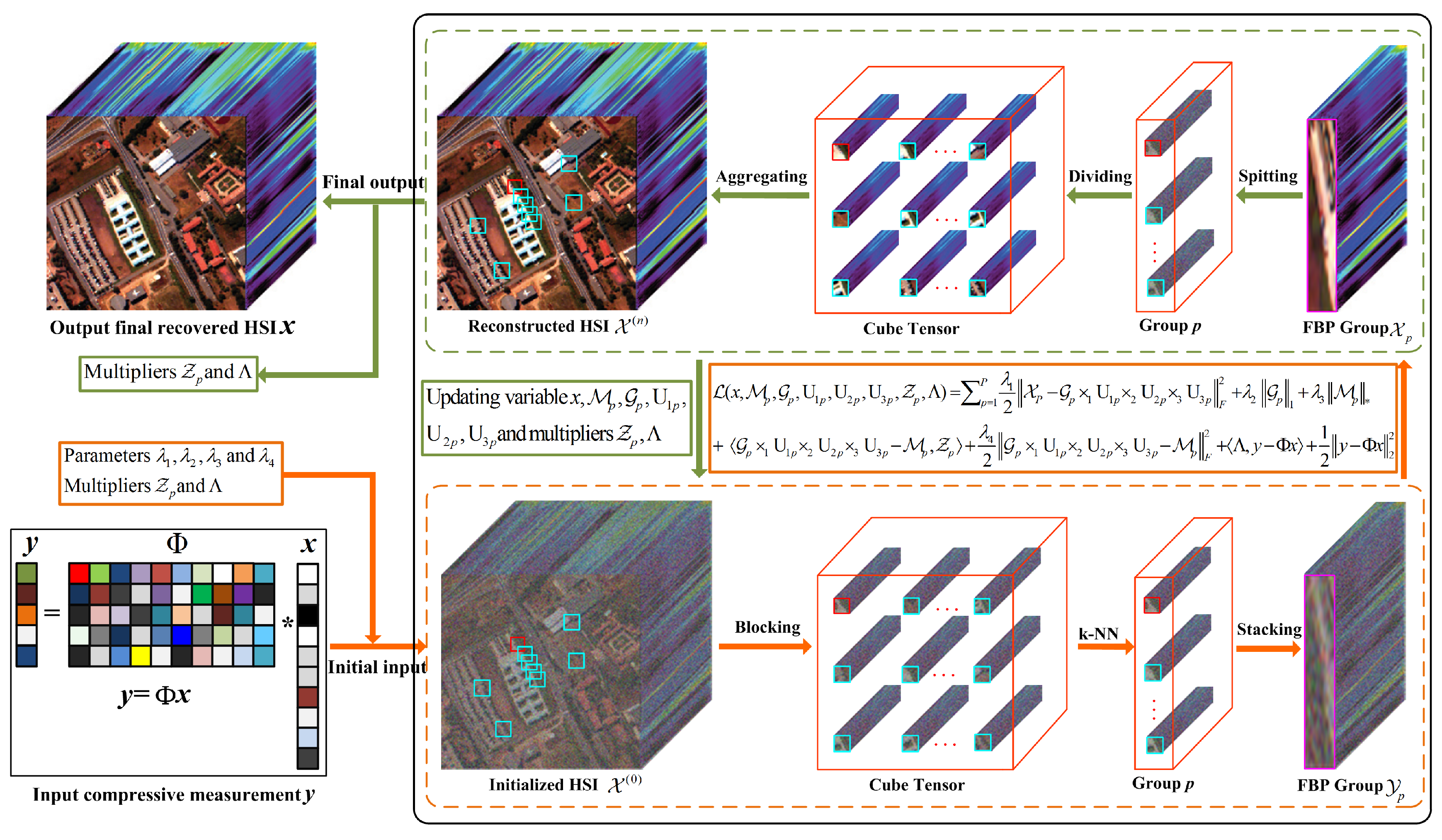
3. The Proposed HSI-CSR via NTSRLR

Structured sparsity is of great importance to the HSI-CSR model that often reveals the rich self-repetitive structures over spatial domain and the highly correlated bands across the spectral domain. Several previous works exploiting nonlocal prior have indicated that the structured sparsity based on nonlocal self-similarity is fairly effective for image restoration [18,19]. However, the research works in HSI-CSR fields have not been documented. In this paper, we present a unified framework for HSI-CSR using the structured sparsity via nonlocal tensor sparse representation and low-rank approximation.

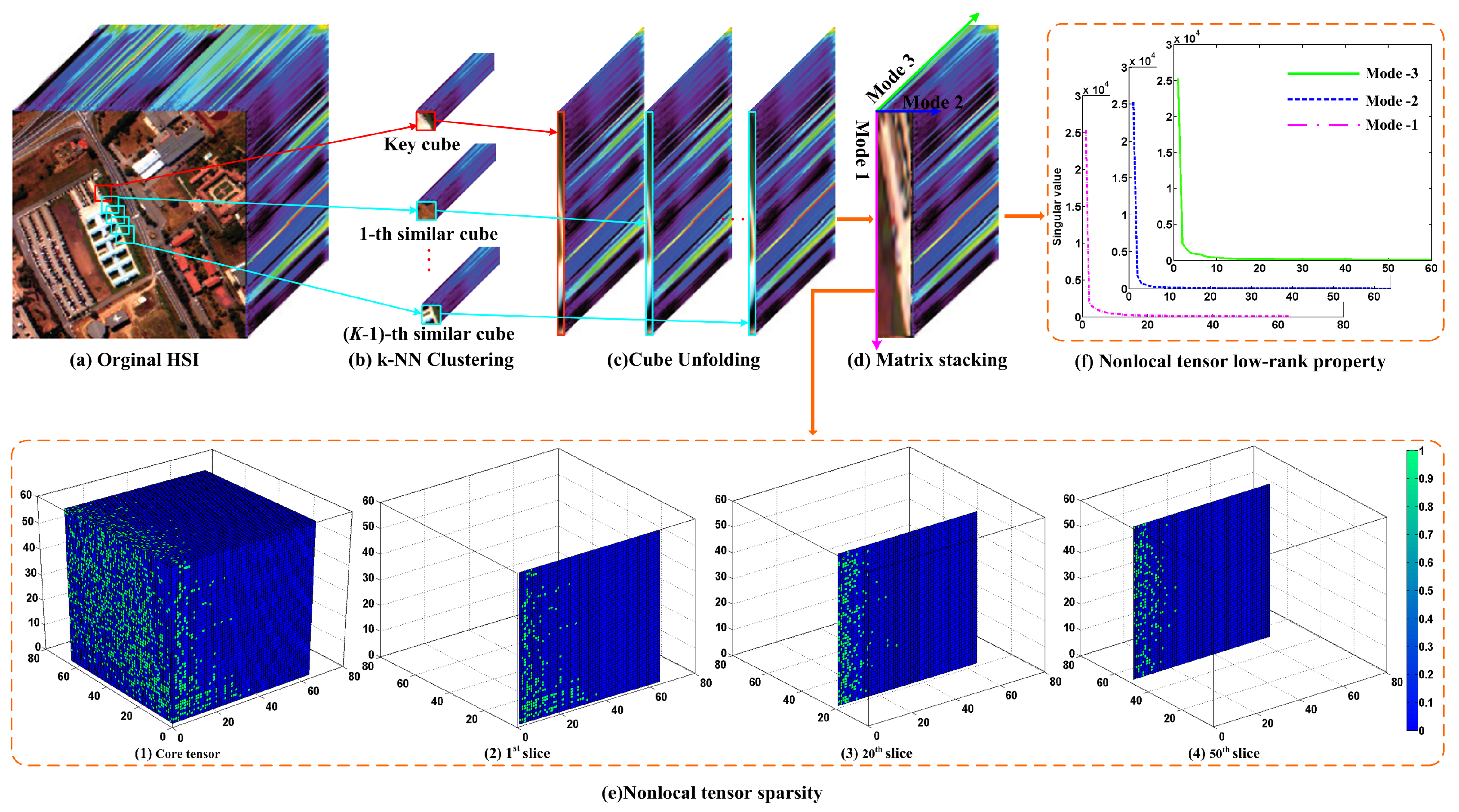
3.1. Non-Local Tensor Formula for Structure Sparsity

The proposed regularization model for structured sparsity consists of two steps: cube grouping for characterizing GCS and NSS and tensor formulation for sparsity enforcement.

3.1.1. Non-Local Structure Sparsity Analysis

Concerning the GCS and NNS underlying an HSI, we provide an analysis for nonlocal tensor sparsity and low-rankness, as illustrated in Figure 2. To begin with, for an initial third-order tensor HSI $\mathcal{X}\in \mathbb{R}{}^{W\times H\times S}$ (e.g., PaviaU dataset), we divide the HSI into a group of 3D full-band cubes (FBC) ${\left\{{\mathcal{P}}_{i,j}\right\}}_{1\le i\le W-w+1,1\le j\le H-h+1}\in {\mathbb{R}}^{w\times h\times S}(w<W,h<H)$ with overlaps. For the exemplar cube ${\mathcal{P}}_{i,j}$ of size 8 × 8 × 60 located at spatial position $(i,j)$ in Figure 2a marked in red, we first search K-1 (here, we set K = 80) similar cubes by k-NN within a local window (e.g., 70 × 70), shown as k-NN clustering in Figure 2b. Then, to avoid destroying the high spectral correlation, we unfold a series of 3D cubes into corresponding 2D matrices along the spectral modes (Figure 2c), and obtain a new third-order tensor ${\mathcal{Y}}_p$ of size 64 × 80 × 60 by stacking a series of similar items (Figure 2d), where $p=1,\dots P$, and P denotes the group number. Such constructed third-order tensor simultaneously employ the spatial local sparsity (mode-1), the non-local similarity between cubes (mode-2) and strong spectral correlation (mode-3). The outcome of such arrangement maximizes the benefit from nonlocal tensor representation form. Next, we give a visual interpretation for the nonlocal tensor sparsity and low-rank property.

First, by Tucker decomposition for a nonlocal similar cube group from PaviaU dataset, Figure 2e shows the location of singular values in the core tensor, where redder and bluer colors of elements represent large values and smaller values, respectively. To further understand the sparsity of tensor core, Figure 2(e2)–(e4) present three typical slices of core tensor. It is easy to find that the core tensor satisfies sparse property, with 82.59% of its elements being zeroes. Second, the low-rank analysis is performed along its local spatial, nonlocal spatial, and global spectral modes, as shown in Figure 2f. Evidently, the decaying trends of singular values on three curves (pink, blue and green curves correspond to local spatial, nonlocal spatial, and global spectral modes, respectively) indicate there are strong correlations in the three modes. Comparatively, the decaying trend of the curve in mode-2 is most drastic, which is consistent with the nonlocal spatial low-rank theory of an HSI given in [50]. According to the definition of the accumulation energy ratio (Aer) of top k singular values in [50], we calculate Top 10 singular values of three modes and attain the Aers of 0.8029, 0.9031 and 0.8186. The quantitative values (i.e., Aers) also indicate that each cube by grouping nonlocal similar cubes can possess strong low-rank correlation along the mode-2.

3.1.2. Non-Local Structure Sparsity Modeling

In Figure 2f, we can observe that the formed FBCs possess the low-rank property, and a tractable strategy is to use the mode-n rank $(r_1,\dots ,r_n)$ to estimate tensor rank by Tucker decomposition [46]. For an Nth-order tensor $\mathcal{X}$, the Tucker rank is defined as $\mathrm{rank}\left(\mathcal{X}\right):=[\mathrm{rank}\left(X_{\left(1\right)}\right),\mathrm{rank}\left(X_{\left(2\right)}\right),\dots ,\mathrm{rank}\left(X_{\left(N\right)}\right)]$, where $X_{\left(i\right)}$ is the mode-i unfolding of $\mathcal{X}$ [51]. Motivated by the practical applications that the nuclear norm is the convex envelope of the matrix rank within the unit ball of the spectral norm, further tensor nuclear norm, ${∥\mathcal{X}∥}_{*}={\sum }_{n=1}^N{{\alpha }_n∥X_{\left(n\right)}∥}_{*}$ is defined as weighting the unfolding matrix nuclear norm along each mode. Thus, we resort to the following relaxation form for each ${\mathcal{X}}_p$ to characterize the low-rank property based on GCS and NSS:

$$\mathcal{L}\left({\mathcal{X}}_p\right)={\sum }_i^3{\alpha }_i\parallel {{\mathcal{X}}_p}_{\left(i\right)}{\parallel }_{*}$$

(6)

where $\parallel {\mathcal{X}}_{p\left(i\right)}{\parallel }_{*}={\sum }_{k=1}^{min(m,n)}{\sigma }_k\left({\mathcal{X}}_{p\left(i\right)}\right)$ denotes the nuclear norm of matrix ${\mathcal{X}}_{p\left(i\right)}$ of size $m\times n$.

In practice, ${\left\{{\mathcal{Y}}_p\right\}}_{p=1}^P$ may contain some noise, the data ${\mathcal{Y}}_p$ can be modeled as: ${\mathcal{Y}}_p={\mathcal{X}}_p+{\mathcal{W}}_p$, where ${\mathcal{X}}_p$ and ${\mathcal{W}}_p$ denote the low-rank component and the noise component, respectively. Hence, we can estimate the low-rank tensor ${\mathcal{X}}_p$ via the following optimization problem:

$${\mathcal{X}}_p=\underset{{\mathcal{X}}_p}{min}\mathcal{L}\left({\mathcal{X}}_p\right),\mathrm{s}.\mathrm{t}.{∥{\mathcal{Y}}_p-{\mathcal{X}}_p∥}_F^2\le \epsilon$$

(7)

where $\epsilon$ is associated with the noise level. The model in Equation (7) is similar to the matrix cases in [18], the difference primarily reflected in that we consider the combination with the correlations along local-nonlocal spatial modes and spectral mode, and measure the low-rankness of a third-order tensor ${\mathcal{X}}_p$ by a weighted sum of the rank along each unfolding. Besides, considering the strong nonlocal spatial low-rankness along mode-2 than two other modes, we set a larger weight for mode-2 in our experiments.

In addition, as shown in Figure 2e, we give a detailed analysis for another notable representation form for the sparsity prior based on tensor sparse decomposition, which suggests that we can depict the structured sparsity of an HSI from the perspective of core tensor. Some pioneering works are presented in [42,43,52,53,54]. Here, we draw attention to the structured sparsity formulation of an HSI under tensor sparse representation framework, thus each third-order tensor ${\mathcal{X}}_p$ can be approximated by following problem:

$$\begin{array}{c}\hfill \underset{{\mathcal{G}}_p,{\mathrm{U}}_{1p},{\mathrm{U}}_{2p},{\mathrm{U}}_{3p}}{min}\mathcal{S}\left({\mathcal{G}}_p\right),\mathrm{s}.\mathrm{t}.{\mathcal{X}}_p={\mathcal{G}}_p{\times }_1{\mathrm{U}}_{1p}{\times }_2{\mathrm{U}}_{2p}{\times }_3{\mathrm{U}}_{3p},{\mathrm{U}}_{ip}^T{\mathrm{U}}_{ip}=I(i=1,2,3)\end{array}$$

(8)

where ${\mathrm{U}}_{1p},{\mathrm{U}}_{2p}$, and ${\mathrm{U}}_{3p}$ are factor matrices and $\mathcal{S}\left({\mathcal{G}}_p\right)$ is sparse constraint term, and we assume $\mathcal{S}\left({\mathcal{G}}_p\right)={∥{\mathcal{G}}_p∥}_0$ as suggested in [42,43,52]. However, the optimization problem based on $l_0$ constraint deduced by Equation (8) is non-convex, the research in [53,54] further relaxes the $l_0$-based core sparsity to $l_1$ case as $\mathcal{S}\left({\mathcal{G}}_p\right)={∥{\mathcal{G}}_p∥}_1$. The convex optimization problem corresponding to $l_1$ case can be represented in Lagrangian form as following:

$$\begin{array}{c}\hfill \underset{{\mathcal{G}}_p,{\mathrm{U}}_{1p},{\mathrm{U}}_{2p},{\mathrm{U}}_{3p}}{min}\frac{{\lambda }_1}{2}{∥{\mathcal{X}}_p-{\mathcal{G}}_p{\times }_1{\mathrm{U}}_{1p}{\times }_2{\mathrm{U}}_{2p}{\times }_3{\mathrm{U}}_{3p}∥}_F^2+{\lambda }_2{∥{\mathcal{G}}_p∥}_1,\mathrm{s}.\mathrm{t}.{\mathrm{U}}_{ip}^T{\mathrm{U}}_{ip}=I(i=1,2,3)\end{array}$$

(9)

where ${\lambda }_1$ and ${\lambda }_2$ are the trade-off parameters. Essentially, all factor matrices are orthogonal dictionaries along local–nonlocal spatial modes and spectral mode. It can be seen that the tensor sparse representation model explores the GCS and NSS of HSIs in different dimensions by adaptive multi-dictionaries learning. Compared with the matrix sparse representation technique [19,20], the advantage of tensor modeling is that it not only characterizes the spatial-spectral correlation but also the correlation over nonlocal similar cubes in an HSI.

3.2. Proposed Model

Based on the previous analysis, we now derive the following model for solving the HSI-CSR problem:

$$\begin{array}{cc}\hfill \underset{x,{\mathcal{G}}_p,{\mathrm{U}}_{1p},{\mathrm{U}}_{2p},{\mathrm{U}}_{3p}}{min}{\sum }_{p=1}^P& \frac{{\lambda }_1}{2}{∥{\mathcal{X}}_p-{\mathcal{G}}_p{\times }_1{\mathrm{U}}_{1p}{\times }_2{\mathrm{U}}_{2p}{\times }_3{\mathrm{U}}_{3p}∥}_F^2+{\lambda }_2\mathcal{S}\left({\mathcal{G}}_p\right)+{\lambda }_3\mathcal{L}\left({\mathcal{X}}_p\right),\hfill \\ & \mathrm{s}.\mathrm{t}.y=\Phi x,{\mathrm{U}}_{ip}^T{\mathrm{U}}_{ip}=I(\mathrm{i}=1,2,3)\hfill \end{array}$$

(10)

where ${\lambda }_3$ is the regularization parameter. It is worth noting that the proposed model can fully exploit the underlying prior over spatial-spectral domain in an HSI, and thus is expected to have a strong ability to enhance HSI-CRS task.

3.3. Optimization Algorithm

For the proposed HSI-CSR model, we apply the ADMM [44], an effective strategy for solving large scale optimization problems, to solve Equation (10). Firstly, we replace $\mathcal{S}\left({\mathcal{G}}_p\right)$ and $\mathcal{L}\left({\mathcal{X}}_p\right)$ with the ${∥{\mathcal{G}}_p∥}_1$ and ${∥{\mathcal{X}}_p∥}_{*}$, respectively, and introduce P auxiliary tensors ${\left\{{\mathcal{M}}_p\right\}}_{p=1}^P$ and equivalently reformulate Equation (10) as follows:

$$\begin{array}{cc}\hfill \underset{x,{\mathcal{M}}_p,{\mathcal{G}}_p,{\mathrm{U}}_{1p},{\mathrm{U}}_{2p},{\mathrm{U}}_{3p}}{min}& {\sum }_{p=1}^P\frac{{\lambda }_1}{2}{∥{\mathcal{X}}_p-{\mathcal{G}}_p{\times }_1{\mathrm{U}}_{1p}{\times }_2{\mathrm{U}}_{2p}{\times }_3{\mathrm{U}}_{3p}∥}_F^2+{\lambda }_2{∥{\mathcal{G}}_p∥}_1+{\lambda }_3{∥{\mathcal{M}}_p∥}_{*},\hfill \\ & \mathrm{s}.\mathrm{t}.y=\Phi x,{\mathcal{M}}_p={\mathcal{G}}_p{\times }_1{\mathrm{U}}_{1p}{\times }_2{\mathrm{U}}_{2p}{\times }_3{\mathrm{U}}_{3p},{\mathrm{U}}_{ip}^T{\mathrm{U}}_{ip}=I(\mathrm{i}=1,2,3)\hfill \end{array}$$

(11)

Then, its augmented Lagrangian function is:

$$\begin{array}{c}\mathcal{L}({\mathcal{X}}_p,{\mathcal{M}}_p,{\mathcal{G}}_p,{\mathrm{U}}_{1p},{\mathrm{U}}_{2p},{\mathrm{U}}_{3p},{\mathcal{Z}}_p,\Lambda )={\sum }_{p=1}^P\frac{{\lambda }_1}{2}{∥{\mathcal{X}}_p-{\mathcal{G}}_p{\times }_1{\mathrm{U}}_{1p}{\times }_2{\mathrm{U}}_{2p}{\times }_3{\mathrm{U}}_{3p}∥}_F^2+{\lambda }_2{∥{\mathcal{G}}_p∥}_1\hfill \\ +{\lambda }_3{∥{\mathcal{M}}_p∥}_{*}+\langle {\mathcal{G}}_p{\times }_1{\mathrm{U}}_{1p}{\times }_2{\mathrm{U}}_{2p}{\times }_3{\mathrm{U}}_{3p}-{\mathcal{M}}_p,{\mathcal{Z}}_p\rangle +\frac{{\lambda }_4}{2}{∥\mathcal{G}{}_p{\times }_1{\mathrm{U}}_{1p}{\times }_2{\mathrm{U}}_{2p}{\times }_3{\mathrm{U}}_{3p}-{\mathcal{M}}_p∥}_F^2\hfill \\ +\langle \Lambda ,y-\Phi x\rangle +\frac{1}{2}{∥y-\Phi x∥}_F^2\hfill \end{array}$$

(12)

where ${\left\{{\mathcal{Z}}_p\right\}}_{p=1}^P$ and $\Lambda$ are the Lagrange multipliers, ${\lambda }_4$ is the positive scalars. We shall break Equation (12) into five sub-problems and iteratively update each variable via fixing the other ones.

(a)

${\mathrm{U}}_{1p},{\mathrm{U}}_{2p},{\mathrm{U}}_{3p}$ problem:

$$\begin{array}{cc}\hfill \underset{{\mathrm{U}}_{1p},{\mathrm{U}}_{2p},{\mathrm{U}}_{3p}}{min}& \frac{{\lambda }_1}{2}{∥{\mathcal{X}}_p-{\mathcal{G}}_p{\times }_1{\mathrm{U}}_{1p}{\times }_2{\mathrm{U}}_{2p}{\times }_3{\mathrm{U}}_{3p}∥}_F^2+\langle {\mathcal{G}}_p{\times }_1{\mathrm{U}}_{1p}{\times }_2{\mathrm{U}}_{2p}{\times }_3{\mathrm{U}}_{3p}-{\mathcal{M}}_p,{\mathcal{Z}}_p\rangle \hfill \\ & +\frac{{\lambda }_4}{2}{∥\mathcal{G}{}_p{\times }_1{\mathrm{U}}_{1p}{\times }_2{\mathrm{U}}_{2p}{\times }_3{\mathrm{U}}_{3p}-{\mathcal{M}}_p∥}_F^2,\mathrm{s}.\mathrm{t}.{\mathrm{U}}_{ip}^T{\mathrm{U}}_{ip}=I(i=1,2,3)\hfill \end{array}$$

(13)

which is equivalent to the following sub-problem:

$$\begin{array}{c}\hfill \underset{{\mathrm{U}}_{1p},{\mathrm{U}}_{2p},{\mathrm{U}}_{3p}}{min}{\sum }_{p=1}^P{∥\mathcal{G}{\times }_1{\mathrm{U}}_{1p}{\times }_2{\mathrm{U}}_{2p}{\times }_3{\mathrm{U}}_{3p}-{\mathcal{O}}_p∥}_F^2,\mathrm{s}.\mathrm{t}.{\mathrm{U}}_{ip}^T{\mathrm{U}}_{ip}=I(i=1,2,3)\end{array}$$

(14)

where ${\mathcal{O}}_p=\frac{{{\lambda }_1\mathcal{X}}_p+{\sum }_{i=1}^3({\lambda }_4{\mathcal{M}}_i-{\mathcal{Z}}_i)}{{\lambda }_1+3{\lambda }_4}$ can be easily solved by the method as suggested in [53,54].

(b)

${\mathcal{G}}_p$ sub-problem:

$$\begin{array}{c}\underset{{\mathcal{G}}_p}{min}\frac{{\lambda }_1}{2}{∥{\mathcal{X}}_p-{\mathcal{G}}_p{\times }_1{\mathrm{U}}_{1p}{\times }_2{\mathrm{U}}_{2p}{\times }_3{\mathrm{U}}_{3p}∥}_F^2+\langle {\mathcal{G}}_p{\times }_1{\mathrm{U}}_{1p}{\times }_2{\mathrm{U}}_{2p}{\times }_3{\mathrm{U}}_{3p}-{\mathcal{M}}_p,{\mathcal{Z}}_p\rangle \hfill \\ +\frac{{\lambda }_4}{2}{∥\mathcal{G}{}_p{\times }_1{\mathrm{U}}_{1p}{\times }_2{\mathrm{U}}_{2p}{\times }_3{\mathrm{U}}_{3p}-{\mathcal{M}}_p∥}_F^2+{\lambda }_2{∥{\mathcal{G}}_p∥}_1\hfill \end{array}$$

(15)

It can be rewritten as

$$\begin{array}{c}\hfill \underset{{\mathcal{G}}_p}{min}\frac{1}{2}{∥{\mathcal{O}}_p-{\mathcal{G}}_p{\times }_1{\mathrm{U}}_{1p}{\times }_2{\mathrm{U}}_{2p}{\times }_3{\mathrm{U}}_{3p}∥}_F^2+{\lambda }_2{∥{\mathcal{G}}_p∥}_1\end{array}$$

(16)

It can be solved by the Tensor-based Iterative Shrinkage Thresholding Algorithm (TISTA) in [53,54].

(c)

${\mathcal{M}}_p$ sub-problem:

$$\begin{array}{c}\hfill \underset{{\mathcal{M}}_p}{min}{\lambda }_3{∥{\mathcal{M}}_p∥}_{*}+\langle {\mathcal{G}}_p{\times }_1{\mathrm{U}}_{1p}{\times }_2{\mathrm{U}}_{2p}{\times }_3{\mathrm{U}}_{3p}-{\mathcal{M}}_p,{\mathcal{Z}}_p\rangle +\frac{{\lambda }_4}{2}{∥\mathcal{G}{}_p{\times }_1{\mathrm{U}}_{1p}{\times }_2{\mathrm{U}}_{2p}{\times }_3{\mathrm{U}}_{3p}-{\mathcal{M}}_p∥}_F^2,\end{array}$$

(17)

It can be briefly reformulated as:

$$\begin{array}{c}\hfill \underset{{\mathcal{M}}_p}{min}{\sum }_{i=1}^3\frac{{\lambda }_3{\alpha }_i}{{\lambda }_4}{∥{\mathcal{M}}_{p\left(i\right)}∥}_{*}+\frac{1}{2}{\parallel {\mathcal{B}}_p+\frac{{\mathcal{Z}}_p}{{\lambda }_4}-{\mathcal{M}}_p\parallel }_F^2,\end{array}$$

(18)

where ${\mathcal{B}}_p={\mathcal{G}}_p{\times }_1{\mathrm{U}}_{1p}{\times }_2{\mathrm{U}}_{2p}{\times }_3{\mathrm{U}}_{3p}$, its equivalent form is

$$\begin{array}{c}\hfill \underset{{\mathcal{M}}_p}{min}{\sum }_{i=1}^3\frac{{\lambda }_3{\alpha }_i}{{\lambda }_4}{∥{\mathcal{M}}_{p\left(i\right)}∥}_{*}+\frac{1}{2}{\parallel {\mathcal{B}}_{p\left(i\right)}+\frac{{\mathcal{Z}}_{p\left(i\right)}}{{\lambda }_4}-{\mathcal{M}}_{p\left(i\right)}\parallel }_F^2,\end{array}$$

(19)

As suggested in [51], its close-form solution is expressed as:

$$\begin{array}{c}\hfill {\mathcal{M}}_{p\left(i\right)}=\mathrm{fold}{}_i[S_{{\alpha }_i{\lambda }_3{\lambda }_4}({\mathcal{B}}_{p\left(i\right)}+\frac{{\mathcal{Z}}_{p\left(i\right)}}{{\lambda }_4})],\end{array}$$

(20)

For a given matrix X, the singular value shrinkage operator $S_{\tau }\left(X\right)$ is defined as $S_{\tau }\left(X\right):=U_X{D}_{\tau }\left({\Sigma }_X\right)V_X^T$, and where $X=U_X{\sigma }_X{V}_X^T$ is the SVD of X and $D_{\tau }\left(A\right)=\mathrm{sgn}\left(A_{ij}\right){(\left|A_{ij}\right|-\tau )}_{+}$.

(d)

x sub-problem:

$$\begin{array}{c}\hfill \underset{\mathcal{X}}{min}{\sum }_{p=1}^P\frac{{\lambda }_1}{2}{∥{\mathcal{X}}_p-{\mathcal{G}}_p{\times }_1{\mathrm{U}}_{1p}{\times }_2{\mathrm{U}}_{2p}{\times }_3{\mathrm{U}}_{3p}∥}_F^2+\langle \Lambda ,y-\Phi x\rangle +\frac{1}{2}{∥y-\Phi x∥}_F^2,\end{array}$$

(21)

It is easy to observe that optimizing L with respect to x can be treated as solving the following linear system:

$$\begin{array}{c}\hfill {\lambda }_{1}x+{\Phi }^{*}(\Phi x)={\Phi }^{*}(y-\Lambda )+{\lambda }_{1}vec(\mathcal{X}-\mathcal{G}{\times }_1{\mathrm{U}}_1{\times }_2{\mathrm{U}}_2{\times }_3{\mathrm{U}}_3),\end{array}$$

(22)

where $\mathcal{G}{\times }_1{\mathrm{U}}_1{\times }_2{\mathrm{U}}_2{\times }_3{\mathrm{U}}_3={\sum }_{p=1}^P{\mathcal{G}}_p{\times }_1{\mathrm{U}}_{1p}{\times }_2{\mathrm{U}}_{2p}{\times }_3{\mathrm{U}}_{3p}$, $vec(·)$ denotes the vectorization operator for a matrix or tensor, and ${\Phi }^{*}$ indicates the adjoint of $\Phi$. Obviously, this linear system can be solved by well-known preconditioned conjugate gradient technique.

(e)

Update the multipliers

$$\begin{array}{c}\hfill \left\{\begin{array}{c}{\mathcal{Z}}_p={\mathcal{Z}}_p+\rho {\lambda }_4(\mathcal{B}{}_p-{\mathcal{M}}_p)\hfill \\ \Lambda =\Lambda +\rho (y-\Phi x)\hfill \end{array}\right.\end{array}$$

(23)

where $\rho$ is a parameter associated with the convergence rate at values of, e.g., [1.05–1.1]. The whole optimization procedure for the proposed HSI-CSR model can be summarized as Algorithm 1, and we abbreviate the proposed method as NTSRLR.

Algorithm 1. HSI-CSR based NTSRLR.

Input: The compressive measurements y, measurement operator $\Phi$, and the parameters of the algorithm.

1:  Initialization: Initializing an HSI $x^{\left(0\right)}$ via a standard CSR method (e.g., DCT based CSR).

2:  For$l=1:L$do

3:    Extract the set of tensor ${\left\{{\mathcal{X}}_p\right\}}_{p=1}^P$ from $x^{\left(0\right)}$ via k-NN search the each exemplar cube;

4:    For $p=1:P$ do

5:        Solve the problem (12) by ADMM;

6:        Updating ${\mathrm{U}}_{1p},{\mathrm{U}}_{2p},{\mathrm{U}}_{3p}$ by via Equation (14);

7:        Updating ${\mathcal{G}}_p$ via Equation (16);

8:        Updating ${\mathcal{M}}_p$ via Equation (20);

9:        Updating the multipliers ${\mathcal{Z}}_p$ via Equation (23);

10:    End for

11:    Updating $x^{\left(l\right)}$ via Equation (22);

12:    Updating the multiplier $\Lambda$ via Equation (23);

13:  End for

Output: CS Reconstructed HSI $x^{\left(L\right)}$.

4. Experimential Results and Analysis

In this section, various experiments on real HSI datasets are executed to assess the performance of the proposed NTSRLR method. We chose eight popular methods for comparisons, namely the three classic CS methods including StOMP [55], BCS [56] and multidimensional signal based KCS [57]; total variation based methods with LRTV [34] and TVAL3 [58]; structured sparsity based HSI-CSR methods with RLPHCS [24], SRPREC [25] and CSFHR [28]; and the recent joint tensor decomposition regularization and total variation based method (JTRTV) [40]. These methods represent state-of-the-art HSI-CSR, especially LRTV and JTRTV, which fully consider the HSI sparsity priors. In comparison experiments, we used the default parameter settings of those compared methods described in the reference papers. We adopted random measurement matrix as the sampling operator for all methods.

4.1. Quantitative Metrics

To evaluate the HSI-CSR performances of all methods, five quantitative picture quality indices (PQIs) were employed in experiments. The first index is mean peak signal-to-noise ratio (MPSNR), which is defined as the average PSNR of all bands for HSI, e.g.,

$$\begin{array}{c}\hfill \mathrm{MPSNR}(\mathcal{X},\widehat{\mathcal{X}})=\frac{1}{S}{\sum }_{s=1}^S\mathrm{PSNR}({\mathcal{X}}^s,{\widehat{\mathcal{X}}}^s),\end{array}$$

(24)

where ${\mathcal{X}}^s$ and ${\widehat{\mathcal{X}}}^s$ denote sth band images of ground truth $\mathcal{X}\in \mathbb{R}{}^{W\times H\times S}$ reconstructed HSI $\widehat{\mathcal{X}}\in \mathbb{R}{}^{W\times H\times S}$, respectively, and both of them are scaled to the range [0; 255].

The second index, mean structure similarity (MSSIM), was used to evaluate the similarity between the reconstructed HSI and the original HSI based on structural consistency, which is defined as average SSIM [59] of all bands for HSI,

$$\begin{array}{c}\hfill \mathrm{MSSIM}(\mathcal{X},\widehat{\mathcal{X}})=\frac{1}{S}{\sum }_{s=1}^S\mathrm{SSIM}({\mathcal{X}}^s,{\widehat{\mathcal{X}}}^s),\end{array}$$

(25)

The third index, mean feature similarity (MFSIM), emphasizes the perceptual consistency with the original image, which is defined as average FSIM [60] of all bands for HSI,

$$\begin{array}{c}\hfill \mathrm{MFSIM}(\mathcal{X},\widehat{\mathcal{X}})=\frac{1}{S}{\sum }_{s=1}^S\mathrm{FSIM}({\mathcal{X}}^s,{\widehat{\mathcal{X}}}^s),\end{array}$$

(26)

High values of these three measures MPSNR, MSSIM and MFSIM represent better reconstructed results.

The fourth index is the spectral angle mapper (SAM) [61], which calculates the average angle between spectrum vectors of the CS reconstructed HSI and the reference one across all spatial positions; its definition is as follows:

$$\begin{array}{c}\hfill \mathrm{SAM}(\mathcal{X},\widehat{\mathcal{X}})={cos}^{-1}(\frac{x^T\widehat{x}}{\sqrt{x^{T}x}\sqrt{{\widehat{x}}^T\widehat{x}}}),\end{array}$$

(27)

where $\mathrm{x}$ and $\widehat{\mathrm{x}}$ denote vector form of the ground truth $\mathcal{X}$ reconstructed HSI $\widehat{\mathcal{X}}$, respectively.

The fifth index is the Erreur relative globale adimensionnelle desynthèse (ERGAS) [62], which measures fidelity of the CS reconstructed HSI based on the weighted sum of MSE in each band, defined as follows

$$\begin{array}{c}\hfill \mathrm{ERGAS}(\mathcal{X},\widehat{\mathcal{X}})=100\sqrt{{\sum }_{s=1}^S\frac{\mathrm{MSE}({\mathcal{X}}^s,{\widehat{\mathcal{X}}}^s)}{{\mu }_{{\widehat{\mathcal{X}}}^s}^2}},\end{array}$$

(28)

where $\mathrm{MSE}({\mathcal{X}}^s,{\widehat{\mathcal{X}}}^s)$ is the mean square error between ${\mathcal{X}}^s$ and ${\widehat{\mathcal{X}}}^s$, and ${\mu }_{{\widehat{\mathcal{X}}}^s}^2$ is the mean value of ${\widehat{\mathcal{X}}}^s$. Different from the former three PQI measures, smaller values of these two measures represent better reconstruction performances.

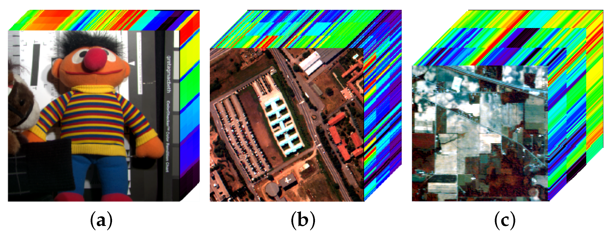
4.2. Experiments on Noiseless HSI Datasets

All methods are evaluated on three HSIs, namely Toy from the CAVE dataset (http://www1.cs.columbia.edu/CAVE/databases/multispectral/), PaviaU and corrected Indian Pines from hyperspectral remote sensing scenes (http://www.ehu.eus/ccwintco/index.php?title=Hyperspectra-Remote-Sensing-Scenes). The Toy is full spectral resolution reflectance data from 400 nm to 700 nm at 10 nm steps (31 bands total), with spatial resolution 512 × 512. The PaviaU dataset contains 103 bands, including 610 × 340 pixels. The Indian Pines is of size 145 × 145 with 10 m spatial resolution and consists of 200 bands via removing 20 noisy bands polluted by water absorption, which covers the wavelength in the range from 400 to 2500 nm by 10 nm spectral resolution. We conducted experiments on the three HSI datasets mainly for the following reasons. (1) The three HSI datasets possess higher spatial-spectral resolutions and richer non-local similarity, which facilitates that the structured sparsity across spatial-spectral domains is employed in our HSI-CSR model. (2) These HSIs are benchmark testing datasets in HSI reconstruction, as presented in [21,22,24,25,40,42,43,45,50,53,54]. (3) We selected the dataset with classification label, Indian Pines, which helps to compare all methods in term of classification accuracy. For the experiment, we cropped a sub-region of 300 × 300 for all bands of Toy and PaviaU, as shown in Figure 3. To validate the performance of proposed method, five different sampling rates (SR), namely 0.02, 0.05, 0.10, 0.15 and 0.20, were considered.

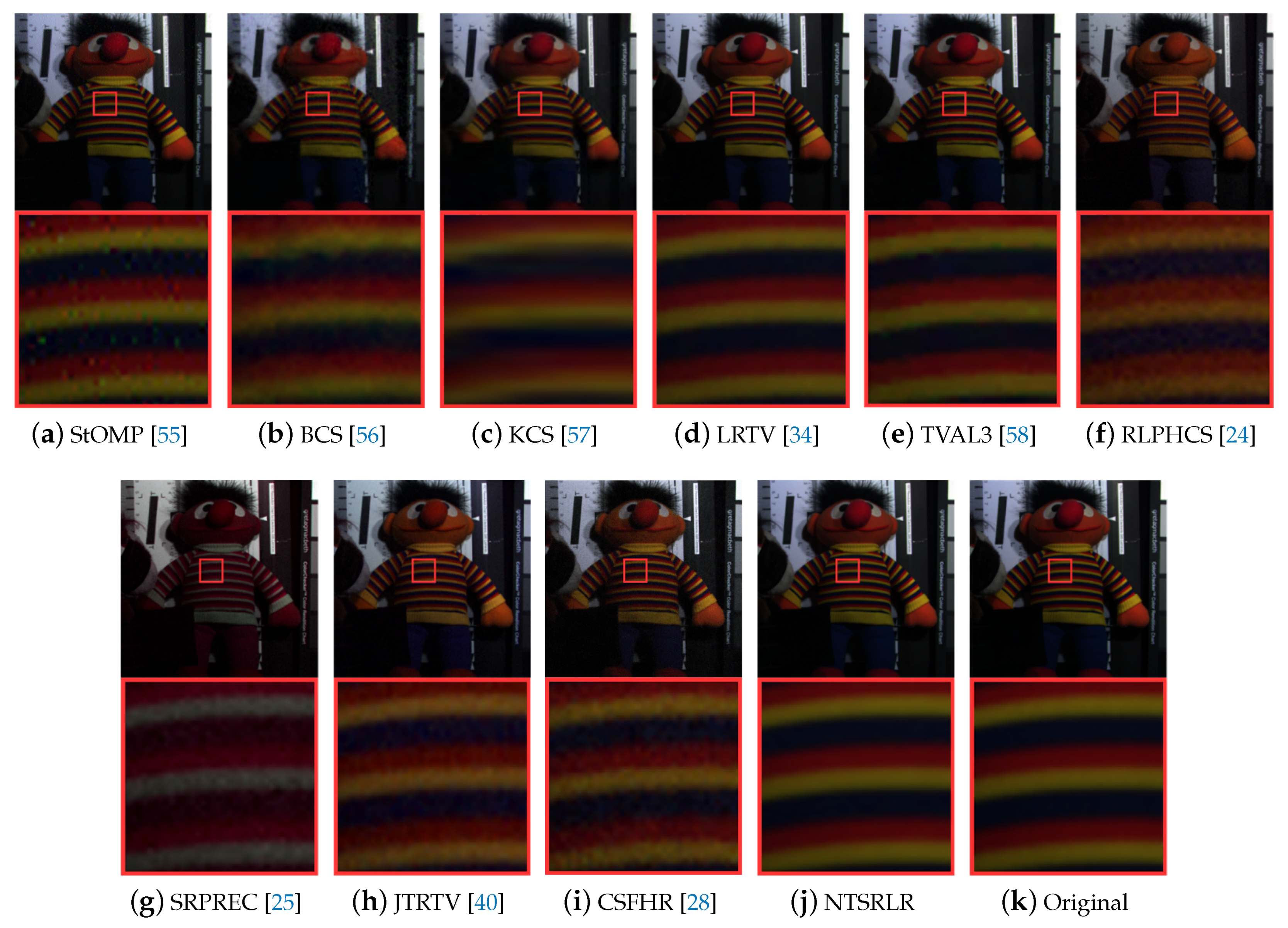
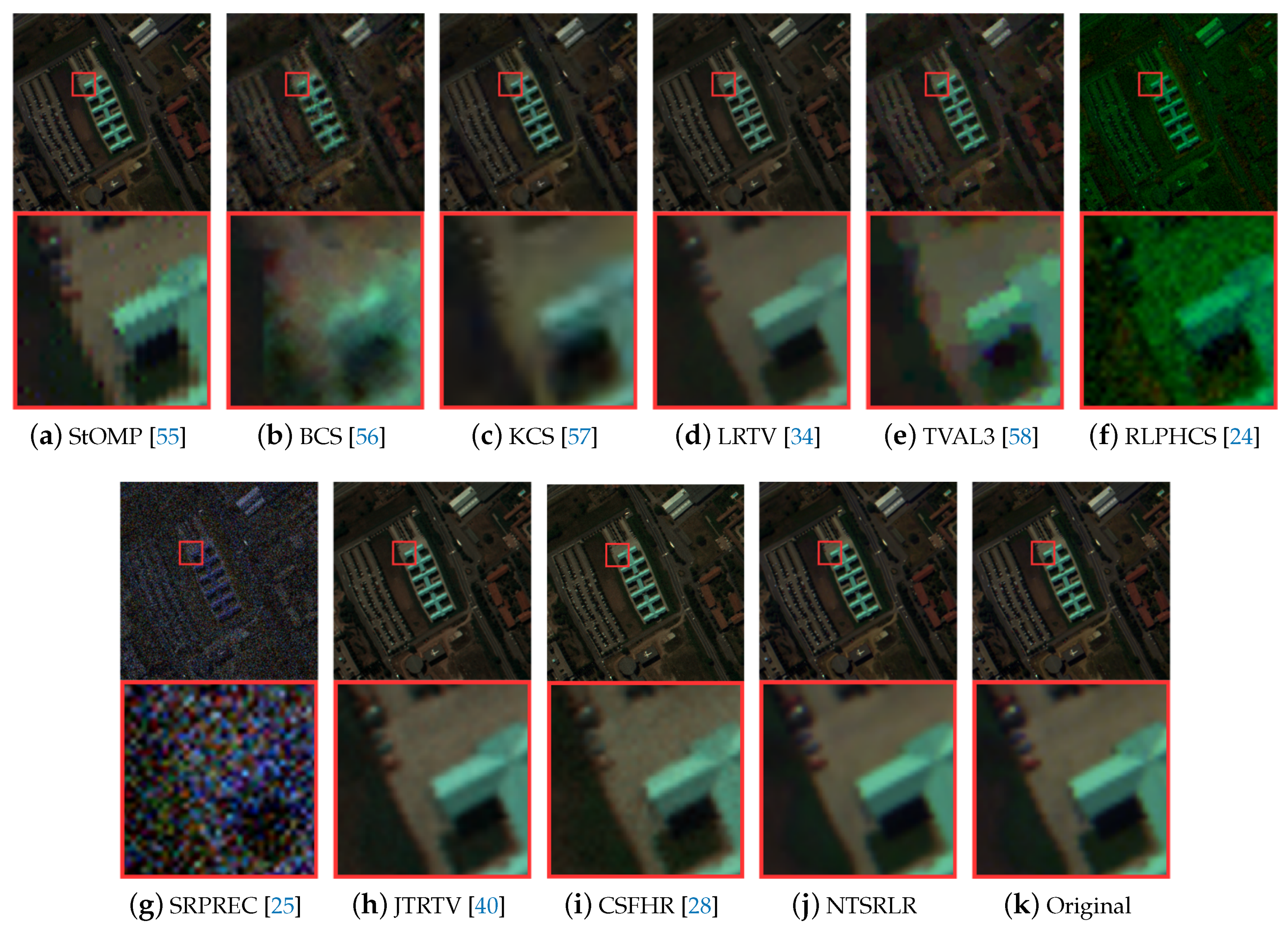
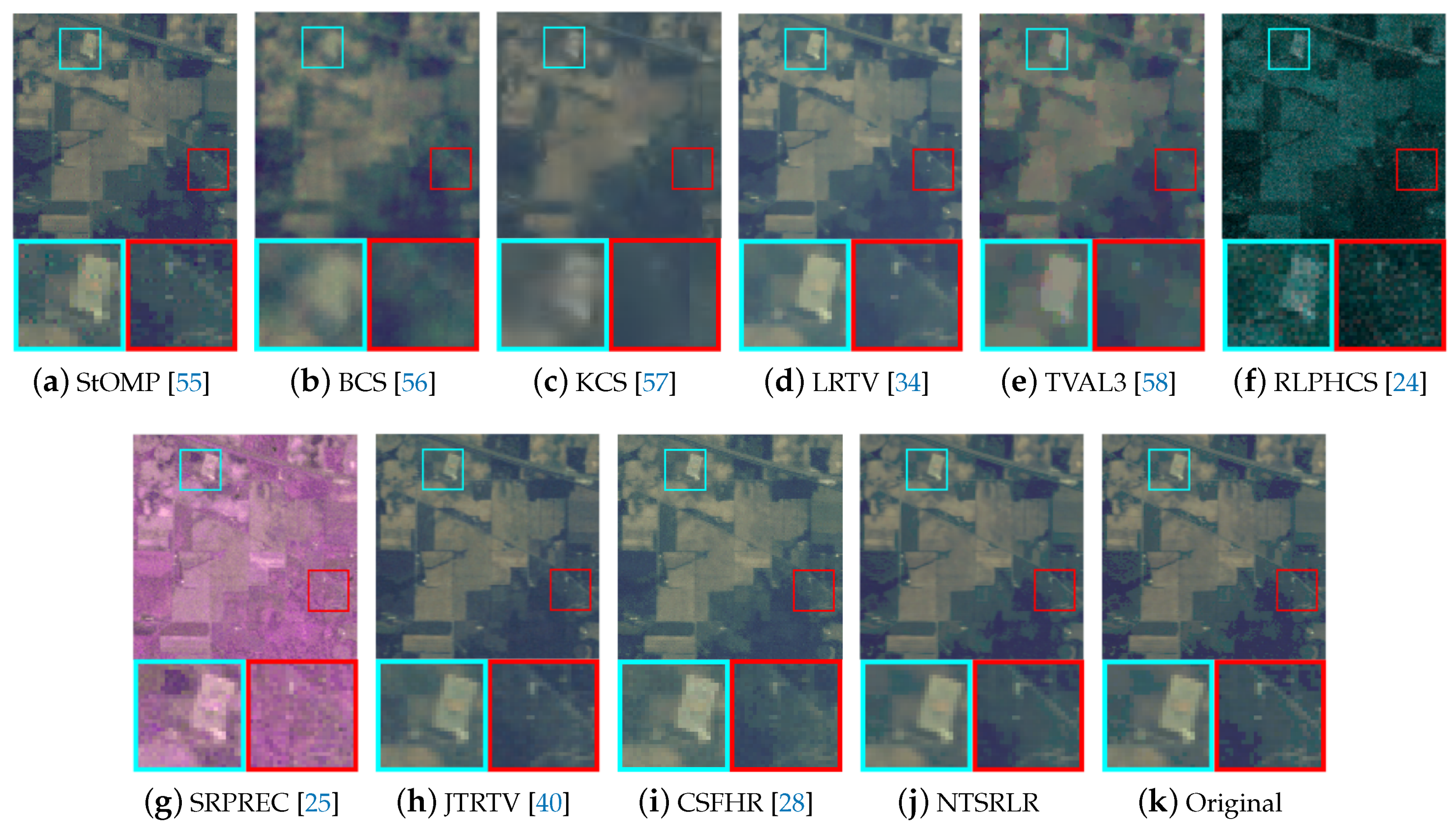
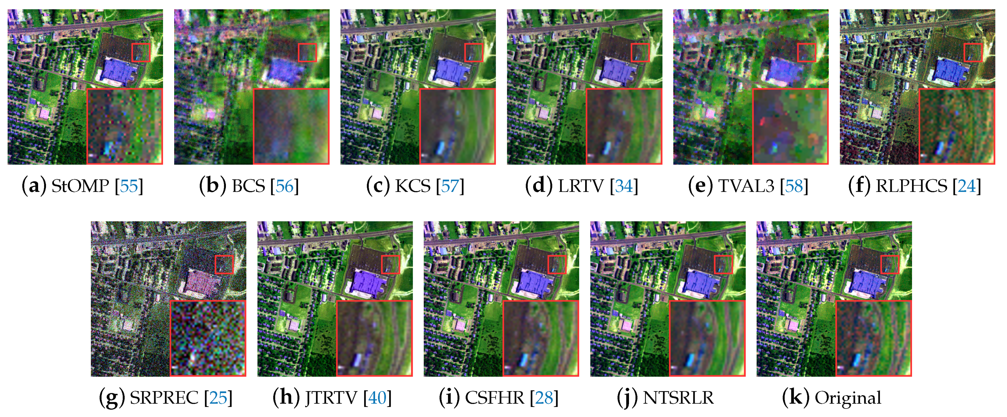
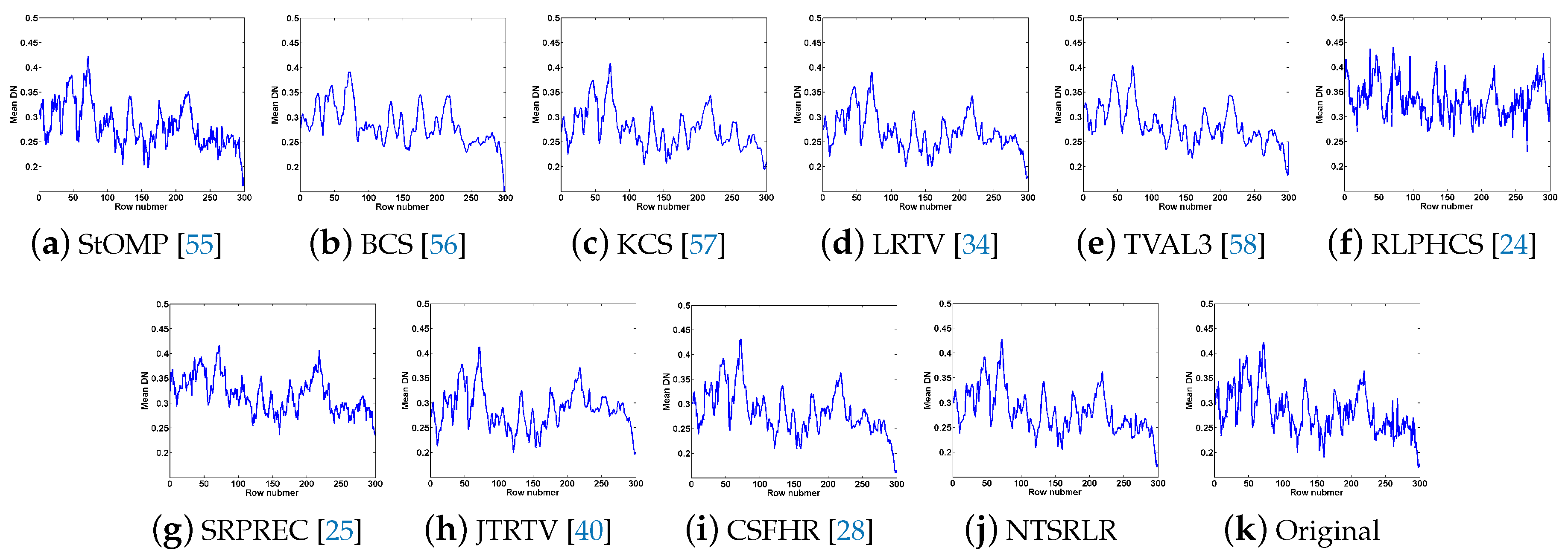
4.2.1. Visual Quality Evaluation

To visually demonstrate the HSI-CSR performances of the proposed method, we present the pseudocolor images with bands (25,15, 5), bands (55, 30, 5), and bands (23, 13, 3) of reconstructed Toy, PaviaU and Indian Pines obtained by all methods under sampling rates of 0.20, 0.10 and 0.15 in Figure 4, Figure 5 and Figure 6, respectively. We have the following observations. (1) All the competing methods achieved relatively good reconstructed results. (2) The proposed method outperformed the other methods, as shown by the enlarged subregion (delineated in a red box), where the large-scale sharp edges and small-scale fine texture features are reconstructed well, as shown in Figure 4, Figure 5 and Figure 6j. (3) The method StOMP produced serious noise during reconstruction and the details are blurred in the results of BCS, KCS and CSFHR. Instead of $l_1$-based sparsity term, the TVAL3 utilizes the TV regularization based on gradient sparsity to preserve the more accurate edges but many details are lost. Although LRTV simultaneously considers the gradient sparsity and low-rankness of the data, the lack of an effective constraint for nonlocal spatial information will generate blurring artifacts. The JTRTV method is a generalization of LRTV for high-dimensional data, although it can deal with the artifacts problem generated by LRTV, it introduces unwanted noises. The RLPHCS and SRPREC consider the structure sparsity based on the reweighted Laplace prior. Nevertheless, their reconstructed results are unsatisfactory and the two methods appear to be virtually powerless for HSI-CSR. We provide following justifications about poor performance of RLPHCS and SRPREC: (1) The two HSI-CSR models use the maximum a posteriori framework to learn the hyperparameters; the accumulation of estimated bias for parameters may lead to a poor HSI-CSR performance. (2) The collected dictionaries in RLPHCS and SRPREC algorithms may not be overcomplete, which do not fully consider the redundant structure over spatial and spectral domain. This demonstrates the effectiveness of NTSRLR technique for HSI-CSR, greatly preserving the local details and structural information of the HSI.

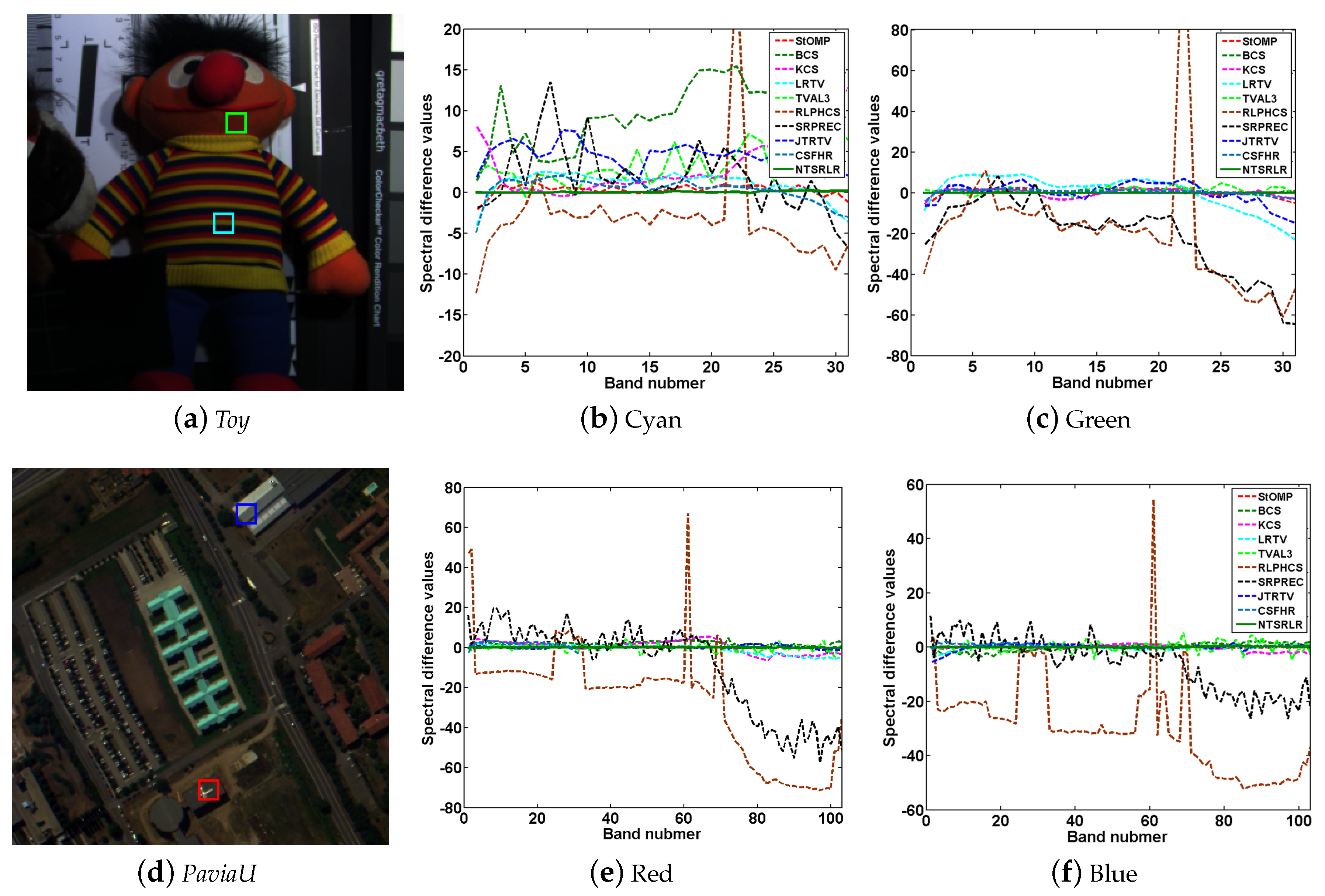
4.2.2. Quantitative Evaluation

In

Table 1. MPSNRs, MSSIMs, and MFSIMs of different CSR methods on three selected HSIs under different sampling rates.

SRs	PQIs	Methods
		StOMP	BCS	KCS	LRTV	TVAL3	RLPHCS	SRPREC	JTRTV	CSFHR	NTSRLR
		[55]	[56]	[57]	[34]	[58]	[24]	[25]	[40]	[28]
Results on Toy
0.02	MPSNR	25.27	18.45	23.39	22.08	22.91	13.19	14.40	17.19	25.87	27.81
	MSSIM	0.7040	0.3499	0.6565	0.6651	0.6364	0.2089	0.2786	0.1601	0.6639	0.7322
	MFSIM	0.8044	0.6937	0.7820	0.8061	0.7397	0.6651	0.6272	0.5033	0.8389	0.8484
0.05	MPSNR	29.35	24.63	26.93	26.51	27.63	13.22	13.89	22.65	29.96	34.22
	MSSIM	0.8256	0.6672	0.7811	0.7873	0.7817	0.2372	0.1929	0.3374	0.7462	0.8930
	MFSIM	0.9189	0.7837	0.8523	0.8783	0.8273	0.6493	0.5480	0.6233	0.8845	0.9423
0.10	MPSNR	29.71	28.24	29.94	32.06	31.81	13.06	15.92	29.93	32.35	40.12
	MSSIM	0.8416	0.8072	0.8641	0.9233	0.8871	0.2034	0.1267	0.6860	0.8418	0.9640
	MFSIM	0.9261	0.8563	0.8987	0.9517	0.9052	0.6163	0.4505	0.8466	0.9255	0.9814
0.15	MPSNR	30.90	29.40	31.88	34.99	33.46	13.69	27.79	31.47	34.99	44.52
	MSSIM	0.8982	0.8429	0.9025	0.9427	0.9141	0.1993	0.7492	0.7673	0.8985	0.9848
	MFSIM	0.9485	0.8777	0.9232	0.9669	0.9282	0.5642	0.9082	0.8894	0.9527	0.9928
0.20	MPSNR	31.75	31.63	33.26	40.54	37.65	13.71	25.74	33.39	38.53	47.86
	MSSIM	0.9345	0.8845	0.9236	0.9808	0.9593	0.2495	0.7384	0.8504	0.9541	0.9925
	MFSIM	0.9617	0.9094	0.9375	0.9876	0.9664	0.6182	0.8942	0.9307	0.9785	0.9965
Results on PaviaU
0.02	MPSNR	28.11	21.74	23.79	23.08	22.99	15.18	14.84	28.04	25.11	29.83
	MSSIM	0.7603	0.4767	0.5486	0.6500	0.5014	0.1562	0.0990	0.6708	0.6923	0.8000
	MFSIM	0.8246	0.6825	0.6743	0.7974	0.6429	0.6808	0.5758	0.8593	0.8095	0.8884
0.05	MPSNR	30.06	24.26	26.59	27.49	25.29	14.38	15.46	35.73	32.74	37.96
	MSSIM	0.8571	0.5572	0.6783	0.8099	0.5914	0.1698	0.1266	0.9235	0.8756	0.9551
	MFSIM	0.9371	0.7379	0.7854	0.8863	0.7132	0.7123	0.6379	0.9666	0.9442	0.9774
0.10	MPSNR	30.40	26.36	29.14	32.99	27.48	15.73	16.00	37.10	34.36	42.15
	MSSIM	0.8223	0.6479	0.7871	0.9158	0.6907	0.1225	0.1157	0.9452	0.9062	0.9794
	MFSIM	0.9409	0.7963	0.8606	0.9479	0.7894	0.5930	0.5461	0.9761	0.9583	0.9905
0.15	MPSNR	31.59	27.08	30.85	33.81	28.33	26.46	28.29	37.39	36.77	44.55
	MSSIM	0.8707	0.6812	0.8422	0.9417	0.7268	0.6771	0.8567	0.9487	0.9417	0.9872
	MFSIM	0.9523	0.8137	0.8981	0.9683	0.8165	0.8738	0.9255	0.9778	0.9741	0.9944
0.20	MPSNR	32.49	28.54	32.13	40.56	30.46	28.14	35.38	38.03	40.56	46.55
	MSSIM	0.9020	0.7445	0.8745	0.9740	0.8057	0.7328	0.9547	0.9548	0.9705	0.9917
	MFSIM	0.9594	0.8518	0.9198	0.9862	0.8745	0.8964	0.9800	0.9807	0.9871	0.9965
Results on Indian Pines
0.02	MPSNR	30.45	33.03	31.46	22.81	30.12	19.51	23.58	30.87	30.85	33.54
	MSSIM	0.7487	0.7692	0.7385	0.4916	0.7839	0.2234	0.4025	0.8010	0.8089	0.8202
	MFSIM	0.8299	0.8128	0.7337	0.8421	0.8026	0.7149	0.8327	0.8102	0.8500	0.8775
0.05	MPSNR	35.70	37.23	33.71	26.77	37.28	16.44	21.01	37.07	36.86	41.15
	MSSIM	0.8693	0.8153	0.7763	0.8057	0.8221	0.0920	0.2944	0.9240	0.8671	0.9470
	MFSIM	0.8639	0.8554	0.7983	0.8936	0.8517	0.4714	0.8125	0.9475	0.9210	0.9553
0.10	MPSNR	40.77	38.97	35.38	34.10	39.66	16.06	25.10	39.29	37.38	44.12
	MSSIM	0.9395	0.8427	0.8165	0.9153	0.8606	0.0614	0.5336	0.9338	0.8798	0.9719
	MFSIM	0.9420	0.8867	0.8491	0.9440	0.8919	0.3846	0.8317	0.9472	0.9439	0.9750
0.15	MPSNR	43.71	39.42	36.39	34.65	40.47	19.62	24.05	39.85	39.27	45.65
	MSSIM	0.9465	0.8478	0.8417	0.9248	0.8743	0.4756	0.4416	0.9354	0.9197	0.9810
	MFSIM	0.9794	0.8942	0.8743	0.9496	0.9056	0.7956	0.7804	0.9476	0.9569	0.9818
0.20	MPSNR	44.92	40.72	37.12	41.66	42.36	20.95	26.07	39.67	41.81	46.96
	MSSIM	0.9350	0.8740	0.8601	0.9670	0.9052	0.5259	0.4957	0.9367	0.9475	0.9863
	MFSIM	0.9772	0.9179	0.8907	0.9748	0.9349	0.8216	0.7966	0.9465	0.9706	0.9858

and

Table 2. SAM and ERGAS comparisons of different CSR methods on three selected HSIs under different sampling rates.

SRs	PQIs	Methods
		StOMP	BCS	KCS	LRTV	TVAL3	RLPHCS	SRPREC	JTRTV	CSFHR	NTSRLR
		[55]	[56]	[57]	[34]	[58]	[24]	[25]	[40]	[28]
Results on Toy
0.02	SAM	0.3040	0.6548	0.3062	0.5096	0.3888	0.9853	0.9707	0.6599	0.4014	0.2810
	ERGAS	165.5	864.5	294.7	362.5	309.7	2411	2740	582.3	178.9	154.8
0.05	SAM	0.2500	0.2781	0.2351	0.3967	0.2886	0.9633	0.9210	0.6532	0.3401	0.2029
	ERGAS	147.8	257.3	193.9	204.3	181.9	2064	2536	321.4	141.5	84.65
0.10	SAM	0.2318	0.1968	0.1894	0.2162	0.2080	0.6234	0.8382	0.4129	0.2750	0.1031
	ERGAS	141.94	170.4	136.9	107.0	113.1	1273	1853	140.3	108.1	35.92
0.15	SAM	0.2629	0.1654	0.1635	0.1940	0.1828	0.4228	0.4562	0.3582	0.2151	0.0998
	ERGAS	123.9	148.6	109.9	78.40	93.82	1262	1620	118.5	79.23	28.08
0.20	SAM	0.1123	0.1471	0.1478	0.1112	0.1294	0.3866	0.4250	0.2964	0.1599	0.0733
	ERGAS	112.5	116.1	94.29	41.20	58.60	978	1305	95.77	53.85	20.86
Results on PaviaU
0.02	SAM	0.1819	0.2223	0.1931	0.1576	0.2460	0.9542	0.9950	0.1722	0.1248	0.1128
	ERGAS	137.8	345.6	264.4	329.0	284.3	2537	3585	156.7	153.8	125.8
0.05	SAM	0.1542	0.1749	0.1512	0.1347	0.2021	0.8849	0.9646	0.0817	0.1019	0.0550
	ERGAS	123.4	245.2	187.6	153.2	213.4	2079	2997	67.56	96.19	50.98
0.10	SAM	0.1447	0.1417	0.121	0.0862	0.1701	0.7069	0.8168	0.0725	0.0905	0.0389
	ERGAS	118.7	188.0	138.7	90.35	165.2	1858	2425	58.58	80.19	32.53
0.15	SAM	0.1116	0.1326	0.1059	0.0708	0.1596	0.2914	0.2368	0.0708	0.0728	0.0315
	ERGAS	103.6	173.3	113.96	77.17	149.8	1247	1921	56.68	61.15	24.90
0.20	SAM	0.0858	0.1178	0.0957	0.0462	0.1359	0.2407	0.0836	0.0674	0.0521	0.0260
	ERGAS	93.40	146.2	98.66	38.73	117.7	1231	1427	52.63	41.26	19.74
Results on Indian Pines
0.02	SAM	0.1511	0.1622	0.1383	0.2774	0.1246	0.9166	0.9476	0.1075	0.1087	0.0821
	ERGAS	143.2	161.8	138.6	759.7	126.5	1723	2297	129.7	198.7	116.0
0.05	SAM	0.1447	0.0830	0.1063	0.0832	0.0911	0.5668	0.8286	0.0553	0.0723	0.0382
	ERGAS	89.48	88.69	119.2	233.2	87.85	1558	1988	64.84	152.6	49.62
0.10	SAM	0.0434	0.0728	0.0888	0.0587	0.0743	0.4821	0.6523	0.0515	0.0659	0.0282
	ERGAS	38.77	74.77	96.91	43.08	68.53	1078	1323	58.37	127.4	35.96
0.15	SAM	0.0365	0.0714	0.0799	0.0498	0.0693	0.3914	0.4663	0.0505	0.0549	0.0229
	ERGAS	34.98	72.32	86.24	37.45	62.99	917	1258	56.15	78.07	30.81
0.20	SAM	0.0295	0.0622	0.0741	0.0344	0.0586	0.2749	0.4590	0.0481	0.0553	0.0190
	ERGAS	31.39	61.87	79.43	33.59	51.61	366	982	50.78	59.69	27.19

, we provide the performance of all methods using MPSNR, MSSIM, MFSIM, SAM and ERGAS results, over all the spectral bands in Toy, PaviaU and Indian Pines. We highlight the best results for each case in bold in the current and following tables. The proposed method outperforms the other approaches under all sampling rates and in particular the PQIs are better than the recent JTRTV. At sampling rate $\rho$ = 0.02, NTSRLR improves the MPSNR at least 10 dB more than JTRTV on the Toy, 1.3 dB better on the PaviaU, and 2.7 dB better on the Indian Pines. For $\rho$ = 0.20, the average gain of MPSNR values of NTSRLR are more amplified compared with JTRTV, up to 14 dB on Toy, 8 dB on PaviaU and 7 dB on Indian Pines. MSSIM, MFSIM, SAM and ERGAS values values under three HSI datasets further confirm the robustness of the proposed method at all sampling rates. Although LRTV is second best method, obviously it still is inferior to ours by visual quality evaluation. Since NTSRTR explores the underlying nonlocal structure of an HSI by the tensor sparse representation and low-rank modeling, it gives higher MPNSR, MSSIM, and MFSIM values, and smaller SAM and ERGAS than the other methods, which only consider the local or single sparsity prior.

The values of PSNR, SSIM and FSIM across all bands on Indian Pines under sampling rate $\rho$ = 0.10 are presented in Figure 7. The proposed method achieves the best PSNR, SSIM and FSIM values in most bands of the HSI, which also further validates the robustness of the proposed method over all spectral bands. To further illustrate the superiority of proposed NTSRLR on spectrum reconstruction, we chose four regions in Toy and PaviaU datasets shown Figure 8a,d; the average reflectance differences were calculated between reconstructed spectra and original spectra across all bands. The curves of those average reflectance differences are plotted in Figure 8b,c for Toy and Figure 8e,f for PaviaU. It is obvious that the reflectance difference between the reference and the reconstruction by NTSRLR is close to zero—much better than the other comparison methods.

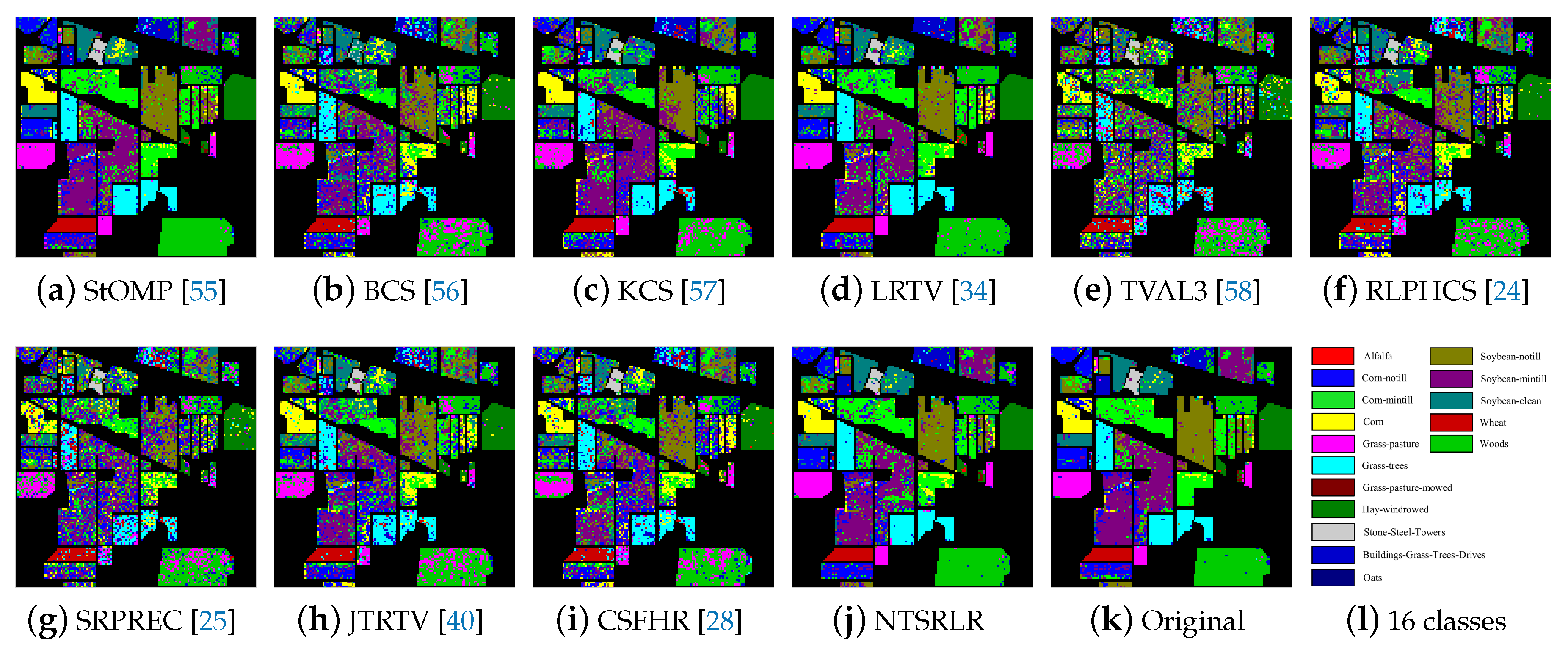
4.2.3. Classification Performance on Indian Pines Dataset

The classification accuracy of the HSI with different algorithms was employed to further verify the effectiveness of the proposed method. Under the same circumstance, we chose the support vector machine (SVM) [63] and overall accuracy (OA) as the classifier and evaluation index, respectively. During the classification results with SVM algorithm, we used 16 ground-truth classes in Indian Pines and 10% randomly generated training sets from each class to test the classification accuracy. The classification results with different HSI-CSR methods under sampling rate $\rho$ = 0.20 are revealed in Figure 9a–j. The OA are given in

Table 3. Classification performance comparison before and after CSR on Indian Pines under different sampling rates.

SRs	StOMP	BCS	KCS	LRTV	TVAL3	RLPHCS	SRPREC	JTRTV	CSFHR	NTSRLR	Original
	[55]	[56]	[57]	[34]	[58]	[24]	[25]	[40]	[28]
0.02	71.19%	50.64%	52.37%	60.96%	51.85%	29.61%	10.51%	20.03%	53.21%	73.69%	86.37%
0.05	75.70%	57.83%	56.18%	69.64%	57.83%	36.66%	13.32%	54.47%	59.17%	77.32%
0.10	76.32%	59.01%	62.01%	71.24%	60.92%	41.82%	14.62%	55.66%	62.98%	79.31%
0.15	78.41%	63.80%	65.80%	77.03%	62.70%	45.53%	45.53%	56.84%	65.24%	80.26%
0.20	80.28%	68.73%	70.73%	79.19%	65.73%	46.57%	57.83%	58.13%	67.70%	81.79%

. As shown in Figure 9j, the classification results in original HSI appear continuous, and the OA is 86.37%. As shown in Figure 9i, the classification results of NTSRLR still show a continuous phenomenon, and the OA of NTSRLR is closer to the reference value. However, the classification results of other methods are more fragmentary in most regions of the image, with lower OA values.

4.3. Robustness for Noise Suppression during HSI-CSR

To further evaluate the effectiveness and robustness of proposed HSI-CSR method for noise suppression, we chose the Urban dataset (http://www.tec.army.mil/hypercube) contaminated by different degrees of mixture noise, which was with size of 307 × 307 and 4 m spatial resolution, and covers the wavelength in the range from 400 to 2400 nm by 10 nm spectral resolution. Under same competing methods, we removed 24 bands seriously affected by atmospheric attenuations and water absorptions, and finally reserved 186 bands for the dataset.

We present the pseudocolor image with bands (186, 131, 1), in which the input data is polluted by Gaussian noise and stripes, as shown in Figure 10k. The CSR results produced by StOMP, BCS, CSFHR and TVAL3 could neither recover the original HSI nor perform the denoising task well. Instead, the methods RLPHCS and SRPREC amplified the noise. Although the methods KCS, LRTV and JTRTV could suppress the noise to some extent, they lost the edges and textural details when compared to NTSRLR.

Furthermore, we present the quantitative comparisons by showing the horizontal mean profiles of bands 1 and 186 in Urban dataset before and after CSR in Figure 11 and Figure 12. The horizontal axis in the figure denotes the row number, and the vertical axis represents the mean gray value of each row. As shown in Figure 11k and Figure 12k, the profiles have huge fluctuation due to the disturbance of noises. After CSR, the fluctuation has been moderately alleviated. Evidently, the profiles with the proposed NTSRLR method are more natural and smoother. The over-smooth profiles corresponding to BCS are mainly due to the image blurring. This further substantiates the efficiency and robustness of the proposed HSI-CSR method for noise suppression.

Here, we give the theoretical analysis to explain why the proposed HSI-CSR algorithm is able to suppress noise at the same time. The primary cause is that proposed NTSRLR contributes the noise suppression to the joint tensor sparse and low-rank constraint on nonlocal cubes. The work in [64] refers to the fact that the low-rank representation for those nonlocal similar patches to a given patch offer helpful remedy for its better image denoising. For tensor data, one can obtain the same results when unfolding a tensor into a matrix along certain mode, and the nonlocal tensor low-rank term of NTSRLR model can simultaneously provide complementary low-rank structures along all modes to promote the denoising performance of tensor data. Therefore, the noise of HSI can be suppressed to some extent. Besides, the research is [53,54] has demonstrated the effectiveness of tensor sparse models in multi-dimensional signals denoising, which verifies the positive impact of NTSRLR on noise suppression from the perspective of tensor sparse representation.

Note that we removed all noisy bands and preserved only 171 bands for quantitative assessment.

Table 4. MPSNRs, MSSIMs, MFSIMs ERGAS and SAM of different CSR methods on Urban with different sampling rates.

SRs	PQIs	Methods
		StOMP	BCS	KCS	LRTV	TVAL3	RLPHCS	SRPREC	JTRTV	CSFHR	NTSRLR
		[55]	[56]	[57]	[34]	[58]	[24]	[25]	[40]	[28]
0.10	MPSNR	19.63	16.95	23.63	24.76	17.79	22.04	15.13	27.74	26.76	30.88
	MSSIM	0.6523	0.4147	0.8152	0.8705	0.4423	0.8155	0.4245	0.8959	0.8933	0.9471
	MFSIM	0.8841	0.6918	0.8916	0.9277	0.6562	0.9088	0.7711	0.9561	0.9279	0.9746
	ERGAS	280.2	380.4	184.2	159.6	346.3	261.6	480.9	111.5	109.8	76.89
	SAM	0.2884	0.2157	0.1551	0.1197	0.2644	0.2737	0.4775	0.1196	0.1252	0.0682
0.15	MPSNR	20.61	17.45	25.78	26.40	18.48	24.16	20.94	27.94	28.27	33.51
	MSSIM	0.7088	0.4546	0.8740	0.9134	0.4924	0.8442	0.8306	0.8992	0.9064	0.9662
	MFSIM	0.8972	0.7138	0.9242	0.9575	0.6946	0.9284	0.9016	0.9580	0.9582	0.9845
	ERGAS	250.4	359.7	145.4	122.9	320.0	202.4	296.3	108.9	91.23	56.89
	SAM	0.2461	0.2076	0.1310	0.1024	0.2518	0.2202	0.2885	0.1180	0.1075	0.0564
0.20	MPSNR	20.93	18.72	27.37	33.26	20.35	25.99	25.24	28.40	30.11	35.62
	MSSIM	0.7274	0.5509	0.9051	0.9664	0.6133	0.8583	0.9034	0.9040	0.9275	0.9762
	MFSIM	0.9011	0.7645	0.9418	0.9840	0.7810	0.9459	0.9445	0.9608	0.9705	0.9896
	ERGAS	241.4	310.8	122.3	59.45	259.0	165.8	183.7	103.1	67.60	44.66
	SAM	0.2323	0.1879	0.1156	0.0592	0.2207	0.1831	0.1859	0.1149	0.0828	0.0481

presents MPSNR, MSSIM, MFSIM ERGAS and SAM of all methods under sampling rates 0.10, 0.15 and 0.20. It can be seen that our method not only recovered the structural and perceptual feature of Urban dataset, but also preserved better spectral information.

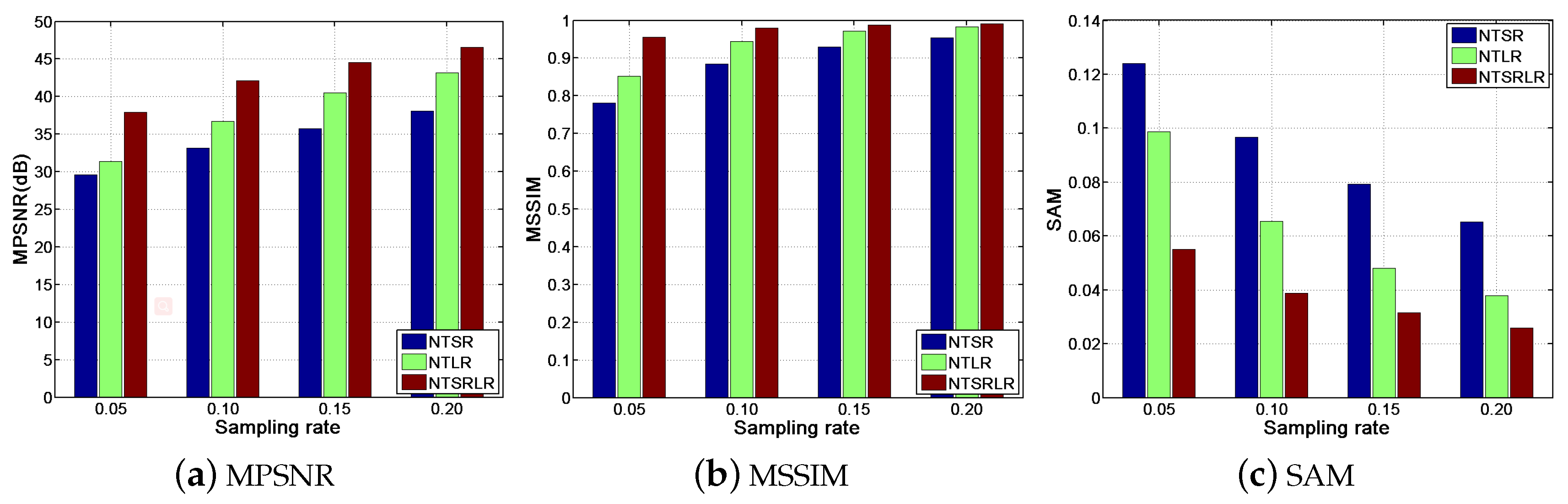
4.4. Effectiveness Analysis of Single NTSR or NTLR Constraint

To further demonstrate the effectiveness of nonlocal tensor sparse representation and low-rank regularization in our model, we conducted two more experiments using the PaviaU dataset. The first experiment was to perform CSR without the nonlocal tensor low-rank regularization term, and the reconstructed HSI was achieved solely by nonlocal tensor sparse representation (NTSR). The second experiment was a reconstruction with the nonlocal tensor low-rank regularization method, but without NTSR, which is abbreviated as NTLR.

Figure 13 shows the comparison results of MPSNR, MSSIM and SAM of all methods under sampling rates from 0.05 to 0.20 with interval 0.05. Compared with other methods, the proposed NTSRLR obtained larger MPSNRs and MSSIMs, and smaller errors as measured by SAM under different sampling rates. In particular, when the sampling rate is small, the results from NTSRLR are significantly better than the NTSR and NTLR, which are based on a single constraint. This provides additional evidence for the effectiveness of the proposed method from the perspective of having integrated constraints with both non-local sparse representation and low rankness in our model.

4.5. Computational Complexity Analysis

For an input HSI $\mathcal{X}\in {\mathbb{R}}^{W\times H\times S}$, the number of FBCs is $P=O\left(WH\right)$, the size of each FBC group is $wh\times s\times S$, where s is number of FBCs in each group. The computation cost seems not very small for quite large P. However, CSR on the P FBCs can be processed in parallel, each with relatively small computational complexity. The computational complexity of the proposed algorithm that mainly lies in the update of ${\mathcal{M}}_{p\left(i\right)},{\mathrm{U}}_{ip}(i=1,2,3)$. Updating ${\mathrm{U}}_{ip}$ requires computing an SVD of $I_i\times I_i$ matrix, and updating ${\mathcal{M}}_{p\left(i\right)}$ requires computing an SVD of $I_i\times ({\prod }_{j\ne i}{I}_j)$ matrix. Relatively, the other variables ${\mathcal{G}}_p,x$ and multipliers updating will not consume lots of running time.

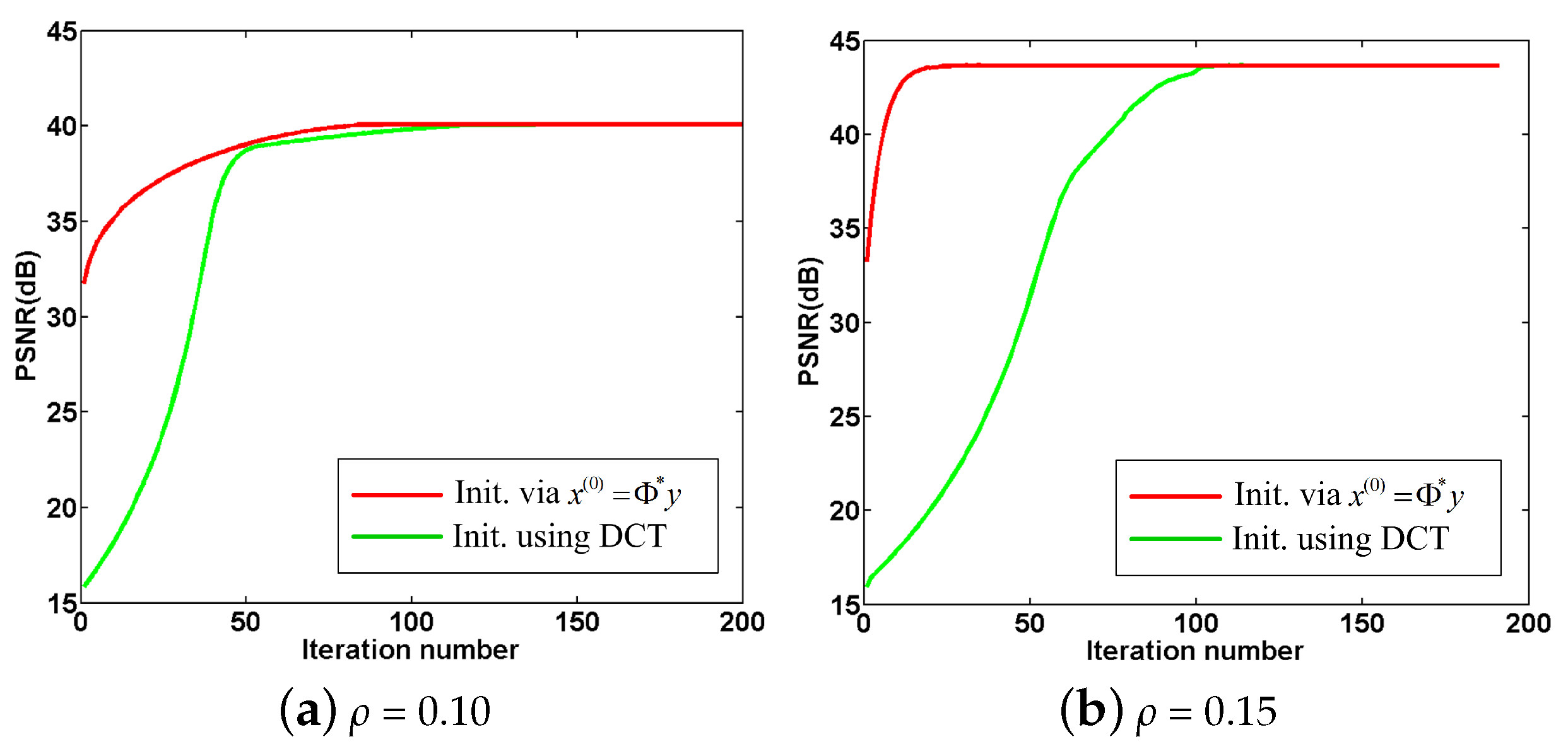
4.6. Convergence Analysis

Lastly, we have conducted experiments to show the convergence of our method using the Toy and Indian Pines dataset as examples under different sampling rates and different initializations. Figure 14 plots the PSNRs versus iteration numbers for the tested HSIs when the sampling rates are at 0.10 for Toy and 0.15 for Indian Pines, when using initialization $x={\Phi }^{*}y$ and DCT. As can be seen, the different initialization ways can provide quite close solutions, which indicates the performance of proposed algorithm is not sensitive to initialization. However, the two initialization ways possess different rates of convergence, and, by contrast, the initialization via DCT requires only a small number of iterations to get to the final PSNR. Therefore, we adopted the initialization strategy based on DCT to speed up our algorithm. Besides, the value of PSNR will become a constant when the algorithm converges. Thus, in the experiment, we set the maximum number of iterations for termination condition.

4.7. Parameters Analysis

There are four parameters ${\left\{{\lambda }_i\right\}}_{i=1}^4$ in the proposed model. Considering the different roles of nonlocal tensor sparseness and low-rankness terms, we conducted two more experiments on PaviaU dataset in Section 4.4. The results of MPSNR, MSSIM and SAM demonstrate the nonlocal tensor low-rank regularization term plays a more important role in proposed model than nonlocal tensor sparse representation term. It implies that the nonlocal tensor low-rankness term should be assigned a greater weight to balance the two parts. Therefore, we set ${\lambda }_2=1$ and ${\lambda }_3=10$ in all our experiments. Correspondingly, we can regard the other two parts with ${\lambda }_{\mathbf{1}}$ and ${\lambda }_4$ tradeoff as loyalty terms of the nonlocal tensor sparseness and low-rankness; it is reasonable to obtain a greater value for ${\lambda }_4$, and we set ${\lambda }_1=0.02$ and ${\lambda }_4=250$, as suggested in [42].

Besides, the spatial size of cube and the number of non-local similar cubes are two key parameters. Some research [17,18,30,41] reports that the spatial size of cube and the number of non-local similar cubes are dependent on sampling rates. The higher the sampling rate is, the more detailed information of texture and structure the HSI loses. For this reason, the bigger spatial size and more non-local similar cubes are beneficial to provide extra knowledge to further promote the HSI reconstruction performance. Thus, according to the parameter setting principle in [17,18,30,41], we set spatial size to 6 × 6, 7 × 7, 8 × 8, 9 × 9 and 10 × 10 for $\rho$ = 0.20, 0.15, 0.10, 0.05 and 0.02, respectively; and the corresponding number of non-local similar cubes are set to 50, 55, 60, 65 and 70.

5. Conclusions

In this paper, we propose a novel method for hyperspectral image compressed sensing reconstruction by non-local tensor sparse representation and low-rank regularization. The proposed method considers intrinsic structured sparsity, where the nonlocal similarity between spatial cubes and the global correlation across all bands are considered fully. Each cube group contains similar structures; its tensor-based sparsity and low-rank properties can be regarded as very valuable priors. Experimental results reveal that the proposed methods outperform the state-of-the-art methods in term of visual inspection, quantitative and classification accuracy assessment. The proposed method is also superior in noise suppression. We also conclude that it is advantageous to have integrated constraints using both non-local tensor sparse representation and low-rankness rather than using only one of them in our model.

References

1. Yang, J.; Zhao, Y.; Chan, J.C.-W. Learning and transferring deep joint spectral—Spatial features for hyperspectral classification. IEEE Trans. Geosci. Remote Sens. 2017, 55, 4729–4742. [Google Scholar] [CrossRef]
2. Yuan, Y.; Lin, J.; Wang, Q. Hyperspectral image classification via multitask joint sparse representation and stepwise MRF optimization. IEEE Trans. Cybern. 2016, 46, 2966–2977. [Google Scholar] [CrossRef]
3. Liu, Y.; Shi, Z.; Zhang, G.; Chen, Y.; Li, S.; Hong, Y.; Shi, T.; Wang, J.; Liu, Y. Application of Spectrally Derived Soil Type as Ancillary Data to Improve the Estimation of Soil Organic Carbon by Using the Chinese Soil Vis-NIR Spectral Library. Remote Sens. 2018, 10, 1747. [Google Scholar] [CrossRef]
4. Khelifi, F.; Bouridane, A.; Kurugollu, F. Joined spectral trees for scalable spiht-based multispectral image compression. IEEE Trans. Multimed. 2008, 10, 316–329. [Google Scholar] [CrossRef]
5. Christophe, E.; Mailhes, C.; Duhamel, P. Hyperspectral image compression: Adapting spiht and ezw to anisotropic 3-d wavelet coding. IEEE Trans. Image Process. 2008, 17, 2334–2346. [Google Scholar] [CrossRef] [PubMed]
6. Töreyın, B.U.; Yilmaz, O.; Mert, Y.M.; Türk, F. Lossless hyperspectral image compression using wavelet transform based spectral decorrelation. In Proceedings of the IEEE 7th International Conference on Recent Advances in Space Technologies (RAST), Istanbul, Turkey, 16–19 June 2015; pp. 251–254. [Google Scholar]
7. Wang, L.; Wu, J.; Jiao, L.; Shi, G. Lossy-to-lossless hyperspectral image compression based on multiplierless reversible integer TDLT/KLT. IEEE Geosci. Remote Sens. Lett. 2009, 6, 587–591. [Google Scholar] [CrossRef]
8. Mielikainen, J.; Toivanen, P. Clustered DPCM for the lossless compression of hyperspectral images. IEEE Trans. Geosci. Remote Sens. 2003, 41, 2943–2946. [Google Scholar] [CrossRef]
9. Du, Q.; Fowler, J.E. Hyperspectral image compression using JPEG2000 and principal component analysis. IEEE Geosci. Remote Sens. Lett. 2007, 4, 201–205. [Google Scholar] [CrossRef]
10. Du, Q.; Ly, N.; Fowler, J.E. An operational approach to PCA+JPEG2000 compression of hyperspectral imagery. IEEE J. Sel. Top. Appl. Earth Observ. Remote Sens. 2014, 7, 2237–2245. [Google Scholar] [CrossRef]
11. Donoho, D.L. Compressed sensing. IEEE Trans. Inf. Theory 2006, 52, 1289–1306. [Google Scholar] [CrossRef]
12. Boufounos, D.; Liu, D.; Boufounos, P.T. A lecture on compressive sensing. IEEE Signal Process. Mag. 2007, 24, 1–9. [Google Scholar]
13. Huang, J.; Zhang, T.; Metaxas, D. Learning with structured sparsity. J. Mach. Learn. Res. 2011, 12, 3371–3412. [Google Scholar]
14. Tan, M.; Tsang, I.W.; Wang, L. Matching pursuit LASSO part I: Sparse recovery over big dictionary. IEEE Trans. Signal Process. 2015, 63, 727–741. [Google Scholar] [CrossRef]
15. Candes, E.J.; Wakin, M.B.; Boyd, S.P. Enhancing sparsity by reweighted l1 minimization. J. Fourier Anal. Appl. 2008, 14, 877–905. [Google Scholar] [CrossRef]
16. Chartrand, R.; Yin, W. Iterative Reweighted Algorithms for Compressive Sensing. In Proceedings of the IEEE International Conference on Acoust. Speech Signal Process, Las Vegas, NV, USA, 31 March–4 April 2008; pp. 3869–3872. [Google Scholar]
17. Dong, W.; Wu, X.; Shi, G. Sparsity fine tuning in wavelet domain with application to compressive image reconstruction. IEEE Trans. Image Process. 2014, 23, 5249–5262. [Google Scholar] [CrossRef]
18. Dong, W.; Shi, G.; Li, X.; Ma, Y.; Huang, F. Compressive sensing via nonlocal low-rank regularization. IEEE Trans. Image Process. 2014, 23, 3618–3632. [Google Scholar] [CrossRef] [PubMed]
19. Dong, W.; Li, X.; Zhang, L.; Shi, G. Sparsity-based image denoising via dictionary learning and structural clustering. In Proceedings of the Computer Vision and Pattern Recognition (CVPR), Colorado Springs, CO, USA, 20–25 June 2011; pp. 457–464. [Google Scholar]
20. Mairal, J.; Bach, F.; Ponce, J.; Sapiro, G.; Zisserman, A. Non-local sparse models for image restoration. In Proceedings of the IEEE 12th International Conference on Computer Vision, Kyoto, Japan, 29 September–2 October 2009; pp. 2272–2279. [Google Scholar]
21. Zhang, L.; Wei, W.; Zhang, Y.; Yan, H.; Li, F.; Tian, C. Locally similar sparsity-based hyperspectral compressive sensing using unmixing. IEEE Trans. Comput. Imaging 2016, 2, 86–100. [Google Scholar] [CrossRef]
22. Wang, L.; Feng, Y.; Gao, Y.; Wang, Z.; He, M. Compressed sensing reconstruction of hyperspectral images based on spectral unmixing. IEEE J. Sel. Topics Appl. Earth Observ. Remote Sens. 2018, 11, 1266–1284. [Google Scholar] [CrossRef]
23. Li, C.; Sun, T.; Kelly, K.F.; Zhang, Y. A compressive sensing and unmixing scheme for hyperspectral data processing. IEEE Trans. Image Process. 2012, 21, 1200–1210. [Google Scholar]
24. Zhang, L.; Wei, W.; Tian, C.; Li, F.; Zhang, Y. Exploring structured sparsity by a reweighted laplace prior for hyperspectral compressive sensing. IEEE Trans. Image Process. 2016, 25, 4974–4988. [Google Scholar] [CrossRef]
25. Zhang, L.; Wei, W.; Zhang, Y.; Shen, C.; Hengel, A.V.D.; Shi, Q. Dictionary learning for promoting structured sparsity in hyperspectral compressive sensing. IEEE Trans. Geosci. Remote Sens. 2016, 54, 7223–7235. [Google Scholar] [CrossRef]
26. Fu, W.; Li, S.; Fang, L.; Benediktsson, J.A. Adaptive spectral—Spatial compression of hyperspectral image with sparse representation. IEEE Trans. Geosc. Remote Sens. 2017, 55, 671–682. [Google Scholar] [CrossRef]
27. Lin, X.; Liu, Y.; Wu, J.; Dai, Q. Spatial-spectral encoded compressive hyperspectral imaging. ACM Trans. Graphics (TOG) 2014, 33, 233. [Google Scholar] [CrossRef]
28. Zhang, L.; Wei, W.; Zhang, Y.; Shen, C.; Hengel, A.V.D.; Shi, Q. Cluster sparsity field: An internal hyperspectral imagery prior for reconstruction. Int. J. Comput. Vis. 2015, 11, 1–25. [Google Scholar] [CrossRef]
29. Meza, P.; Ortiz, I.; Vera, E.; Martinez, J. Compressive hyperspectral imaging recovery by spatial-spectral non-local means regularization. Opt. Express 2018, 26, 7043–7055. [Google Scholar] [CrossRef] [PubMed]
30. Wei, J.; Huang, Y.; Lu, K.; Wang, L. Nonlocal low-rank-based compressed sensing for remote sensing image reconstruction. IEEE Geosci. Remote Sens. Lett. 2016, 13, 1557–1561. [Google Scholar] [CrossRef]
31. Khan, Z.; Shafait, F.; Mian, A. Joint group sparse pca for compressed hyperspectral imaging. IEEE Trans. Image Process. 2015, 24, 4934–4942. [Google Scholar] [CrossRef] [PubMed]
32. Eason, D.T.; Andrews, M. Total variation regularization via continuation to recover compressed hyperspectral images. IEEE Trans. Image Process. 2015, 24, 284–293. [Google Scholar] [CrossRef] [PubMed]
33. Jia, Y.; Luo, Z. Weighted total variation iterative reconstruction for hyperspectral pushbroom compressive imaging. J. Image Process. Theory Appl. 2016, 1, 6–10. [Google Scholar]
34. Golbabaee, M.; Vandergheynst, P. Joint trace/TV norm minimization: A new efficient approach for spectral compressive imaging. In Proceedings of the 19th IEEE International Conference on Image Processing (ICIP), Orlando, FL, USA, 30 September–3 October 2012; pp. 933–936. [Google Scholar]
35. Karami, A.; Yazdi, M.; Mercier, G. Compression of hyperspectral images using discerete wavelet transform and Tucker decomposition. IEEE J. Sel. Top. Appl. Earth Observ. Remote Sens. 2012, 5, 444–450. [Google Scholar] [CrossRef]
36. Wang, L.; Bai, J.; Wu, J.; Jeon, G. Hyperspectral image compression based on lapped transform and Tucker decomposition. Signal Process. Image Commun. 2015, 36, 63–69. [Google Scholar] [CrossRef]
37. Zhang, L.; Zhang, L.; Tao, D.; Huang, X.; Du, B. Compression of hyperspectral remote sensing images by tensor approach. Neurocomputing 2015, 147, 358–363. [Google Scholar] [CrossRef]
38. Fang, L.; He, N.; Lin, H. CP tensor-based compression of hyperspectral images. J. Opt. Image Sci. Vis. 2017, 34, 252. [Google Scholar] [CrossRef] [PubMed]
39. Yang, S.; Wang, M.; Li, P.; Jin, L.; Wu, B.; Jiao, L. Compressive hyperspectral imaging via sparse tensor and nonlinear compressed sensing. IEEE Trans. Geosci. Remote Sens. 2015, 53, 5943–5957. [Google Scholar] [CrossRef]
40. Wang, Y.; Lin, L.; Zhao, Q.; Yue, T.; Meng, D.; Leung, Y. Compressive sensing of hyperspectral images via joint tensor tucker decomposition and weighted total variation regularization. IEEE Geosci. Remote Sens. Lett. 2017, 14, 2457–2461. [Google Scholar] [CrossRef]
41. Du, B.; Zhang, M.; Zhang, L.; Hu, R.; Tao, D. PLTD: Patch-based low-rank tensor decomposition for hyperspectral images. IEEE Trans. Multimed. 2016, 19, 67–79. [Google Scholar] [CrossRef]
42. Xie, Q.; Zhao, Q.; Meng, D.; Xu, Z.; Gu, S.; Zuo, W.; Zhang, L. Multispectral images denoising by intrinsic tensor sparsity regularization. In Proceedings of the IEEE Conference on Computer Vision and Pattern Recognition, Las Vegas, NV, USA, 27–30 June 2016; pp. 1692–1700. [Google Scholar]
43. Peng, Y.; Meng, D.; Xu, Z.; Gao, C.; Yang, Y.; Zhang, B. Decomposable nonlocal tensor dictionary learning for multispectral image denoising. In Proceedings of the IEEE Conference on Computer Vision and Pattern Recognition, Columbus, OH, USA, 23–28 June 2014; pp. 2949–2956. [Google Scholar]
44. Boyd, S.; Parikh, N.; Chu, E.; Peleato, B.; Eckstein, J. Distributed optimization and statistical learning via the alternating direction method of multipliers. Found. Trends Mach. Learn. 2011, 3, 1–122. [Google Scholar] [CrossRef]
45. Xue, J.; Zhao, Y.; Hao, J. Tensor non-local low-rank regularization for recovering compressed hyperspectral images. In Proceedings of the IEEE International Conference on Image Processing (ICIP), Beijing, China, 17–20 September 2017; pp. 3046–3050. [Google Scholar]
46. Kolda, T.G.; Bader, B.W. Tensor decompositions and applications. SIAM Rev. 2009, 51, 455–500. [Google Scholar] [CrossRef]
47. Schwab, H. For most large underdetermined systems of linear equations the minimal l1 solution is also the sparsest solution. Commun. Pur Appl. Math. 2006, 59, 797–829. [Google Scholar]
48. Daubechies, I.; Defrise, M.; Mol, C.D. An iterative thresholding algorithm for linear inverse problems with a sparsity constraint. Commun. Pure Appl. Math. 2004, 57, 1413–1457. [Google Scholar] [CrossRef] [Green Version]
49. Zhang, X.; Burger, M.; Bresson, X.; Osher, S. Bregmanized nonlocal regularization for deconvolution and sparse reconstruction. SIAM J. Imag. Sci. 2010, 3, 253–276. [Google Scholar] [CrossRef]
50. Xue, J.; Zhao, Y.; Liao, W.; Kong, S.G. Joint spatial and spectral low-rank regularization for hyperspectral image denoising. IEEE Trans. Geosci. Remote Sens. 2018, 56, 1940–1958. [Google Scholar] [CrossRef]
51. Liu, J.; Musialski, P.; Wonka, P.; Ye, J. Tensor completion for estimating missing values in visual data. IEEE Trans. Pattern Anal. Mach. Intell. 2013, 35, 208–220. [Google Scholar] [CrossRef] [PubMed]
52. Quan, Y.; Huang, Y.; Ji, H. Dynamic texture recognition via orthogonal tensor dictionary learning. In Proceedings of the IEEE International Conference on Computer Vision (ICCV), Santiago, Chile, 7–13 December 2015; pp. 73–81. [Google Scholar]
53. Qi, N.; Shi, Y.; Sun, X.; Yin, B. Tensor: Multi-dimensional tensor sparse representation. In Proceedings of the IEEE Conference on Computer Vision and Pattern Recognition, Las Vegas, NV, USA, 27–30 June 2016; pp. 5916–5925. [Google Scholar]
54. Qi, N.; Shi, Y.; Sun, X.; Wang, J.; Yin, B.; Gao, J. Multi-dimensional sparse models. IEEE Trans. Pattern Anal. Mach. Intell. 2017, 40, 163–178. [Google Scholar] [CrossRef]
55. Donoho, D.L.; Tsaig, Y.; Drori, I.; Starck, J.L. Sparse solution of underdetermined systems of linear equations by stagewise orthogonal matching pursuit. IEEE Trans. Inf. Theory 2012, 58, 1094–1121. [Google Scholar] [CrossRef]
56. Ji, S.; Xue, Y.; Carin, L. Bayesian compressive sensing. IEEE Trans. Signal Process. 2008, 56, 2346–2356. [Google Scholar] [CrossRef]
57. Duarte, M.F.; Baraniuk, R.G. Kronecker compressive sensing. IEEE Trans. Image Process. 2012, 21, 494–504. [Google Scholar] [CrossRef]
58. Li, C.; Yin, W.; Jiang, H.; Zhang, Y. An efficient augmented lagrangian method with applications to total variation minimization. Comput. Optim. Appl. 2013, 56, 507–530. [Google Scholar] [CrossRef]
59. Wang, Z.; Bovik, A.C.; Sheikh, H.R.; Simoncelli, E.P. Image quality assessment: From error visibility to structural similarity. IEEE Trans. Image Process. 2004, 13, 600–612. [Google Scholar] [CrossRef]
60. Zhang, L.; Zhang, L.; Mou, X.; Zhang, D. Fsim: A feature similarity index for image quality assessment. IEEE Trans. Image Process. 2011, 20, 2378–2386. [Google Scholar] [CrossRef]
61. Wald, L. Data Fusion: Definitions and Architectures: Fusion of Images of Different Spatial Resolutions; Presses des MINES: Paris, France, 2002. [Google Scholar]
62. Yuhas, R.H.; Boardman, J.W.; Goetz, A.F. Determination of semi-arid landscape endmembers and seasonal trends using convex geometry spectral unmixing techniques. In Summaries of the 4th Annual JPL Airborne Geoscience Workshop; NASA: Washington, DC, USA, 1993; Volume 4, pp. 205–208. [Google Scholar]
63. Melgani, F.; Bruzzone, L. Classification of hyperspectral remote sensing images with support vector machines. IEEE Trans. Geosci. Remote Sens. 2004, 42, 1778–1790. [Google Scholar] [CrossRef] [Green Version]
64. Gu, S.; Xie, Q.; Meng, D.; Zuo, W.; Feng, X.; Zhang, L. Weighted nuclear norm minimization and its applications to low level vision. Int. J. Comput. Vis. 2017, 121, 183–208. [Google Scholar] [CrossRef]
Figure 1. Flowchart of the proposed HSI-CSR algorithm, which consists of two steps: sensing and reconstruction. First, it acquires the compressive measurement y by a random sampling matrix Φ . Second, NTSRLR recovers an HSI from the measurements y = Φ x .
Remotesensing 11 00193 g001
Figure 2. Nonlocal tensor sparsity and low-rank property analysis in HSI.
Remotesensing 11 00193 g002
Figure 3. HSIs employed in the compressive sensing experiments: (a) Toy; (b) PaviaU; and (c) Indian Pines.
Remotesensing 11 00193 g003
Figure 4. Compressive sensing reconstructed results on pseudocolor images with bands (25,15, 5) of the Toy image from different methods under sampling rate ρ = 0.20.
Remotesensing 11 00193 g004
Figure 5. Compressive sensing reconstructed results on pseudocolor images with bands (55, 30, 5) of the PaviaU image from different methods under sampling rate ρ = 0.10.
Remotesensing 11 00193 g005
Figure 6. Compressive sensing reconstructed results on pseudocolor images with bands (23, 13, 3) of the Indian Pines image from different methods under sampling rate ρ = 0.15.
Remotesensing 11 00193 g006
Figure 7. PSNR, SSIM and FSIM values comparison of different methods for each band on Indian Pines dataset under sampling rate ρ = 0.20.
Remotesensing 11 00193 g007
Figure 8. Comparison of spectra difference on Toy and PaviaU datasets: (b,c) the spectra difference curves of different methods corresponding to the region marked by cyan and green rectangles of Toy in (a) under sampling rate ρ = 0.05; and (e,f) the spectra difference curves of different methods corresponding to the region marked by red and blue rectangles of PaviaU in (d) under sampling rate ρ = 0.10.
Remotesensing 11 00193 g008
Figure 9. Classification results for the Indian Pines image using SVM before and after CSR under sampling rate ρ = 0.20.
Remotesensing 11 00193 g009
Figure 10. Compressive sensing reconstructed results on pseudocolor images with bands (186, 131, 1) of the noisy Urban image from different methods under sampling rate ρ = 0.10.
Remotesensing 11 00193 g010
Figure 11. Horizontal mean profiles of compressive sensing reconstructed results on 1st band of real noisy Urban HSI data from different methods under sampling rate ρ = 0.10.
Remotesensing 11 00193 g011
Figure 12. Horizontal mean profiles of compressive sensing reconstructed results on 186th band of real noisy Urban HSI data from different methods under sampling rate ρ = 0.10.
Remotesensing 11 00193 g012
Figure 13. MPSNR, MSSIM and SAM bars of different methods under sampling rates 0.05 to 0.20 with interval 0.05 on PaviaU dataset.
Remotesensing 11 00193 g013
Figure 14. Verification of the convergence of the proposed method. Progression of the PSNRs for the Toy and Indian Pines datasets under different sampling rates.
Remotesensing 11 00193 g014