The Assessment of Landsat-8 OLI Atmospheric Correction Algorithms for Inland Waters


Abstract
1. Introduction
2. Data and Methods
2.1. Field and Satellite Data
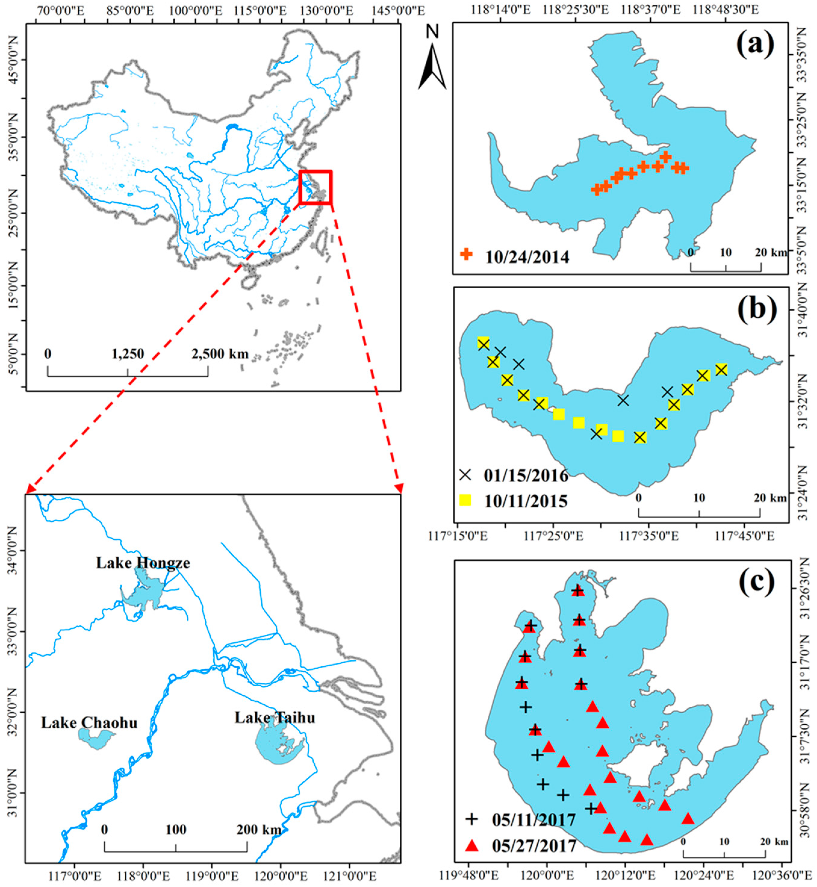
2.1.1. Study Area
2.1.2. Field Measurements
2.1.3. Satellite Data and Data Matching
2.2. Atmospheric Correction Algorithms
2.2.1. The Water-Atmospheric Correction Algorithms
2.2.2. The Land-Atmospheric Correction Algorithms
2.3. Water Type Classification
2.4. Statistical Indices
3. Results
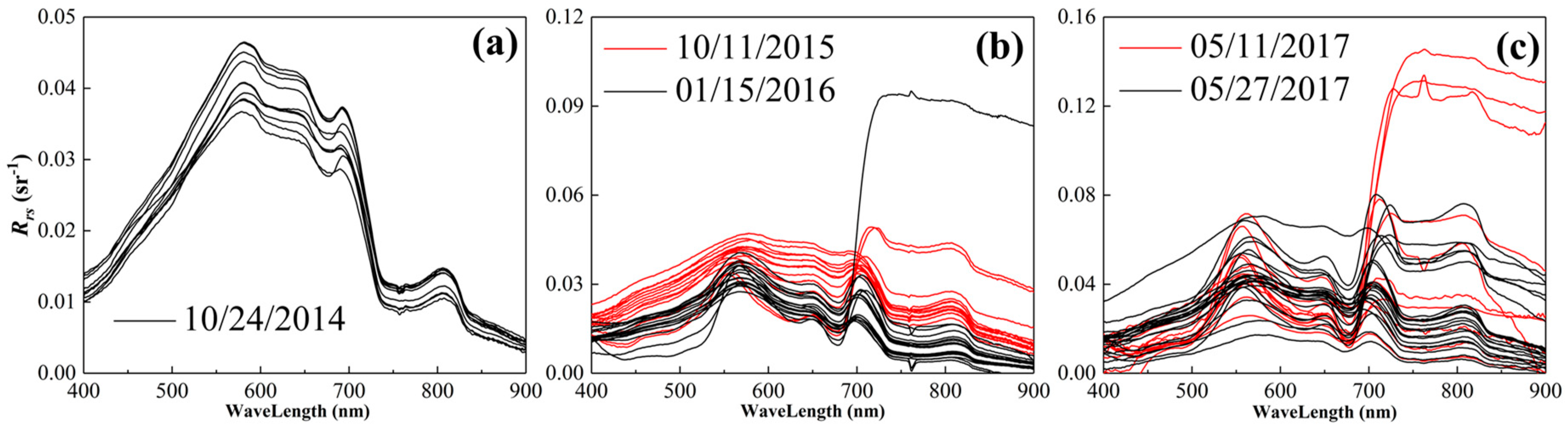
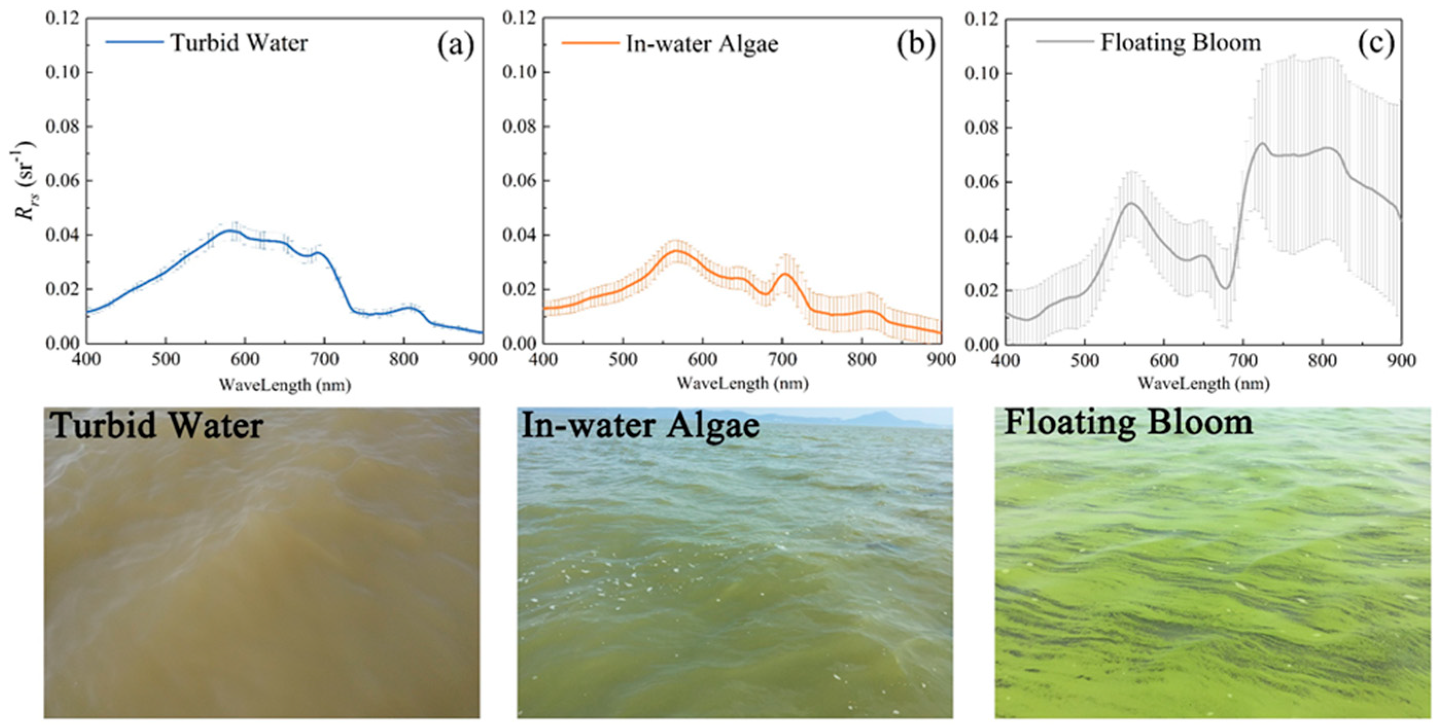
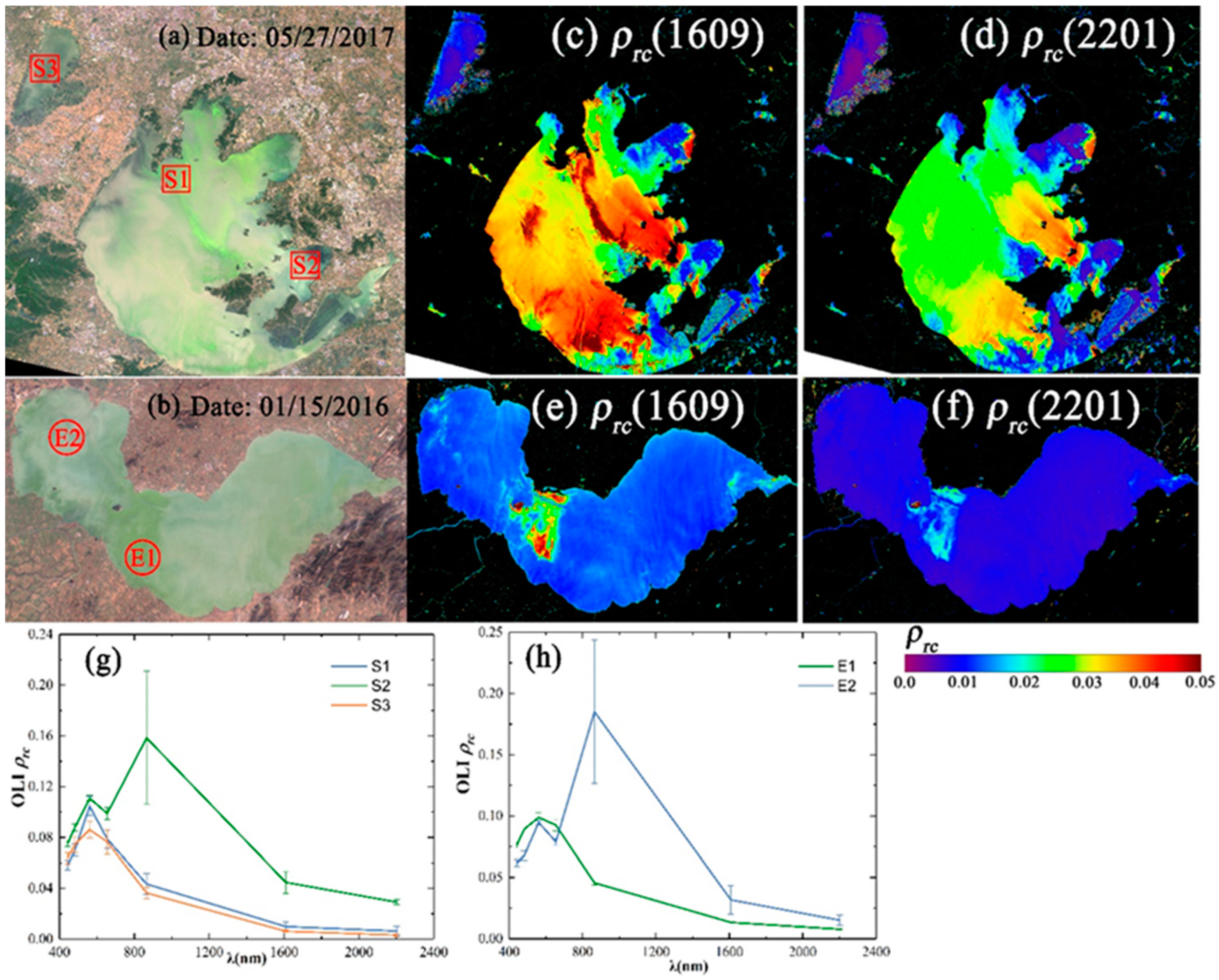
3.1. Spectrums and Water Conditions of Study Areas
3.2. Water Optical Properties and the Classification
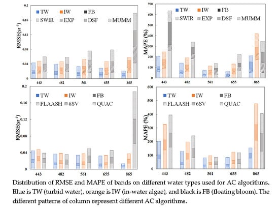
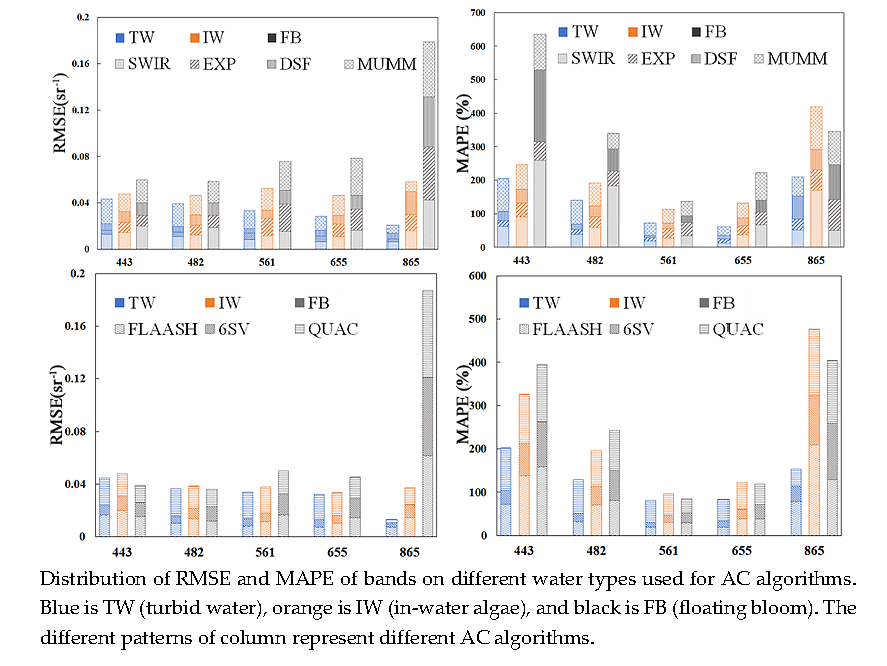
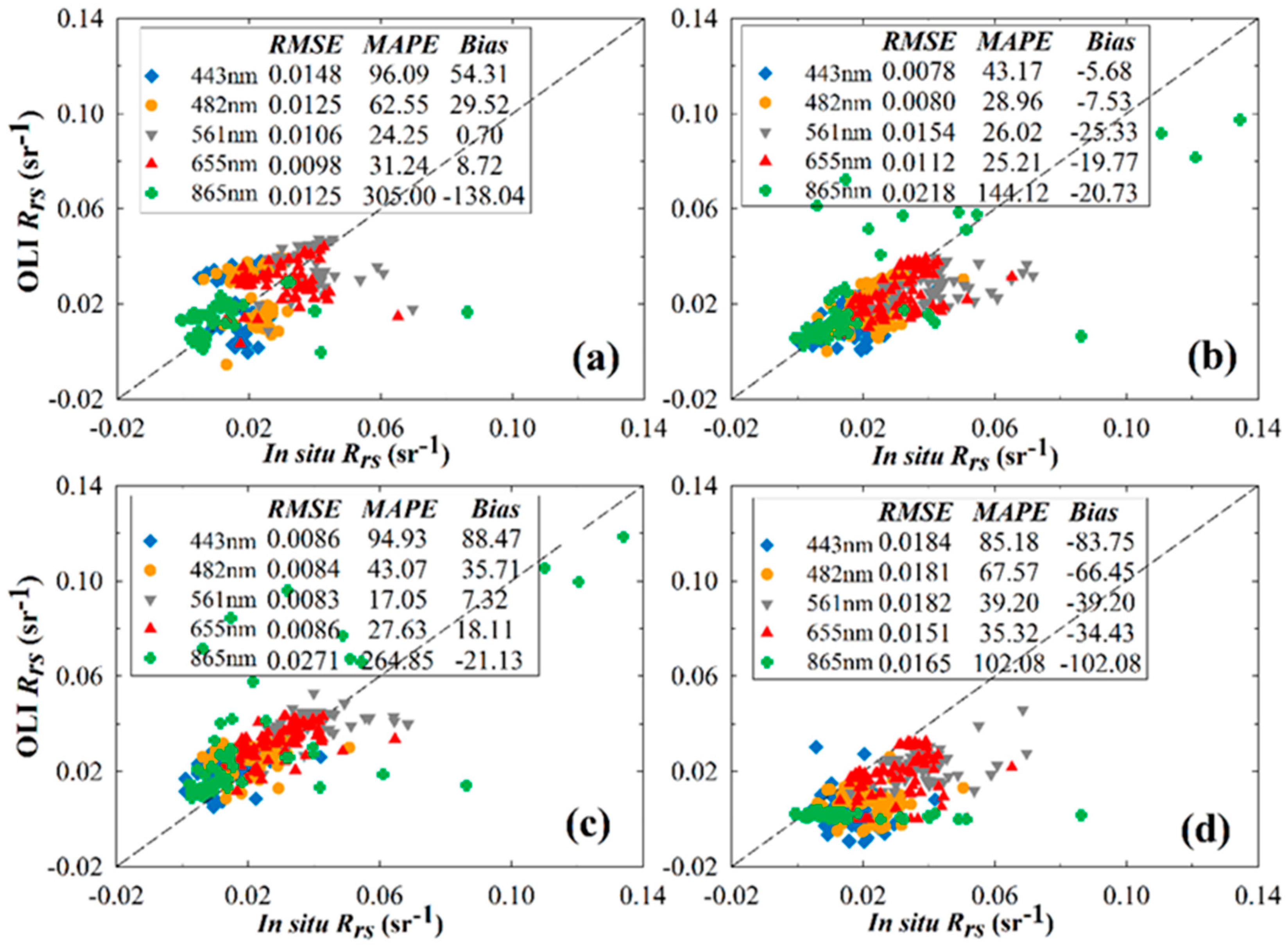
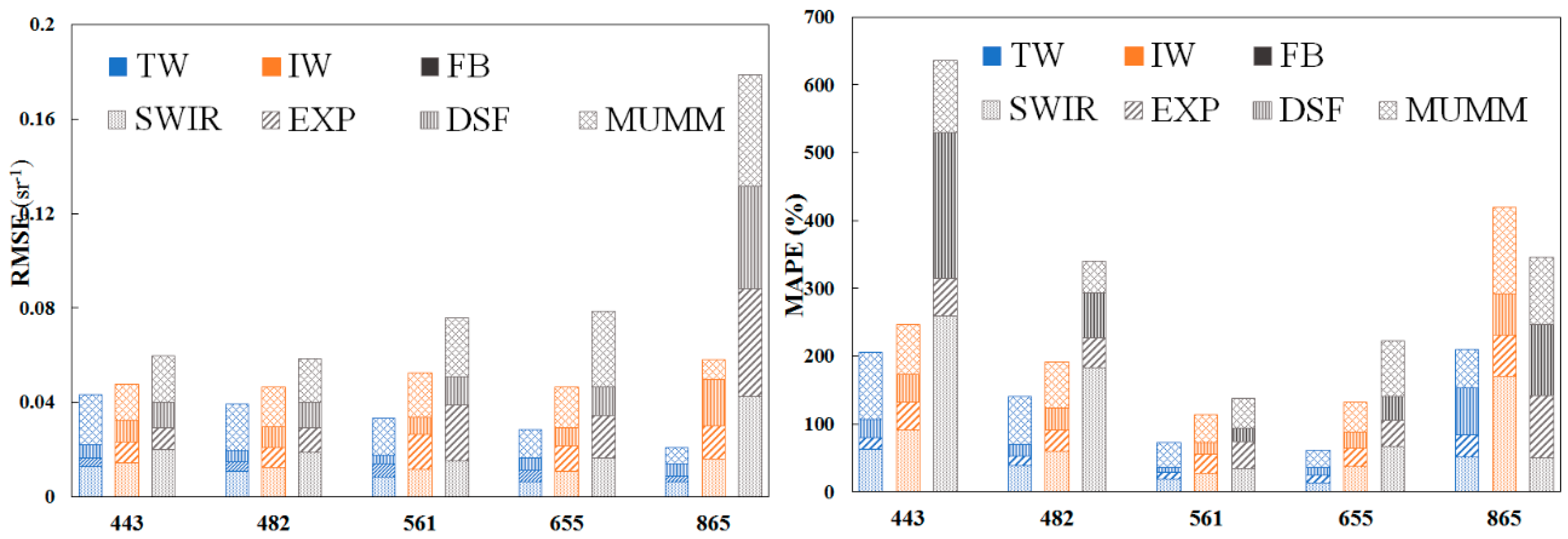
3.3. Assessment of the Water-AC Algorithms
3.3.1. Comparison with In Situ Measurements
3.3.2. Band Ratios
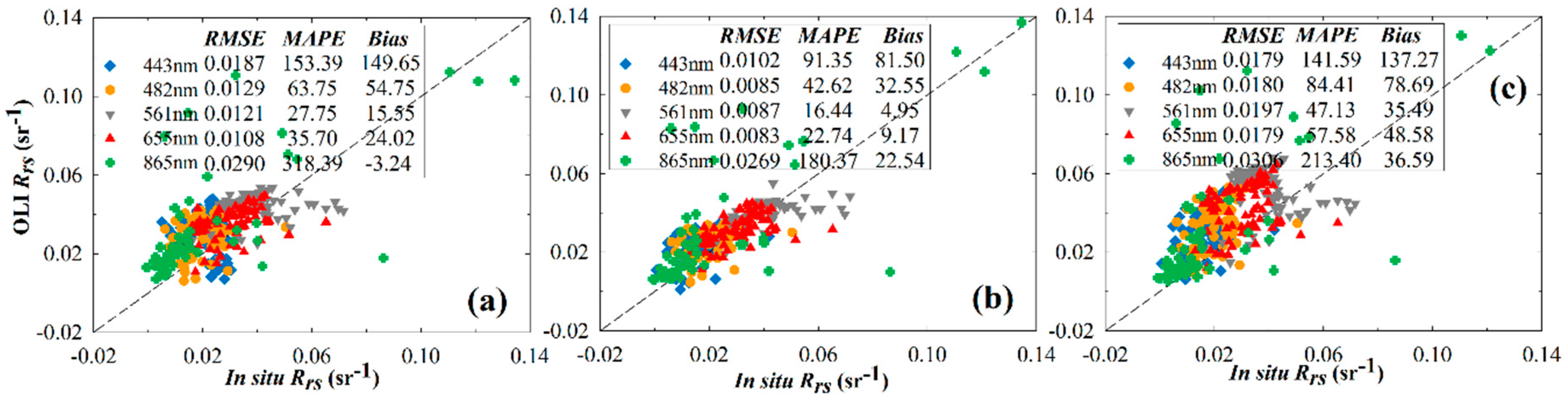
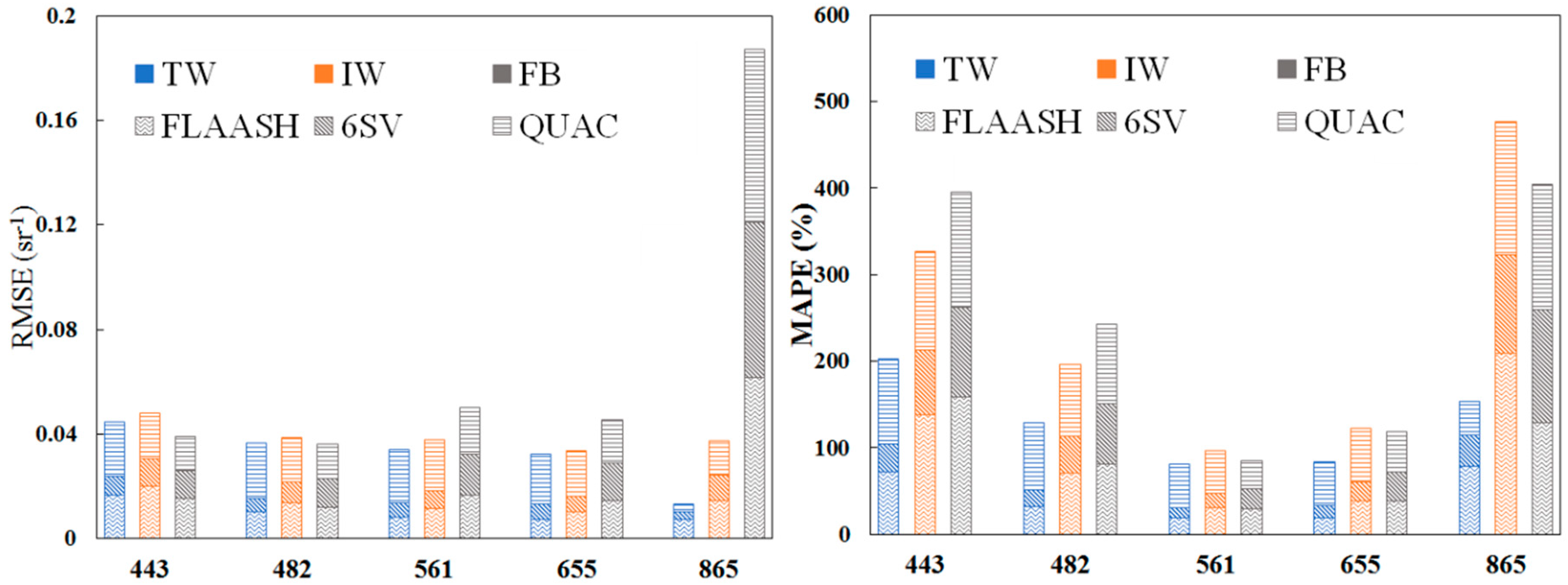
3.4. Assessment of the Land-AC Algorithms
3.4.1. Comparison with In Situ Measurements
3.4.2. Band Ratios
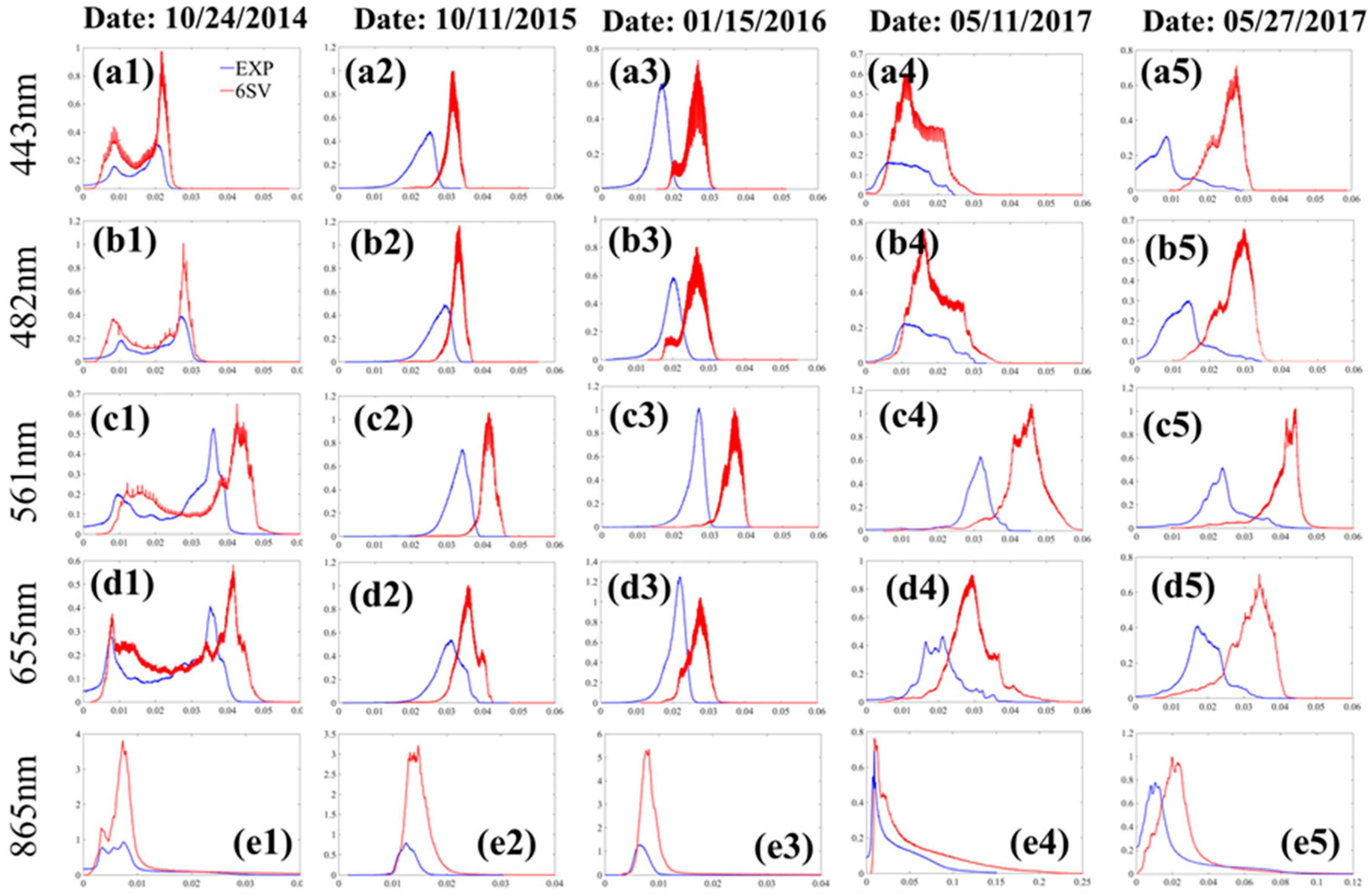
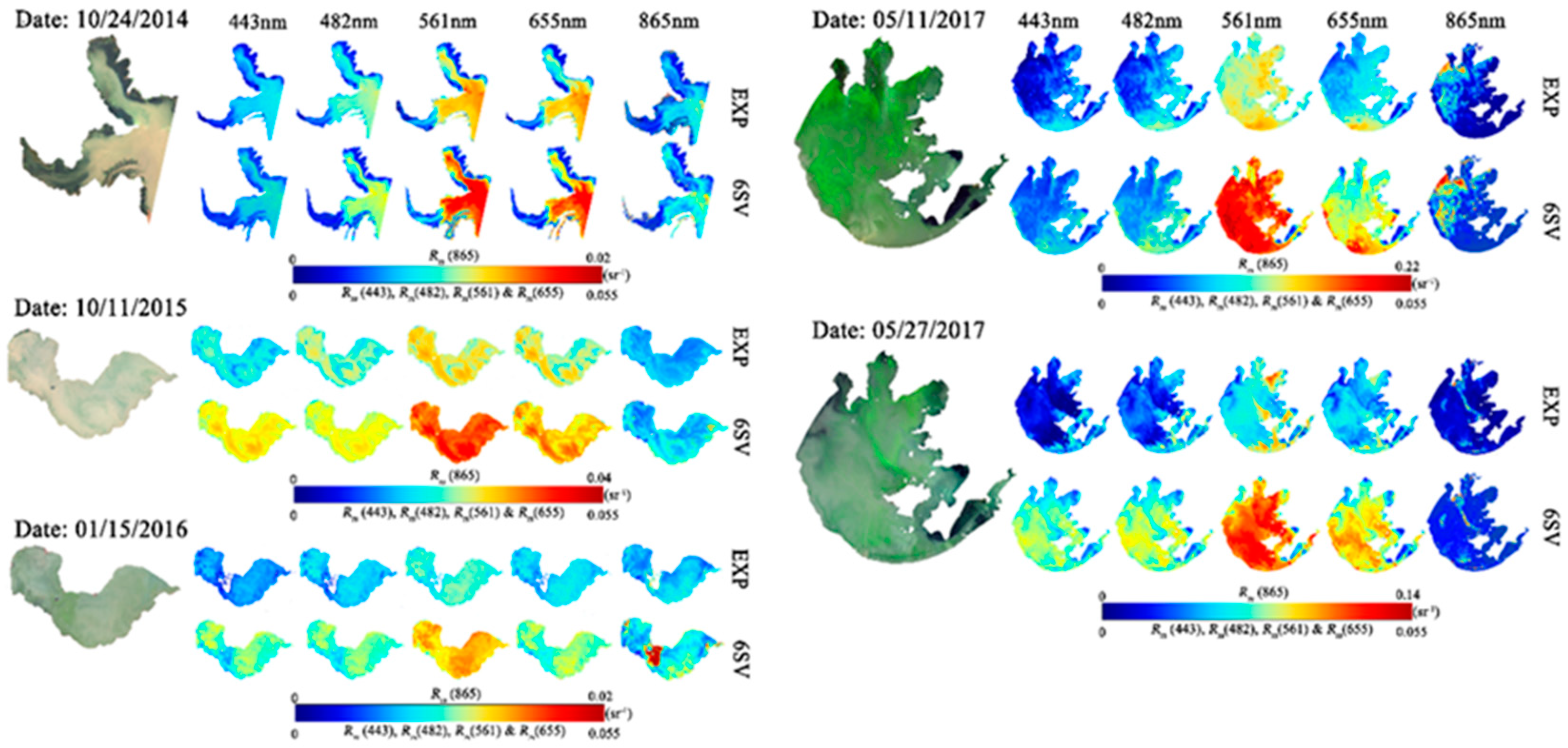
3.5. EXP vs. 6SV
3.5.1. Intercomparison of AC Algorithms
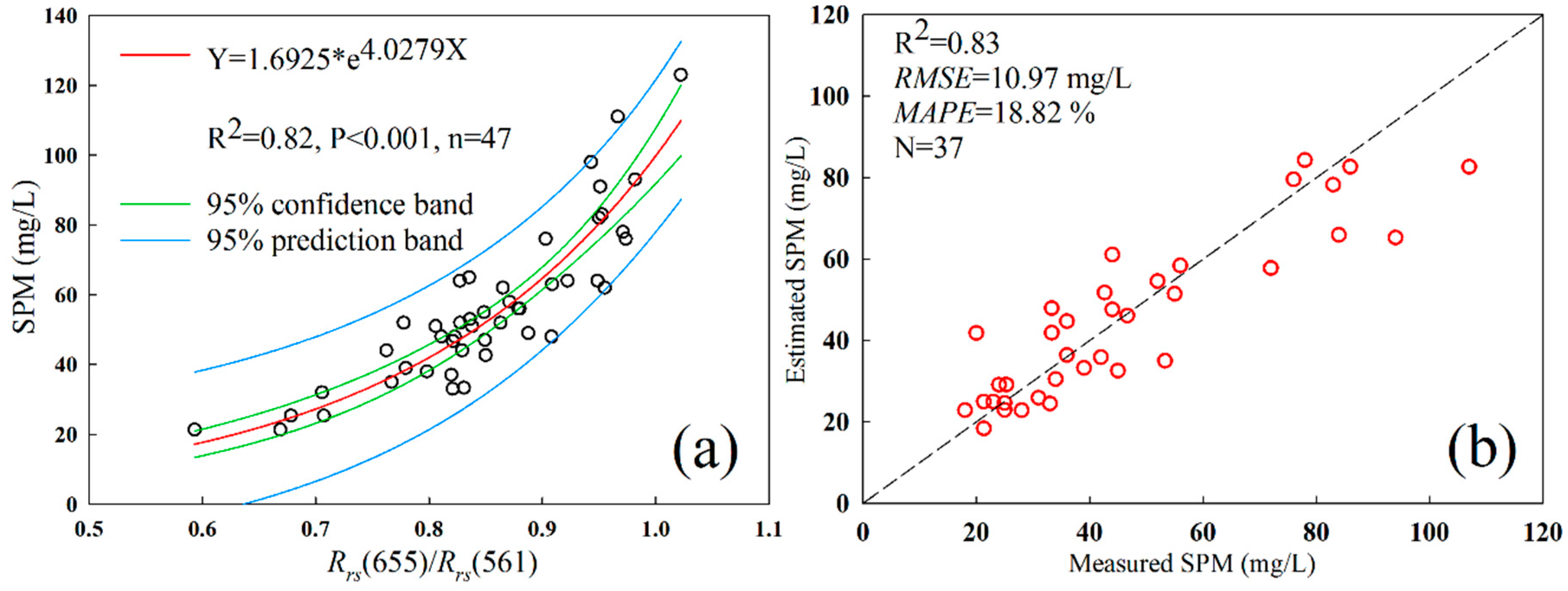
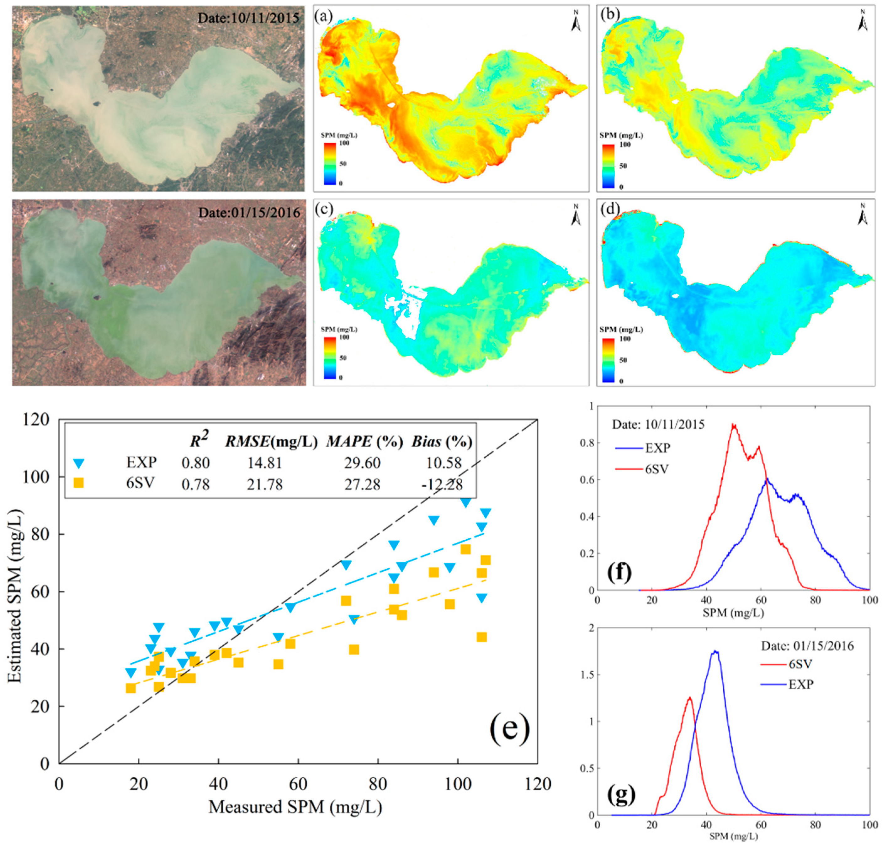
3.5.2. Performance of EXP and 6SV in SPM Estimation
4. Discussion
4.1. Assessment of AC Algorithms for Different Water Types
4.2. Does It Fit the “Black Pixel” Assumption?
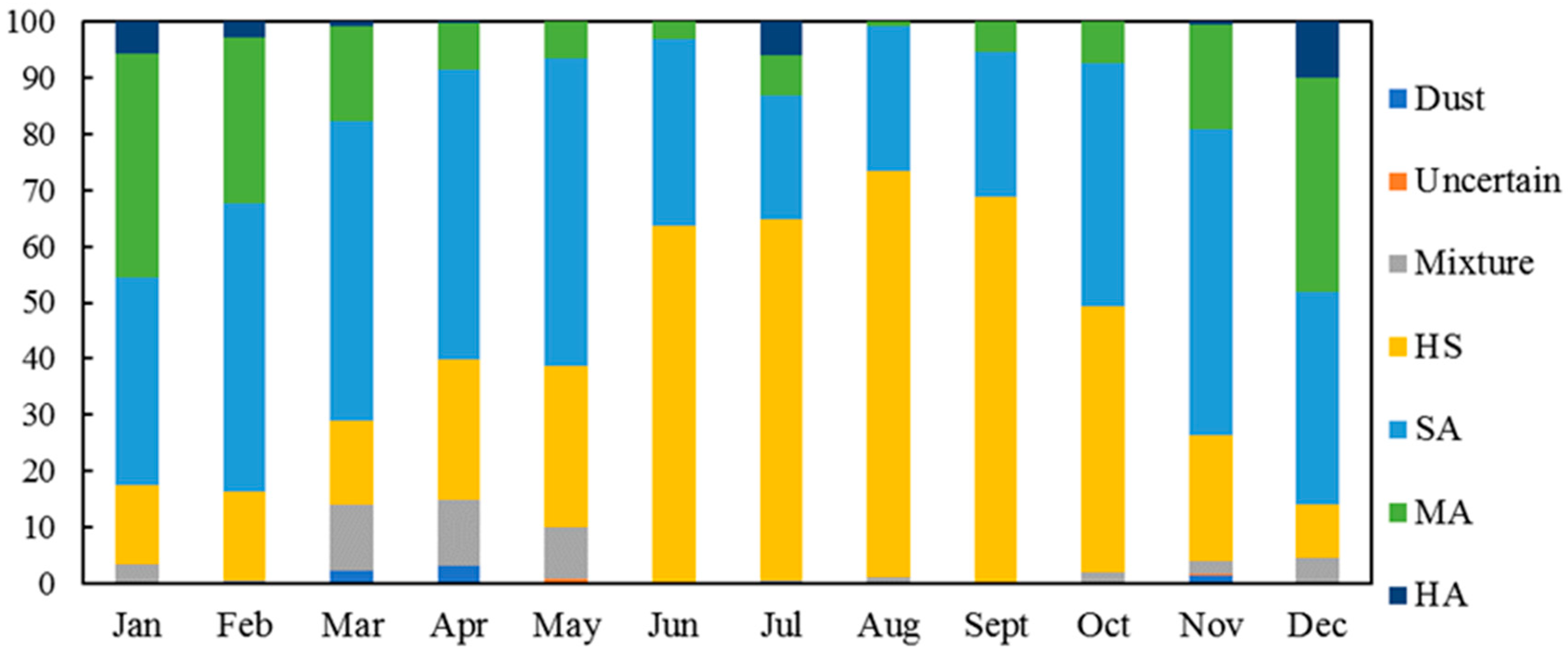
4.3. Does the Aerosol Model Accord with the Real Situation?
4.4. Validation of EXP Algorithm
5. Conclusions
Author Contributions
Funding
Acknowledgments
Conflicts of Interest
References
- Gordon, H.R. A Preliminary Assessment of the Nimbus-7 CZCS Atmospheric Correction Algorithm in a Horizontally Inhomogeneous Atmosphere. In Oceanography from Space; Gower, J.F.R., Ed.; Plenum Press: New York, NY, USA; London, UK, 1981; pp. 257–258. [Google Scholar]
- Wang, M. Atmospheric Correction for Remotely-Sensed OceanColour Products; International Ocean-Colour Coordinating Group: Monterey, CA, USA, 2010. [Google Scholar]
- Gordon, H.R.; Wang, M. Retrieval of water-leaving radiance and aerosol optical thickness over the oceans with SeaWiFS: A preliminary algorithm. Appl. Opt. 1994, 33, 443–452. [Google Scholar] [CrossRef] [PubMed]
- Siegel, D.A.; Wang, M.; Maritorena, S.; Robinson, W. Atmospheric correction of satellite ocean color imagery: The black pixel assumption. Appl. Opt. 2000, 39, 3582–3591. [Google Scholar] [CrossRef] [PubMed]
- Hu, C.; Carder, K.L.; Muller-Karger, F.E. Atmospheric Correction of SeaWiFS Imagery over Turbid Coastal Waters. Remote Sens. Environ. 2000, 74, 195–206. [Google Scholar] [CrossRef]
- Ruddick, K.G.; Ovidio, F.; Rijkeboer, M. Atmospheric correction of SeaWiFS imagery for turbid coastal and inland waters. Appl. Opt. 2000, 39, 897–912. [Google Scholar] [CrossRef] [PubMed]
- Wang, M.; Shi, W. Estimation of ocean contribution at the MODIS near-infrared wavelengths along the east coast of the U.S.: Two case studies. Geophys. Res. Lett. 2005, 32, L13606. [Google Scholar] [CrossRef]
- Ahmad, Z.; Franz, B.A.; McClain, C.R.; Kwiatkowska, E.J.; Werdell, J.; Shettle, E.P.; Holben, B.N. New aerosol models for the retrieval of aerosol optical thickness and normalized water-leaving radiances from the SeaWiFS and MODIS sensors over coastal regions and open oceans. Appl. Opt. 2010, 49, 5545–5560. [Google Scholar] [CrossRef] [PubMed]
- Hu, C.; Muller-Karger, F.E.; Andrefouet, S.; Carder, K.L. Atmospheric correction and cross-calibration of LANDSAT-7/ETM+ imagery over aquatic environments: A multiplatform approach using SeaWiFS/MODIS. Remote Sens. Environ. 2001, 78, 99–107. [Google Scholar] [CrossRef]
- Moses, W.J.; Gitelson, A.A.; Perk, R.L.; Gurlin, D.; Rundquist, D.C.; Leavitt, B.C.; Barrow, T.M.; Brakhage, P. Estimation of chlorophyll—A concentration in turbid productive waters using airborne hyperspectral data. Water Res. 2012, 46, 993–1004. [Google Scholar] [CrossRef] [PubMed]
- Lobo, F.L.; Costa, M.P.; Novo, E.M. Time-series analysis of Landsat-MSS/TM/OLI images over Amazonian waters impacted by gold mining activities. Remote Sens. Environ. 2015, 157, 170–184. [Google Scholar] [CrossRef]
- Allan, M.G.; Hamilton, D.P.; Hicks, B.J.; Brabyn, L. Landsat remote sensing of chlorophyllaconcentrations in central North Island lakes of New Zealand. Int. J. Remote Sens. 2011, 32, 2037–2055. [Google Scholar] [CrossRef]
- Tan, J.; Cherkauer, K.A.; Chaubey, I.; Troy, C.D.; Essig, R. Water quality estimation of River plumes in Southern Lake Michigan using Hyperion. J. Great Lakes Res. 2016, 42, 524–535. [Google Scholar] [CrossRef]
- Anderson, G.P.; Felde, G.W.; Hoke, M.L.; Ratkowski, A.J.; Cooley, T.W.; James, H.; Chetwynd, J.; Gardner, J.A.; Adler-Golden, S.M.; Matthew, M.W.; et al. MODTRAN4-based atmospheric correction algorithm: FLAASH (fast line-of-sight atmospheric analysis of spectral hypercubes). Proc. SPIE-Int. Soc. Opt. Eng. 2002, 4725, 65–71. [Google Scholar] [CrossRef]
- Vermote, E.F.; Tanré, D.; Deuzé, J.L.; Herman, M.; Morcrette, J.J.; Kotchenova, S.Y. Second Simulation of a Satellite Signal in the Solar Spectrum-Vector (6SV); University of Maryland: College Park, MD, USA, 2006. [Google Scholar]
- Carr, S.B.; Bernstein, L.S.; Adler-Golden, S.M. The Quick Atmospheric Correction (QUAC) Algorithm for Hyperspectral Image Processing: Extending QUAC to a Coastal Scene. In Proceedings of the 2015 International Conference Digital Image Computing: Techniques and Applications, Adelaide, Australia, 23–25 November 2015. [Google Scholar]
- Bernstein, L.S.; Lewis, P.E.; Adler-Golden, S.M.; Sundberg, R.L.; Levine, R.Y.; Perkins, T.C.; Berk, A.; Ratkowski, A.J.; Felde, G.; Hoke, M.L. Validation of the QUick atmospheric correction (QUAC) algorithm for VNIR-SWIR multi- and hyperspectral imagery. Proc. SPIE-Int. Soc. Opt. Eng. 2005, 5806, 668–678. [Google Scholar] [CrossRef]
- Knight, E.; Kvaran, G. Landsat-8 Operational Land Imager Design, Characterization and Performance. Remote Sens. 2014, 6, 10286–10305. [Google Scholar] [CrossRef]
- Concha, J.A.; Schott, J.R. Retrieval of color producing agents in Case 2 waters using Landsat 8. Remote Sens. Environ. 2016, 185, 95–107. [Google Scholar] [CrossRef]
- Pahlevan, N.; Lee, Z.; Wei, J.; Schaaf, C.B.; Schott, J.R.; Berk, A. On-orbit radiometric characterization of OLI (Landsat-8) for applications in aquatic remote sensing. Remote Sens. Environ. 2014, 154, 272–284. [Google Scholar] [CrossRef]
- Barsi, J.; Lee, K.; Kvaran, G.; Markham, B.; Pedelty, J. The Spectral Response of the Landsat-8 Operational Land Imager. Remote Sens. 2014, 6, 10232–10251. [Google Scholar] [CrossRef]
- Mushtaq, F.; Nee Lala, M.G. Remote estimation of water quality parameters of Himalayan lake (Kashmir) using Landsat 8 OLI imagery. Geocarto Int. 2016, 32, 274–285. [Google Scholar] [CrossRef]
- Zheng, Z.; Ren, J.; Li, Y.; Huang, C.; Liu, G.; Du, C.; Lyu, H. Remote sensing of diffuse attenuation coefficient patterns from Landsat 8 OLI imagery of turbid inland waters: A case study of Dongting Lake. Sci. Total Environ. 2016, 573, 39–54. [Google Scholar] [CrossRef]
- Vanhellemont, Q.; Ruddick, K. Turbid wakes associated with offshore wind turbines observed with Landsat 8. Remote Sens. Environ. 2014, 145, 105–115. [Google Scholar] [CrossRef]
- Vanhellemont, Q.; Ruddick, K. Advantages of high quality SWIR bands for ocean colour processing: Examples from Landsat-8. Remote Sens. Environ. 2015, 161, 89–106. [Google Scholar] [CrossRef]
- Vanhellemont, Q.; Ruddick, K. Atmospheric correction of metre-scale optical satellite data for inland and coastal water applications. Remote Sens. Environ. 2018, 216, 586–597. [Google Scholar] [CrossRef]
- Irons, J.R.; Dwyer, J.L.; Barsi, J.A. The next Landsat satellite: The Landsat Data Continuity Mission. Remote Sens. Environ. 2012, 122, 11–21. [Google Scholar] [CrossRef]
- Ma, R.; Dai, J. Investigation of chlorophyll—A and total suspended matter concentrations using Landsat ETM and field spectral measurement in Taihu Lake, China. Int. J. Remote Sens. 2005, 26, 2779–2795. [Google Scholar] [CrossRef]
- Duan, H.; Tao, M.; Loiselle, S.A.; Zhao, W.; Cao, Z.; Ma, R.; Tang, X. MODIS observations of cyanobacterial risks in a eutrophic lake: Implications for long-term safety evaluation in drinking-water source. Water Res. 2017, 122, 455–470. [Google Scholar] [CrossRef] [PubMed]
- Hu, C.; Lee, Z.; Ma, R.; Yu, K.; Li, D.; Shang, S. Moderate Resolution Imaging Spectroradiometer (MODIS) observations of cyanobacteria blooms in Taihu Lake, China. J. Geophys. Res. 2010, 115, C04002. [Google Scholar] [CrossRef]
- Mueller, J.L.; Fargion, G.S.; McClain, C.R. Ocean Optics Protocols for Satellite Ocean Color Sensor Validation, Revision 5, Volume V: Biogeochemical and Bio-Optical Measurements and Data Analysis Protocols; NASA Tech: Washington, DC, USA, 2003. [Google Scholar]
- Mobley, C.D. Estimation of the remote-sensing reflectance from above-surface measurements. Appl. Opt. 1999, 38, 7442–7455. [Google Scholar]
- Hu, L.; Hu, C.; Ming-Xia, H. Remote estimation of biomass of Ulva prolifera macroalgae in the Yellow Sea. Remote Sens. Environ. 2017, 192, 217–227. [Google Scholar] [CrossRef]
- Gitelson, A.A.; Dall’Olmo, G.; Moses, W.; Rundquist, D.C.; Barrow, T.; Fisher, T.R.; Gurlin, D.; Holz, J. A simple semi-analytical model for remote estimation of chlorophyll—A in turbid waters: Validation. Remote Sens. Environ. 2008, 112, 3582–3593. [Google Scholar] [CrossRef]
- Werdell, P.J.; Franz, B.A.; Bailey, S.W.; Feldman, G.C.; Boss, E.; Brando, V.E.; Dowell, M.; Hirata, T.; Lavender, S.J.; Lee, Z.; et al. Generalized ocean color inversion model for retrieving marine inherent optical properties. Appl Opt 2013, 52, 2019–2037. [Google Scholar] [CrossRef]
- Qi, H.; Lu, J.; Chen, X.; Sauvage, S.; Sanchez-Perez, J.-M. Water age prediction and its potential impacts on water quality using a hydrodynamic model for Poyang Lake, China. Environ. Sci. Pollut. Res. Int. 2016, 23, 13327–13341. [Google Scholar] [CrossRef] [PubMed]
- Ma, R.-H.; Tang, J.-W.; Dai, J.-F. Bio-optical model with optimal parameter suitable for Taihu Lake in water colour remote sensing. Int. J. Remote Sens. 2006, 27, 4305–4328. [Google Scholar] [CrossRef]
- Mitchell, B.G. Algorithms for determining the absorption-coefficient of aquatic particulates using the Quantitative Filter Technique. Proc. SPIE-Int. Soc. Opt. Eng. 1990, 1302, 132–148. [Google Scholar]
- Pope, R.M.; Fry, E.S. Absorption spectrum (380–700 nm) of pure water. II. Integrating cavity measurements. Appl. Opt. 1997, 36, 8710–8723. [Google Scholar] [CrossRef]
- Xue, K.; Zhang, Y.; Duan, H.; Ma, R. Variability of light absorption properties in optically complex inland waters of Lake Chaohu, China. J. Great Lakes Res. 2017, 43, 17–31. [Google Scholar] [CrossRef]
- Cao, Z.; Duan, H.; Feng, L.; Ma, R.; Xue, K. Climate- and human-induced changes in suspended particulate matter over Lake Hongze on short and long timescales. Remote Sens. Environ. 2017, 192, 98–113. [Google Scholar] [CrossRef]
- Franz, B.A.; Bailey, S.W.; Kuring, N.; Werdell, P.J. Ocean color measurements with the Operational Land Imager on Landsat-8: Implementation and evaluation in SeaDAS. J. Appl. Remote Sens. 2015, 9, 096070. [Google Scholar] [CrossRef]
- Pahlevan, N.; Roger, J.C.; Ahmad, Z. Revisiting short-wave-infrared (SWIR) bands for atmospheric correction in coastal waters. Opt. Express 2017, 25, 6015–6035. [Google Scholar] [CrossRef]
- Hale, G.M.; Querry, M.R. Optical constants of water in the 200 nm to 200 µm wavelength region. Appl. Opt. 1973, 12, 555–563. [Google Scholar] [CrossRef]
- Shi, W.; Wang, M. An assessment of the black ocean pixel assumption for MODIS SWIR bands. Remote Sens. Environ. 2009, 113, 1587–1597. [Google Scholar] [CrossRef]
- Ruddick, K.G. Seaborne measurements of near infrared water-leaving reflectance: The similarity spectrum for turbid waters. Limnol. Oceanogr. 2006, 51, 1167–1179. [Google Scholar] [CrossRef]
- Ruddick, K.G.; Gons, H.J.; Rijkeboer, M.; Tilstone, G. Optical remote sensing of chlorophyll a in case 2 waters by use of an adaptive two-band algorithm with optimal error properties. Appl. Opt. 2001, 40, 3575–3584. [Google Scholar] [CrossRef] [PubMed]
- Jamet, C.; Loisel, H.; Kuchinke, C.P.; Ruddick, K.; Zibordi, G.; Feng, H. Comparison of three SeaWiFS atmospheric correction algorithms for turbid waters using AERONET-OC measurements. Remote Sens. Environ. 2011, 115, 1955–1965. [Google Scholar] [CrossRef]
- Vanhellemont, Q. Atmospheric correction of Landsat-8 imagery using SeaDAS. In Proceedings of the 2014 European Space Agency Sentinel-2 for Science Workshop, Frascati, Italy, 20–22 May 2014. [Google Scholar]
- Chavez, P.S., Jr. An Improved Dark-Object Subtraction Technique for Atmospheric Scattering Correction of Multispectral Data. Remote Sens. Environ. 1988, 24, 459–479. [Google Scholar] [CrossRef]
- Liu, G.; Li, Y.; Lyu, H.; Wang, S.; Du, C.; Huang, C. An Improved Land Target-Based Atmospheric Correction Method for Lake Taihu. IEEE J. Sel. Top. Appl. Earth Obs. Remote Sens. 2016, 9, 793–803. [Google Scholar] [CrossRef]
- Kaufman, Y.J.; Sendra, C. Algorithm for automatic atmospheric corrections to visible and near-IR satellite imagery. Int. J. Remote Sens. 1988, 9, 1357–1381. [Google Scholar] [CrossRef]
- Bernstein, L.S. Quick atmospheric correction code: Algorithm description and recent upgrades. Opt. Eng. 2012, 51, 111719. [Google Scholar] [CrossRef]
- Yu, K.; Liu, S.; Zhao, Y. CPBAC: A quick atmospheric correction method using the topographic information. Remote Sens. Environ. 2016, 186, 262–274. [Google Scholar] [CrossRef]
- Kudela, R.M.; Palacios, S.L.; Austerberry, D.C.; Accorsi, E.K.; Guild, L.S.; Torres-Perez, J. Application of hyperspectral remote sensing to cyanobacterial blooms in inland waters. Remote Sens. Environ. 2015, 167, 196–205. [Google Scholar] [CrossRef]
- Yang, Y.; Liu, Y.; Zhou, M.; Zhang, S.; Zhan, W.; Sun, C.; Duan, Y. Landsat 8 OLI image based terrestrial water extraction from heterogeneous backgrounds using a reflectance homogenization approach. Remote Sens. Environ. 2015, 171, 14–32. [Google Scholar] [CrossRef]
- Wei, J.; Lee, Z.; Garcia, R.; Zoffoli, L.; Armstrong, R.A.; Shang, Z.; Sheldon, P.; Chen, R.F. An assessment of Landsat-8 atmospheric correction schemes and remote sensing reflectance products in coral reefs and coastal turbid waters. Remote Sens. Environ. 2018, 215, 18–32. [Google Scholar] [CrossRef]
- Kaufman, Y.J.; Wald, A.E.; Remer, L.A.; Gao, B.-C.; Li, R.-R.; Flynn, L. The MODIS 2.1 μm channel—Correlation with visible reflectance for use in remote sensing of aerosol. Geosci. Remote Sens. 1997, 35, 1286–1298. [Google Scholar] [CrossRef]
- Rotta, L.H.S.; Alcântara, E.H.; Watanabe, F.S.Y.; Rodrigues, T.W.P.; Imai, N.N. Atmospheric correction assessment of SPOT-6 image and its influence on models to estimate water column transparency in tropical reservoir. Remote Sens. Appl. Soc. Environ. 2016, 4, 158–166. [Google Scholar] [CrossRef]
- Vermote, E.F.; Member, I.; Tan, D.; Deuze, J.L.; Herman, M. Second Simulation of the Satellite Signal in the Solar Spectrum, 6s: An Overview. IEEE Trans. Geosci. Remote Sens. 1997, 35, 675–687. [Google Scholar] [CrossRef]
- Kotchenova, S.Y.; Vermote, E.F. Validation of a vector version of the 6S radiative transfer code for atmospheric correction of satellite data. Part II: Homogeneous Lambertian and anisotropic surfaces. Appl. Opt. 2007, 46, 4455–4464. [Google Scholar] [CrossRef] [PubMed]
- Tachiiri, K. Calculating NDVI for NOAA/AVHRR data after atmospheric correction for extensive images using 6S code: A case study in the Marsabit District, Kenya. ISPRS J. Photogramm. Remote Sens. 2005, 59, 103–114. [Google Scholar] [CrossRef]
- Shen, M.; Duan, H.; Cao, Z.; Xue, K.; Loiselle, S.; Yesou, H. Determination of the Downwelling Diffuse Attenuation Coefficient of Lake Water with the Sentinel-3A OLCI. Remote Sens. 2017, 9, 1246. [Google Scholar] [CrossRef]
- Sun, D.; Li, Y.; Wang, Q.; Le, C.; Lv, H.; Huang, C.; Gong, S. Specific inherent optical quantities of complex turbid inland waters, from the perspective of water classification. Photochem. Photobiol. Sci. 2012, 11, 1299–1312. [Google Scholar] [CrossRef]
- Wu, J.L.; Ho, C.R.; Huang, C.C.; Srivastav, A.L.; Tzeng, J.H.; Lin, Y.T. Hyperspectral sensing for turbid water quality monitoring in freshwater rivers: Empirical relationship between reflectance and turbidity and total solids. Sensors 2014, 14, 22670–22688. [Google Scholar] [CrossRef]
- Pham, Q.; Ha, N.; Pahlevan, N.; Oanh, L.; Nguyen, T.; Nguyen, N. Using Landsat-8 Images for Quantifying Suspended Sediment Concentration in Red River (Northern Vietnam). Remote Sens. 2018, 10, 1841. [Google Scholar] [CrossRef]
- Anderson, G.P.; Pukall, B.; Allred, C.L.; Matthew, M.W. FLAASH and MODTRAN4: State-of-the-art atmospheric correction for hyperspectral data. Conf. Aerosp. Conf. 1999, 4, 177–181. [Google Scholar]
- Lee, J.; Kim, J.; Song, C.H.; Kim, S.B.; Chun, Y.; Sohn, B.J.; Holben, B.N. Characteristics of aerosol types from AERONET sunphotometer measurements. Atmos. Environ. 2010, 44, 3110–3117. [Google Scholar] [CrossRef]
- Wang, M. A Simple, Moderately Accurate, Atmospheric correction algorithn for SeaWiFS. Remote Sens. Environ. 1994, 50, 231–239. [Google Scholar] [CrossRef]
- Caballero, I.; Navarro, G.; Ruiz, J. Multi-platform assessment of turbidity plumes during dredging operations in a major estuarine system. Int. J. Appl. Earth Obs. Geoinf. 2018, 68, 31–41. [Google Scholar] [CrossRef]
- Lee, Z.; Shang, S.; Qi, L.; Yan, J.; Lin, G. A semi-analytical scheme to estimate Secchi-disk depth from Landsat-8 measurements. Remote Sens. Environ. 2016, 177, 101–106. [Google Scholar] [CrossRef]
- Novoa, S.; Doxaran, D.; Ody, A.; Vanhellemont, Q.; Lafon, V.; Lubac, B.; Gernez, P. Atmospheric Corrections and Multi-Conditional Algorithm for Multi-Sensor Remote Sensing of Suspended Particulate Matter in Low-to-High Turbidity Levels Coastal Waters. Remote Sens. 2017, 9, 61. [Google Scholar] [CrossRef]
- Li, J.; Yu, Q.; Tian, Y.Q.; Becker, B.L.; Siqueira, P.; Torbick, N. Spatio-temporal variations of CDOM in shallow inland waters from a semi-analytical inversion of Landsat-8. Remote Sens. Environ. 2018, 218, 189–200. [Google Scholar] [CrossRef]


| Band | Band Range (nm) | Band Center (nm) | GSD (m) | SNR at Reference L |
|---|---|---|---|---|
| Band1 Coastal/Aerosol | 433–453 | 443 | 30 | 232 |
| Band 2 Blue | 450–515 | 482 | 30 | 355 |
| Band 3 Green | 525–600 | 561 | 30 | 296 |
| Band 4 Red | 630–680 | 655 | 30 | 222 |
| Band 5 NIR | 845–885 | 865 | 30 | 199 |
| Band 6 SWIR 1 | 1560–1660 | 1609 | 30 | 261 |
| Band 7 SWIR 2 | 2100–2300 | 2201 | 30 | 326 |
| Band 8 Pan | 500–680 | 590 | 15 | 146 |
| Band 9 Cirrus | 1360–1390 | 1375 | 30 | 162 |
| OLI Image | Acquisition Date | in situ Number | |
|---|---|---|---|
| Lake Hongze | LC81210372014297 | 24 October 2014 | 10 |
| Lake Chaohu | LC81210382015284 | 11 October 2015 | 15 |
| LC81210382016015 | 15 January 2016 | 16 | |
| Lake Taihu | LC81190382017131 | 11 May 2017 | 11 |
| LC81190382017147 | 27 May 2017 | 22 |
| Lake | Parameters | Minimum | Maximum | Mean | SD |
|---|---|---|---|---|---|
| Lake Hongze (n = 10) | Chla | 7.35 | 19.21 | 11.62 | 3.33 |
| SPOM | 6.00 | 11.33 | 8.67 | 1.61 | |
| SPIM | 28.00 | 47.33 | 35.33 | 6.68 | |
| SPOM/SPIM | 0.16 | 0.40 | 0.25 | 0.07 | |
| ag(440) | 1.19 | 1.59 | 1.38 | 0.13 | |
| aph(665) | 0.16 | 0.25 | 0.19 | 0.03 | |
| Lake Chaohu (n = 31) | Chla | 9.86 | 687.14 | 140.68 | 184.01 |
| SPOM | 8.00 | 216.00 | 38.53 | 48.08 | |
| SPIM | 8.00 | 93.00 | 40.94 | 27.93 | |
| SPOM/SPIM | 0.15 | 9.82 | 1.39 | 1.94 | |
| ag(440) | 0.79 | 1.75 | 1.22 | 0.27 | |
| aph(665) | 0.13 | 8.48 | 1.31 | 1.81 | |
| Lake Taihu (n = 33) | Chla | 19.96 | 1022.53 | 206.13 | 267.93 |
| SPOM | 4.00 | 321.33 | 72.04 | 85.48 | |
| SPIM | 13.33 | 88.00 | 44.14 | 16.80 | |
| SPOM/SPIM | 0.12 | 6.51 | 1.67 | 1.76 | |
| ag(440) | 0.46 | 3.28 | 1.16 | 0.60 | |
| aph(665) | 0.34 | 26.95 | 3.48 | 5.80 |
| Lake | Parameters | Minimum | Maximum | Mean | SD |
|---|---|---|---|---|---|
| Turbid water (n = 20) | Chla | 7.35 | 91.72 | 28.10 | 22.57 |
| SPOM | 6.00 | 34.00 | 14.77 | 8.09 | |
| SPIM | 28.00 | 93.00 | 52.44 | 20.34 | |
| SPOM/SPIM | 0.12 | 0.47 | 0.28 | 0.10 | |
| ag(440) | 0.89 | 1.75 | 1.36 | 0.24 | |
| aph(665) | 0.13 | 0.92 | 0.29 | 0.21 | |
| In-water algae (n = 38) | Chla | 19.96 | 687.14 | 104.39 | 125.78 |
| SPOM | 4.00 | 226.67 | 44.29 | 44.35 | |
| SPIM | 8.00 | 68.00 | 28.18 | 17.52 | |
| SPOM/SPIM | 0.23 | 8.67 | 1.57 | 1.96 | |
| ag(440) | 0.46 | 1.75 | 1.07 | 0.31 | |
| aph(665) | 0.31 | 16.43 | 1.89 | 3.01 | |
| Floating bloom (n = 16) | Chla | 103.86 | 1022.53 | 198.04 | 203.85 |
| SPOM | 25.33 | 321.33 | 117.27 | 69.46 | |
| SPIM | 16.00 | 88.00 | 44.91 | 20.17 | |
| SPOM/SPIM | 0.40 | 9.82 | 2.61 | 2.50 | |
| ag(440) | 0.37 | 3.28 | 2.62 | 1.04 | |
| aph(665) | 0.32 | 26.95 | 6.59 | 8.07 |
| Algorithm | Band Ratio | |||||||
|---|---|---|---|---|---|---|---|---|
| 443/561 | 482/561 | 655/561 | 865/561 | 443/655 | 482/655 | 865/655 | ||
| SWIR | RMSE | 0.3125 | 0.2180 | 0.0915 | 0.3916 | 0.3538 | 0.2339 | 0.7163 |
| MAPE (%) | 69.91 | 37.35 | 10.50 | 227.69 | 59.95 | 30.15 | 201.77 | |
| Bias (%) | 37.62 | 20.16 | 6.30 | −88.12 | 27.24 | 11.80 | −71.86 | |
| EXP | RMSE | 0.1758 | 0.1694 | 0.0971 | 0.7781 | 0.2099 | 0.1645 | 1.5130 |
| MAPE (%) | 54.48 | 30.93 | 10.65 | 197.08 | 46.11 | 21.59 | 195.52 | |
| Bias (%) | 24.72 | 21.20 | 6.53 | 42.88 | 15.10 | 12.60 | 63.03 | |
| DSF | RMSE | 0.19 | 0.1577 | 0.0984 | 0.6372 | 0.1951 | 0.1406 | 1.0799 |
| MAPE (%) | 88.91 | 29.31 | 11.31 | 130.87 | 61.72 | 17.23 | 132.07 | |
| Bias (%) | 85.08 | 26.18 | 8.06 | 120.54 | 59.08 | 15.00 | 118.22 | |
| MUMM | RMSE | 0.5013 | 0.3888 | 0.1656 | 0.4601 | 0.7234 | 0.5489 | - |
| MAPE (%) | 91.19 | 57.73 | 17.54 | 89.43 | 101.08 | 63.13 | - | |
| Bias (%) | −86.60 | −53.97 | 4.36 | −89.28 | −97.62 | −60.88 | - | |
| Algorithm | Band Ratio | |||||||
|---|---|---|---|---|---|---|---|---|
| 443/561 | 482/561 | 655/561 | 865/561 | 443/655 | 482/655 | 865/655 | ||
| FLAASH | RMSE | 0.3422 | 0.1876 | 0.0861 | 0.6970 | 0.3994 | 0.1908 | 1.1892 |
| MAPE (%) | 131.05 | 34.72 | 9.85 | 237.69 | 108.43 | 24.52 | 229.94 | |
| Bias (%) | 129.99 | 30.50 | 6.16 | 35.80 | 108.10 | 21.24 | 51.04 | |
| 6SV | RMSE | 0.2363 | 0.1697 | 0.0774 | 0.6360 | 0.2885 | 0.1907 | 1.1338 |
| MAPE (%) | 84.97 | 30.49 | 8.26 | 162.83 | 72.14 | 23.71 | 168.78 | |
| Bias (%) | 76.91 | 24.47 | 3.14 | 39.20 | 65.26 | 19.03 | 54.70 | |
| QUAC | RMSE | 0.2246 | 0.1849 | 0.0963 | 0.7539 | 0.2445 | 0.1880 | 1.1645 |
| MAPE (%) | 96.18 | 34.33 | 11.50 | 158.53 | 71.28 | 24.34 | 149.59 | |
| Bias (%) | 94.71 | 32.29 | 8.82 | 55.21 | 69.89 | 20.85 | 56.11 | |
© 2019 by the authors. Licensee MDPI, Basel, Switzerland. This article is an open access article distributed under the terms and conditions of the Creative Commons Attribution (CC BY) license (http://creativecommons.org/licenses/by/4.0/).
Share and Cite
Wang, D.; Ma, R.; Xue, K.; Loiselle, S.A. The Assessment of Landsat-8 OLI Atmospheric Correction Algorithms for Inland Waters. Remote Sens. 2019, 11, 169. https://doi.org/10.3390/rs11020169
Wang D, Ma R, Xue K, Loiselle SA. The Assessment of Landsat-8 OLI Atmospheric Correction Algorithms for Inland Waters. Remote Sensing. 2019; 11(2):169. https://doi.org/10.3390/rs11020169
Chicago/Turabian StyleWang, Dian, Ronghua Ma, Kun Xue, and Steven Arthur Loiselle. 2019. "The Assessment of Landsat-8 OLI Atmospheric Correction Algorithms for Inland Waters" Remote Sensing 11, no. 2: 169. https://doi.org/10.3390/rs11020169
APA StyleWang, D., Ma, R., Xue, K., & Loiselle, S. A. (2019). The Assessment of Landsat-8 OLI Atmospheric Correction Algorithms for Inland Waters. Remote Sensing, 11(2), 169. https://doi.org/10.3390/rs11020169