Abstract
This paper proposes a method of combining and visualizing multiple lithological indices derived from Advanced Spaceborne Thermal Emission and Reflection Radiometer (ASTER) data and topographical information derived from digital elevation model (DEM) data in a single color image that can be easily interpreted from a geological point of view. For the purposes of mapping silicate rocks, carbonate rocks, and clay minerals in hydrothermal alteration zones, two new indices derived from ASTER thermal infrared emissivity data were developed to identify silicate rocks, and existing indices were adopted to indicate the distribution of carbonate rocks and the species and amounts of clay mineral. In addition, another new method was developed to visualize the topography from DEM data. The lithological indices and topographical information were integrated using the hue–saturation–value (HSV) color model. The resultant integrated image was evaluated by field survey and through comparison with the results of previous studies in the Cuprite and Goldfield areas, Nevada, USA. It was confirmed that the proposed method can be used to visualize geological information and that the resulting images can easily be interpreted from a geological point of view.
1. Introduction
In geological remote sensing, surface materials such as rocks and minerals are characterized and/or discriminated based on their spectral features, which are captured by a multi- or hyperspectral sensor mounted on an aircraft or spacecraft (e.g., [1,2,3,4]). The Advanced Spaceborne Thermal Emission and Reflection Radiometer (ASTER) is a multispectral imaging sensor on NASA’s Terra spacecraft and has already imaged almost all land areas worldwide except for those in the polar regions. ASTER has three optical subsystems: the visible and near-infrared (VNIR), shortwave-infrared (SWIR), and thermal infrared (TIR) radiometers, as described in Table 1 [5]. The VNIR and SWIR bands were designed to capture the diagnostic absorption features of clay, carbonate, and iron oxide minerals, as well as vegetation, whereas the TIR band was designed to measure the surface temperature and detect the emissivity patterns of silicate rocks.

Table 1.
Spectral ranges and spatial resolutions of the Advanced Spaceborne Thermal Emission and Reflection Radiometer (ASTER) spectral bands.
Several methods have been developed and applied to express or quantify the diagnostic spectral features of rocks and minerals using ASTER data. The band ratio technique (e.g., [6]) has been widely used to enhance spectral patterns because of its simple calculation. It can suppress the effects of topography, but can examine only one absorption feature with one band ratio. The spectral angle mapper (SAM) [7], spectral indices [8], and conventional classification methods such as supervised classification (e.g., [9]) are also popularly used to map the distributions of different rocks and minerals. However, these methods cannot express gradual changes and/or mixtures of multiple constituents. Moreover, when a color composite image is generated by assigning each index a color primitive of the conventional red–green–blue (RGB) color model, there is a limitation in that the RGB color composite can deal with only up to three indices at a time. Additionally, it is necessary to interpret the meanings of the colors on a case-by-case basis, and this is one of the major difficulties facing general geologists when interpreting color images generated by remote sensing techniques. Moreover, the spectral features of rocks and minerals are generally analyzed and expressed separately in each spectral region, and it is thus difficult to integrate results derived from spectral bands of different wavelength regions into one image. One reason for this is that the spatial resolutions of spectral bands in different wavelength regions are different; in the case of ASTER, the resolutions are 15, 30, and 90 m for the VNIR, SWIR, and TIR bands, respectively.
Another problem is that topographical information is not available in many of the resultant color images generated by the methods described above, because these methods tend to suppress the effects of topography, which often hampers the discrimination of rocks and minerals. However, the topography often serves as an important indicator of geology and is also important in the identification of the locations of target features (e.g., [10,11]). There have been very few methods combining lithological indices and topography, necessitating the development of an effective method that can combine them. As ASTER has along-track stereo capabilities, it is always possible to obtain the digital elevation model (DEM) whenever the surface image is captured by the other spectral bands. Moreover, high-spatial-resolution global DEM datasets have recently become available (e.g., [12,13]), and it is beneficial for geologists to integrate spectral information with topographical information derived from DEM data. LiDAR is another important source of topographical information, and surface roughness derived from LiDAR can be used to map geological features (e.g., [14]).
Kurata and Yamaguchi [15] proposed the use of the HSV color model [16] to combine the spectral indices derived from the ASTER data in different wavelength regions and generate a single integrated color image. In their method, spectral indices indicating the mineral species and amount are allocated to the hue (H) and saturation (S) elements, respectively, whereas topographical information is included in the image as the value (V) element. In this particular case, ASTER SWIR band 4 with 30 m spatial resolution was pansharpened using the VNIR bands with 15 m spatial resolution and was assigned to the V element by assuming that the pansharpened image represented topography, because most of rocks and minerals except gypsum have no absorptions in band 4 and generally have the highest reflectance in band 4 if the surface is dry. However, the pansharpened image was often affected by the albedo of surface materials and could not clearly indicate topography. Moreover, silicate rocks could not be readily distinguished in the resultant color image.
In the present study, the concept proposed by Kurata and Yamaguchi [15] was used to employ the HSV color model to integrate the spectral indices in the different wavelength regions. Clay, carbonate, and silicate minerals and rocks were selected for discrimination because they are important for mineralogical mapping and mineral exploration and they have characteristic spectral features in the SWIR and TIR regions. Iron oxide minerals are also important for mineral exploration. Distribution of iron oxide minerals is independent of distribution of clay and carbonate minerals, but they often overlap each other. As a result, it would be difficult to display all these minerals simultaneously in a single image, and thus we did not include iron oxide minerals in this study. New spectral indices to distinguish silicate rocks are proposed in this paper and are allocated to the H and S elements in a different manner from that proposed by Kurata and Yamaguchi [15]. In addition, the colors allocated to the clay, carbonate, and silicate minerals are also different from those of Kurata and Yamaguchi [15]. Moreover, the topographical information to be allocated to the V element was derived from a DEM, not the pansharpening of the SWIR band data. Thus, the proposed method is a substantial improvement on that developed by Kurata and Yamaguchi [15]. The goal of the present work was to develop an effective technique that enables the combination and visualization of multiple lithological indices derived from ASTER data and topographical information derived from DEM data in a single-color image that can be easily interpreted from a geological point of view.
2. Methods and Materials
2.1. Fundamental Concept
In this study, a method of integrating and visualizing lithological and topographical information derived from ASTER and DEM data in a single-color image was developed. The HSV color model [16] was employed to generate a color image by allocating lithological and topographical indices to the three HSV color model elements; the HSV model was used as an alternative to the RGB color model, which has been conventionally used to produce color composite images in remote sensing. The HSV color model uses the H, S, and V elements to express colors, whereas the RGB model uses the intensities of the three-color primitives red (R), green (G), and blue (B). The values of the HSV elements and RGB primitives used to express a particular color are mutually convertible. The H element represents the type of color and is typically expressed as an angle between 0° and 360°; for example, the values 0, 120, and 240 correspond to red, green, and blue, respectively. The S and V elements have values ranging from 0 to 1 that determine the vividness and brightness of the color, respectively.
For the purpose of mapping the distribution and gradual change of clay minerals in hydrothermal alteration zones, the orthogonal transformation and band ratios were used for the SWIR surface reflectance product (AST_07XT), and the species and amounts of clay minerals were allocated to the H and S elements, respectively. Additionally, two new spectral indices were proposed to map silicate rocks using the TIR bands, and an existing spectral index [17] was employed to map carbonate rocks using the TIR bands as well. The silica content and its mineral form (crystal or amorphous) were allocated to the H and S elements, respectively, for each target pixel corresponding to a silicate rock. Topographical information derived from DEM data was allocated to the V element.
2.2. Data and Test Sites
2.2.1. Data
The ASTER standard data products of TIR surface emissivity (AST_05) and SWIR surface reflectance (AST_07XT) were used for lithological mapping in this study. The surface emissivity product was generated using the emissivity temperature separation algorithm developed by Gillespie et al. [18]. It is important to mention that data selection was very important, particularly for the TIR region. In this study, only summer night data were considered, as they have a relatively small dependence on slope orientations and high signal-to-noise (S/N) ratios and thus, a high accuracy of separation between kinetic temperature and spectral emissivity.
The acquisition dates for the ASTER data used in this study are as follows: SWIR surface reflectance of Cuprite: 2007.04.28; TIR surface emissivity of Cuprite: 2005.07.03; Sierra Nevada including SN_obs: 2011.08.03; Sierra Nevada including SN_gr: 2016.08.16; Navajo Sandstone: 2017.06.29; Kilauea: 2017.02.21; Sahara: 2009.06.12; and Great Dyke: 2005.11.13.
The DEM dataset of the 3D Elevation Program (3DEP) were also used to visualize the topography. 3DEP has been operated by the United States Geological Survey (USGS) and provides seamless DEM datasets with a spatial resolution of 1/3’’ (in the 48 conterminous states, Hawaii, territories of the United States, and part of Alaska), 1’’ (in the conterminous states and part of Alaska), or 2’’ (only in Alaska). The 3DEP datasets are available for free online from the website of USGS.
2.2.2. Test Sites
The Cuprite and Goldfield areas in Nevada, USA, were selected as test sites in this study because a variety of rocks and minerals including silicate rocks, carbonate rocks, and hydrothermal alteration zones are widely distributed in these areas. In addition, these areas are easily accessible and have been well studied as famous geological remote sensing test sites and reference area for remote sensing sensors and application, allowing the present results to be compared with those of previous studies (e.g., [19,20,21,22]).
2.3. Lithological Indices
2.3.1. TIR Spectral Indices for Mapping Silicate Rocks
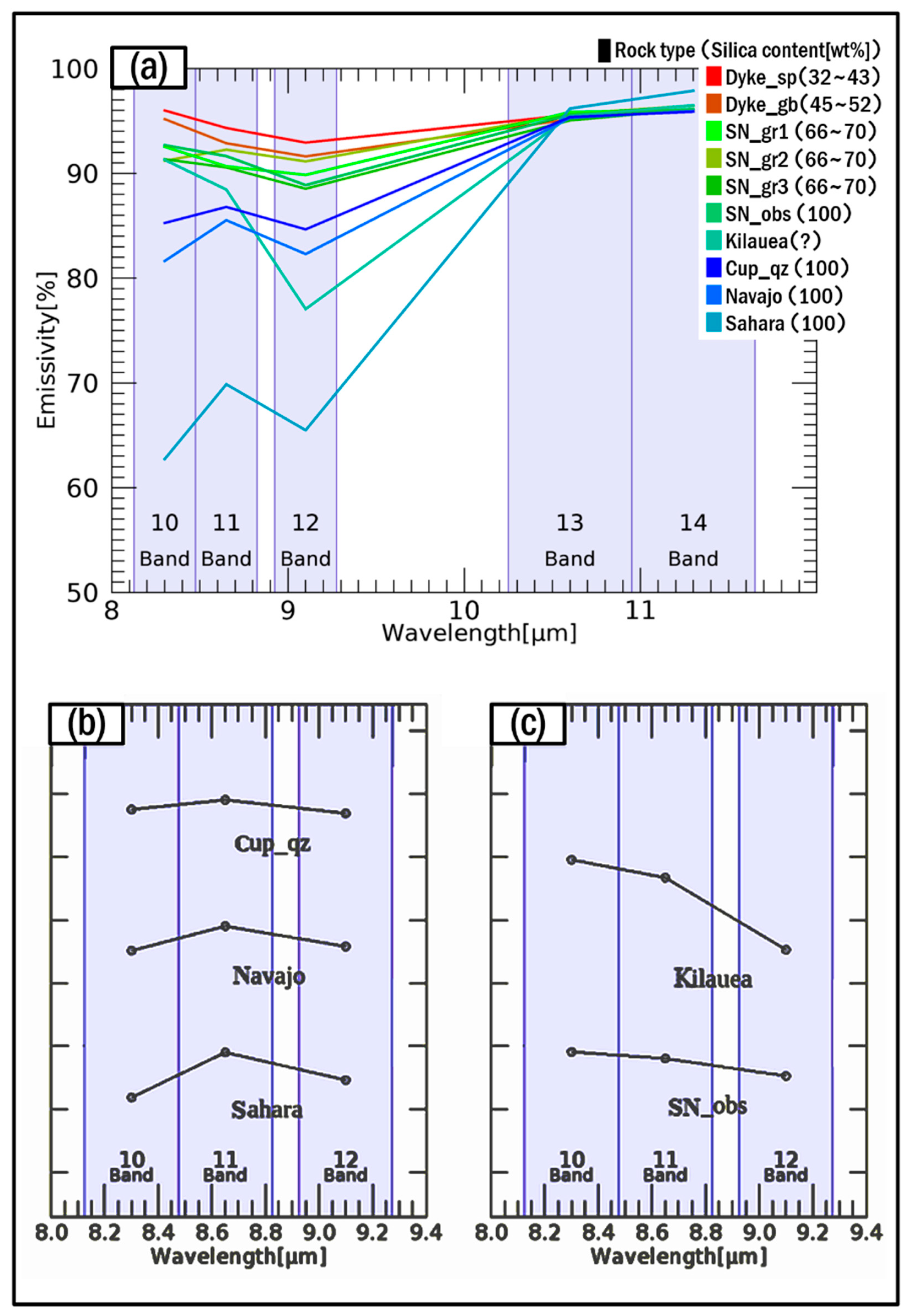
The emissivity patterns for rocks show a systematic relation to reflect the silica content and the types of mineral present [23]. Figure 1a shows the spectral shapes derived from ASTER TIR emissivity data at 10 locations around the world with distributions of different types of silicate rocks (Table 2). Several dozen pixels were sampled at each location and were averaged to represent the typical emissivity spectrum of each rock type. On the basis of the results in Figure 1a, new indices are proposed for silicate rocks: The T-depth, which represents the silica content, and the T-angle, which represents the mineral form. The T-depth represents a decrease in the emissivity in bands 10, 11, and 12, relative to those in bands 13 and 14, and it is defined as:
here B10, B11, B12, B13, and B14 are the emissivities of ASTER TIR bands 10, 11, 12, 13, and 14, respectively.
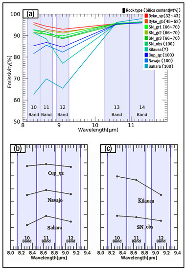
Figure 1.
(a) Typical emissivity spectra in the TIR region in the sampling areas; (b) typical emissivity spectra of bands 10, 11, and 12 in the three sampling areas, where quartzose materials are distributed; (c) typical emissivity spectra of SN_obs (obsidian) and Kilauea, where a thin amorphous silica layer covers the surface. Please note that the spectra in (b,c) are offset for clarity. The vertical scale resolution is 10% emissivity.
Table 2.
Characteristics of the sampling areas for thermal infrared (TIR) emissivity spectra.
The emissivities of felsic rocks with a higher silica content in bands 10, 11, and 12 are lower than those of mafic rocks (Figure 1a). Thus, felsic rocks have larger T-depths, and mafic rocks have smaller T-depths. A larger T-depth corresponds to a high silica content of the target rock. For example, the emissivity average of bands 10–12 was lowest for the quartzose sands in the Sahara Desert, followed by the Navajo Sandstone in Utah with almost 100% quartz grains; the basalt lava in Kilauea Volcano, Hawaii, with a thin silica coating [24]; and the quartzite in Cuprite, Nevada. The T-depth values of these targets were high, as shown in Table 3.
Table 3.
Average T-depth values in each sampling area.
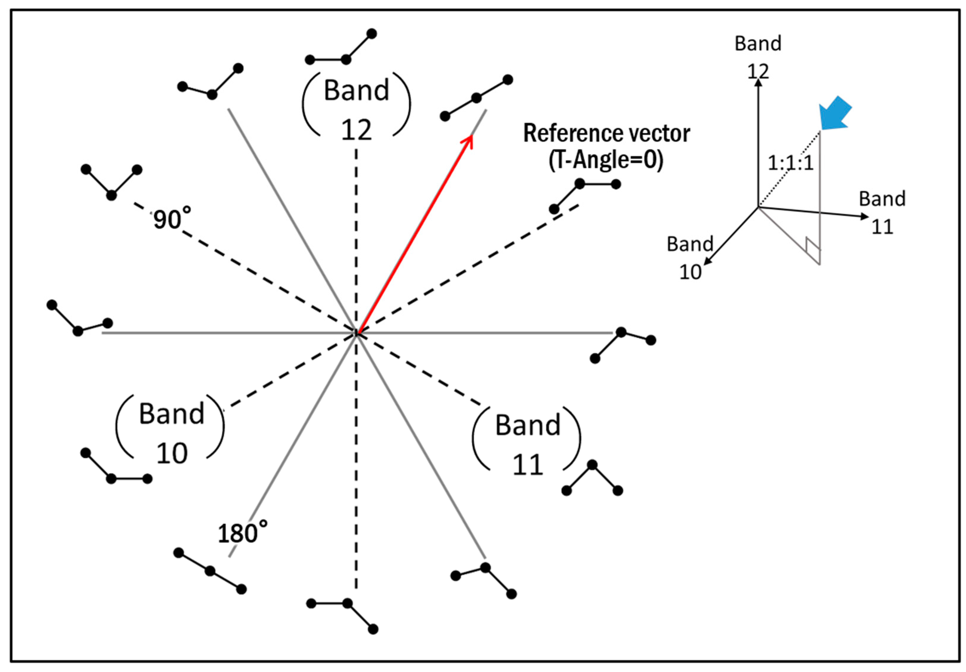
The T-angle quantifies the emissivity patterns in ASTER bands 10, 11, and 12 to detect the mineral form—in this particular case, quartz or amorphous silica—by using the orthogonal transformation. This index is defined as the angle between two vectors expressed in the three-dimensional space of the ASTER bands 10, 11, and 12 emissivities. The two vectors are a reference vector and a variable (or target) vector (Figure 2). In this case, the reference vector represents a spectral pattern linearly increasing from band 10 to 12 and is set to have an orientation of 0°. The transform coefficients were calculated according to the method by Jackson [25]. The T-angle is given by

Figure 2.
Concept of orthogonal transformation in the three-dimensional space of the reflectance of ASTER bands 10, 11, and 12.
The spectral patterns can be described by the T-angle, which ranges from 0° to 360°. Quartz-rich materials have a diagnostic spectral pattern in this wavelength region (Figure 1b), whereas amorphous-silica-rich materials have a different spectral pattern (Figure 1c), which is represented by T-angles of approximately 210° and 300°, respectively. Quartz has relatively low emissivity in ASTER bands 10 and 12, and a relatively high emissivity in band 11 due to its fundamental asymmetric Si-O-Si stretching vibration [17,23]. In contrast, amorphous-silica-rich materials such as glass, opal, and obsidian show emissivity patterns that decrease from band 10 to band 12 due to their broad emissivity depression at around 9.1 microns [24,26]. As the two proposed indices, T-depth and T-angle, have fixed value ranges, the index values derived from different scenes or different areas can easily be compared.
2.3.2. Delineating Carbonate Rocks
Carbonate rocks are generally detected using SWIR spectral data. However, in this study, a carbonate index for ASTER TIR data [17] was used to delineate carbonate rocks because ASTER SWIR band 9 data show some problems in the surface reflectance product. It may be possible to replace this index of 90 m spatial resolution with the relative band depth (RBD) of bands 7, 8, and 9 of 30 m spatial resolution when reliable surface reflectance data including SWIR band 9 are available. The carbonate index used here is defined as:
carbonate index = B13/B14.
2.3.3. Delineating Hydrothermal Alteration Zones
To map hydrothermal alteration areas, two clay mineral indices developed by Kurata and Yamaguchi [15] were adopted. The clay index quantifies the SWIR spectral patterns by using the orthogonal transformation, and the spectral pattern changes depending on type of clay mineral. This index is defined as the angle between two vectors expressed in the three-dimensional space of the reflectances of ASTER SWIR bands 5, 6, and 7 in a manner similar to the definition of the T-angle. The two vectors are a reference vector and a variable (or target) vector. The angle between the two vectors is calculated from the inner product of the vectors with elements representing the reflectances of ASTER SWIR bands 5, 6, and 7 and two orthogonal unit vectors. The transform coefficients were calculated according to the method by Jackson [25]. The clay index assigned to the H element is calculated using the following formula:
where B5, B6, and B7 are the reflectances of ASTER SWIR bands 5, 6, and 7, respectively. We used the ASTER standard data product of SWIR surface reflectance (AST_07XT), including the crosstalk correction. The spectral pattern of alunite takes a clay index of 10°, and the clay indices of kaolinite and montmorillonite would be approximately 45 and 90.
The index describing the clay mineral amount is defined as
This index indicates the depth of the absorption caused by the –OH radicals of clay minerals in the SWIR region corresponding to ASTER bands 5, 6, and 7.
SWIR depth = (B4 × 3)/(B5 + B6 + B7).
2.3.4. Allocation of Spectral Indices to the H and S Elements
The lithological indices were integrated by allocating each of them to the H or S element of the HSV color model. Figure 3 shows the meanings of the colors determined by the following procedure. In the integration stage, the following minerals were considered in order of descending priority: clay minerals, carbonate minerals, and silicate minerals. This order was selected because it reflects the general relative importance of these minerals in metal explorations. Namely, the indices of silicate rocks were first allocated to all pixels in the image as a background, then the carbonate and clay mineral indices were progressively overwritten to the pixels where these indices exceeded the corresponding threshold.

Figure 3.
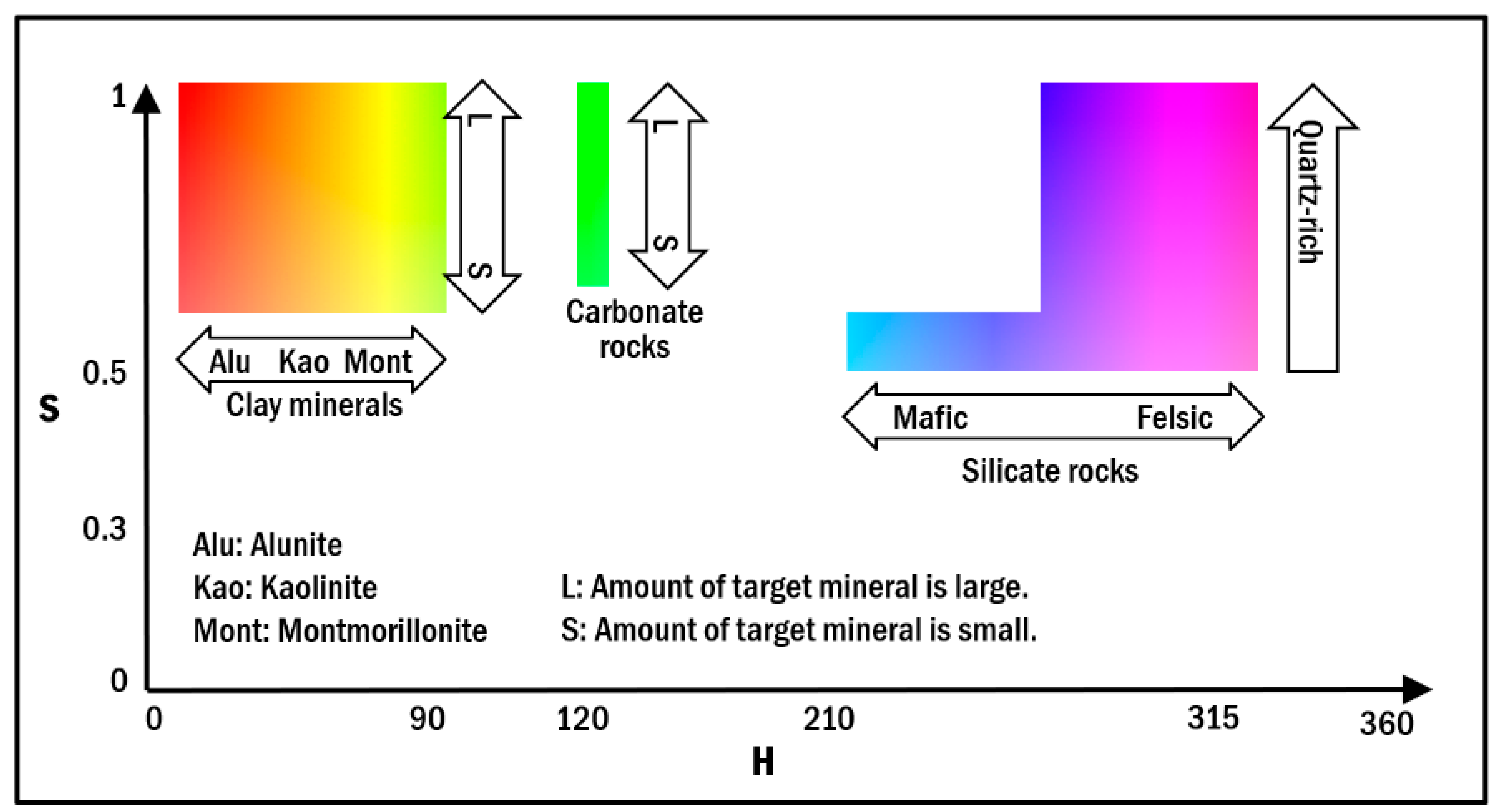
Meanings of the colors determined by the procedures to allocate lithological indices to the hue (H) and saturation (S) elements of the hue–saturation–value (HSV) color model.
The T-depth values ranging from 1.16 to 9.85 were linearly rescaled to the range 210–315 and assigned to the H element of the HSV color model; this means that the silica content is represented by the pixel color. The two thresholds 1.16 and 9.85 were determined empirically by comparing the T-depth values (Table 3) and rock types of target pixels on actual ASTER images. For example, the lower threshold of 1.16 corresponds to the average T-depth value of the mafic rocks that include the basalt in Cuprite and the mafic intrusions of the Great Dyke. Please note that the T-depth values in Table 3 are just typical examples. As we used approximately three times as many pixels to obtain the thresholds, the T-depth average in Table 3 does not coincide with the threshold. Pixels whose T-depth is lower than 1.16 are regarded as mafic rock and assigned an H value of 210°. Similarly, the higher threshold of 9.85 was determined using the T-depth values of the felsic rocks on actual ASTER images. Pixels whose T-depth is higher than 9.85 are regarded as felsic rock and assigned an H value of 300°. The thresholds for the clay and carbonate indices were similarly determined.
Silica-rich materials (e.g., quartzose sand and obsidian) are thus represented by H values close to 315, corresponding to pink, whereas silica-poor materials (e.g., basalt) are represented by H values close to 210, corresponding to blue. In this case, the S element was set to (0.5 + α), where α, which ranges from 0.0 to 0.5, was determined from the value of the T-angle, which represents the mineral form of the silicates, whether the target felsic rock is composed of crystalline quartz or amorphous silica. T-angles ranging from 210.0 to 310.0 were linearly rescaled to the given range of α values. This assignment means that the parts of the images in which the T-angle was between 210.0 and 310.0 are represented by a more vivid color for high T-angles, whereas other areas are displayed in a dull color. As a result of this process, quartz and amorphous silica could be distinguished from each other, as shown in Figure 4a–d, respectively.
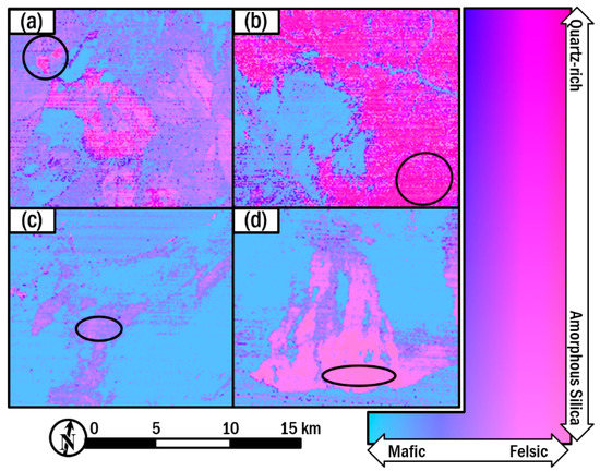
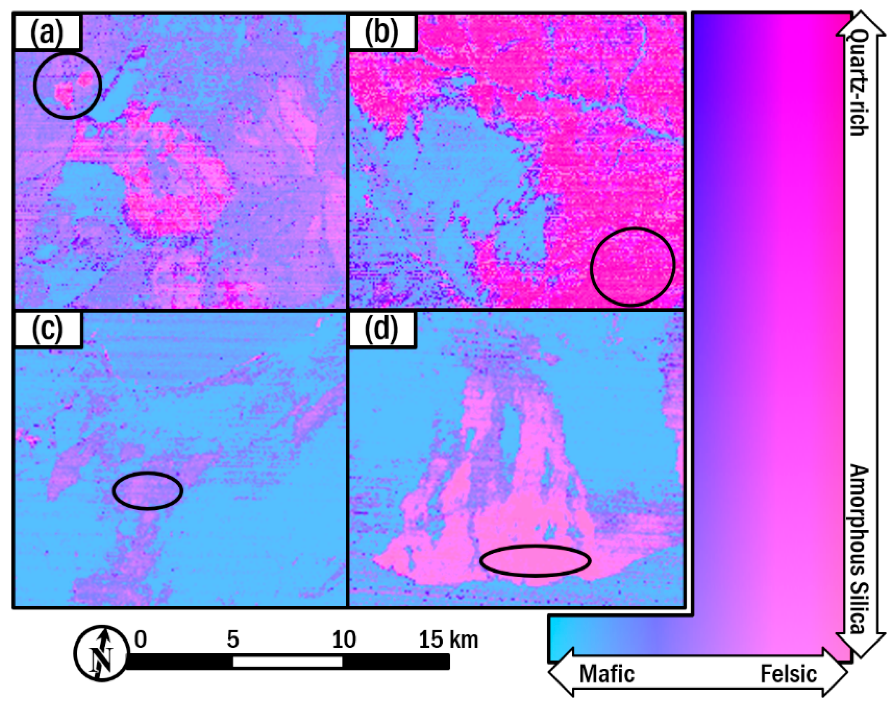
Figure 4.
Images generated by integrating the T-depth and T-angle, which can distinguish between quartz (a,b), and amorphous silica (c,d): (a) quartzite in Cuprite, Nevada, USA; (b) Navajo Sandstone in Utah, USA; (c) Obsidian in the hills in the southern part of Mono Lake, California, USA; (d) thin silica coating on pahoehoe lava in Kilauea, Hawaii, USA. The ellipses indicate representative areas where these target rocks are distributed. Coordinates of the ellipse centers; (a) 37°37′17.14″ N/117°17′26.87″ W, (b) 37°42′05.32″ N/111°22′35.22″ W, (c) 37°53′39.43″ N, 119°00′29.60″ W, (d) 19°16′34.93″ N, 155°09′21.74″ W.
Then, to integrate the carbonate index into the image, the carbonate index values were linearly rescaled to the range between 0.0 and 1.0 by excluding the top 2% and bottom 2% as unexpected values. This procedure is scene-dependent. In this case, pixels with rescaled indices exceeding the lower threshold of 0.65 were selected as areas with carbonate rocks. The H element of these pixels was then set to 120, corresponding to light green, and the S element was replaced by the rescaled index in the target area; this means that areas containing carbonate rocks are shown in light green with a vividness representing the index value.
Lastly, indices representing the clay mineral species (clay index) and amount (SWIR depth) were allocated to the H and S elements, respectively. For the purpose of visualizing gradual changes in the clay minerals in hydrothermal alteration zones, clay index values between 10.0 and 110.0, which includes the spectral patterns of alunite, kaolinite, and montmorillonite (or sericite)—minerals commonly distributed in hydrothermal alteration zones—were assigned to the H element after rescaling to the range of 0, corresponding to red, to 90, corresponding to greenish yellow, using the following formula:
where h is the clay index. The SWIR depth and carbonate index were rescaled to the range of 0.0 to 1.0 and were allocated to the S element. The pixels satisfying the following conditions were selected as hydrothermal alteration zones: (1) the clay index is between 10.0 and 110.0, and (2) the stretched SWIR-depth value exceeds 0.6. The H and S elements were modified for the pixels that fulfill these conditions.
2.4. DEM Visualization by the V Element
A new method of visualizing the topography as a grayscale relief map (GRM) obtained from DEM data was developed in this study. This method combines two existing methods: the overground openness by Yokoyama et al. [27] and the inverted slope by Yajima and Yamaguchi [28]. The overground openness describes a sky extent measured by a solid angle (steradian) over the point within a certain distance. In this particular case, it was measured at each pixel for an area within 30 m. The overground openness of a target pixel is defined as the average of the slope of the ground in eight radial directions, and the slope in each direction is determined by taking the maximum slope between the target pixel and the pixels within a certain distance in each direction. However, the actual topography cannot easily be understood from the overground openness because the angles of slopes are not shown, even though mountain ridges and valleys are accurately indicated. However, the inverted slope can be used to visualize the angles of slopes by using the Guth hybrid slope algorithm [29], which can estimate the slope at a target pixel by taking the maximum slope measured in eight radial directions from the target pixel to adjacent pixels. A steeper slope is expressed as darker in an inverted slope image, whereas a gentle slope is expressed as brighter; flat areas are expressed as white. As a result, characteristic topographical features (e.g., conus or tables) corresponding to different lithological units can be visually interpreted. However, both ridges and valleys are represented as white, and it is difficult to distinguish them in an inverted slope image, as shown in Figure 5a.

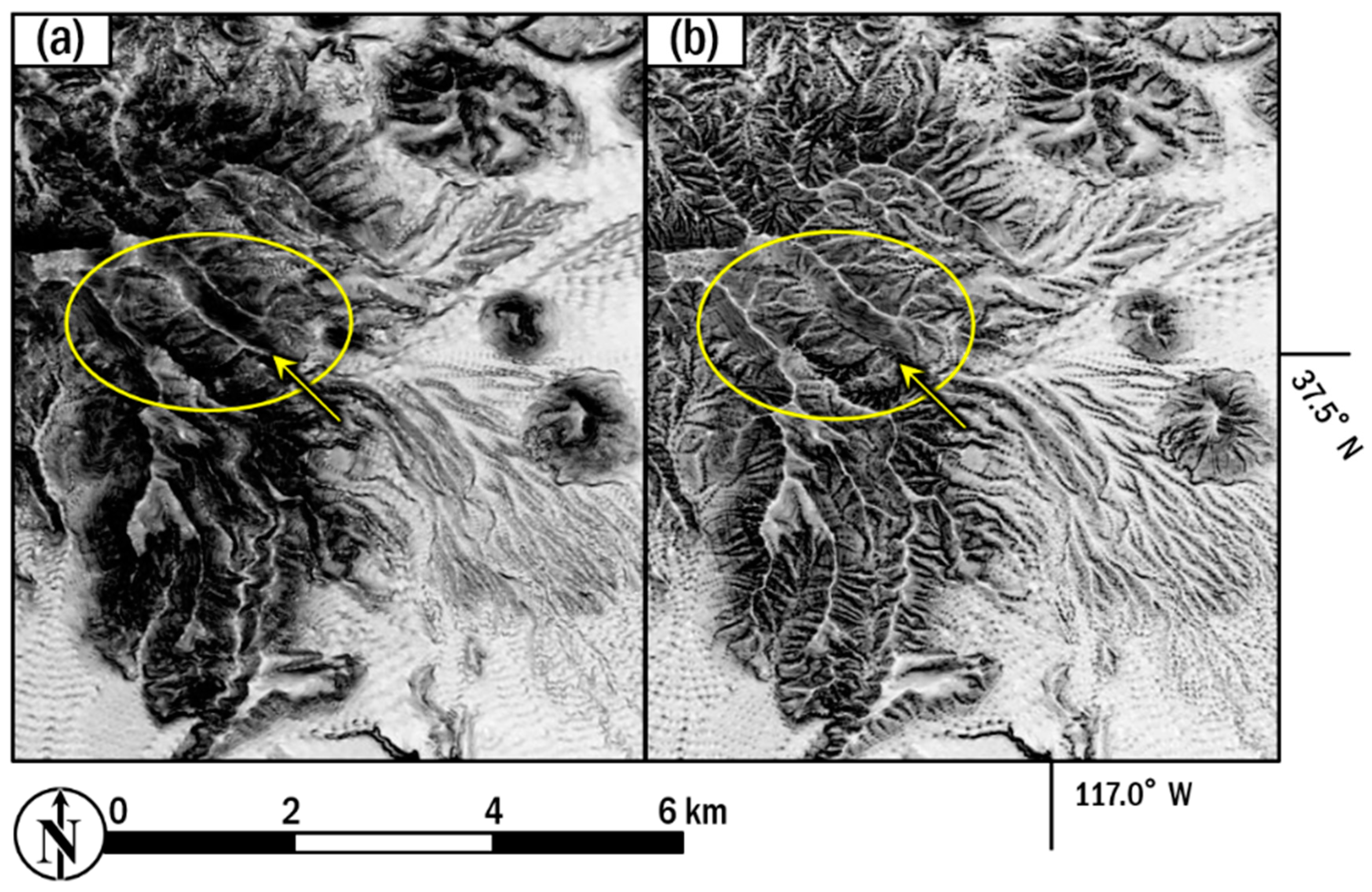
Figure 5.
(a) Inverted slope image of Stonewall Mountain located to the southeast of Cuprite; (b) Grayscale relief map (GRM) image of the same area. In (a), the valley trending northwest-southeast shown by the arrow is white and looks similar to the parallel white ridges in the ellipse. In (b), this valley is black and is easily distinguishable from the ridges in the ellipse.
The proposed GRM method utilizes the advantages of these two existing methods and combines them in the following equation:
In this study, the value of γ was set to 3.0 based on visual comparisons of images with several different values. The GRM is expressed in grayscale, and it can thus be allocated to the V element of the HSV color model. In addition, as this method is independent of the illumination direction, meaning there is no selective enhancement by illumination. Therefore, as shown in Figure 5b, mountain ridges (white) and valleys (black) are easily distinguishable in images generated using this new method.
3. Results
Figure 6 shows the results of applying the image processing method proposed in this study. All of the lithological indices and topographical information were combined to generate a single image that clearly exhibits the distribution of silicate rocks, carbonate rocks, and hydrothermal alteration zones, as well as the topography, using the HSV color model. The V elements, which correspond to the brightness of the colors, express the topography. Because dark colors indicate steep slopes, the topography is depicted as the surface ruggedness overlaid on the integrated image. Figure 7 shows GRM images along with photographs of the actual topographical features represented in the images.
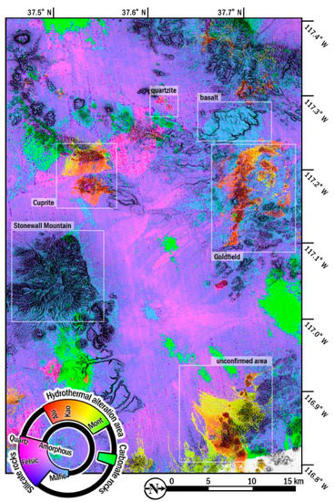
Figure 6.
Integrated image simultaneously exhibiting multiple lithological indices and the topography.
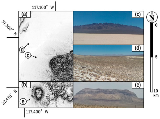
Figure 7.
GRM images and photographs the topographical features contained in the images: (a,b) GRM image; (c) Stonewall Mountains; (d) Alluvial plain; (e) Table plateau.
Colors ranging from blue to pink represent the silica content based on the T-depth. The silica content is low in blue areas as “basalt” in the image, high in pink areas, and intermediate when the color is between blue and pink. In addition, areas in which quartz is abundant on the surface are represented by vivid pink as “quartzite” in the image. Areas rich in carbonate rocks are shown in light green with a high vividness in the color image because the only carbonate rock area has higher carbonate index values than the other regions in the image. A hydrothermal alteration zone depicted in the integrated image exhibits a concentric pattern of hues; the color changes from red at the center to yellow and finally greenish yellow in the surrounding marginal areas. This characteristic pattern of colors indicates a typical spatial distribution of clay minerals in a hydrothermal alteration zone, from alunite in the central acidic alteration zone through kaolinite to montmorillonite in the peripheral alkali alteration zone (e.g., [20,30]). There are 3 zones having the characteristic pattern in the integrated image, Cuprite, Goldfield and an unconfirmed area.
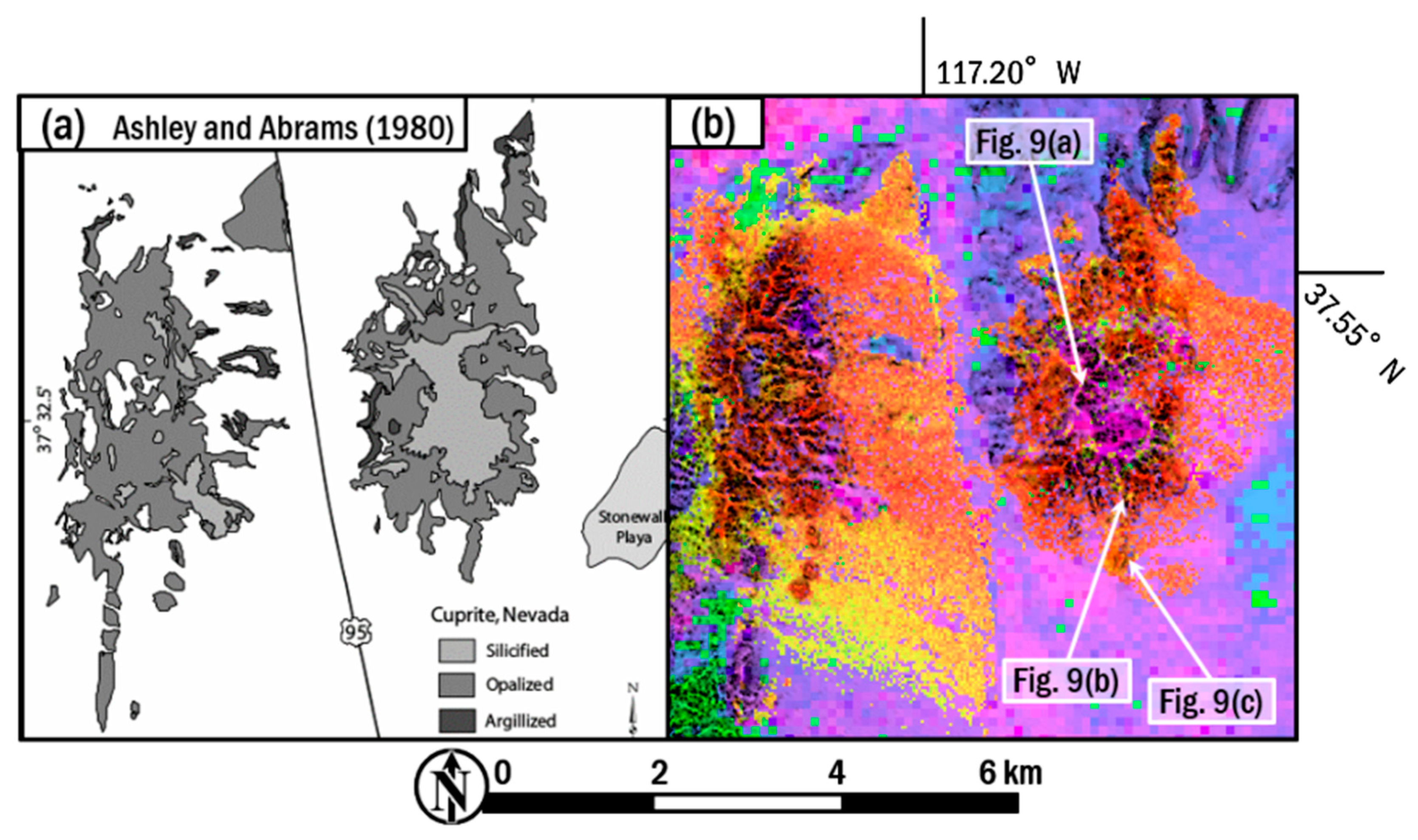
As shown in Section 2.3.4, it was confirmed that quartzite in Cuprite (Figure 4a), quartzose in Navajo Sandstone (Figure 4b), and obsidian near Mono Lake (Figure 4c) and amorphous silica on pahoehoe lava in Kilauea (Figure 4d) are displayed in a pinkish color because of their high T-depth values. Additionally, the former two, which consist of almost 100% quartz, are exhibited in a vivid color according to a particular T-angle value, whereas the latter two, which consists of amorphous silica, is exhibited in a pale color. A comparison of the present image with the results obtained in previous studies (e.g., [20,22]) reveals that chalcedony previously identified at the center of the eastern Cuprite hill (silicified area in Figure 8a) is clearly depicted in the image obtained using the proposed method, as shown in Figure 8b. In addition, a flat plateau of basalt in the southwestern part of the Goldfield area confirmed by Ashley [31] is also clearly depicted in pale blue, indicating mafic rock. Therefore, the T-depth can be considered to accurately represent the silica content of chemical compositions, and the T-angle can be used to successfully discriminate between quartz and amorphous silica, which have different mineralogical forms.
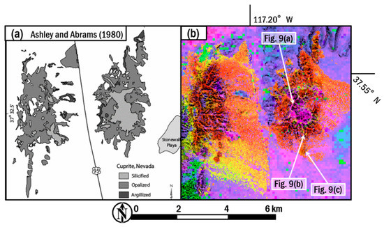
Figure 8.
Comparison between (a) Zonation of the hydrothermal alteration in Cuprite, Nevada by Ashley and Abrams [20] and (b) integrated image.
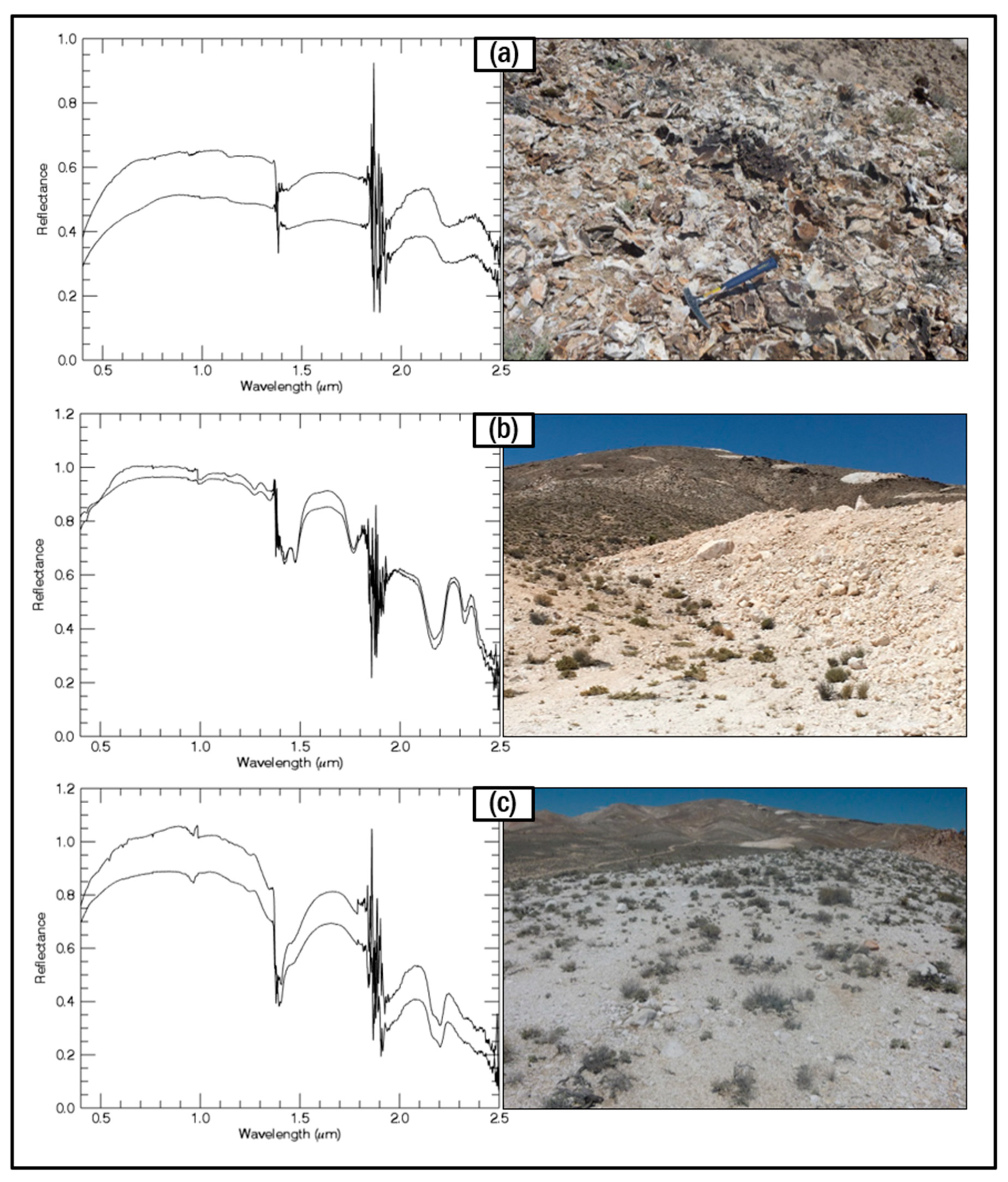
The results of the field verification are shown in Figure 9. The reflectance spectrum of the silicified rock with chalcedony at the center of the hill (Figure 9a) shows a weak absorption at 2.25 microns due to hydroxyl [32]. Alunite and kaolinite were identified in the hydrothermally altered rock samples collected south of the hill (Figure 9b,c). These results are consistent with the integrated image shown in Figure 8 as well as previous studies, indicating a typical zonation of hydrothermal alteration (e.g., [20]).

Figure 9.
Reflectance spectra and outcrop photographs of the hydrothermal alteration zone in Cuprite. See the locations in Figure 8. The upper and lower spectra for each sample indicate measurements for the fresh surface and the weathered surface, respectively. Absolute reflectance values are not meaningful due to imprecise measurement conditions. The noisy patterns at around 1.4 and 1.9 microns are due to the atmospheric water vapor as these spectra were obtained outdoor by using sunlight as an illumination source. (a) Silicified rock with chalcedony at the center of the alteration zone, (b) hydrothermally altered rock that includes alunite, and (c) hydrothermally altered rock that includes kaolinite.
The integrated image was also compared with the mineral map generated using the AVIRIS data [22]. Reddish areas in Figure 8b coincided well with the alunite areas, orange areas with the alunite + kaolinite or kaolinite areas, and yellowish areas with the kaolinite + white mica ± alunite or halloysite areas in Swayze et al. [22]. Calcite distributions in these two studies also agreed well.
4. Discussion
4.1. Integration Method
The method of integrating lithological and topological information in an HSV image was evaluated on the basis of two considerations: whether the HSV model is more appropriate than the conventional RGB color composite for data integration and whether the method shows site or target dependence. The RGB color composite has been widely used and explored; for example, it has been used to represent combinations of band ratios for various mineralogical features in [33]. An integrated image generated by the HSV color model (Figure 10a) and the corresponding RGB color composite image (Figure 10b) were compared based on how well the zonal structure of the hydrothermal alteration in the image could be visualized. The proposed integration method has several advantages over the conventional method. First, in the RGB color composite, up to three indices of the surface materials are directly allocated to the intensities of the RGB color primitives, whereas more than three appropriate indices can be arbitrarily selected for allocation to the HSV elements. Additionally, in the RGB color composite images, the mapping target must be assessed by interpreting the meanings of colors on a case-by-case basis, whereas the meanings of the colors in the HSV images generated with the proposed method are determined in advance, making them easily interpretable, and important targets can be readily enhanced by varying the S element value.

Figure 10.
Images showing the zonal structures of the hydrothermal alteration generated by: (a) The method proposed in this paper; (b) The RGB color composite method with the R, G, and B primitives representing the kaolinite group index, the AlOH group content, and the FeOH group content, respectively, as developed by Cudahy [34]. (c) Geological map of this area [35].
Regarding the second consideration, it is important to analyze different regions or targets because the proposed method may show site and/or target dependence. This study focused on the geological mapping of multiple types of rocks and minerals and selected a large target area (approximately 4,000 km2) containing distributions of a variety of rock types. Apart from the method having target dependence in that appropriate indices were selected for lithological mapping, there is additional site dependence in terms of the allocation of indices to HSV elements and rescaling them to a specific value range. The T-depth, T-angle, and clay index originally had definite value ranges, but the carbonate index and SWIR depth did not, and thus the resultant ranges could vary according to the data used in the analysis. This inconsistency forces the index range to be adjusted on a case-by-case basis, which causes site dependence. This means that the processes of allocating indices to the HSV elements is fundamentally dependent on both the target and the site, similarly to the problem of the RGB color composite technique.
However, the fundamental concept of this method can be applied to other targets and areas by selecting appropriate indices to detect the targets according to their spectral features. As a next step, it might be necessary to develop a method that can allocate index values to fixed ranges or select indices that have definite value ranges.
4.2. Lithological Indices and Geological Interpretation
As discussed, the integrated image could be used to easily interpret various geological situations that cannot be shown by separate lithological indices and topographical images. Some examples illustrating this are discussed here. First, the method for mapping hydrothermal alterations was successfully used to clearly visualize the different geological situations of the two hydrothermal alteration zones in Cuprite and Goldfield. Concentric zonation patterns were observed in both areas but with opposing patterns of changing colors: from red at the center of the concentric zonal structure to greenish yellow at the margin in Cuprite and from greenish yellow at the center to red at the margin in Goldfield. This implies that a region that underwent hydrothermal alteration with an acidic environment was distributed on the edge of the circular structure in Goldfield [31,36]. As highly acidic environments generally form at the center of hydrothermal alteration zones, this phenomenon could have produced a characteristic pattern in Goldfield in which the center of the hydrothermal alteration zone was not coincident with the center of the concentric zonal structure, unlike Cuprite, where the two centers were coincident. This inference is consistent with the suggestion in a previous study [31] that in Goldfield, a series of hydrothermal alteration zones is arranged in a circle along the circular structure formed by volcanic activity. This discussion indicates that this method could provide important geological information on hydrothermal alteration zones and the integrated image is a powerful tool to effectively and efficiently exhibit the geological characteristics.
Second, in the eastern part of Goldfield, the characteristic spatial distribution of the colors indicates the presence of a hydrothermal alteration zone (“unconfirmed area” in Figure 6). Clay minerals are distributed in the hills, and some linear distributions of greenish yellow and mixed distributions of red, yellow, and greenish yellow colors are observable in the flatlands around the hills. A geological interpretation of these patterns indicates that outcrops of a hydrothermal alteration zone are present on the hills and sediments derived from those outcrops were transported and spread onto the flat alluvial plains. This information was obtained from image interpretation only. Unfortunately access to the area is restricted due to military use. In a similar way, the topographical information enables the outcrops to be distinguished from the alluvia, which includes the sediments that flowed from the outcrops, as in the area around the flat plateau of basalt in the western part of Goldfield [35] (“basalt” in Figure 6). Furthermore, there are two different topographies in this area that were colored by vivid pink representing quartzose rocks but showed different morphologies: rugged and flat surfaces. These differences could have been caused by the different rock types, such as quartzite at the rugged hills and quartzose sedimentary rock or sediments in the flat surfaces. It can thus be concluded that the integrated image generated by the method proposed in this study is easily geologically interpretable.
Further studies are required to investigate the effects of vegetation cover. In this paper, we chose areas with sparse vegetation. It is likely that the H and S values for geological components will change if these components are mixed with a vegetation component. Removal of the vegetation component might be required prior to the application of the proposed integration method.
5. Conclusions
The goal of this study was to develop a new method of combining and visualizing multiple lithological indices derived from ASTER data in different wavelength regions and topography derived from DEM data in a single-color image that can be easily interpreted from a geological point of view. The proposed method consists of three parts: a technique to combine multiple indices using the HSV color model, the derivation of appropriate spectral indices to discriminate among different lithologies, and a method of visualizing the topography derived from DEM data. Consequently, a method that can be used to visualize geological information was successfully developed, and the resulting images were demonstrated to be more easily interpretable than those generated using conventional methods. It was confirmed that integrated images generated by combining lithological indices and topographical information enable the interpretation of detailed geological situations. The integration method can also be applied to various targets by adjusting the spectral indices and their allocation to the elements in the HSV color model. The newly developed lithological indices, the T-depth and T-angle, have definite value ranges and thus enable scene-independent analysis of silicate rocks, although the new method still has some shortcomings and target dependence. For example, the quantitative correspondence between the index values of T-depth and silica content of the actual lithology is not clear. Furthermore, the parameters used in the allocation process of the carbonate index and SWIR depth as well as the ranges of index values and thresholds are site-dependent. These points must be improved when the method is applied to other regions or geological targets. Regarding the visualization of the topography, it was confirmed that the new GRM method can clearly exhibit topographical differences.
The integration of multiple indices was effective in the geological mapping performed in this study. By adopting the proposed method of integrating multiple indices, even people who are not familiar with remote sensing can use geological remote sensing more easily to detect or map a particular geological unit and better understand its characteristics. This would facilitate the introduction of geologic remote sensing to geological studies and would contribute to bridging the gap between the fields of geology and geological remote sensing.
Author Contributions
Conceptualization, methodology, field validation and writing, K.K. and Y.Y.; programming and data curation, K.K.; funding acquisition, Y.Y.
Funding
This work was funded by JSPS KAKENHI (Grant no. 15H04225).
Acknowledgments
We would like to thank NASA and LPDAAC for providing the ASTER data used in this study, and USGS for providing the 3DEP DEM dataset used in this study.
Conflicts of Interest
The authors declare no conflict of interest.
References
- Van der Meer, F.D.; van der Werff, H.M.A.; van Ruitenbeek, F.J.A.; Hecker, C.A.; Bakker, W.H.; Noomen, M.F.; van der Meijde, M.; Carranza, E.J.M.; Smeth, J.B.D.; Woldai, T. Multi- and hyperspectral geologic remote sensing: A review. Int. J. Appl. Earth Obs. Geoinf. 2012, 14, 112–128. [Google Scholar] [CrossRef]
- Kereszturi, G.; Schaefer, L.N.; Schleiffarth, W.K.; Procter, J.; Pullanagari, R.R.; Mead, S.; Kennedy, B. Integrating airborne hyperspectral imagery and LiDAR for volcano mapping and monitoring through image classification. Int. J. Appl. Earth Obs. Geoinf. 2018, 73, 323–339. [Google Scholar] [CrossRef]
- Rogge, D.; Rivard, B.; Segl, K.; Grant, B.; Feng, J. Mapping of NiCu–PGE ore hosting ultramafic rocks using airborne and simulated EnMAP hyperspectral imagery, Nunavik, Canada. Remote Sens. Environ. 2014, 152, 302–317. [Google Scholar] [CrossRef]
- Kruse, F.A. Mapping surface mineralogy using imaging spectrometry. Geomorphology 2012, 137, 41–56. [Google Scholar] [CrossRef]
- Yamaguchi, Y.; Kahle, A.B.; Tsu, H.; Kawakami, T.; Pniel, M. Overview of Advanced Spaceborne Thermal Emission and Reflection Radiometer (ASTER). IEEE Trans. Geosci. Remote Sens. 1998, 36, 1062–1071. [Google Scholar] [CrossRef]
- Rowan, L.C.; Wetlaufer, P.H.; Goetz, A.F.H.; Billingsley, F.C.; Stewart, J.H. Discrimination of Rock Types and Detection of Hydrothermally Altered Areas in South-Central Nevada by the Use of Computer-Enhanced ERTS Images; Geological Survey Professional Paper; U.S. Department of Energy Office of Scientific and Technical Information: Oak Ridge, TN, USA, 1976; Volume 883, p. 35.
- Kruse, F.A.; Lefkoff, A.B.; Boardman, J.W.; Heidebrecht, K.B.; Shapiro, A.T.; Barloon, P.J.; Goetz, A.F.H. The spectral image-processing system (SIPS)—Interactive visualization and analysis of imaging spectrometer data. Remote Sens. Environ. 1993, 44, 145–163. [Google Scholar] [CrossRef]
- Yamaguchi, Y.; Naito, C. Spectral indices for lithologic discrimination and mapping by using the ASTER SWIR bands. Int. J. Remote Sens. 2003, 24, 4311–4323. [Google Scholar] [CrossRef]
- Fatima, K.; Khattak, M.U.K.; Kausar, A.B.; Toqeer, M.; Haider, N.; Rehman, A.U. Minerals identification and mapping using ASTER satellite image. J. Appl. Remote Sens. 2017, 11, 46006. [Google Scholar] [CrossRef]
- Jakob, S.; Gloaguen, R.; Laukamp, C. Remote sensing-based exploration of structurally-related mineralizations around Mount Isa, Queensland, Australia. Remote Sens. 2016, 8, 358. [Google Scholar] [CrossRef]
- Zimmermann, R.; Brandmeier, M.; Andreani, L.; Mhopjeni, K.; Gloaguen, R. Remote sensing exploration of Nb-Ta-LREE-enriched carbonatite (Epembe/Namibia). Remote Sens. 2016, 8, 620. [Google Scholar] [CrossRef]
- Fujisada, H.; Urai, M.; Iwasaki, A. Technical methodology for ASTER global DEM. IEEE Trans. Geosci. Remote Sens. 2012, 50, 3725–3736. [Google Scholar] [CrossRef]
- Takaku, I.; Tadono, T.; Tsutsui, K. Generation of high resolution global DSM from ALOS PRISM. Int. Arch. Photogramm. Remote Sens. Spat. Inf. Sci. 2014, XL-4, 243–248. [Google Scholar] [CrossRef]
- Whelley, P.L.; Glaze, L.S.; Calder, E.S.; Harding, D.J. LiDAR-derived surface roughness texture mapping: Application to Mount St. Helens pumice plain deposit analysis. IEEE Trans. Geosci. Remote Sens. 2014, 52, 426–438. [Google Scholar] [CrossRef]
- Kurata, K.; Yamaguchi, Y. Combining multiple lithological indices derived from ASTER data by using the HSV color model. J. Remote Sens. Soc. Jpn. 2018, 38, 163–173, (In Japanese with an English abstract). [Google Scholar]
- Smith, R.A. Color gamut transform pairs. ACM Siggraph Computer Graphics 1978, 3, 12–19. [Google Scholar] [CrossRef]
- Ninomiya, Y.; Fu, B. Quartz index, carbonate index and SiO2 content index defined for ASTER TIR data. J. Remote Sens. Soc. Jpn. 2002, 22, 50–61, (In Japanese with an English abstract). [Google Scholar]
- Gillespie, A.R.; Matsunaga, T.; Rokugawa, S.; Hook, S.J. Temperature and emissivity from Advanced Thermal Emission and Reflection Radiometer (ASTER) images. IEEE Trans. Geosci. Remote Sens. 1998, 36, 1113–1126. [Google Scholar] [CrossRef]
- Abrams, M.J.; Ashley, R.P.; Rowan, L.C.; Goetz, A.F.H.; Kahle, A.B. Mapping of hydrothermal alteration in the Cuprite mining district, Nevada using aircraft scanner images for the spectral region 0.46–2.36 μm. Geology 1977, 5, 713–718. [Google Scholar] [CrossRef]
- Ashley, R.P.; Abrams, M.J. Alteration Mapping Using Multispectral Images-Cuprite Mining District, Esmeralda County, Nevada; U.S. Geological Survey Open File Report; U.S. Geological Survey: Reston, VA, USA, 1980; pp. 80–367.
- Kahle, A.B.; Goetz, A.F.H. Mineralogic information from a new airborne thermal infrared multispectral scanner. Science 1983, 222, 24–27. [Google Scholar] [CrossRef]
- Swayze, G.A.; Clark, R.N.; Goetz, A.F.H.; Livo, K.E.; Breit, G.N.; Kruse, F.A.; Sutley, S.J.; Snee, L.W.; Lowers, H.A.; Post, J.L. Mapping advanced argillic alteration at Cuprite, Nevada using imaging spectroscopy. Econ. Geol. 2014, 109, 1179–1221. [Google Scholar] [CrossRef]
- Lyon, R.J.P. Analysis of rocks by spectral infrared emission (8 to 25 microns). Econ. Geol. 1965, 60, 715–736. [Google Scholar] [CrossRef]
- Kahle, A.B.; Gillespie, A.R.; Abbott, E.A.; Abrams, M.J.; Walter, R.E.; Hoover, G. Relative dating of Hawaiian lava flows using multispectral thermal infrared images: A new tool for geologic mapping of young volcanic terranes. J. Geophys. Res. 1988, 93, 15239–15251. [Google Scholar] [CrossRef]
- Jackson, R.D. Spectral indices in n-space. Remote Sens. Environ. 1983, 13, 409–421. [Google Scholar] [CrossRef]
- Balick, L.; Gillespie, A.; French, A.; Danilina, I.; Allard, J.-P.; Mushkin, A. Longwave thermal infrared spectral variability in individual rocks. IEEE Geosci. Remote Sens. Lett. 2009, 6, 52–56. [Google Scholar] [CrossRef]
- Yokoyama, R.; Shirasawa, M.; Kikuchi, Y. Representation of topographical features by openness. J. Jpn. Soc. Photogramm. Remote Sens. 1999, 38, 26–34, (In Japanese with an English abstract). [Google Scholar]
- Yajima, T.; Yamaguchi, Y. Application of inverted slope images generated from ASTER GDEM to geological mapping. In Proceedings of the 56th Spring Conference of the Remote Sensing Society of Japan, Ibaraki, Japan, 15–16 May 2014; pp. 57–58, (In Japanese with an English abstract). [Google Scholar]
- Guth, P.L. Slope and aspect calculations on gridded digital elevation models: Examples from a geomorphometric toolbox for personal computers. Z. Geomorphol. Suppl. 1995, 101, 31–52. [Google Scholar]
- Bedini, E.; van der Meer, F.; van Ruitenbeek, F. Use of HyMap imaging spectrometer data to map mineralogy in the Rodalquilar caldera, southeast Spain. Int. J. Remote Sens. 2009, 30, 327–348. [Google Scholar] [CrossRef]
- Ashley, R.P. Relation between Volcanism and Ore Deposition at Goldfield, Nevada; Nevada Bureau of Mines and Geology Report; Nevada Bureau of Mines and Geology: Reno, NV, USA, 1979; Volume 33, pp. 77–86. [Google Scholar]
- Hunt, G.R.; Salisbury, J.W.; Lenhoff, C.J. Visible and near-infrared spectra of minerals and rocks: VII. Acidic igneous rocks. Mod. Geol. 1973, 4, 217–224. [Google Scholar]
- Kalinowski, A.A.; Oliver, S. ASTER Processing Manual. Remote Sensing Applications; Internal Report; Geoscience Australia: Canberra, Australia, 2004. [Google Scholar]
- Cudahy, T. Australian Satellite ASTER Geoscience Product Notes, Version 1; No. EP-30-07-12-44; CSIRO ePublish: Canberra, Australia, 2012. [Google Scholar]
- Albers, P.J.; Stewart, H.J. Geology and Mineral Deposits of Esmeralda County, Nevada; Nevada Bureau of Mines and Geology: Reno, NV, USA, 1972; Volume 78, p. 88. [Google Scholar]
- Blakely, R.J.; John, D.A.; Box, S.; Berger, B.R.; Fleck, R.J.; Ashley, R.P.; Newport, G.R.; Heinemeyer, G.R. Crustal controls on magmatic-hydrothermal systems: A geophysical comparison of White River, Washington, with Goldfield, Nevada. Geosphere 2007, 3, 91–107. [Google Scholar] [CrossRef]


© 2019 by the authors. Licensee MDPI, Basel, Switzerland. This article is an open access article distributed under the terms and conditions of the Creative Commons Attribution (CC BY) license (http://creativecommons.org/licenses/by/4.0/).