An Efficient Framework for Remote Sensing Parallel Processing: Integrating the Artificial Bee Colony Algorithm and Multiagent Technology

Abstract

Remote sensing (RS) image processing can be converted to an optimization problem, which can then be solved by swarm intelligence algorithms, such as the artificial bee colony (ABC) algorithm, to improve the accuracy of the results. However, such optimization algorithms often result in a heavy computational burden. To realize the intrinsic parallel computing ability of ABC to address the computational challenges of RS optimization, an improved multiagent (MA)-based ABC framework with a reduced communication cost among agents is proposed by utilizing MA technology. Two types of agents, massive bee agents and one administration agent, located in multiple computing nodes are designed. Based on the communication and cooperation among agents, RS optimization computing is realized in a distributed and concurrent manner. Using hyperspectral RS clustering and endmember extraction as case studies, experimental results indicate that the proposed MA-based ABC approach can effectively improve the computing efficiency while maintaining optimization accuracy.

1. Introduction

Image processing is of great importance for remote sensing (RS) applications [1], such as classification [2], clustering [3,4,5], and endmember extraction [6,7]. Recently, many RS image processing problems have been converted to optimization problems to improve the results’ accuracy [8,9]. For example, an RS clustering problem can be converted to an optimization problem that minimizes the distance between the pixel and the cluster center [10] and an RS endmember extraction problem to a problem that minimizes the remixed error [11,12]. Because these RS optimization problems are nonlinear and are difficult to solve using traditional linear approaches, the artificial bee colony (ABC) algorithm, an outstanding swarm intelligence (SI) algorithm, has been widely used for its ability to address nonlinear problems [5,13,14,15,16]. Experiments have demonstrated the improved results achieved by utilizing this intelligent algorithm.

However, using ABC to solve RS optimization problems is a computationally expensive task [17,18] because ABC is an iterative-based stochastic search algorithm that is usually executed sequentially in a central processing unit (CPU). In each iteration, each bee in the population must execute time-consuming operations, such as RS optimization’s fitness evaluation, to obtain new solutions [18]. Therefore, as these operations’ complexity and the RS image volume increase, the computational burden increases substantially, resulting in poor performance.

To contend with the aforementioned computational challenges, efforts have been made to establish parallel computing approaches. The technique of employing graphics processing units (GPUs) is a widely used approach [6,19,20,21]. A GPU has a massively parallel architecture consisting of thousands of small arithmetic logic units (ALUs), which are efficient for handling computing-intensive tasks simultaneously [22]. With GPU-based RS optimization, the data processing behaviors of each individual in SI algorithms that contain large volumes of calculations, especially the most computationally intensive fitness evaluation, are offloaded onto the GPUs’ threads for parallel computation [6,18]. During such parallel computation, an RS image is usually divided into many subimages, and multiple threads execute the same computation on different RS subimages in parallel. However, since in a bee swarm each individual’s behavior is operated on an entire RS image, after multiplying the number of subimages by the number of individuals, the number is often greater than the number of threads that the GPU hardware can provide; as a result, it is hard to implement multiple individuals’ calculation behavior in parallel.

To efficiently achieve parallel execution of individuals’ behavior, a multiagent (MA)-based ABC approach for RS optimization was proposed by utilizing distributed parallel computing based on the CPU [17]. This approach treats food sources and bees in ABC as different agents, which are distributed and concurrently behave in multiple processor units (computers or hosts). By communicating through the network, different agents interact with each other to obtain an optimal solution, thus significantly increasing the computation efficiency. However, the agents’ behaviors designed in [17] are relatively redundant, resulting in increased communication costs for its dispersed agents’ behaviors, which is further analyzed in Section 3.

To further increase the computational efficiency of RS optimization while using the ABC algorithm, this paper proposes an improved MA-based ABC approach by appropriately integrating agents’ behaviors to reduce communication among agents. The effectiveness and efficiency of the new method are demonstrated based on RS image clustering [5] and endmember extraction [16]. The remainder of this paper is organized as follows. Section 2 presents relevant theory pertaining to remote sensing optimization, the ABC algorithm, and multiagent system technology. Then, the basic concept of the improved MA-based ABC approach and the framework design are described in detail in Section 3. Section 4 introduces two RS optimization tasks as case studies, clustering and endmember extraction. The corresponding experiments and results are presented in Section 5 and Section 6. Finally, a discussion and a conclusion are provided in Section 7 and Section 8.

2. Theory

2.1. Remote Sensing Optimization

Many RS-related problems, such as clustering, endmember extraction, and target detection, essentially involve maximizing or minimizing results on certain indexes by computation. For example, for clustering, researchers usually try to minimize the distance among points within a cluster or maximize the distance among multiple classes. In addition, endmember extraction requires maximizing the spectral angle, maximizing the internal maximum volume, or minimizing the external minimum volume of points in spectral spaces. By treating these indexes as objective functions, these problems can be abstracted as optimization problems and expressed as follows:

$$\begin{array}{l}\min /\max f(x)\\ \mathrm{st}.x\in \Omega \end{array}$$

(1)

where $f(x)$ is the objective function of an optimization problem, $x$ is a solution, and $\Omega$ represents the constraints that the solution must satisfy.

2.2. The ABC Algorithm

The ABC algorithm [23] is a method for finding an optimal solution to an optimization problem by simulating the foraging behavior of a bee colony in nature. In the ABC algorithm, each scout bee randomly generates a feasible solution (food source) initially. Then, employed bees search around their corresponding food sources (feasible solutions) to generate new solutions with the participation of randomly selected neighborhood solutions. Once all of the food sources are updated with those with better fitness values, each onlooker bee pseudorandomly selects a food source (a feasible solution), searches around it to generate a new solution, and updates the food source with the better solution. If a food source is not updated for a long time, it will be abandoned, and a new food source will be obtained by a scout bee’s random selection. The bees’ behaviors will be iterated until an optimal solution is found. The entire procedure is depicted in Figure 1.

2.3. Multiagent System

An agent is a software component that has autonomy in providing an interoperable interface for a system [24]. The use of a multiagent system (MAS) is a technique for modeling complex problems. An MAS is constructed by multiple autonomous agents that interact with each other directly by communication and negotiation or indirectly by influencing the environment to fulfill local and global tasks [24,25,26]. Combining an MAS with swarm intelligence algorithms, such as ABC, in a distributed and parallel manner can be effective to shorten the computational time of a complex optimization problem [27]. Usually, the individuals in swarm intelligence algorithms can be treated as a series of heterogeneous agents in an MAS involving different computing processors with diverse goals, constraints, and behaviors. By collaborating among these agents, the optimal solution can be achieved in a distributed manner. For example, in [17], each artificial bee and food source are implemented as independent software agents who run separately and simultaneously in an MAS, with an administration agent controlling the flow work of the RS clustering algorithm. One major advantage of such an MAS is a reduction in computational time because the computational burdens are offloaded onto different processors. Furthermore, the failure of one agent will not disturb the entire algorithm’s calculat9ion, which is helpful for ensuring the robustness of the optimization framework.

3. Framework Design

The design of the improved MA-based ABC framework mainly consists of three parts: agents’ role design, communication design, and behavior design. This section first elaborates the design of each part and then compares this improved framework with the former framework proposed in [17].

3.1. Agents’ Role Design

Two types of agent roles are designed in this framework, massive bee agents and one administration agent. These agents are located in different computing nodes within the same network through which they can communicate with each other via messages. The agents’ role design is depicted in Figure 2.

In [17], bee agents are only responsible for a neighborhood search to generate new solutions in the employed and onlooker bee phase, which introduces an extra communication cost, as indicated in Section 2. In this paper, we redesign the bee agent with the potential to decrease the frequency of communication. In addition to a neighborhood search, each bee agent has more tasks to be executed to maintain its corresponding solution, which include (1) generating a random solution in the initial phase and the scout bee phase, (2) evaluating the solutions’ fitness, (3) updating the maintenance solution, and (4) recording the number $N_{\mathrm{limit}}$, which indicates that a solution has not been updated, to control the initiation and termination of the scout bee phase. These four behaviors are assigned to food source agents in [17].

Similarly to [17], the administration agent is responsible for the overall control of the algorithm, which includes the following functions: (1) exerting control over agents’ lifecycle, namely, generating new bee agents in different computing nodes during the initial stage and killing them at the end of the algorithm; (2) executing data initialization; (3) determining the solutions participating in the neighborhood search; (4) performing iteration and convergence control; and (5) recording and outputting the optimal solution.

3.2. Agents’ Communication Design

In this paper, a message-passing mechanism is adopted for the smooth implementation of the algorithm. All agents communicate with each other through the network by messages. According to the standard of agent communication language (ACL), each message contains at least five fields: the sender, the receivers, contents, language, and a communicative act [24].

For example, in ABC’s employed bee phase, the administrator agent will pass a neighborhood solution to each bee agent before executing the neighborhood search. Therefore, the sender of the message is the administrator agent, and the receiver is a bee agent. The message content contains the neighborhood solution, which is coded in the language of Java by serialization in our design. Under these circumstances, the sender (the administrator agent) wants the receiver (a bee agent) to perform an action (begin its neighborhood search); thus, the communicative act should be set as REQUEST. However, in certain other situations, the sender only wants the receiver to be aware of a fact, such as a bee agent notifying the administrator agent while completing a scout bee behavior; thus, the communicative act should be set as INFORM.

3.3. Agents’ Behavior Design

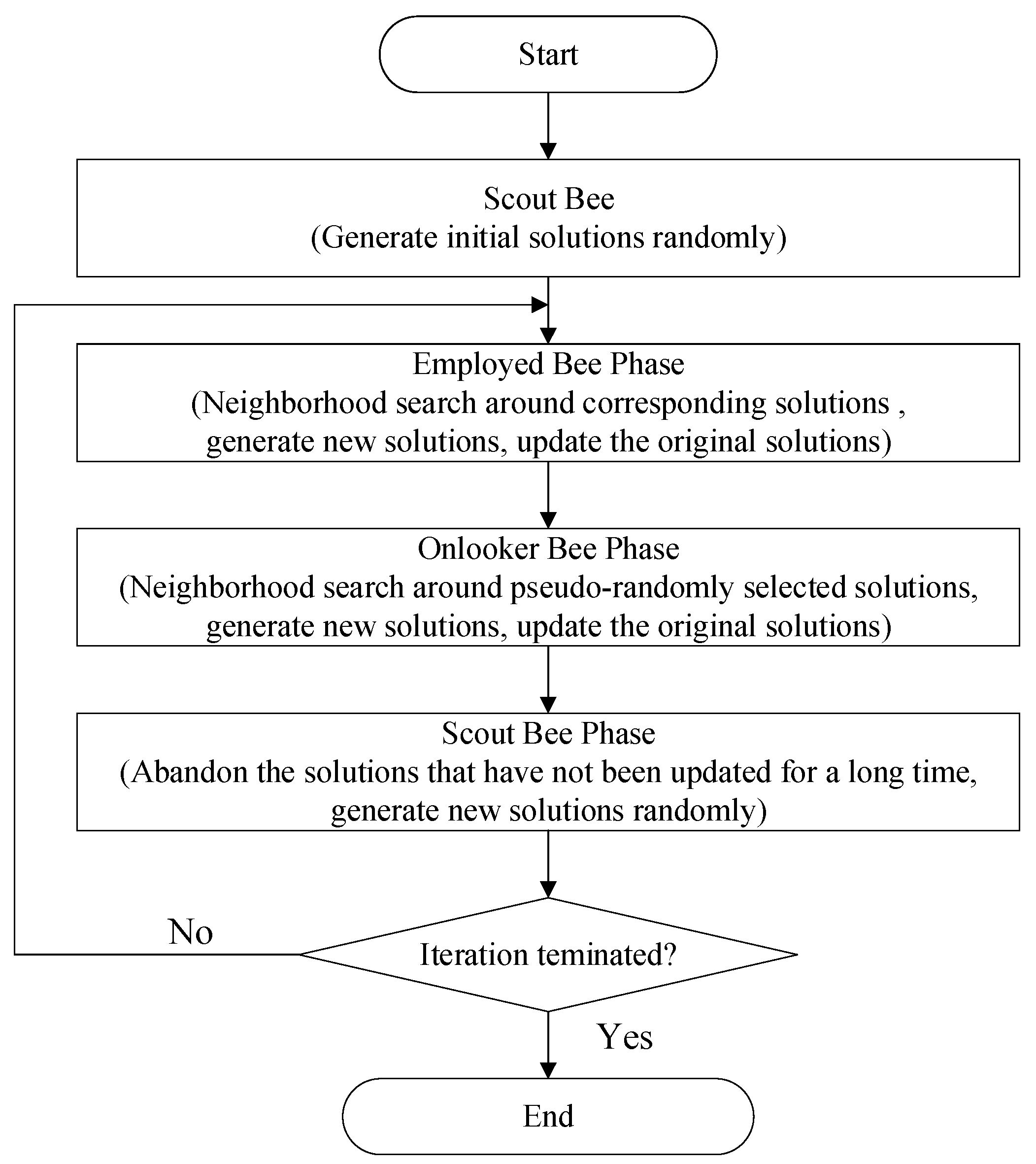
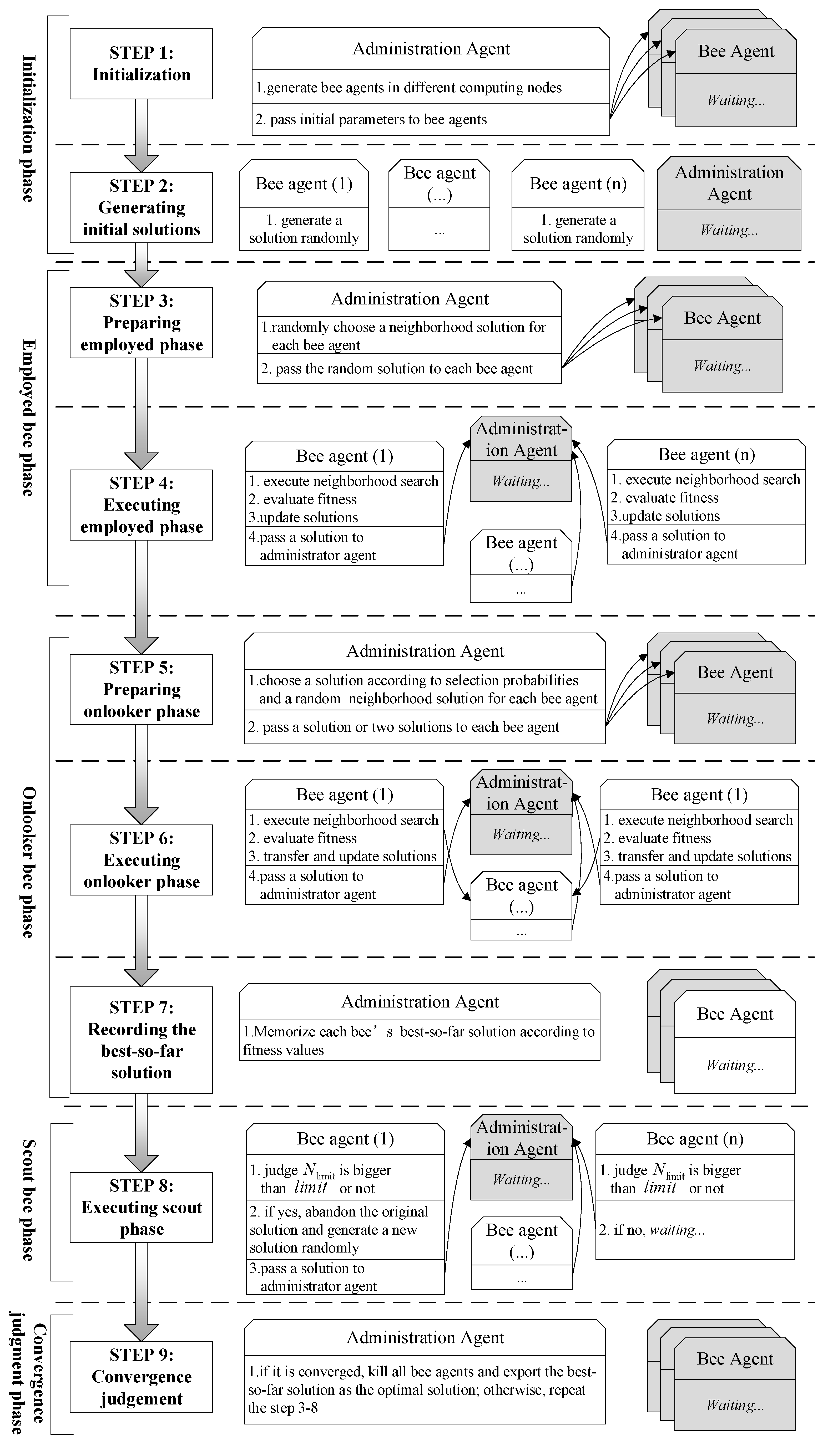
The agents’ behavior in an MA framework is tightly coupled with the procedure of the ABC algorithm. There are five phases in ABC: the initial phase, the employed bee phase, the onlooker bee phase, the scout bee phase, and the convergence judgment phase (Figure 3).

(1) Initialization phase

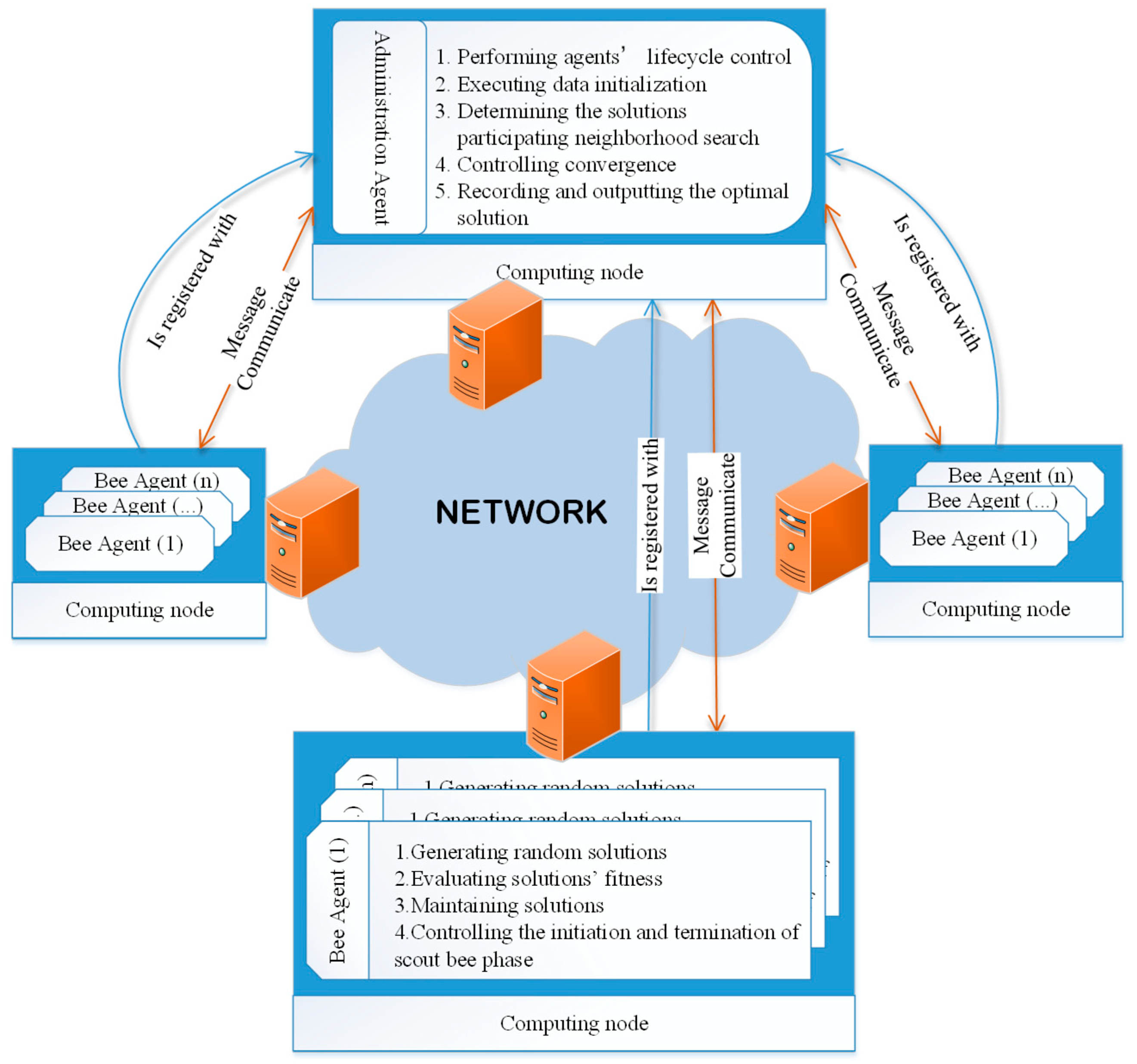
First, we launch an administration agent and set initial parameters, including MA-related data, such as the number of bee agents, the network address list of computing nodes that can participate in the parallel computation, and RS-optimization-related initial data, such as the number of clustering centers in the problem of hyperspectral image clustering.

Then, the administration agent will generate multiple bee agents in different computing nodes according to the parameters of the network address list and pass the RS-optimization-related initial parameters to each bee agent.

After receiving the initial parameters, each bee agent will generate a random solution.

(2) Employed bee phase

First, the administration agent will pass to each bee agent a random neighborhood solution through the network. Then, the $k^{th}$ bee agent maintaining solution $X_k=\{x_{k,1},x_{k,2},\cdots x_{k,m\times L}\}$ with fitness $fi{t}_k$ will receive the solution $X_s$ as a neighborhood solution, where $m\times L$ is the dimension and $k\ne s$. The $k^{th}$ bee agent then executes a neighborhood search to generate a new candidate solution $X_k^{\prime }$ according to Equation (2)

$$X_{k,r}^{\prime }=X_{k,r}+{\Phi }_{k,r}\times (X_{k,r}-X_{s,r})$$

(2)

where $r$ is a random dimension index selected from the set $\{1,2,\cdots ,m\times L\}$ and ${\Phi }_{k,r}$ is a random number within $[-1,1]$. For a minimal optimization problem, when a new solution $X_k^{\prime }$ is generated, its fitness $fi{t}_k^{\prime }$ will be calculated via Equation (3) after its objective function value $U^{(k^{\prime })}$ is obtained. Then, a greedy selection will be used to improve the fitness of the $k^{th}$ bee agent’s solution. If $fi{t}_k^{\prime }$ is better than the original solution’s fitness $fi{t}_k$, the solution will be replaced by the new one; otherwise, the parameter $N_{\mathrm{limit}}=N_{\mathrm{limit}}+1$. Later, the updated solution will be passed to the administrator agent through the network.

$$fi{t}_k^{\prime }=\frac{1}{1+U^{(k^{\prime })}}$$

(3)

It should be noted that the objective function calculation $U^{(k^{\prime })}$ is a problem-focused process. How the solution’s objective function value is calculated is irrelevant in the MA framework, since only its function value is needed to evaluate the fitness. However, the objective function calculation could be loosely coupled with the MA-based approach by providing each agent with the calculation interface.

(3) Onlooker bee phase

Once the administrator agent receives all bee agents’ fitness, a random selection probability for each bee agent will be calculated according to Equation (4).

$$p_k=\frac{fi{t}_k}{{\displaystyle \sum _{k^{\prime }=1}^{BN}fi{t}_{k^{\prime }}}}$$

(4)

where $p_k$ is the selection probability of the $k^{th}$ bee agent, $fi{t}_k$ is the fitness value, and $BN$ is the bee agent number. The probability gives a solution with better fitness a greater chance of being selected by an onlooker bee than the solutions with worse fitness.

Then, the administrator agent will pass to each bee agent two solutions, $X_k$ and $X_r$, where $X_k$ is obtained by roulette wheel selection according to the selection probabilities and $X_r$ is selected randomly. Later, each bee agent will execute a neighborhood search according to Equation (2) and calculate the new generated solution’s fitness via Equation (3). If the new solution’s fitness is worse than solution $X_k$, then $N_{\mathrm{limit}}=N_{\mathrm{limit}}+1$; otherwise, the new generated solution will be transferred to the $k^{th}$ bee agent to replace the original solution. Finally, all bee agents’ solution will be transferred to the administrator agent to help it update each bee’s best-so-far solution.

To further improve the parallel computation of the entire framework, the employed and onlooker bee phases could be carried out simultaneously.

(4) Scout bee phase

After the onlooker bee phase, each bee agent will judge whether its parameter $N_{\mathrm{limit}}$ exceeds the value of a predefined number $limit$. If the parameter exceeds the value, the original solution is abandoned, and a new solution will be generated randomly.

(5) Convergence judgment phase

If the iteration meets the convergence condition, the administrator agent will kill all bee agents and export the best-so-far solution in its memory as the optimal solution. Otherwise, the employed bee, onlooker bee, and scout bee operations will be executed repeatedly.

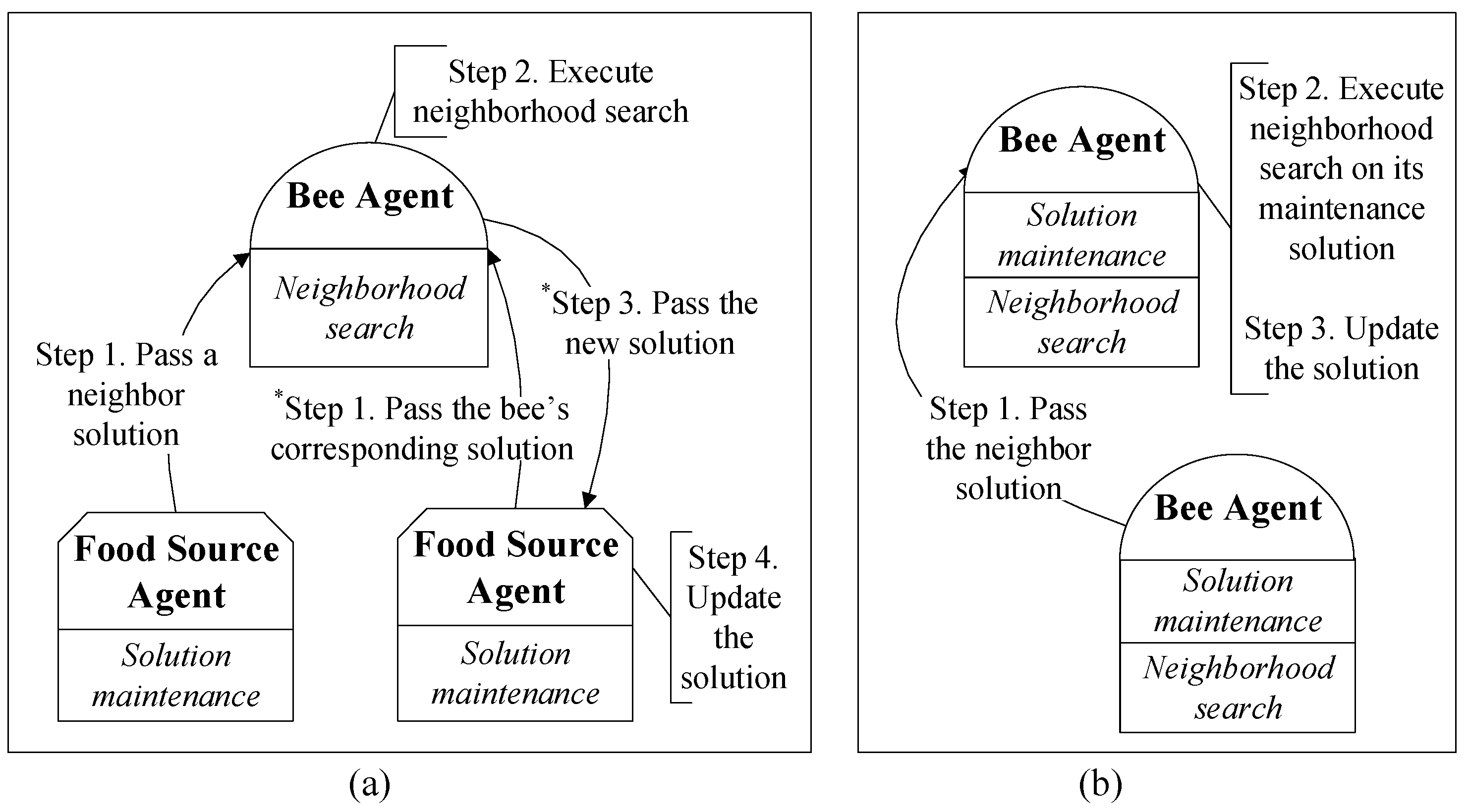
3.4. Computational Complexity

If the numbers of employed and onlooker bees number are both $BN$, the maximum iteration number is T, the parameter related to a scout bee’s behavior of abandoning a solution is $N_{\mathrm{limit}}$, a solution’s dimension (for example, the number of endmembers and clustering centers in the problem of endmember extraction and clustering) is $M$, and the number of parallel computing nodes is $C(C\le BN)$, the time complexity of the framework can be represented in

Table 1. The Time Complexity of the Framework.

	Complexity	Description
Initialization phase	$\frac{M\times BN}{C}$	Generate $BN$ solutions of $M$ dimensions in parallel.
Employed bee phase	$\frac{T\times BN\times g(*)}{C}$	Generate $BN$ new solutions by neighborhood search, and calculate the objective function values in $T$ iterations in parallel.
Onlooker bee phase	$\frac{T\times BN\times g(*)}{C}$
Scout bee phase	$BN$	Calculate $BN$ solutions’ fitness.
	$\frac{[\frac{T}{K}]\times M\times BN}{C}$	In the worst case, $BN$ bees abandon original solutions every $K$ iterations and generate new solutions of $M$ dimensions in parallel.
Total	$BN\times (1+\frac{(1+[\frac{T}{K}])\times M+2\times T\times g(*)}{C})$

, where $g(*)$ is the complexity of the RS optimization objective function value calculation.

3.5. Comparison

In the MA-based ABC proposed in [17], a food source agent is only responsible for a solution’s maintenance and a bee agent is only responsible for the neighborhood search (shown in Figure 4a). Because a bee agent does not store a solution, whenever it executes a neighborhood search in the employed and onlooker bee phases, it has to solicit two solutions from two different food source agents through the network (shown as step 1 in Figure 4a). Subsequently, the new generated solution should also be passed to its corresponding food source agent to update solutions (shown as step 3 in Figure 4a). The frequent communications in the MA-based ABC reduce the computational performance.

In the improved MA-based ABC framework proposed in this paper, each agent exhibits both behaviors (solution maintenance and neighborhood search), and its neighborhood search can be directly executed on its maintenance solution, which means that only one neighbor solution has to be passed to an agent in all of the employed phases (shown in Figure 4b) and parts of the onlooker bee phases (if one of the two randomly selected solutions for a bee happens to be maintained by the bee). Thus, the frequency of transferring solutions among agents will be effectively reduced, which is helpful for improving the efficiency of parallel computation.

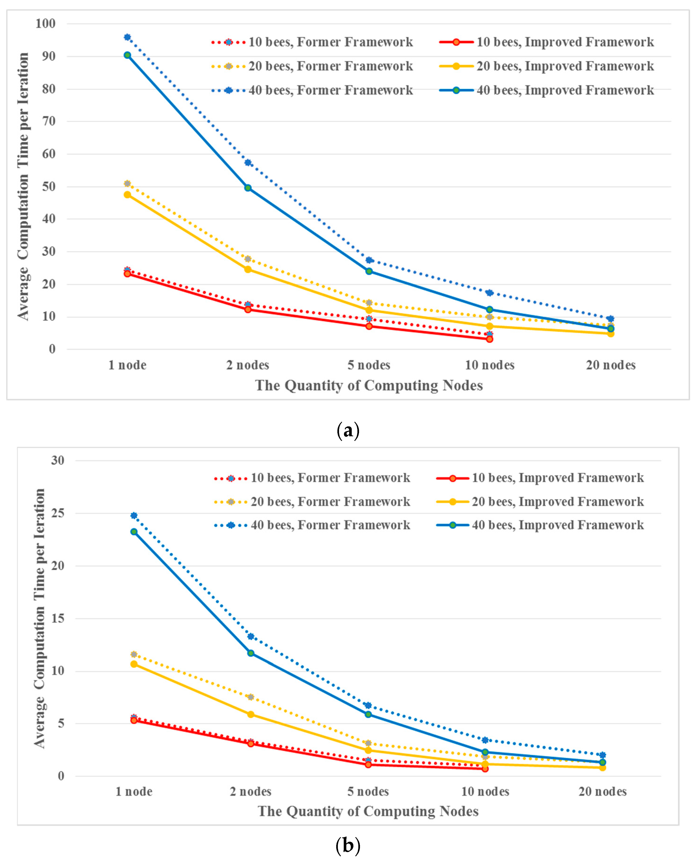
To quantitatively analyze the improvement, the number of transferred solutions among agents in one iteration can be listed as shown in

Table 2. The Number of Transferred Solutions among Agents in one Iteration.

Algorithm Phase	The Behaviors of Agents	The Former Framework in [17]	The Improved Framework in This Paper
Employed bee	The administrator agents passing solutions to each employed bee agent	$2BN$	$BN$(1)
	Each employed bee agent passing a solution to a food source agent	$BN$	0
	Passing solutions to the administrator agent	$BN$	$BN$
Onlooker bee	The admin agents passing solutions to onlooker bee agents	$2BN$	$BN$+$BN\times p_1$(2)
	Each onlooker bee agent passing a solution to a food source agent	$BN$	0
	Onlooker bee agents passing solutions to other bee agents	0	$BN\times p_2$(3)
	Passing solutions to the administrator agent	$BN$	$BN$
Sum		$8BN$	$4BN+2BN\times (P_1+P_2)$

Note: ⁽¹⁾ In the employed bee phase, because each bee agent maintains a solution, only one neighborhood solution has to be transferred from the administrator agent to each bee agent; thus, the number of transferred solutions among agents is $BN$, where $BN$ is the number of bees. ⁽²⁾ In the onlooker bee phase, two solutions ($X_k$ and $X_r$) must be transferred to each bee agent. If one of the two solutions happens to be the solution maintained by the bee agent, there is no need to transfer the solution. Fraction $p_1(0\le p_1\le 1)$ can be imported to describe the probability of this possibility. $p_1=\frac{N^{\prime }}{BN}$, where $N^{\prime }$ is the number of bees whose maintaining solution happens to be one of the two solutions in their onlookers’ neighborhood search. Thus, the total number of transferred solutions is $BN$+$BN\times p_1$. ⁽³⁾ For a bee agent, if its new generated solution $X^{\prime }$ is better than $X_k$, and $X_k$ is another bee agent’s maintaining solution, $X^{\prime }$ must be transferred. The fraction $p_2(0\le p_2\le 1)$ is defined to describe the probability of this possibility. Thus, the number of transferred solutions under such circumstances is $BN\times p_2$.

, which indicates that the improved framework proposed in this paper will spend less time on communication than the former framework [17] does, thus achieving higher efficiency.

4. Case Studies

To validate the effectiveness and efficiency of the proposed MA-based ABC approach while solving the computational challenges of RS optimization, an image clustering problem considering Markov random fields (MRFs) [5] and endmember extraction [16] are taken as case studies.

4.1. RS Optimization for Clustering

The model aims to minimize the total MRF classification discriminant function value, which can be summarized as the following optimization problem:

$$\begin{array}{cc}\min & U={\displaystyle \sum _{i=1}^n{U}_{i{\omega }_i}}\end{array}$$

(5)

$$s.t.{\omega }_i=\arg {\min }_j\left\{U_{ij}\right\}$$

(6)

$$U_{ij}=d_{ij}+\beta b_{ij}={\Vert {\mathbf{r}}_i-{\mathbf{c}}_j\Vert }_2+\beta {\displaystyle \sum _{\partial i}(1-}\delta (j,{\omega }_{\partial i}))$$

(7)

$$d_{ij}=\mathrm{d}({\mathbf{r}}_i,{\mathbf{c}}_j)={\Vert {\mathbf{r}}_i-{\mathbf{c}}_j\Vert }_2$$

(8)

$$b_{ij}={\displaystyle \sum _{\partial i}(1-}\delta (j,{\omega }_{\partial i}))$$

(9)

$$1\le j\le m$$

(10)

where $U_{ij}$ is the MRF classification discriminant function, a combination of spectral and spatial similarity (shown in (5)). The Euclidean distance $d_{ij}$ between the pixel ${\mathbf{r}}_i$ and the cluster center ${\mathbf{c}}_j$, shown in (8), reflects the degree of spectral similarity between ${\mathbf{r}}_i$ and class $X_j$. $b_{ij}$ represents the spatial similarity between pixel ${\mathbf{r}}_i$ and class $X_j$, which can be obtained by Function (9). $\partial i$ represents a pixel in the neighborhood of ${\mathbf{r}}_i$, ${\omega }_{\partial i}$ represents the class of that pixel in the neighborhood of ${\mathbf{r}}_i$, and $\delta (\cdot ,\cdot )$ represents the Kronecker function. The parameter $\beta$ is used to control the influence of the spatial information during classification, $i$ is the number of pixels in the RS image, and $j$ is the number of clusters. The objective function calculation of this model is detailed in [5].

4.2. RS Optimization for Endmember Extraction

One RS optimization for endmember extraction can be modeled to minimize the volume of endmembers and the root-mean-square error (RMSE) value of the extracted results. The model can be expressed as follows.

$$\min f(E)=V({\left\{{\tilde{\mathbf{e}}}_j\right\}}_{j=1}^M)+\mu RMSE({\left\{{\tilde{\mathbf{r}}}_i\right\}}_{i=1}^N,{\left\{{\tilde{\mathbf{e}}}_j\right\}}_{j=1}^M)$$

(11)

$${\tilde{\mathbf{r}}}_i={\displaystyle \sum _{j=1}^M{\alpha }_{ij}{\tilde{\mathbf{e}}}_j}+{\epsilon }_i$$

(12)

$${\displaystyle \sum _{j=1}^M{\alpha }_{ij}=1,\forall i}$$

(13)

$${\alpha }_{ij}\ge 0,\forall i,\forall j$$

(14)

$$V({\left\{{\tilde{\mathbf{e}}}_j\right\}}_{j=1}^M)=\frac{1}{(M-1)!}\left|\det \left(\left[\begin{array}{cccc}1& 1& \cdots & 1\\ {\tilde{\mathbf{e}}}_1& {\tilde{\mathbf{e}}}_2& \cdots & {\tilde{\mathbf{e}}}_M\end{array}\right]\right)\right|$$

(15)

$$RMSE({\left\{{\tilde{\mathbf{r}}}_i\right\}}_{i=1}^N,{\left\{{\tilde{\mathbf{e}}}_j\right\}}_{j=1}^M)=\frac{1}{N}{\displaystyle \sum _{i=1}^N}||{\tilde{\mathbf{r}}}_i-{\displaystyle \sum _{j=1}^M}{\widehat{\alpha }}_{ij}{\tilde{\mathbf{e}}}_j|{|}_2$$

(16)

${\left\{{\tilde{\mathbf{e}}}_j\right\}}_{j=1}^M$ represents the $M$ endmembers in the dimension-reduced hyperspectral image ${\left\{{\tilde{\mathbf{r}}}_i\right\}}_{i=1}^N$ with $N$ pixels; ${\alpha }_{ij}$ is the abundance, which represents the proportion of the $j$-th endmember in the $i$-th pixel; and ${\epsilon }_i$ is the random error. $V({\left\{{\tilde{\mathbf{e}}}_j\right\}}_{j=1}^M)$ is the volume of the simplex whose vertices are ${\left\{{\tilde{\mathbf{e}}}_j\right\}}_{j=1}^M$.

5. Experiments

5.1. Experimental Data

5.1.1. Dataset 1

The Pavia dataset with a spatial resolution of 1.3 m was collected by the Reflective Optics System Imaging Spectrometer (ROSIS) over the University of Pavia, Italy, in 2001. The dataset contains 103 bands (after the removal of the water vapor absorption bands and bands with a low signal-to-noise ratio (SNR)) with a wavelength range of 430–860 nm and covers an area of 610 × 340 pixels. A false color composite image (bands 80, 45, and 10) is shown in Figure 5a. The ground truth dataset, which contains nine classes, is shown in Figure 5b.

5.1.2. Dataset 2

The Indian Pine dataset with a spatial resolution of 20 m was obtained by the airborne visible/infrared imaging spectrometer (AVIRIS) in 1992. The dataset contains 169 bands (after the removal of the water vapor absorption bands and low-SNR bands) with a wavelength range of 400–2500 nm and covers an area of 145 × 145 pixels. A false color composite image (bands 54, 33, and 19) is shown in Figure 6a. The ground truth dataset, which contains 16 classes, is shown in Figure 6b.

5.2. Experimental Design

5.2.1. Comparison Experiments

All experiments were carried out in multiple computing nodes with the same hardware configuration shown in

Table 3. The Hardware Configuration Used in the Experiments.

Number of Cores	Number of Threads	CPU (GHz)	Bus Speed (MHz)	Multiplier	RAM (GB)
4	4	3.4	100	30	8

. The MA framework was developed in the language of Java by using the Java Agent Development (JADE) platform, and all objective function calculations were coded in MATLAB and imported into the MA framework as a JAR package.

For each dataset, two comparison experiments were designed to validate the MA-based ABC approach in two respects: optimal solution accuracy and calculation efficiency. The accuracy of the optimal solutions is evaluated by comparing with the original algorithms implemented on a single computer. The calculation efficiency is evaluated by comparing with the MA framework proposed in [17].

Notably, weight values are involved in both case studies; for example, the $\beta$ in formulation (7) and $\mu$ in formulation (1), which affect the solution quality and the convergence speed. However, the goal of the experiments designed here is to prove that the solution accuracy will not decrease under different frameworks with the same parameter settings but that the calculation efficiency will be improved. Thus, both the weight values in the two case studies are set to 1000 according to [5]. It should be noted that the weight value setting may not be the best choice for all RS datasets and case studies.

5.2.2. Evaluation Criteria

Two types of criteria are used to evaluate the accuracy and efficiency.

(1) Accuracy criteria

• RS optimization for clustering

For the RS optimization problem of image clustering considering MRF, four criteria are chosen to evaluate the results’ accuracy: (1) purity, (2) normalized mutual information (NMI), (3) adjusted random index (ARI), and (4) segmentation accuracy (SA).

Purity is a simple and transparent measure for evaluating how well the clustering matches the ground truth data, which can be calculated as follows:

$$purity(C,G)=\frac{1}{N}{\displaystyle \sum _j\underset{k}{\max }|{\mathbf{c}}_j\cap g_k|}$$

(17)

where $C=\{{\mathbf{c}}_1,{\mathbf{c}}_2,\cdots {\mathbf{c}}_J\}$ is the set of clusters and $G=\{g_1,g_2,\cdots g_K\}$ is the set of classes of the ground truth. ${\mathbf{c}}_j$ is the set of image pixels in cluster $j$, and $g_k$ is the set of pixels in class $k$. The closer the value of purity is to 1, the better the cluster result is. High purity is easy to achieve when the number of clusters is large, but purity cannot be used to trade off the quality of clustering against the number of clusters.

To make this tradeoff, NMI can be introduced.

$$NMI(C,G)=\frac{{\displaystyle \sum _j{\displaystyle \sum _{k}P({\mathbf{c}}_j\cap g_k)\log \frac{P({\mathbf{c}}_j\cap g_k)}{P({\mathbf{c}}_j)P(g_k)}}}}{-{\displaystyle \sum _{j}P({\mathbf{c}}_j)\log P({\mathbf{c}}_j)}}$$

(18)

where $P({\mathbf{c}}_j)$,$P(g_k)$, and $P(c_j\cap g_k)$ are the probabilities of a pixel being in cluster ${\mathbf{c}}_j$, class $g_k$, and the intersection of ${\mathbf{c}}_j$ and $g_k$, respectively. The value of NMI is normalized within the range [0,1]. A large value of NMI corresponds to a high-quality result.

ARI is used to evaluate the degree of consistency between the classification results and the test samples. The clustering result and the ground truth data are two different class partitions of pixels. For an image with $n$ pixels, a contingency table, such as that shown in

Table 4. Contingency Table of the Clustering Result and Ground Truth Data.

	Ground Truth Data	Pixel Pair with the Same Class Label	Pixel Pair with Different Class Labels
Clustering Result
Pixel pair with the same class label		$a$	$b$
Pixel pair with different class labels		$c$	$d$

, can be obtained by calculating the parameters a, b, c and d according to [28].

The ARI is calculated as follows:

$$ARI=\frac{\left(\begin{array}{l}n\\ 2\end{array}\right)(a+d)-[(a+b)(a+c)+(c+d)(b+d)]}{{\left(\begin{array}{l}n\\ 2\end{array}\right)}^2-[(a+b)(a+c)+(c+d)(b+d)]}$$

(19)

The value of the ARI lies between 0 and 1. The higher the ARI value is, the better the classification result is.

The criteria for SA, an evaluation index for the classification accuracy, can be obtained by the power of spectral discrimination (PWSD), which is one way to measure the degree of difference between two different cluster centers for the same pixel. For pixel ${\mathbf{x}}_i$ and cluster centers ${\mathbf{c}}_{j_1}$ and ${\mathbf{c}}_{j_2}$, the PWSD $\Omega ({\mathbf{c}}_{j_1},{\mathbf{c}}_{j_2};{\mathbf{x}}_i)$ is as follows:

$$\Omega ({\mathbf{c}}_{j_1},{\mathbf{c}}_{j_2};{\mathbf{x}}_i)=\max \{\frac{SAM({\mathbf{c}}_{j_1},{\mathbf{x}}_i)}{SAM({\mathbf{c}}_{j_2},{\mathbf{x}}_i)},\frac{SAM({\mathbf{c}}_{j_2},{\mathbf{x}}_i)}{SAM({\mathbf{c}}_{j_1},{\mathbf{x}}_i)}\}$$

(20)

where $SAM({\mathbf{c}}_j,{\mathbf{x}}_i)={\cos }^{-1}\left(\frac{{\mathbf{c}}_j^T\cdot {\mathbf{x}}_i}{{\Vert {\mathbf{c}}_j\Vert }_2\cdot {\Vert {\mathbf{x}}_i\Vert }_2}\right)$ is the spectral angle distance between ${\mathbf{x}}_i$ and ${\mathbf{c}}_j$. For an RS image, SA can be formulated as follows [29]:

$$SA=\frac{1}{n}{\displaystyle \sum _{i=1}^n\sum _{j=1,j\ne {\omega }_i}^m\frac{\Omega ({\mathbf{c}}_{{\omega }_i},{\mathbf{c}}_j;{\mathbf{x}}_i)}{m-1}}$$

(21)

As the distinction between cluster centers and pixels increases, the corresponding values of PWSD and SA also increase. Therefore, large SA and PWSD values correspond to a high-quality clustering result.

• RS optimization for endmember extraction

For the RS optimization problem of endmember extraction, the RMSE is a commonly used accuracy criterion. The RMSE quantifies the error between the original hyperspectral image and the remixed image, which represents the generalized degree of image information provided by the extracted endmembers [30]. The RMSE is calculated by Equation (16).

(2) Efficiency criteria

We use the classical notions of speedup and computational efficiency.

The speedup $S_C=T_1/T_C$ of a distributed application measures how much faster the algorithm runs when it is implemented on multiple computing nodes than it does on a single computing node. The computational efficiency $e_C=S_C/C$ measures the average speedup value in a computation clustering environment. Here, $C$ is the number of computing nodes, $T_1$ is the execution time on a single computing node, and $T_C$ is the algorithm’s execution time on $C$ computing nodes.

6. Results

6.1. Accuracy

According to the logic of the ABC algorithm, there is no difference in accuracy between the improved framework reported in this paper and the algorithm without MA technology. In other words, the different parallel design will not affect the algorithm’s accuracy, which is validated in this section.

6.1.1. Accuracy of Clustering

The MA-based ABC framework coupled with the ABC-MRF-cluster algorithm in [5] and the ABC-MRF-cluster without using MA technology were run 10 times for comparison.

The median, mean, and standard deviation of the objective function and the t-test value are listed in

Table 5. Accuracy Statistics of the multiagent (MA)-based ABC Framework and the ABC-MRF-cluster in [5] for Dataset 1.

	ARI		PWSD		NMI		Purity
	MA-Based ABC Framework	ABC-MRF-Cluster	MA-Based ABC Framework	ABC-MRF-Cluster	MA-Based ABC Framework	ABC-MRF-Cluster	MA-Based ABC Framework	ABC-MRF-Cluster
Median Value	0.3088	0.3189	5.9785	5.8356	0.5505	0.5595	0.5796	0.5916
Mean Value	0.3113	0.3212	5.8737	5.8034	0.5552	0.5590	0.5843	0.5891
Standard Deviation	0.0174	0.0229	0.5475	1.3014	0.0111	0.0112	0.0192	0.0213
p-value	0.0930		0.8182		0.2280		0.4029

MRF, Markov random field.

and

Table 6. Accuracy Statistics of the MA-based ABC Framework and the ABC-MRF-cluster in [5] for Dataset 2.

	ARI		PWSD		NMI		Purity
	MA-Based ABC Framework	ABC-MRF-Cluster	MA-Based ABC Framework	ABC-MRF-Cluster	MA-Based ABC Framework	ABC-MRF-Cluster	MA-Based ABC Framework	ABC-MRF-Cluster
Median Value	0.2164	0.2148	6.2587	6.0156	0.4458	0.4460	0.4013	0.3985
Mean Value	0.2210	0.2206	6.5233	6.5073	0.4510	0.4492	0.4118	0.4031
Standard Deviation	0.0132	0.0145	0.8342	1.3508	0.0119	0.0095	0.0323	0.0238
p-value	0.9439		0.9750		0.7061		0.4996

. The values of the ARI and PWSD are similar and remain stable, which means that the accuracy of ABC-MRF-cluster classification accelerated by MA technology is nearly the same as that of ABC-MRF-cluster classification executed on a single computer. Additionally, both standard deviations of the objective function, which are much smaller than the mean and median value, prove the algorithm’s stability. Furthermore, the t-test values, which can be used for evaluation if two sets of data are significantly different from each other, are calculated. The p-values of all criteria between the ABC-MRF-cluster and the MA-based ABC are much greater than the threshold value of 0.05, which proves that there is no notable difference between the optimization results of the MA-based ABC framework and the ABC algorithm without MA technology. Therefore, we can conclude that the MA-based approach will not affect the optimization accuracy.

6.1.2. Accuracy of Endmember Extraction (EE)

The MA-based ABC framework improved upon in this paper coupled with the ABC-EE algorithm in [16] and the ABC-EE without using MA technology were run 10 times for comparison. The accuracy statistics are shown in

Table 7. Accuracy Statistics of the MA-based ABC Framework and ABC-EE in [16].

RMSE	RMSE for Dataset 1		RMSE for Dataset 2
	MA-based ABC Framework	ABC-EE	MA-Based ABC Framework	ABC-EE
Median Value	386.54	390.24	110.49	123.99
Mean Value	375.13	393.83	125.30	139.85
Standard Deviation	151.98	133.11	41.32	49.03
p-value	0.54		0.19

EE, endmember extraction.

. The p-value of the RMSE between the ABC-MRF-cluster and MA-based ABC are greater than the threshold value of 0.05, which also proves that there is no notable difference between the optimization results of the MA-based ABC framework and the ABC algorithm without MA technology.

6.2. Efficiency

6.2.1. Efficiency of Clustering

(1) Comparison with the framework proposed in [17]

To validate the improvement in the enhanced MA-based ABC framework, a comparison with the former framework proposed in [17] was made to solve the same RS optimization in the same computing environment and under the same parameter settings. When performing all the experiments, all of the bee agents were uniformly distributed on each computation node and the administrator agent was randomly distributed on one node.

The comparison results are shown in

Table 8. Efficiency Statistics of the Improved MA-based ABC Framework and the Framework Proposed in [17] for Clustering.

Computing Environment	Population of Bees	Average Computation Time per Iteration for Dataset 1				Average Computation Time per Iteration for Dataset 2
		Former Framework (second)	Improved Framework (second)	Promotion GAP	Average Promotion GAP	Former Framework (second)	Improved Framework (second)	Promotion GAP	Average Promotion GAP
1 Node Computation	10	24.43	23.36	4.58%	5.83%	5.59	5.34	4.75%	6.57%
	20	50.91	47.66	6.82%		11.58	10.69	8.32%
	40	96.07	90.56	6.08%		24.78	23.24	6.64%
2 Nodes Computation	10	13.72	12.20	12.49%	13.71%	3.30	3.09	6.88%	16.13%
	20	27.79	24.56	13.13%		7.54	5.89	27.85%
	40	57.48	49.75	15.52%		13.31	11.72	13.65%
5 Nodes Computation	10	9.40	7.16	31.24%	21.72%	1.54	1.14	34.82%	25.91%
	20	14.35	12.05	19.12%		3.16	2.46	28.71%
	40	27.54	23.99	14.79%		6.73	5.89	14.21%
10 Nodes Computation	10	4.62	3.28	40.92%	40.02%	1.05	0.74	42.41%	48.93%
	20	9.98	7.24	37.77%		1.88	1.20	56.09%
	40	17.47	12.35	41.38%		3.47	2.34	48.30%
20 Nodes Computation	10	-	-	-	50.29%	-	-	-	56.91%
	20	7.41	4.94	50.05%		1.35	0.85	59.45%
	40	9.54	6.34	50.52%		2.05	1.33	54.37%

Note: “-” indicates that no experiments are carried out under the corresponding circumstances.

. In the one-node computation environment, the computation time consumed per iteration of the improved framework is shorter than the former framework, with an average computing efficiency promotion gap of 5.83% for dataset 1 and 6.57% for dataset 2. With the increase in the number of computation nodes, the average efficiency gap between the improved and the former framework becomes increasingly large, exceeding 50% when there are 20 nodes for dataset 1 and dataset 2. The results indicate that the improved MA-based ABC framework is more efficient than the framework proposed in [17].

(2) Influence of the quantity of computation nodes

To better analyze the influence of the quantity of computation nodes participating in the MA-based ABC framework for RS optimization, a series of comparison experiments were performed by setting the population of ABC to 10, 20, and 40 in different computation environments with 1, 2, 5, 10, and 20 nodes. Each experiment was performed 10 times. The statistical results are shown in Figure 7 and Table 8.

As shown in Figure 7, regardless of how many bees are involved in the computation, the average computation time per iteration decreases dramatically as the number of computation nodes increases. Moreover, each bee’s average computation time in one iteration was calculated (Table 8). This finding indicates that the speedup of the improved MA-based ABC algorithm increases significantly with the increase in the number of nodes in the parallel computation environment. However, the computational efficiency of each node’s performance nonlinearly decreases due to the increased communication cost among nodes within the network when adding more nodes.

The statistical values of the improved MA-based ABC framework’s efficiency criteria are presented in

Table 9. Statistical Values of the Improved MA-based ABC Framework’s Efficiency Criteria.

Computing Environment	Dataset 1			Dataset 2
	Average Computation Time per Iteration per Bee	Speedup	Computational Efficiency	Average Computation Time per Iteration per Bee	Speedup	Computational Efficiency
1 node	2.3277588	1.00	1.00	0.54966283	1.00	1.00
2 nodes	1.2306427	1.89	0.95	0.298756997	1.84	0.92
5 nodes	0.6394509	3.64	0.73	0.128231976	4.29	0.86
10 nodes	0.3329333	6.99	0.70	0.064166337	8.57	0.86
20 nodes	0.2026791	11.48	0.57	0.037837861	14.53	0.73

. When increasing the number of computing nodes, the speedup increases significantly since all calculations can be carried out at multiple nodes concurrently. In addition, the results also show that with the increase in the number of nodes, the computational efficiency of a node decreases, as a higher network communication cost to other nodes is generated.

6.2.2. Efficiency of Endmember Extraction

Let there be 60 bees in experiments for both datasets; a comparison between this improved framework and the former framework in [17] can be made in different parallel environments with 1, 2, 5, 10, and 20 computing nodes.

The efficiency statistics of these two frameworks for endmember extraction are recorded in

Table 10. Efficiency Statistics of the Improved MA-based ABC Framework and the Former Framework Proposed in [17] for Endmember Extraction.

Computing Environment	Computation Time per Iteration for Dataset 1			Computation Time per Iteration for Dataset 2
	Former Framework (second)	Improved Framework (second)	Promotion Gap	Former Framework (second)	Improved Framework (second)	Promotion Gap
1 node	20.73	20.31	2.03%	26.00	25.58	1.66%
2 nodes	10.39	10.18	2.08%	13.36	13.18	1.40%
5 nodes	4.31	4.13	4.35%	5.92	5.32	11.24%
10 nodes	2.26	2.06	9.31%	3.01	2.68	12.19%
20 nodes	1.19	1.03	15.13%	1.68	1.42	18.36%

. Clearly, the computation time per iteration of the improved framework is shorter than that of the former framework for both datasets. In particular, as more nodes are added in the computing environment, the efficiency advantage of the improved framework becomes more prominent.

The speedup and computational efficiency are calculated as depicted in Figure 8. By analyzing lines of the same color, it can be found that, with the increase in the number of computing nodes, the speedup increases dramatically, but the computational efficiency decreases because of the rising communication cost among different nodes. Comparing lines containing the same shapes (circles or rectangles) indicates that the improved framework outperforms the former framework with a higher speedup value and a lower efficiency descent rate. By observing lines of the same type, it can be observed that both the speedup and computational efficiency tendencies of dataset 1 are much better than those of dataset 2. The reason is that the amount of time used to calculate the objective function value for dataset 1 is less than that used to calculate dataset 2 after sampling, and the communication cost for dataset 1 occupies a higher proportion of the total calculation cost, which results in a greater computational improvement by saving on the same communication cost.

7. Discussion

7.1. Stability

In this paper, the failure of a single computing node does not lead to the failure of the overall computation, which provides the proposed computational framework with good computational stability. Such stability is achieved by predefining a time limit $t$ for each node’s calculation. When the management agent does not receive the results returned by bee agents within the time after a calculation instruction is sent, it can be concluded that the node’s calculation or the network communication failed. In this case, the administrator agent can resend calculation instructions to obtain the correct calculation results from bee agents.

7.2. Scalability

The computational framework proposed maintains good scalability. Any newly added bee agent can perform optimization together with other previously deployed bee agents as long as the agent is deployed in the same communication network and registered at the management agent. Therefore, the number of computation nodes of the parallel computation is easily increased, and the computation scale is easily expanded. Similarly, if certain computing nodes are not needed to participate in parallel computing, their network IP addresses can be deleted from the management agent.

7.3. Flexibility

Hyperspectral RS image clustering and endmember extraction were applied to validate the performance of an MA-based ABC approach. However, the parallel computing framework proposed in this paper can be easily applied to many other RS optimization problems. In this framework, all the behaviors of the managing agent, as well as the communication behaviors of the bee agents and the neighborhood search behaviors, are universal and can be used for most RS optimization problems. We can solve different RS optimization problems by modifying each bee agent’s objective function calculation method and its required parameters. Therefore, the parallel computing framework proposed in this paper has good flexibility.

8. Conclusions

In this paper, an improved parallel processing approach involving the integration of an ABC optimization approach and multiagent technology is proposed. Taking hyperspectral RS image clustering and endmember extraction as examples, two types of agents are designed: an administrator agent and multiple bee agents. By executing the behaviors of each agent and the communication among agents, an optimal result without sacrificing accuracy can be obtained by parallel computation with dramatically increased efficiency. Moreover, a series of experiments proves that the improved MA-based ABC framework can achieve a greater enhancement in parallel computational efficiency than the framework proposed in [17] can. Moreover, the integration of MA and GPU technology by offloading each individual’s behaviors to the GPU’s arithmetic logic units under this MA-based ABC framework could be a more efficient approach, which should be further studied.

References

1. Richards, J.A. Remote Sensing Digital Image Analysis—An Introduction; Springer: Berlin/Heidelberg, Germany, 2012. [Google Scholar]
2. Wang, Q.; Meng, Z.; Li, X. Locality adaptive discriminant analysis for spectral–spatial classification of hyperspectral images. IEEE Geosci. Remote Sens. Lett. 2017, 14, 2077–2081. [Google Scholar] [CrossRef]
3. Peng, X.; Feng, J.; Xiao, S.; Yau, W.; Zhou, J.T.; Yang, S. Structured autoencoders for subspace clustering. IEEE Trans. Image Process. 2018, 27, 5076–5086. [Google Scholar] [CrossRef] [PubMed]
4. Peng, X.; Yu, Z.; Yi, Z.; Tang, H. Constructing the l2-graph for robust subspace learning and subspace clustering. IEEE Trans. Cybern. 2017, 47, 1053–1066. [Google Scholar] [CrossRef] [PubMed]
5. Sun, X.; Yang, L.; Gao, L.; Zhang, B.; Li, S.; Li, J. Hyperspectral image clustering method based on artificial bee colony algorithm and markov random fields. J. Appl. Remote Sens. 2015, 9. [Google Scholar] [CrossRef]
6. Zhang, B.; Gao, J.; Gao, L.; Sun, X. Improvements in the ant colony optimization algorithm for endmember extraction from hyperspectral images. IEEE J. Sel. Top. Appl. Earth Obs. Remote Sens. 2013, 6, 522–530. [Google Scholar] [CrossRef]
7. Zou, J.; Lan, J.; Shao, Y. A hierarchical sparsity unmixing method to address endmember variability in hyperspectral image. Remote Sens. Basel 2018, 10, 738. [Google Scholar] [CrossRef]
8. Zhang, B.; Sun, X.; Gao, L.; Yang, L. Endmember extraction of hyperspectral remote sensing images based on the discrete particle swarm optimization algorithm. IEEE Trans. Geosci. Remote Sens. 2011, 49, 4173–4176. [Google Scholar] [CrossRef]
9. Ghamisi, P.; Couceiro, M.S.; Ferreira, N.M.; Kumar, L. Use of darwinian particle swarm optimization technique for the segmentation of remote sensing images. In Proceedings of the 2012 IEEE International Geoscience and Remote Sensing Symposium, Munich, Germany, 22–27 July 2012; pp. 4295–4298. [Google Scholar]
10. Jain, A.K. Data clustering: 50 years beyond k-means. Pattern Recogn. Lett. 2010, 31, 651–666. [Google Scholar] [CrossRef]
11. Zhang, B.; Sun, X.; Gao, L.; Yang, L. An innovative method of endmember extraction of hyperspectral remote sensing image using elitist ant system (EAS). In Proceedings of the 2012 International Conference on Industrial Control and Electronics Engineering, Xi’an, China, 23–25 August 2012; pp. 1625–1627. [Google Scholar]
12. Zhang, B.; Sun, X.; Gao, L.; Yang, L. Endmember extraction of hyperspectral remote sensing images based on the ant colony optimization (ACO) algorithm. IEEE Trans. Geosci. Remote Sens. 2011, 49, 2635–2646. [Google Scholar] [CrossRef]
13. Karaboga, D.; Ozturk, C. A novel clustering approach: Artificial bee colony (ABC) algorithm. Appl. Soft Comput. 2011, 11, 652–657. [Google Scholar] [CrossRef]
14. Hancer, E.; Ozturk, C.; Karaboga, D. Artificial bee colony based image clustering method. In Proceedings of the 2012 IEEE Congress on Evolutionary Computation, Brisbane, QLD, Australia, 10–15 June 2012. [Google Scholar]
15. Bhandari, A.K.; Soni, V.; Kumar, A.; Singh, G.K. Artificial bee colony-based satellite image contrast and brightness enhancement technique using dwt-svd. Int. J. Remote Sens. 2014, 35, 1601–1624. [Google Scholar] [CrossRef]
16. Sun, X.; Yang, L.; Zhang, B.; Gao, L.; Gao, J. An endmember extraction method based on artificial bee colony algorithms for hyperspectral remote sensing images. Remote Sens. Basel 2015, 7, 16363–16383. [Google Scholar] [CrossRef]
17. Yang, L.; Sun, X.; Peng, L.; Yao, X.; Chi, T. An agent-based artificial bee colony (ABC) algorithm for hyperspectral image endmember extraction in parallel. IEEE J. Sel. Top. Appl. Earth Obs. Remote Sens. 2015, 8, 4657–4664. [Google Scholar] [CrossRef]
18. Tan, Y.; Ding, K. A survey on gpu-based implementation of swarm intelligence algorithms. IEEE Trans. Cybern. 2016, 46, 2028–2041. [Google Scholar] [CrossRef] [PubMed]
19. Dawson, L.; Stewart, I.A. Accelerating ant colony optimization-based edge detection on the GPU using CUDA. In Proceedings of the 2014 IEEE Congress on Evolutionary Computation (CEC), Beijing, China, 6–11 July 2014; pp. 1736–1743. [Google Scholar]
20. Kristiadi, A.; Pranowo, P.; Mudjihartono, P. Parallel particle swarm optimization for image segmentation. In Proceedings of the Second International Conference on Digital Enterprise and Information Systems (DEIS2013), Kuala Lumpur, Malaysia, 4–6 March 2013; pp. 129–135. [Google Scholar]
21. Nascimento, J.M.P.; Bioucas-Dias, J.M.; Alves, J.M.R.; Silva, V.; Plaza, A. Parallel hyperspectral unmixing on gpus. IEEE Geosci. Remote Sens. Lett. 2013, 11, 666–670. [Google Scholar] [CrossRef]
22. Owens, J.D.; Houston, M.; Luebke, D.; Green, S.; Stone, J.E.; Phillips, J.C. GPU computing. Proc. IEEE 2008, 96, 879–899. [Google Scholar] [CrossRef]
23. Karaboga, D.; Gorkemli, B.; Ozturk, C.; Karaboga, N. A comprehensive survey: Artificial bee colony (ABC) algorithm and applications. Artif. Intell. Rev. 2014, 42, 21–57. [Google Scholar] [CrossRef]
24. Bellifemine, F.; Caire, G.; Greenwood, D. Developing Multi-Agent System with JADE; John Wiley & Sons Ltd.: Hoboken, NJ, USA, 2007. [Google Scholar]
25. Xiang, W.; Lee, H.P. Ant colony intelligence in multi-agent dynamic manufacturing scheduling. Eng. Appl. Artif. Intell. 2008, 21, 73–85. [Google Scholar] [CrossRef]
26. Jennings, N.R. On agent-based software engineering. Artif. Intell. 2000, 2, 277–296. [Google Scholar] [CrossRef]
27. Leung, C.W.; Wong, T.N.; Mak, K.L.; Fung, R.Y.K. Integrated process planning and scheduling by an agent-based ant colony optimization. Comput. Ind. Eng. 2010, 59, 166–180. [Google Scholar] [CrossRef]
28. Santos, J.; Embrechts, M. On the use of the adjusted rand index as a metric for evaluating supervised classification. In Lecture Notes in Computer Science; Alippi, C., Polycarpou, M., Panayiotou, C., Ellinas, G., Eds.; Springer: Berlin/Heidelberg, Germany, 2009; Volume 5769, pp. 175–184. [Google Scholar]
29. Bilgin, G.; Erturk, S.; Yildirim, T. Unsupervised classification of hyperspectral-image data using fuzzy approaches that spatially exploit membership relations. IEEE Geosci. Remote Sens. Lett. 2008, 5, 673–677. [Google Scholar] [CrossRef]
30. Plaza, A.; Martinez, P.; Perez, R.; Plaza, J. A quantitative and comparative analysis of endmember extraction algorithms from hyperspectral data. IEEE Trans. Geosci. Remote Sens. 2004, 42, 650–663. [Google Scholar] [CrossRef]
Figure 1. The procedure of the artificial bee colony (ABC) algorithm.
Remotesensing 11 00152 g001
Figure 2. Agents’ role design.
Remotesensing 11 00152 g002
Figure 3. The overall workflow of agents’ behaviors for remote sensing (RS) clustering.
Remotesensing 11 00152 g003
Figure 4. The major steps in generating a new solution. (a) The approach reported in [17] and (b) an improved version of (a). The steps labeled with * in (a) are redundant with (b).
Remotesensing 11 00152 g004
Figure 5. The Pavia dataset: (a) a false color composite image and (b) the ground truth.
Remotesensing 11 00152 g005
Figure 6. The Indian Pine dataset: (a) a false color composite image and (b) the ground truth.
Remotesensing 11 00152 g006
Figure 7. The average computation time per iteration for different numbers of bees and computing nodes. (a) Dataset 1 and (b) Dataset 2.
Remotesensing 11 00152 g007
Figure 8. The speedup and computational efficiency of the improved MA-based ABC framework.
Remotesensing 11 00152 g008