Recent Large Scale Environmental Changes in the Mediterranean Sea and Their Potential Impacts on Posidonia Oceanica

Abstract

Climate related changes can have significant effects on Posidonia oceanica, an endemic seagrass species of the Mediterranean Sea (MEDIT). This seagrass is very important for many aspects of functioning of the sea but there is an increasing number of reports about the ongoing loss of its biomass and area coverage. We analysed multiyear data of the sea surface temperature (SST), sea level anomalies, ocean colour MODIS-A and ERA-Interim reanalysis. The results provide a description of current environmental conditions in the MEDIT and their spatial and temporal variability, including long-term trends. We defined regions where the extent of the P. oceanica meadows may be limited by specific environmental conditions. Light limitation is more severe near the northern and western coasts of the MEDIT, where the vertical diffuse attenuation coefficient is large. In the zone extending from the Gulf of Lion towards the south, significant wave heights reach large values. Wave action may destroy the plants and as a result the shallow water depth limit of P. oceanica meadows is most likely deeper here than in other regions. The highest SST values are documented in the south-eastern part of the Mediterranean Sea. In this area P. oceanica meadows are more endangered by the climate warming than in other regions where SSTs are lower. The absence of P. oceanica meadows in the south-eastern edge of the Mediterranean Sea can be attributed to high temperatures. Our conclusions are partly confirmed by the information about P. oceanica from the literature but more monitoring efforts are needed to fully describe current extent of the meadows and their shifts. Results presented in this paper can help with designing special programs to confirm the role of environmental conditions on the spatial distribution of P. oceanica and their future trends in the Mediterranean Sea.

1. Introduction

The Mediterranean Sea (MEDIT) extends from 9° to 42°E and from 30° to 47°N and can be divided into several sub-basins (Figure 1). On the west, the sea is connected to the Atlantic Ocean through the Strait of Gibraltar, while on the east it is connected by the Dardanelles Strait to the Aegean and Black Sea. The Mediterranean Sea is important for economical and societal reasons. In recent years, a significant increase of urban developments took place in its coastal zones. Tourism and recreational sports have become a growing industry. In addition, there is a steady influx of new residents moving here from different European countries to spend their retirement. It is important to monitor what are the most significant environmental changes taking place in this region.

MEDIT region is a climate change hotspot [1]. This is manifested by stronger increase in air (AT) and sea surface (SST) temperatures than globally averaged trends. The rising rate of increase of global temperatures has stimulated a strong interest in developing useful methods for large-scale monitoring of climate-related environmental changes. Very efficient tools for this kind of research are satellite techniques. At present, it is well known that efforts to develop such techniques have been very successful since multiyear time series of different kinds of oceanographic (e.g., sea surface temperature, sea surface height, ocean colour, salinity, significant wave height), atmospheric (e.g., air temperature, moisture, clouds, precipitation) and land (e.g., vegetation index, soil moisture) data have been collected and validated. It is now possible to analyse these data and draw quantitative conclusions about the most important transformations taking place on Earth due to climate change. Our paper is dedicated to this type of research. In particular, using data from satellite observations, we want to exploit the links between climate change and transformations in the ecological status of the Mediterranean Sea. One of the unique aspects of our approach is that we apply interdisciplinary satellite data, while most of the previous research has been usually focused on one specific type of data (for example either ocean colour or sea level).

Environmental changes currently taking place in the Mediterranean Sea can have a range of possible impacts on ecological status of this region. Here we will focus on marine seagrass Posidonia oceanica (L.) Delile, an endemic seagrass species of the Mediterranean Sea. It grows between the depths of 0.5 and 45 m and covers an estimated surface area between 2.5 and 5 million ha, which is approximately 1–2% of the 0–50 m depth zone [2]. P. oceanica is very important for many aspects of functioning of the Mediterranean Sea [3]. Seagrass beds are enormously productive ecosystems. They provide for associated species shelter and food, thanks to relatively high rate of primary production. As a result, Posidonia oceanica meadows support commercially and recreationally valued fisheries. In addition, they slow down water movements, trap sediments and increase resistance to coastal erosion. What is more, seagrass meadows produce and store significant amounts of carbon [4,5,6]. It has been estimated that although all seagrass meadows cover only about 0.1 to 0.2% of the global ocean floor, they are associated with up to 18% of the total oceanic carbon burial [4,7]. About 10 Pg C of carbon sequestered by seagrasses is stored in the top 1 m of seagrass sediments [7]. Thus, seagrass ecosystems belong to the most important carbon sinks on Earth [5,8] with estimated burial rates comparable to saltmarshes, mangroves and rain forests [9]. Summarizing, seagrasses offer a number of ecosystem goods and services to coastal zones. Unfortunately, they are also among the most endangered ecosystems on Earth. The main causes for this include climate change (e.g., ocean warming, acidification) and negative impacts from human activities [10,11]. Environmental influences affecting wellbeing of seagrass ecosystems are complex and not fully elucidated yet. It is therefore important to carry out research that would increase our understanding of how the seagrass ecosystems function in different geographic regions, to better document what may be the causes of their decline, as well as to provide suggestions how to prevent their further losses.

Using P. oceanica as an important example of possible ecological impacts of the environmental transformations taking place in the MEDIT is justified by three facts. First, P. oceanica meadows have become the official bio-indicators for monitoring an environmental health of aquatic systems. This has been accepted worldwide (e.g., Council of Australian Governments Water Reform Framework of 1994, in Australia and New Zealand; Water Framework Directive 2000/60/EC, in the European Union). Second, the seagrass meadows are ecologically important for other marine organisms. Third, there is an increasing number of reports of the ongoing loss of seagrass biomass and area coverage (see [1], regarding P. oceanica in the MEDIT). Our main goal is to describe different aspects of variability of environmental conditions in the MEDIT and to discuss the links between these conditions and the distribution of seagrass P. oceanica. We believe that our analysis of satellite-derived descriptors of environmental changes in different sub-regions of the MEDIT can shed a new light on understanding of how the large-scale environmental shifts can influence the health of seagrass meadows. Our results can be used for planning future monitoring efforts of P. oceanica in the MEDIT.

The paper is organized as follows. First, we briefly describe the data sets and methods. Next, we summarize the most important information about large-scale environmental changes taking place in the MEDIT. Finally, we discuss the linkages between different indicators of changing environmental conditions and the status of the P. oceanica meadows in the MEDIT.

2. Materials and Methods

Over the years satellite remote sensing has established itself as a vital technique of acquiring global and regional information about oceans. This article is based on analysis of interdisciplinary data sets obtained from different sources. Satellite observations have provided a major input for creating these data sets. In this paper, the environmental conditions are characterized by: (a) sea surface temperature (SST); (b) the vertical diffuse attenuation coefficient (K_d) for downwelling irradiance at 490 nm and the euphotic depth estimates (Z_eu) used to detect waters with increased turbidity and reduced light availability; (c) significant wave height (SWH); (d) sea level anomalies (SLA); (e) meteorological data: air temperature and wind speed.

2.1. Sea Surface Temperature (SST) Data

We are using 36-years long (1982–2017) data series known as the National Oceanic and Atmospheric Administration (NOAA) daily Optimum Interpolation SST Version 2 data set (dOISST.v2). This data set has been accepted by the NOAA Climate Data Record (CDR) Program as an operational CDR, as it follows the requirements summarized by the National Research Council [12]. This means that the data set is of sufficient length, consistency and continuity to determine climate variability. These global daily SST records (one daily value for each pixel), with spatial resolution of 0.25° by 0.25°, have been based on the Advanced Very High Resolution Radiometer (AVHRR) infrared satellite measurements (Pathfinder from September 1981 through December 2005, operational AVHRR from January 2006). The final global data set has been derived combining the satellite SST retrievals with SST observations from ships and buoys and proxy SSTs generated from sea ice concentrations. Full description of data processing methods and comparisons between the NOAA dOISST.v2 and in situ data can be found in Reference [13,14]. The dOISST.v2 data are currently the longest data record that can be used to study long-term SST variability and trends. Note, that in the dOISST.v2 data set the bias corrections of satellite data are based on data from ships and buoys, therefore the final data set represents the bulk SST at about 0.5 to 1.0 m depth [15]. In order to apply the correction for bias, the satellite data have been classified into daytime and night-time bins and corrected separately using in situ data. Then, all the data have been reanalysed jointly using the optimum interpolation (OI) procedure. The final data stand for the daily mean SST values [15].

The dOISST.v2 data set is available at the National Centres for Environmental Information (NCEI) website, as “NOAA Optimum Interpolation 1/4 Degree Daily Sea Surface Temperature (OISST) Analysis, Version 2” (with doi:10.7289/V5SQ8XB5). The same data are distributed through other websites, for example at the Physical Oceanography Distributed Active Archive Center (PODAAC) of the Jet Propulsion Laboratory, NASA, as the GHRSST (Group for High Resolution SST) Level 4 AVHRR_OI Global Blended Sea Surface Temperature Analysis (with doi:10.5067/GHAAO-4BC02). It is worth mentioning that the same data has been used before to document SST trends in the MEDIT in 1982–2012 and to discuss SST variability in the 1982–2016 time interval [16,17]. Our analysis is focused on these aspects that are potentially important for seagrass meadows. Note, that SST is used here as a proxy that allows us to highlight the differences in the thermal conditions and climate related trends in different sub regions of the MEDIT. Even if the bulk SST estimate is expected to be well correlated with water temperature averaged over the mixed layer depth, in some situations there can be a significant departure between the SST detected by the satellites and local temperatures experienced by seagrasses.

2.2. ERA Interim Data

Thirty-six-year long (1982–2017) wind, air temperature (AT, 2 m above the surface), significant wave height (SWH) and daily net shortwave radiation flux (NSWRS) at the surface are used to illustrate environmental conditions and spatial distribution of climate-related trends. Data were obtained from the European Centre for Medium-Range Weather Forecasts (ECMWF) through the ERA-Interim reanalysis service (http://apps.ecmwf.int/datasets/data/interim-full-daily/). In the reanalysis, satellite data, in situ observations and models are blended in an optimal way to derive consistent, global estimates of various atmospheric and oceanographic parameters. The ERA-Interim reanalysis has been carried out with a sequential data assimilation procedure, advancing forward in time. In each cycle, all available observations from in situ and satellite observations are combined with a forecast model to appraise the evolving state of the global atmosphere and its underlying surface. Daily data with 0.125° spatial resolution are analysed in the present work, except NSWRS, which was downloaded as monthly means of daily accumulations. For an in-depth description of the ERA-Interim reanalysis data the reader is referred to [18]. The quality of the ERA-Interim reanalysis data has been demonstrated in other works [19,20,21,22].

Wind speed and direction at 10 m above sea level is given in meteorological convention, that is the U component is positive for a west to east flow (eastward wind) and the V component is positive for south to north flow (northward wind). Significant wave height is an estimate of the mean height of the highest 1/3 of the waves. The wave model used at ECMWF allows for the two-way interaction of wind and waves with the atmospheric model. Radar altimeter significant wave-height data were assimilated from satellites. Buoy wave data were not assimilated but they served as an independent check on the quality of wave estimates. More information on the ERA-Interim data can be found in http://www.ecmwf.int/research/era.

2.3. Sea Level Anomaly (SLA) Data

To characterize the variability of sea level, we downloaded sea level anomalies (SLA) extracted from the delayed time (DT) multimission global gridded data product distributed by the Copernicus Marine and Environment Monitoring Service (CMEMS) (http://marine.copernicus.eu). The SLA data are continuously updated and referenced to the 20-year (1993–2012) mean sea surface height. Data set used here covers the time interval from 1 January 1993 to 31 December 2017 (25 years, earlier data were not available). The gridded SLA data were interpolated on 0.25° × 0.25° spatial grid with 1-day temporal resolution, using computing methods based on objective analysis. Data processing included corrections for instrumental noise, orbit determination error, atmospheric attenuation (wet and dry tropospheric and ionospheric influences), sea state bias and tidal influence. The tidal corrections were based on tidal models that assimilate altimetry data [23]. Detailed information about standard data processing methods is available at www.aviso.oceanobs.com. The error in the final SLA data is about 1–2 cm. The results from comprehensive validations of gridded satellite altimetry data product are available at https://www.aviso.altimetry.fr/en/data/products/ocean-indicators-products/mean-sea-level/validation.html. Comparisons of the altimetry and tide gauges data in the MEDIT has been discussed in Reference [24].

2.4. Ocean Colour Data

Ocean colour data used in this study were collected by MODIS—Aqua. This NASA satellite mission provided global coverage of remote sensing reflectances in selected spectral bands in the visible and near-infrared spectral regions at approximately every two days [25]. Initial data processing was carried out by NASA, using standard procedures including atmospheric corrections as well as removal of pixels with land, ice, cloud, or heavy aerosol load [25,26]. For our study we downloaded from the NASA Ocean Colour website (oceancolor.gsfc.nasa.gov) the downwelling diffuse attenuation coefficient K_d and the euphotic depth (Z_eu) data products. These data were downloaded as the Level 3 data (Standard Mapped Images, SMI) with a nominal 4 km resolution at the equator, reprocessing versions R2018.

The downwelling diffuse attenuation coefficient K_d at the wavelength of 490 nm, K_d(490), is one of the commonly used water colour remote sensing products. The K_d(490) has been employed in studies of water turbidity, sediment transport and resuspension, heat transfer within the upper water, photosynthesis and net primary productivity in natural waters [27,28]. We have chosen to use the K_d(490) as the quantity that characterizes underwater light fields in the MEDIT. The K_d is an apparent optical property (AOP) and is dependent on the incident light field and water depth [27,28]. Experimental data and inverse radiative transfer modelling have shown that K_d is significantly correlated with inherent optical properties (IOPs), the absorption and backscattering of light by the water and its different constituents (phytoplankton, detritus, suspended mineral particles) [27,28]. In our study, K_d is used to provide information about how fast the underwater irradiance is attenuated with depth.

Another ocean colour data product that is analysed in this paper is the euphotic depth (Z_eu). The euphotic depth defines the depth of the surface layer of water, where there is sufficient light to support primary production (PP). It is estimated as the depth where the photosynthetic available radiation (PAR) decreases to 1% of its surface value [29]. We downloaded ocean colour remote sensing estimate of Z_eu derived semi-analytically from the inherent optical properties (IOPs) of the water [30]. This approach allows to estimate Z_eu not only in the open ocean but also in optically complex waters, as shown in Reference [31]. Details on the algorithm and its uncertainties are described in Reference [30].

To discuss the underwater light conditions and seagrass requirements, we used two approaches. In the first approach, we estimated Z_10% (depth reached by the 10% of surface PAR) using the relationship proposed in Reference [30]:

Z_10% = Z_eu/2.25

(1)

In the second approach, we estimated the daily PAR reaching different water depths. In these calculations ERA Interim estimates of the daily mean net shortwave radiation (NSWRS) at the sea surface for a given location have been averaged in the time interval 1983–2017. We assumed that about 50% of the NSWRS belongs to the spectral range of PAR and that about 96% of PAR reaching the surface of the water is transferred through the surface into the water body [27]. Additionally we assumed that for each pixel the vertical diffuse attenuation coefficient for PAR (K_PAR) can be estimated form K_d(490) according to [32]:

K_PAR = 0.0655 + 0.874 K_d(490) − 0.00122 [K_d(490)]⁻¹

(2)

The values of K_d(490) for each pixel were derived by temporal averaging the data from MODIS-Aqua (2003–2017). Next, we have used simple exponential relationships to find PAR at depth [28]:

PAR(z) = PAR(0−) exp [−K_PAR *z]

(3)

where PAR(z) is PAR at depth z, K_PAR is the vertical diffuse attenuation coefficient for PAR and PAR(0⁻) is PAR at depth z = 0⁻ (just below the water surface).

2.5. Data Processing

All data were extracted for the MEDIT region. If necessary, daily data were averaged to monthly, seasonal, or annual averages. Unless otherwise stated, presented medians and percentiles were derived from annual time series for each year of analysed data and averaged over the time interval discussed in the paper (for example ERA Interim data represent 36 years, 1982–2017) Standard statistical methods were used to calculate percentiles, standard deviations and correlation coefficients. Simple linear model for trends was assumed, fitted to selected time series by a least square method and tested for statistical significance [33].

3. Results and Discussion

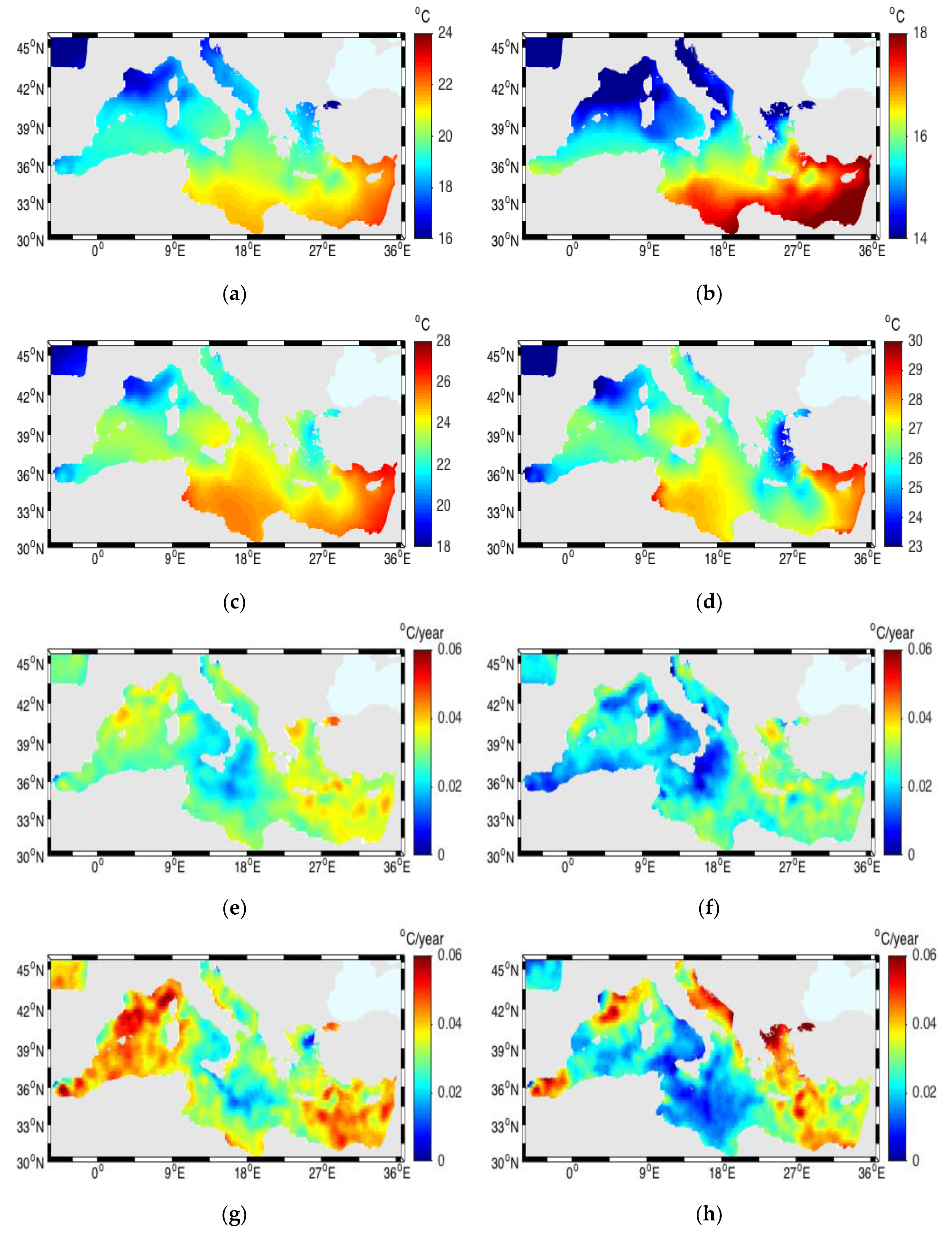
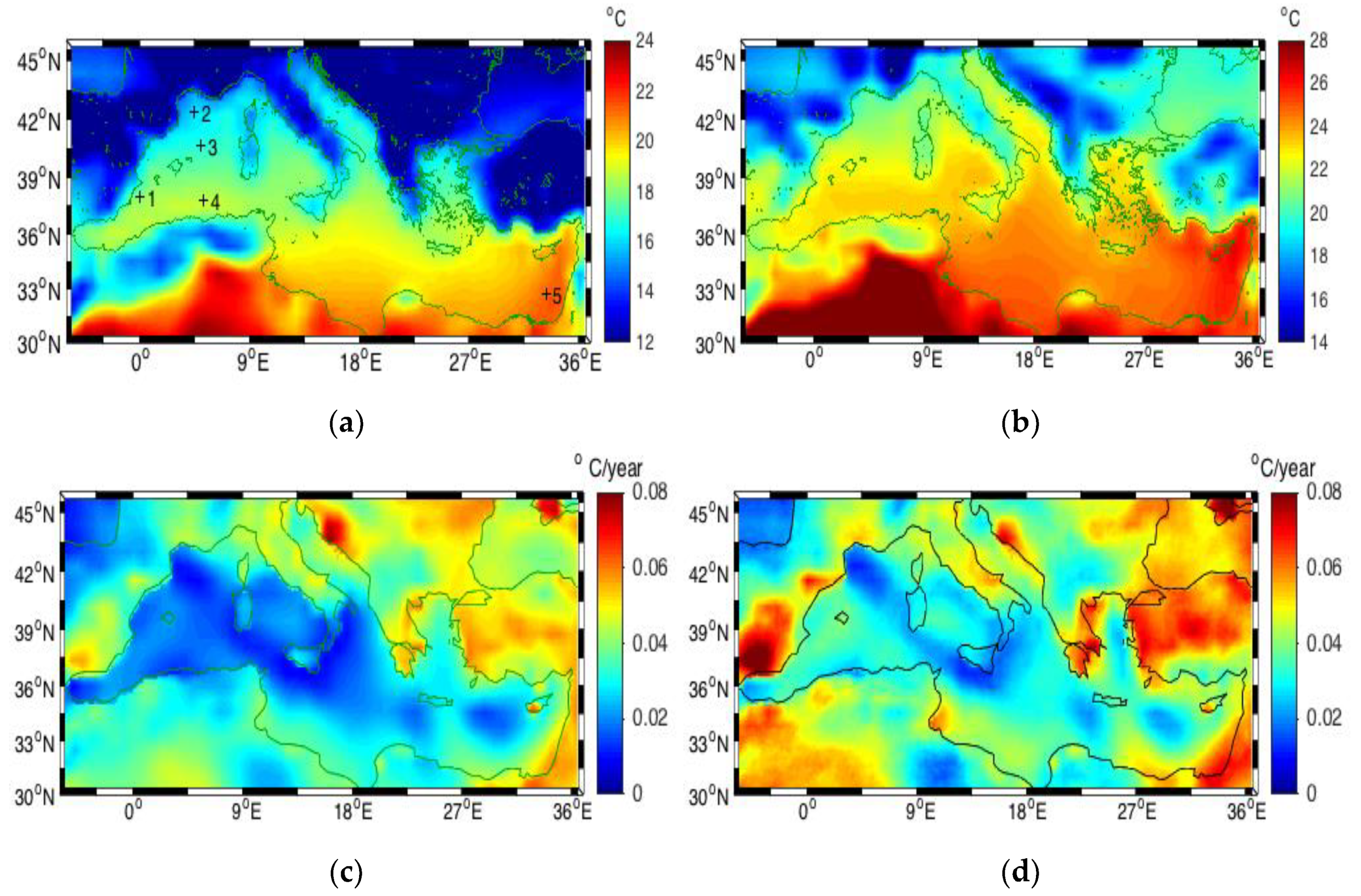
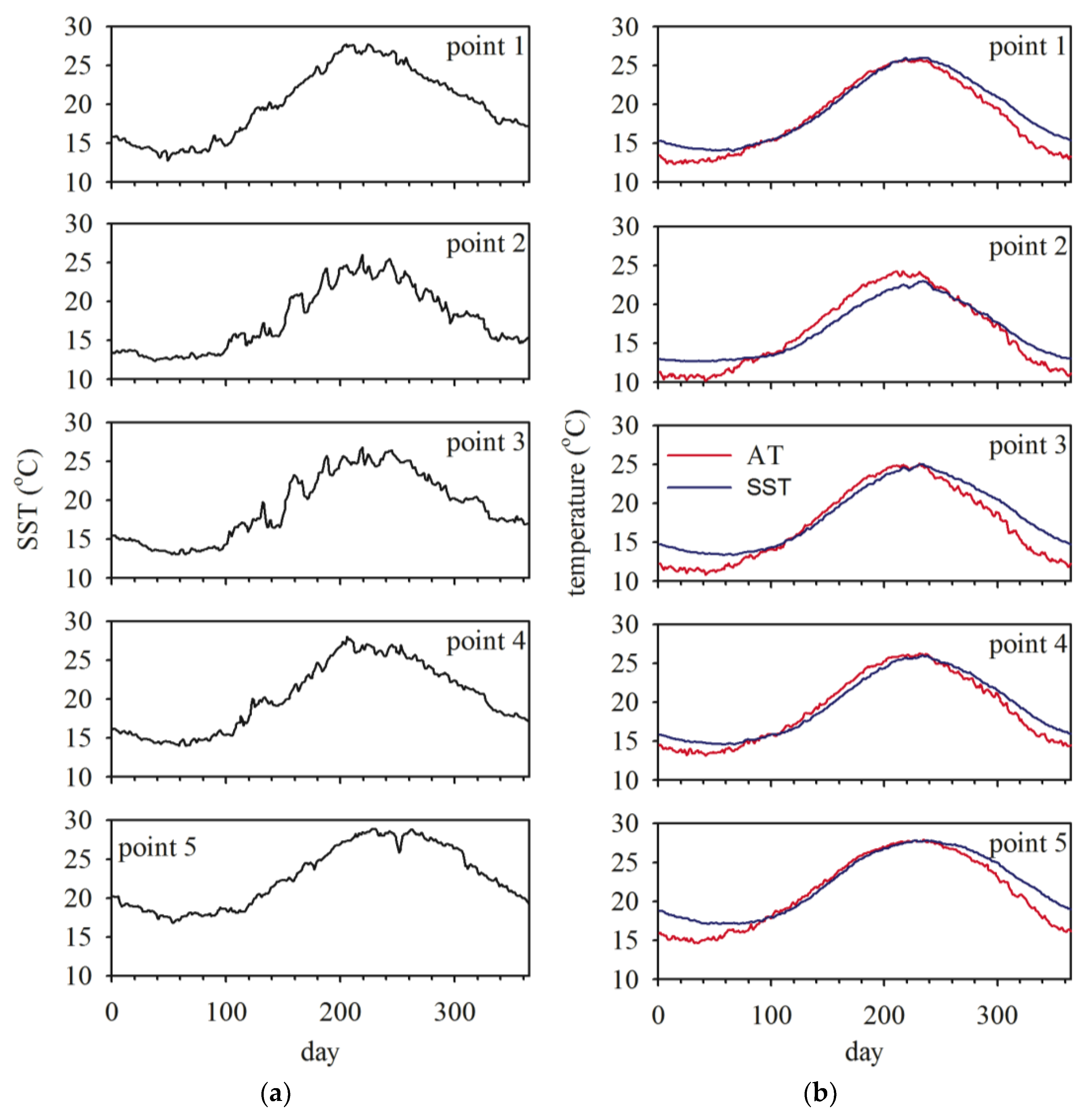
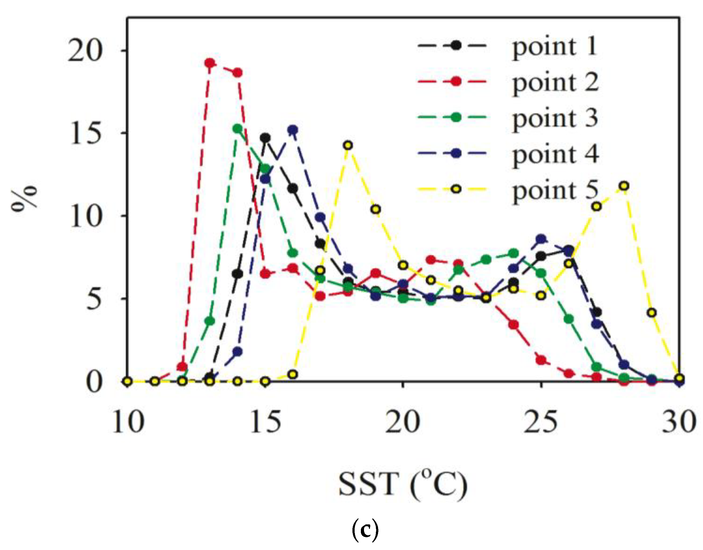
3.1. Sea Surface Temperature (SST)

In this section we briefly characterize the spatial distribution of SST and its variability. Figure 2a shows SST averaged in the entire 1983–2017 time interval. The average SST increases generally from north to south over most of the Mediterranean Sea, except over the northern Tyrrhenian and the Levantine sub-basins, where it increases from west to east, likely due to the Mediterranean surface circulation. The highest temperatures are found in the south-eastern Mediterranean, while the lowest are observed near the north-western coast and in the Adriatic Sea. Patterns in spatial distribution of the mean annual 25th, 75th and 98th percentiles (Figure 2b–d) look similar, although their values are different. The percentiles were calculated for each year and its values were averaged in the 36-year time interval. The lowest values of 25th percentiles are about 14 °C (northern part of the MEDIT). The lowest 75th percentiles (22–23 °C) are located near the Gulf of Lion, the Alboran Sea and in the vicinity of the Strait of Gibraltar, as well as in the Aegean Sea. The highest values of the 75th (about 27 °C) and 98th percentiles (>28 °C) are present in the southern part of the Ionian Sea and the Levantine basin. Spatial distribution of SST is influenced by the air-sea interaction processes and by water circulation patterns. This can be observed if one compares Figure 2 with atmospheric data discussed in the next section.

Time series of annually averaged SST data were used to estimate regional SST trends presented in Figure 2e. SST trends presented here are statistically significant at 95% confidence level, p < 0.05. Trends of increasing annual mean SST were detected over the entire Mediterranean Sea. Trends are ranging from about 0.02 °C yr⁻¹ (in the mid-western Ionian sub-basin) to about 0.045 °C yr⁻¹ (north-east of the Levantine sub-basin). For comparison, the globally averaged SST trend calculated using 20 years of Advanced Very High Resolution Radiometer Pathfinder data (January 1985 to December 2004) was estimated as 0.018 °C and 0.017 °C yr⁻¹ from daytime and night-time data, respectively [34]. The warming trends estimated by us for the MEDIT Sea are greater than these global estimates. Trends for the annual median SST values (not shown) are almost identical as trends for the annual means. Trends for the 25th percentiles are lower than trends for the means (Figure 2f). However, trends for the 75th percentiles are higher than trends for the 25th percentiles, means and medians with the highest values reaching 0.06 °C yr⁻¹ in the western part of the MEDIT (where annual mean SST values are low) and in the south-eastern part of the sea (where annual mean SST values are high). This indicates that the mean SST in the MEDIT increases mainly due to changes occurring in the warmer seasons of the year. This conclusion is also supported by trends based on the monthly SST data [16,17]. Note that the 98th percentiles reach the highest values in the south-eastern part of the MEDIT (Figure 2d) and spatial pattern of their trends (Figure 2h) is somewhat different than it was the case with trends for the 75th percentiles. The strongest trends for the 98th percentiles are noted in the belt extending from the Aegean Sea into the Levantine Basin, in the Adriatic and Alboran Seas and in the vicinity of the Gulf of Lion. For comparison, based on data from 1985–2006 it was found that SST trends are different in the western (0.03 °C yr⁻¹) and eastern (0.05 °C yr⁻¹) part of the Mediterranean [35]. Warming trend averaged for the entire Mediterranean basin was estimated as 0.036 °C yr⁻¹ [17].

Overall variability of SST in the MEDIT is characterized by a well-pronounced seasonal cycle. This is summarized in Figure 3. The annual maximum temperatures averaged in the 36-year time interval vary between 24 °C in the northern part of the MEDIT (Alboran and Aegean Seas) to 28 °C in the warmer southern part of the MEDIT. The maximum SST (displayed in Figure 3c) during the entire time interval considered (1982–2017), ranged between 26–31 °C. The maximum SST had the lowest values in the Gulf of Lion, the vicinity of the Strait of Gibraltar and in the Aegean Sea. The 36-year average annual minimum SST and the minimum SST observed during the entire observational time interval (1982–2017) are shown in Figure 3b,d, respectively. Temperatures as low as 8 °C are seen near the northern coasts of the MEDIT. As far as the phase of the annual SST cycle is concerned, the maximum SSTs occur around days 225–240 (July–August), while the minimum temperatures are detected around days 30–80 of the year (February–March, see Figure 3e,f). The 36-year averaged amplitude of the annual cycle (Figure 3g) varies between 10–13.5 °C, with the smallest values noticed in the south-eastern part of the MEDIT (where SST values are consistently high) and in the Gulf of Lion, Alboran and Aegean Seas (where SST values are low). Annual amplitudes have been calculated as the difference between the maximum and the minimum SST values in each year and then the 36-year averaged amplitude was estimated.

Apart from the long-term trends and annual cycle, variability of SST can be observed on a synoptic scale and can be characterized by standard deviation (STD) of SST anomalies. The anomalies are calculated by subtracting the average annual cycle and the long-term trend from daily SST data. Spatial patterns of STD are exhibited in Figure 3h. As can be seen, STD values are greater in the northern part of the MEDIT than in the southern part. This can be explained by the fact that larger STD values are associated with regions more influenced by strong winds (discussed later) causing intermittent upwelling and variability in the water circulation and advection patterns. High water temperature is considered in the literature [36,37,38] as one of the most important factors limiting the growth of P. oceanica meadows but there is a lack of research documenting in detail how this seagrass responds to different scales of variability and what would be the temperature threshold levels for strong negative impacts. Nevertheless, a complete description of thermal conditions experienced by P. oceanica in different regions of the MEDIT can help to elucidate these relationships in the future.

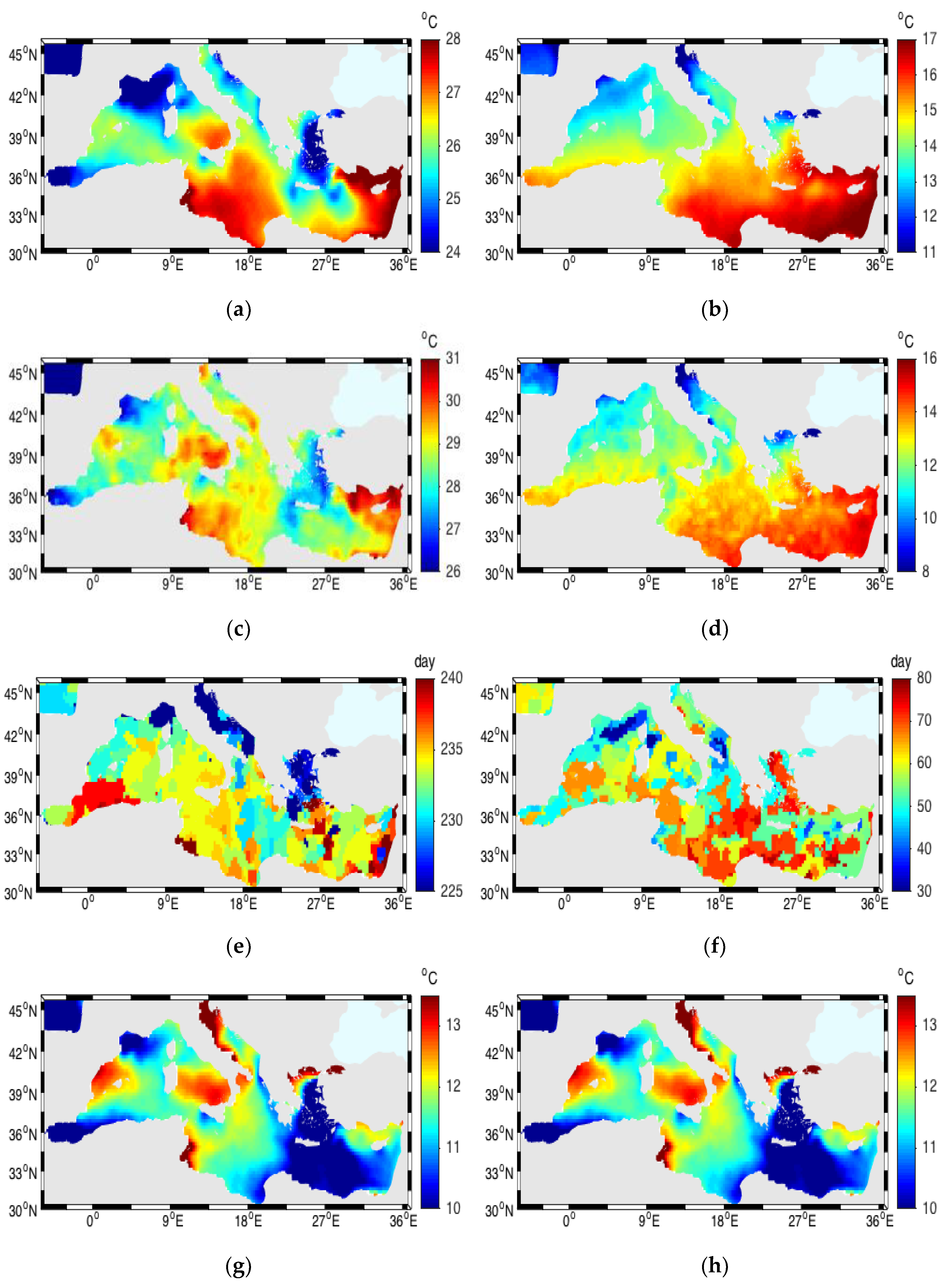
3.2. Air Temperature

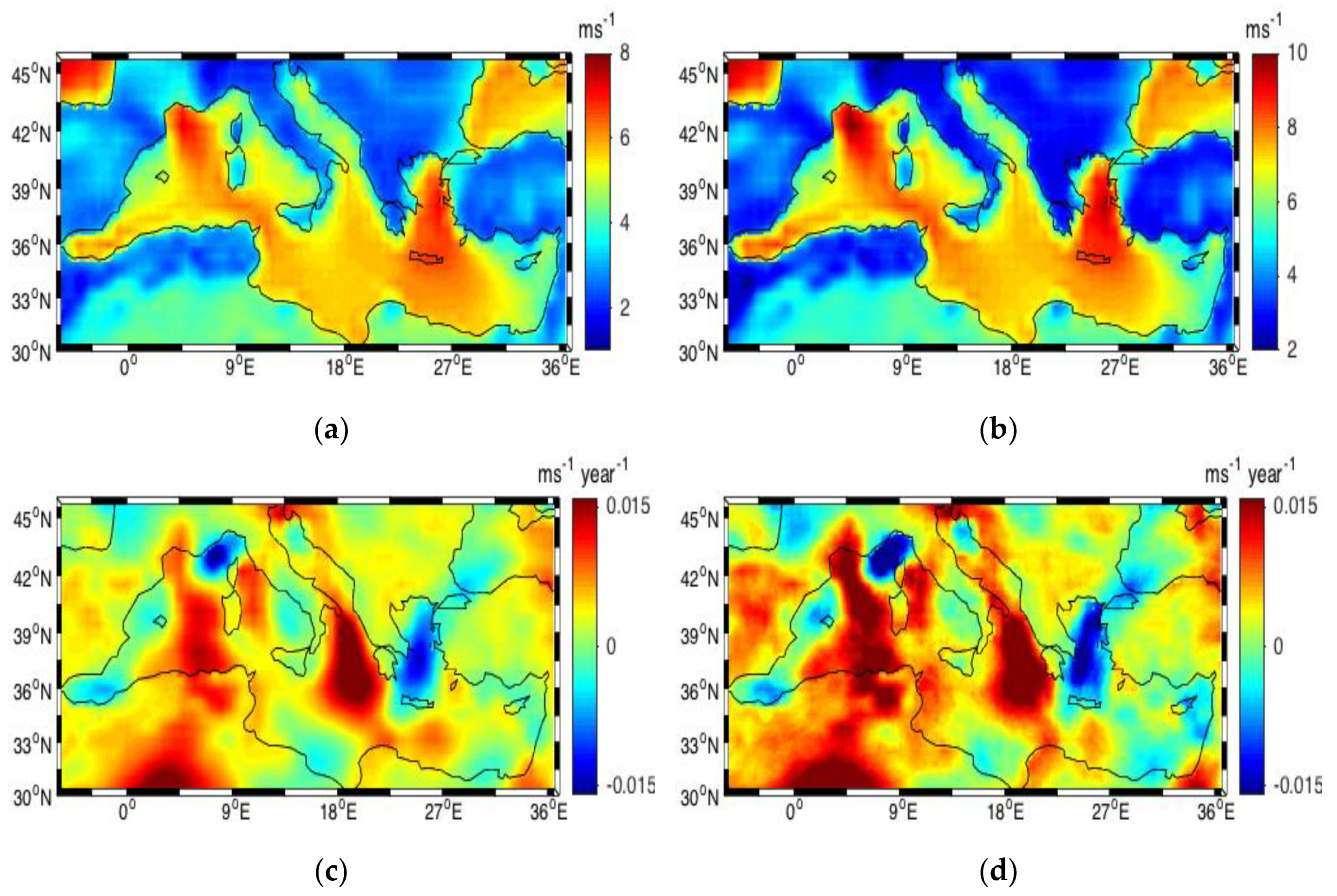
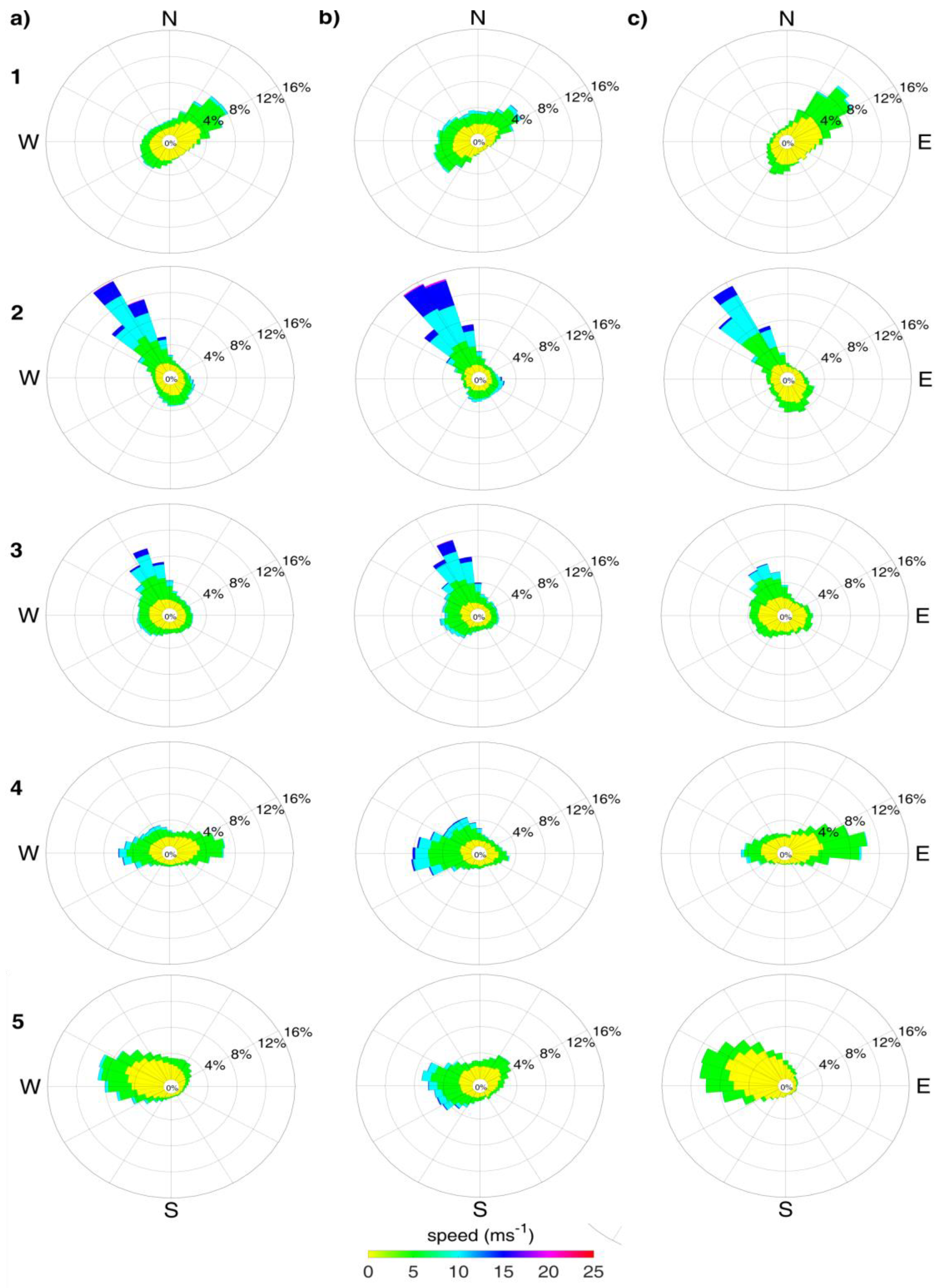
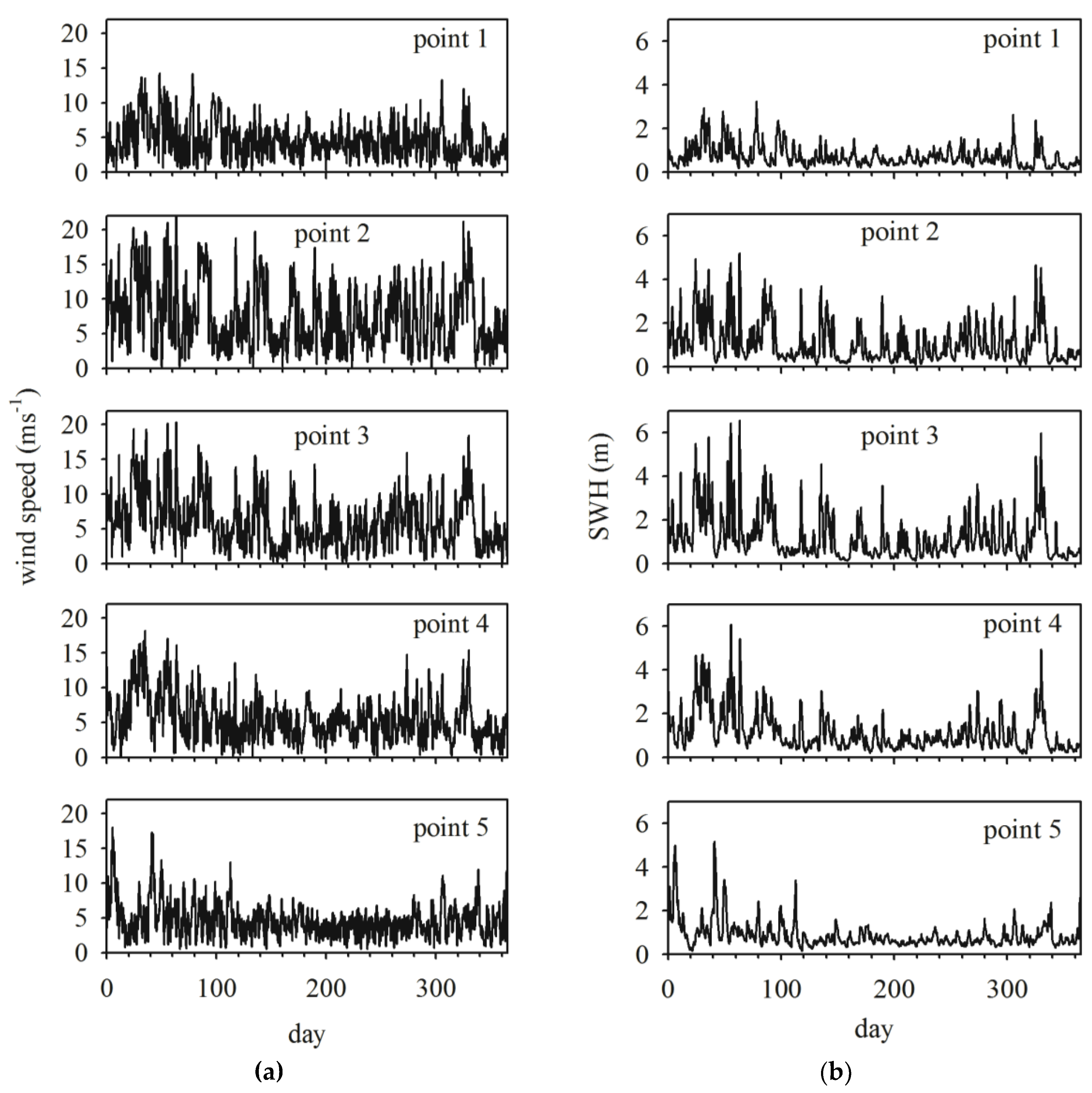
In this section the spatial distribution of air temperatures (AT) and its variability is briefly summarized. Although we do not expect air temperature to directly affect seagrass distribution in the MEDIT, the AT and its relation to SST is an important indicator of air-sea interaction processes. The 36-year averaged mean AT and annual 75th percentile averaged over the 36 years are displayed in Figure 4a,b. We can see that the most obvious spatial patterns in AT over the MEDIT are quite similar to the spatial patterns in SST. By this we mean that there is a well pronounced gradient of AT between the northern and southern parts of the MEDIT. In addition, the highest AT values are present in the southern part of the Ionian Sea and the Levantine basin, the same regions where we noted the highest SST values. High AT values are associated with the land of North Africa. Long-term trends in the annual mean AT and 75th percentiles (Figure 4c,d) are larger above the land than above the sea surface. They are statistically significant at 95% confidence level, p < 0.05. Trends for the 75th percentiles are higher than trends for the mean ATs, in particular in the western part of the region (Spain and north Africa), where they reach in some locations as high values as of 0.08 °C yr⁻¹.

To better relate the seasonal cycle of SST and AT we have extracted time series data in the 5 example locations (points) indicated in Figure 4a by crosses. Location 1 represents the site near the Alicante (Spain), location 2 is in the Gulf of Lion (France), location 3 in the open sea near the Balearic Islands, location 4 near the coast of North Africa and location 5 is in the south-eastern part of the MEDIT region (the warmest region). Note, that the exact geographical position of selected pixels is not important here, we merely wanted to show the differences in the temporal patterns of variability using few points representing different regions of the MEDIT. Time series of AT and SST in selected 5 locations are compared in Figure 5. On the left side of Figure 5 (panel a) we can compare time series of SST values for year 2015. The presented data show that there is a lot of variability on a synoptic time scale, in particular at location 2 and 3. Figure 5b compares annual cycle of AT and SST using the 36-years averaged daily data. As we can see, the lowest SST and AT values are associated with the Gulf of Lion (point 2). At all 5 locations ATs are lower than the SSTs in the fall and winter seasons. This tendency starts around 230–250 day of the year. The biggest difference between AT and SST in the summer is observed in the Gulf of Lion. In the spring, on average around day 80–100, ATs become larger than SSTs. Note also that the highest frequency of occurrence of high SST values (>25 °C) in the entire investigated time interval (36 years) was observed in point 5 (Figure 5c).

3.3. Winds

Long-term wind speed and direction time series are important for understanding of the regional climate change. Winds influence the rate of exchange of heat between the atmosphere and the ocean, as well as the evaporation. Wind-driven circulation, wave field and storm surges affect coastal processes and can be of importance for explaining some spatial patterns in seagrass distribution. ERA Interim reanalysis data used in our paper are based on wind data from remotely operating instruments such as radar altimeters, scatterometers, passive microwave radiometers and synthetic aperture radars assimilated to a numerical model [18].

Figure 6a,b illustrate spatial distribution of the 36-year averaged annual mean and the 75th percentile wind speed. The windiest areas of the Mediterranean Sea are the Gulf of Lion and a belt extending from here to the E. Algerian Basin, as well as the area surrounding the longitudinal axis of the Aegean Sea and the S Levantine Basin. Various geomorphological and topographical features and complex coastlines and local orography significantly influence the wind patterns in the MEDIT, both spatially and temporally (see Figure 1). Regional wind patterns include the mistral and the tramontane [39,40]. Mistral, the cold and dry north-northwest wind, blows in the Gulf of Lion, occasionally up to the African coasts. When it enters the Tyrrhenian Sea, the mistral is characterized by a more pronounced southward direction and is named maestrale. The central Mediterranean is influenced (especially in winter) by the westerly to south-westerly libeccio and by the wet and warm sirocco. Sirocco in autumn can blow from south to east, producing the storm surges flooding the Venice Lagoon. The bora, classified as an orographic or downslope wind, is a north-easterly strong and cold wind affecting the entire Adriatic Sea [41]. Bora-type winds exist also in other regions, as in the northern Aegean Sea where north-easterly winds are frequent. In the Levantine Basin the prevalent winds are the etesians [42]. These winds are particularly strong in the summer. In the Alboran Sea, the west-southwest vendaval occurs mainly from October to November and from February to March, when it can be very strong. The easterly levanter blows in all seasons but in winter it may be strong and long lasting (up to 10 days). For a detailed description of the main Mediterranean wind patterns see [43] and references therein. The Mediterranean Sea is one of the most cyclogenetic areas in the world with explosive cyclogenesis and tropical-like cyclones [44,45,46,47].

The spatial distribution of trends in wind speed is depicted in Figure 6c,d. Orange/red and deep blue colours represent the areas where statistically significant trends were found. Statistically significant positive trends in the annual mean and the 75th percentiles of wind speed have been detected in two regions extending from the north to the south. The first region starts in the Gulf of Lion and the second region in the Adriatic Sea. The strongest positive trends are observed in the Ionian and Adriatic Seas, the eastern part of the Algerian Basin up to the Balearic Islands and the Gulf of Lion. The negative trend is observed offshore the coasts of Monaco in the Ligurian Sea and in the central Aegean Sea. These results are in qualitative agreement with previous studies [48] although the spatial and temporal extents of the analysed datasets were somewhat different.

To highlight the regional differences in the variability of winds, we have plotted in Figure 7 example wind roses for selected 5 locations displayed in Figure 4a. Data are presented for the full 36-year long time series (column on the left side) and for the winter (January-February, middle column) and the summer seasons (June-July, column on the right side). Our results confirm that seasonal variability can be significant, depending on location. Regarding long-term trends in wind direction, comparing data from the first 10-years (1982–1991) and the last 10 years (2008–2017) of the time interval analysed here, we observed that the main patterns in wind direction over the MEDIT did not change significantly (not shown).

Winds have an indirect influence on other environmental conditions directly affecting seagrasses. Winds control surface wave propagation patterns and sea state. Moreover, the spatial distribution of sea surface temperature and sea level rise may be also affected by wind patterns. Strong and persistent winds may favour the upwelling of deep cold water masses to the surface. For example, the presence of the cold SST in the northern Adriatic Sea can be explained by the influence of the bora winds. The Aegean Sea SST is low due to the impact of cold and dry etesian winds. The Gulf of Lion is characterized by the much colder SST than the rest of the Mediterranean Sea, mainly as a consequence of the mistral winds.

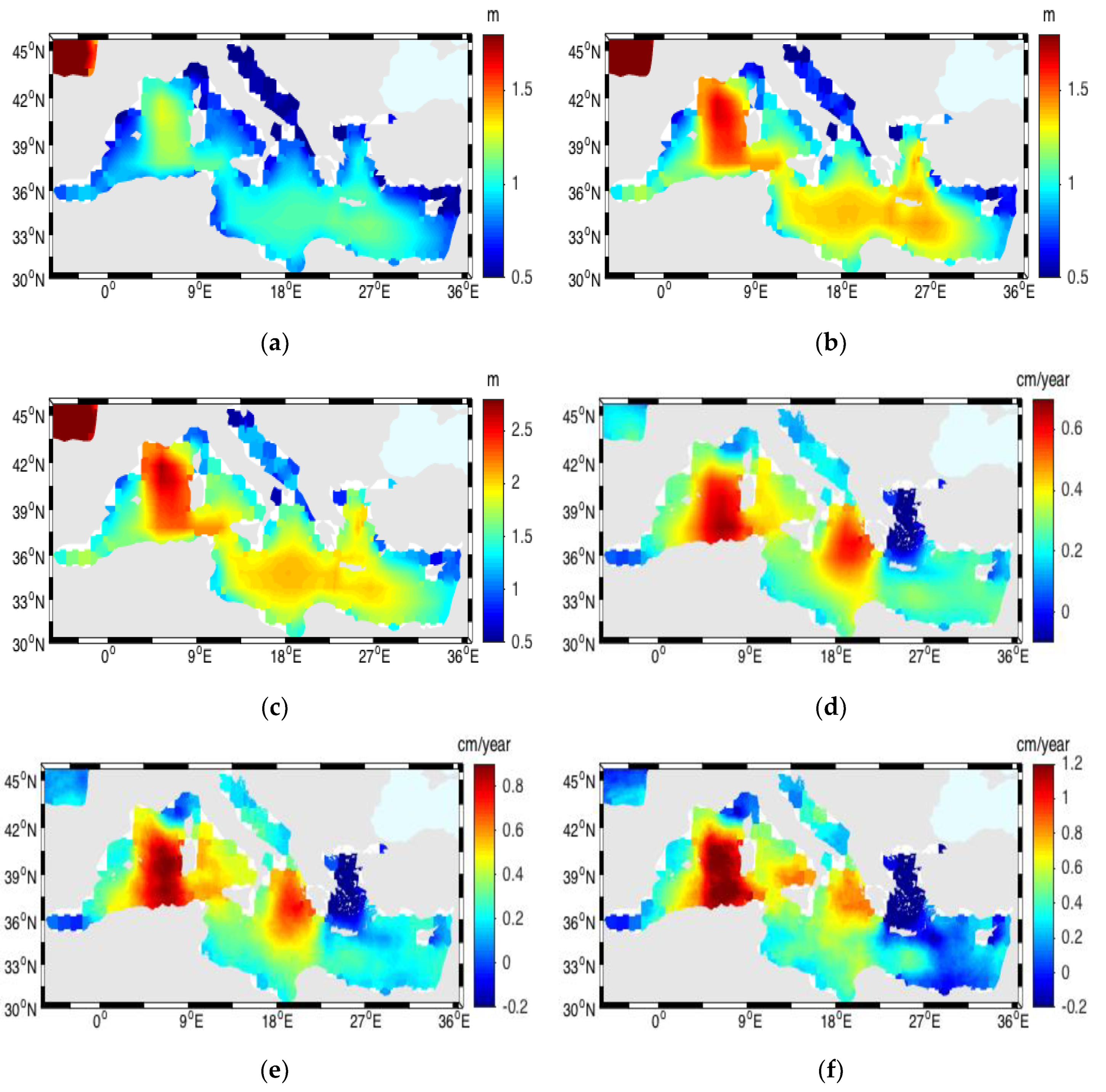
3.4. Significant Wave Height

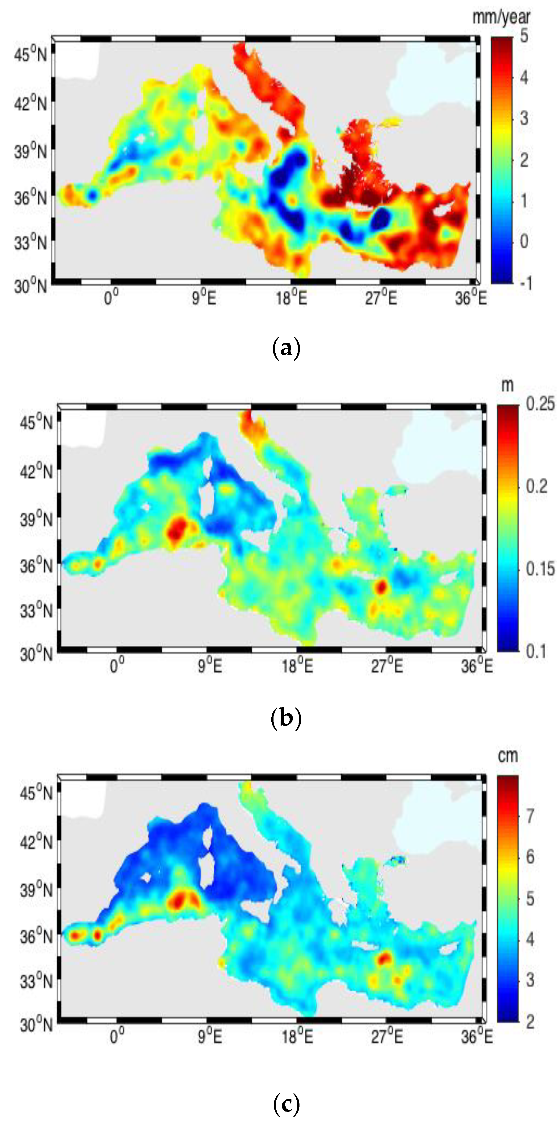
The height of significant waves is strongly dependent on wind force, duration and fetch. The spatial distribution of significant wave height (SWH) averaged over the time interval 1982–2017 and the mean annual 75th and 90th percentiles (percentiles estimated using the annual time series and averaged), are displayed in Figure 8a–c, respectively. The mean SWH in the MEDIT is smaller than in the open Atlantic Ocean and is below 1.2 m even in the region where it reaches the largest height. The 75th and 90th percentiles achieve 2 and 2.5 m respectively, with the greatest values in the region extending from the Gulf of Lion in the southward direction. This is the region where high wind speed is often observed (due to the presence of the mistral) as was shown in Figure 6. Fairly large 75th and 90th SWH percentiles are also detected in the open waters of the southern part of the MEDIT. Multiyear trends in SWH (Figure 8d–f) are characterized by patchy spatial distribution with the highest positive values in the same regions where the largest positive trends in wind speed have been documented (compare with Figure 6). Positive trends reach the greatest values for the 90th percentiles (1.25 cm/year) in the region extending from the Gulf of Lion in the southward direction. This indicates that the largest waves are becoming more frequent there. Negative SWH trends are observed offshore the coasts of Monaco, in the Ligurian Sea and in the Aegean Sea. These are the regions were negative trend in wind speed have been noted (Figure 6).

It is difficult to compare our results with other authors, since previous research was focused on different time intervals. For example, the variability of the monthly average significant wave height (SWH) in the Mediterranean Sea in years 1958–2001 is described in Reference [49]. The authors concluded that the annual cycle consists of two main seasons, winter and summer. Eastwards and south-eastwards propagating waves prevail in the winter all over the basin. The summer is characterized by the southwards propagating waves in the Aegean Sea and Levantin Basin. The spring and the fall are transitional time intervals with northwards and north-eastwards propagating waves, associated with an intense meridional atmospheric forcing [49]. Thus, the spatial patterns of waves in the Mediterranean are strongly influenced by the wind speed and fetch, dependent on the regional orographic features. Surface atmospheric circulation events with larger fetch are more effective in producing higher waves. Large inter-annual and inter-decadal variability of SWH field was described and a statistically significant decreasing trend of mean winter SWH values was implied in Reference [49]. This trend was calculated based on SWH averaged over the entire basin. However, using more recent data (1979–2013) it was argued that after a general decrease of the mean yearly wave power in the 80’s and 90’s, there was a positive trend in the time interval 2005–2013 [50]. Our results show that SWH trends are characterized by a significant spatial variability and assume positive and negative values depending on the location. This may explain why the previous studies, where spatial distribution and variability SWH was not fully analysed, did not detect positive SWH trends.

To better illustrate the local and seasonal variability of SWH and its association with wind speed we plotted in Figure 9a,b time series of wind speed and SWH in 2015 in 5 locations (points) marked in Figure 4a. As expected, larger SWH are generally associated with stronger winds. Data for location 2 underline the importance of wind fetch. At this location the wind fetch is limited, as strong winds usually blow from the coast. Figure 9c compares the frequency distribution of SWH at each point, based on full 36-year long time series. Larger SWH are more often observed at location 3 (near Balearic Islands) than at location 2, because at location 3 fetch for strong winds is larger. Large SWH (~2 m and more) are the least frequently observed at location 1, where wind speed does not reach very high values and wind fetch is often relatively small. Note that at points 2, 3, 4 there is on average few days per year when SWH is 4 m or more.

3.5. Sea Level

Satellite altimetry data were used to estimate local sea level variability summarized in Figure 10a–c. Our results indicate that there is a consistent, statistically significant (95%, p < 0.05) trend in sea level anomalies (SLA) in the major part of the MEDIT. Trend is spatially variable with the largest positive values (~5 mm yr⁻¹) in the eastern part of the sea. Negative trend (−2 mm yr⁻¹) was detected in the central part of the MEDIT. For comparison, the rate of globally averaged sea level rise is 3.1 mm yr⁻¹ (or 3.4 mm yr⁻¹ if the correction for global isostatic adjustment is taken into account) [51]. Thus, sea level trend in the eastern part of the MEDIT is greater than the globally averaged trend derived from satellite altimetry data. Figure 10b shows the spatial distribution of the mean annual 99th percentile of SLA. The largest 99th percentiles are observed near the northern coast of Africa, a region located in the southern edge of the belt of high wind speed, extending south from the Gulf of Lion. Large 99th percentiles are also seen in the northern Adriatic Sea, where storm surges flooding the Venice Lagoon are a well-known problem. Figure 10c presents spatial distribution of the standard deviations (STD) of SLA, after the long-term trend has been removed. Data shown in Figure 10c indicate that on average, sea level is the most variable in the southern part of the MEDIT in the same locations where we observed the largest 90th percentile SWH. Another region where the 99th percentiles and the STD reach relatively high values is located in the central part of the southern MEDIT.

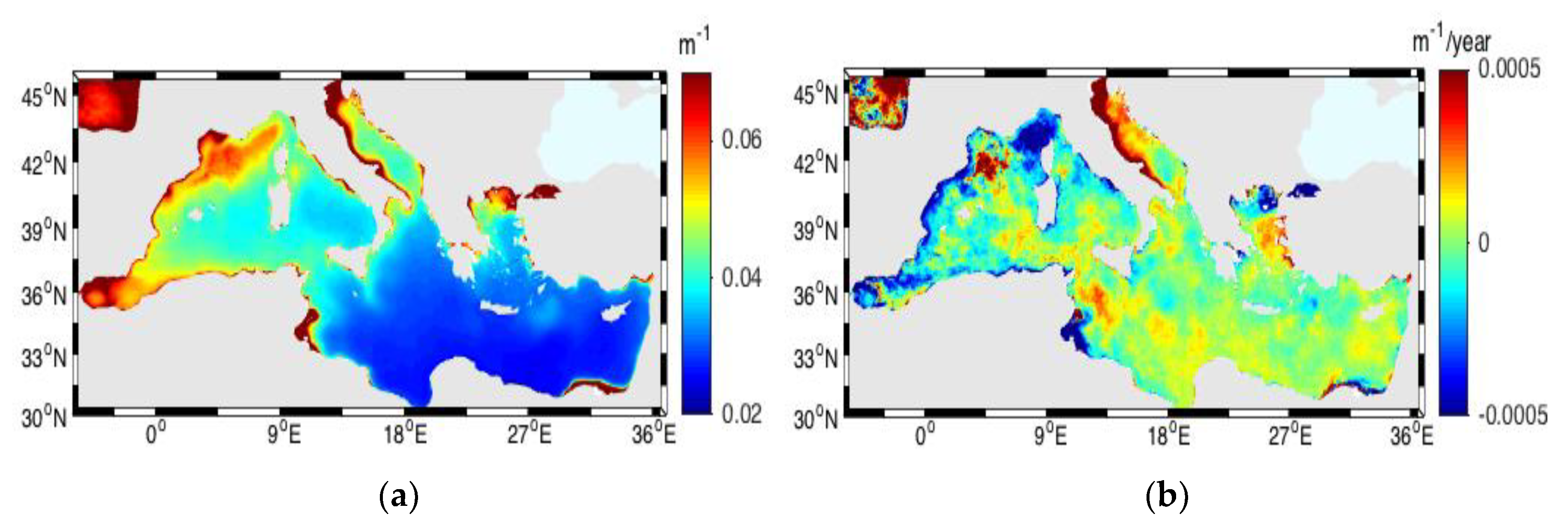
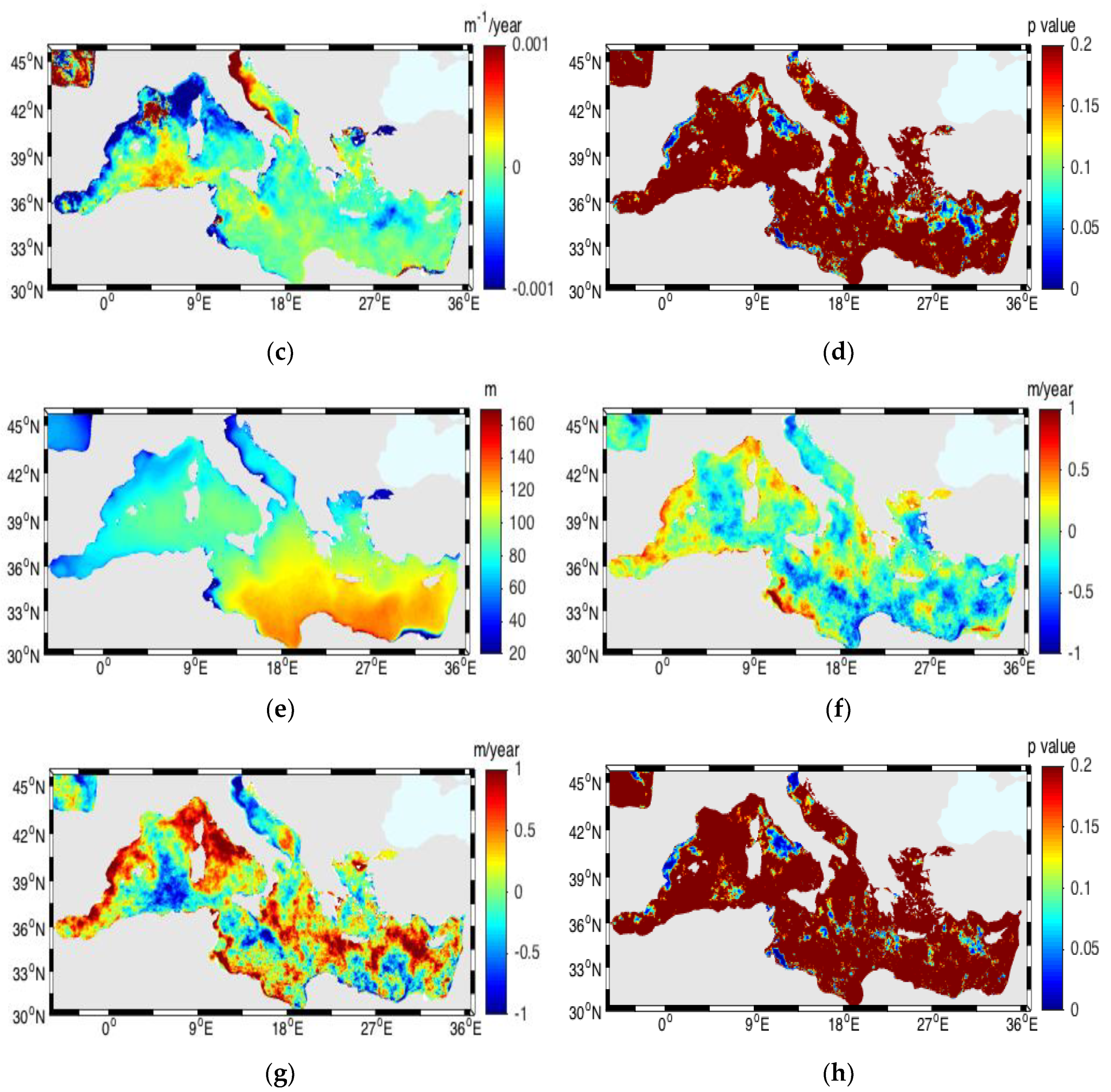
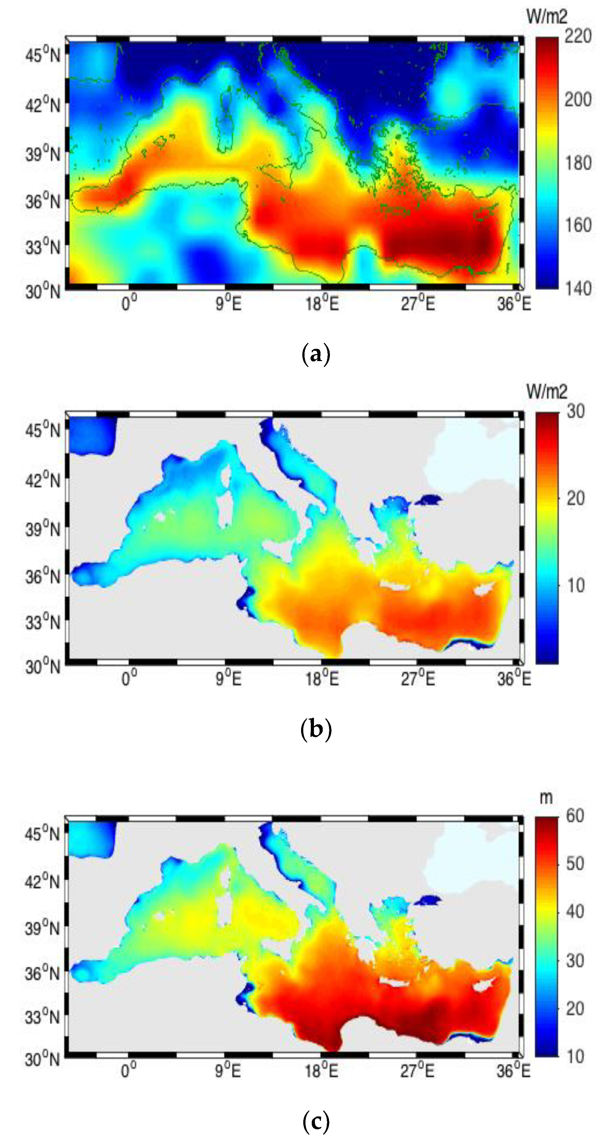
3.6. Vertical Diffuse Attenuation Coefficient and Euphotic Depth

In this section, we summarize the main results from the analysis of ocean colour remote sensing data, relevant to our research. We focus on the vertical diffuse attenuation coefficient K_d(490) and the euphotic depth Z_eu data.

It must be mentioned that the Mediterranean Sea has somewhat unusual optical properties of the water, which have been described in the literature as “oligotrophic waters less blue and greener than the global ocean” [52]. Several hypotheses were developed in the past to explain these optical properties. One hypothesis draws attention to relatively high concentrations of coloured dissolved organic matter, responsible for the enhancement of water absorbing properties [53,54]. Second hypothesis points out to a reinforcement of scattering due to the presence of coccoliths [55], while yet another one emphasizes the role of submicron Saharan dust in suspension in the surface waters [56]. These aspects are important if one wants to derive quantitative estimates of concentration of chlorophyll (or other water component) from ocean colour but they are not as crucial if one is simply interested in the euphotic depth and attenuation of light in the water column. K_d(490) and Z_eu are cumulatively influenced by all the optically significant water components and we are at this moment not concerned with what is the relative importance of each of the components.

Figure 11 presents the spatial distribution of the climatology of the vertical diffuse attenuation coefficient K_d(490) and the euphotic depth Z_eu, based on ocean colour data from MODIS-Aqua. Smaller values of K_d(490) and deeper Z_eu are associated with oligotrophic waters and are observed in the southern part of the MEDIT. This is a region were high SST values have been noted in Figure 2 and Figure 3. Shallower Z_eu and larger K_d(490) values are observed in the north-western part of the MEDIT. Spatial distribution of K_d(490) in Figure 11 is consistent with a general picture of the Mediterranean Sea characterized by the existence of significant west-east and north–south gradients in in situ bio-optical observations [57] and ocean colour data [58,59,60,61,62]. Coastal regions associated with high concentrations of coloured dissolved organic matter and terrigenous mineral particles are also visible in Figure 11. An example is the north Adriatic Sea where high K_d(490) values can be linked to the presence of big rivers, such as the Po, Brenta, Livenza, Adige and Isonzo. Every year rivers bring substantial quantities of terrigenous organic and mineral particles as well as dissolved organic matter and release large amounts of nutrients that support the micro-phytoplankton growth in coastal waters. All these substances have significant impact on water optical properties, as a result high values of K_d(490) are observed in this region.

Trends in K_d(490) and Z_eu are displayed in Figure 11b,c,f,g. Our results show a rather complex pattern of both negative and positive trends in K_d(490) and Z_eu. Note that ocean colour data series used for these calculations are rather short (15 years), therefore our findings need to be taken with caution. Considering only those areas where trends are statistically significant (Figure 11d,h), we notice an evident negative trend in K_d(490) (positive trend in Z_eu) along the coasts of Spain (i.e., off the Costa Blanca, South-East Spain) and in the Ligurian–Provençal basin. A positive trend in K_d(490) (negative trend in Z_eu) is detected in the North Adriatic Sea and in the oligotrophic southern part of the MEDIT. Note however, that since data series are so short, the detected trends are not statistically significant in most areas of the MEDIT. The seasonal cycles of K_d(490) and Z_eu in the MEDIT (not shown) follow the life cycle of the phytoplanktonic organisms, the typical pattern of temperate areas with a biomass increase in late winter/early spring, followed by a decrease of biomass during the summertime and a second smaller bloom in the autumn. Similarly to Chl concentration (not shown), K_d(490) also displays highest values in the spring, therefore we here present also trends for spring (March-May averages, Figure 11c,g). Our results suggest that although light limitation may be a problem for P. oceanica meadows in the Adriatic and along the north-western coast of the MEDIT, the euphotic depth has positive temporal trend (K_d(490) is decreasing) along the Spanish coast, indicating that the conditions for P. oceanica are improving there. This is not the case in the north Adriatic Sea, where the conditions are worsening, as the euphotic depth there is decreasing (K_d(490) is increasing).

It is hard to compare our results with other data from the literature. For example, Chl trends based on 1998–2009 SeaWiFS data from the summer season [63] were not statistically significant in almost half of the Mediterranean Sea. Statistically significant negative trends were found in offshore waters of the north-western MEDIT. In the western coast of Greece, as well as in a narrow belt along Egyptian, Tunisian, Maltese and Turkish coastlines Chl trends were positive. When ocean colour Chl data from the same time interval were analysed using a different approach (Chl was derived using regional algorithms and trends were estimated after application of the seasonal adjustment methodology), positive trends around the Balearic Islands, in the Ligurian–Provençal basin, in the Rhodes Gyre region and off the Nile River delta were discovered [64]. Trends were negative in the North Adriatic Sea and near the Rhone River mouth. Note that these results cannot be directly compared with our results, because we have analysed different quantities (K_d(490) and Z_eu) and used longer time series covering time interval (2003–2017). In addition, we must stress again that a rigorous analysis of climate related trends requires longer data sets than are currently available from ocean colour satellite sensing.

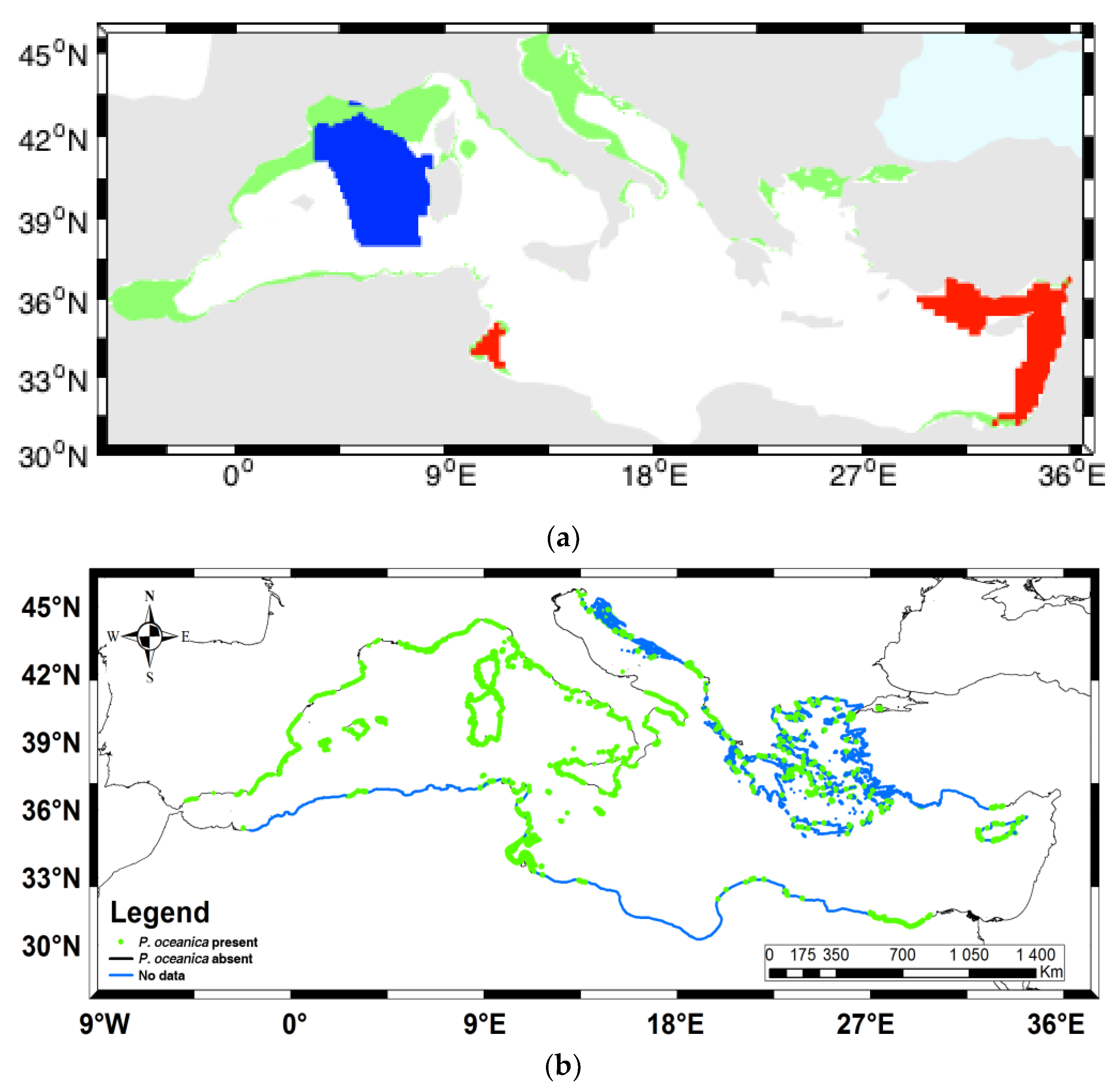
4. Discussion of Potential Influences of Environmental Conditions on Posidonia oceanica

In this section we will briefly summarize what is known from the literature about how the environmental conditions influence P. oceanica growth and distribution, and compare it with our results. The basic requirements for seagrass survival are analogous to requirements of all plants [64]. Thus, the main environmental factors influencing the growth of P. oceanica are availability of nutrients, inorganic carbon and light for photosynthesis, as well as water temperature [28]. The exposure to significant mechanical disturbances, for example waves and currents, can destroy the meadows.

Water temperature affects all biological processes, primarily by increasing reaction rates of the biochemical pathways [28]. Thus, photosynthesis and respiration are slower at low temperatures and increase with increasing temperature. Thermal optima associated with high rates of photosynthesis range from approximately 15 to 33 °C [65,66]. Seagrasses can be affected by thermal stress in a number of ways. Because the increase in carbon uptake (photosynthesis) with temperature is slower than the increase in carbon consumption (respiration), at high temperatures the respiration can exceed photosynthesis, resulting in a negative energy balance within the plant [67]. What is more, quick reduction in photosynthetic efficiency takes place after temperature exceeds the optimum threshold [68]. Complete data documenting all the details of the responses of P. oceanica to temperature are unavailable. Optimal temperatures for growth are believed to be around 15.5 to 18 °C [69]. The optimal temperature for photosynthesis is higher. In situ experiments revealed that P. oceanica meadows show negative responses to warming above 27 °C, when increased shoot mortality was observed [36]. Laboratory experiment showed a negative reaction of P. oceanica seedlings to warmer temperatures with reduced growth rates, leaf formation rates and leaf biomass per shoot [37]. Another laboratory study demonstrated that newly germinated seedlings of P. oceanica are vulnerable to the extreme temperature events [38]. Temperatures above 27 °C significantly affected the photosynthetic rate of the seedlings, decreasing the production of oxygen and the performance of the PSII. One-month exposure of the seedlings to temperatures above 29 °C produced negative shifts in their development, especially in leaf growth and mortality. Summarizing, water temperature can define the geographical limit for growth of P. oceanica, although it is possible that some adaptation mechanisms to changes in local temperature regimes exist.

Another important factor controlling seagrass spatial distribution is light. Availability of light is a fundamental requirement, since light is necessary for photosynthesis [28]. In the aquatic environment light is a limited resource. Irradiance reaching the sea surface is in the water column strongly absorbed and scattered by pure water and its optically active components (phytoplankton, other suspended material and dissolved substances). As a result irradiance is attenuated exponentially with depth and its spectral composition changes [27,28]. Vertical diffuse attenuation of underwater irradiance (K_d) varies spatially and in time, since it depends on concentrations and quality of water components. As a rule of thumb it is assumed that P. oceanica needs approximately at least 10% of the surface irradiance in order to grow [65]. This requirement confines seagrass to shallow coastal waters (to about 45 m, depending on water clarity). Morphological acclimatization to reduced irradiances at depth in growth strategy of P. oceanica includes reduced shoot density in deep waters. Better knowledge of light requirements for seagrass growth could help with predictions of the lower depth limits for seagrass.

In addition to light, seagrasses need inorganic carbon and nutrients. The actual importance of carbon limitation to seagrass photosynthesis and growth is not well known and needs to be examined further [65]. Nutrient requirements for seagrasses are lower than for macro algae and phytoplankton [70]. It has been estimated that seagrasses need about 4 times less nitrogen and phosphorous per weight than phytoplankton. This makes an advantage for seagrass growth in nutrient-poor environments. It is also advantageous that seagrasses can additionally take up nutrients from sediments, which usually are rich in nutrients due to the mineralization of organic matter. Seagrasses also require oxygen to supply their metabolism of both above- and below-ground tissue [65]. Leaves are usually situated in the oxygenated water column but roots and rhizomes are buried in anoxic sediments. Under normal circumstances, oxygen is transported to roots and rhizomes by diffusion from the leaves through a well-developed system of air tubes (lacunae) running through the plant. However, the below ground tissue may experience lack of oxygen if the water column becomes hypoxic or anoxic during periods of high degradation of organic matter. Anoxic conditions influence the metabolism of plants resulting in poor energy availability and production of toxic metabolites, both of which may negatively affect growth and survival of the seagrasses [70]. Another environmental factor influencing seagrasses is water salinity [3]. Significant changes in the salinity of coastal waters can occur due to natural (river runoff) and human induced causes (brine discharge from desalination plants). Laboratory experiments showed that salt-stressed P. oceanica leaves undergo photosynthetic inhibition and respiratory enhancement, with increased plant mortality [71,72]. This requires further clarification, since more recent work has shown that natural populations of P. oceanica can grow under relatively high and fluctuating salinity levels [73].

Currents, waves and tides can have a destructive effect on seagrass beds. It has been postulated that seagrasses do not exist at locations with flow velocities above 1.5 m per second [65]. Currents and wave action inhibit seagrass growth by generating resuspension and movements of sediments. Resuspension increases attenuation of light in the water column and may lead to light limitation of seagrass growth. Sediment erosion can uncover roots and rhizomes and lead to the seagrass detachment from the ground. Very strong currents or waves may breakdown and damage the plants. Waves are considered to be the most important factor controlling the shallow depth limit for seagrass distribution. Using observational data from an open sandy beach in the Balearic Islands, quantitative estimates of wave energy that sets the upper depth limit for seagrasses have been estimated [74]. Experiments indicated that the shallow depth limit of P. oceanica is associated with near-bottom orbital velocity between 38 and 42 cm s⁻¹. In this experiment the upper depth limit of P. oceanica was located between 5 and 6 m, the highest percentage coverage was observed at depths greater than 8 m and no stands were found in depths shallower than 4 m. In addition, it was observed that shallow seagrass populations were more spatially fragmented in wave-exposed environments than in wave-sheltered environments [74]. This confirms that energy of waves acting on seagrasses is an important environmental factor that has to be taken into account if one wants to elucidate the spatial distribution of seagrasses. We can expect that water movements associated with strong sea level changes due to storms (storm surges) also have a negative effect on seagrass meadows.

Based on the above summary we can anticipate that large-scale patterns in spatial distribution of P. oceanica exhibit some linkages with regional patterns in underwater light fields and water temperature and are negatively influenced by the presence/absence of strong currents and waves. Thus, using the data sets presented in the previous sections we can try to define example sub regions in the MEDIT, where specific environmental conditions likely limit seagrass meadows. The availability of light is summarized in Figure 12. Figure 12a shows mean daily shortwave radiation flux reaching the surface of the MEDIT, based on the ERA Interim data. As we can see, there is a significant divergence between different parts of the MEDIT, with south-eastern part receiving on average more sunlight than the western part. Using additional information about the vertical diffuse attenuation coefficient K_d(490) presented in Figure 11 and the relationships (2) and (3), it is possible to estimate PAR available at different water depths. As an example the results from such calculations for 15-m depth are presented in Figure 12b. These data indicate that at 15-m depth in coastal waters of the north-western MEDIT, PAR is often less than 10 Wm⁻², while in the south-eastern MEDIT it is more than 20 Wm⁻². Note, that this significant difference between the regions is due to the fact that in addition to receiving more surface NSWRS, the south-eastern part of the MEDIT is more oligotrophic and is characterized by generally smaller values of the vertical diffuse attenuation coefficient than observed in the western part of the MEDIT (as seen in Figure 11b). Thus, we can conclude that the availability of light is most likely limiting the presence of P. oceanica meadows to shallower maximum depths in the western part than in the south-eastern part of the MEDIT. This conclusion is also supported by an independent estimate of Z_10% (depth reached by the 10% of surface PAR, Figure 12c), derived from ocean colour remote sensing estimates of euphotic depth (Figure 11e) using Equation (1).

In Figure 13 we have combined the information about light availability, water temperature and waves in one plot. Green colour indicates regions where mean daily PAR at 15-m depth is less than 18 Wm⁻² (equivalent to about 80 μmoles m⁻² s⁻¹). These regions are located mostly along the northern coast of the MEDIT and in the south-western part of the sea, where we have documented large values of the vertical diffuse attenuation coefficient in Figure 11. It can be expected that in these regions the maximum depth of seagrass meadows is on average smaller than in the regions where light is not so strongly attenuated with depth. Blue colour in Figure 13 indicates the area where SWH reaches the greatest heights. For the sake of creating the map we have used the criterion that the mean (averaged in the 36 years) annual 98th percentiles for SWH are at least 2.8 m. The zone marked in blue colour extends from the Gulf of Lion towards the south. We can presume that in this area the P. oceanica meadows do not extend to shallow water depths, where wave action may destroy the plants. Therefore, in the zone marked by the blue colour the shallow water depth limit of the Posidonia meadows is most likely deeper than in other regions where waves do not reach such great heights. Finally red colour in Figure 13 indicates the area where mean (averaged in the 36 years) annual 98th percentiles for SST are at least 27.9 °C. In these areas P. oceanica meadows are likely more endangered by the negative effects due to high temperatures and future climate warming than in the other regions where SST values are lower.

It is worthwhile to compare our results to the information about P. oceanica meadows presence in the MEDIT available from the literature. Data presented in Reference [75] indicate an extensive loss of P. oceanica meadows in the MEDIT. More recent and complete assessment of the large-scale spatial distribution of the meadows, was published by Telesca et al. [1]. These results are summarized in Figure 13b. As can be seen, there are indicated regions where P. oceanica is present, absent and regions where the information is lacking (data were not collected so far). The authors concluded that the data sets about P. oceanica distribution are fairly complete only in the north-western and central part of the sea. Data are available for the coast extending from Spain to Albania. Data were missing when the assessment [1] has been done in parts of Croatia and southern coasts (from Morocco to Tunisia). P. oceanica was found to be absent in the eastern part of the MEDIT (Syria, Lebanon, Israel) and also in parts of the Egyptian coast. The authors stressed the limitations of compiled data in regard to tracing the trends, due to the small amount of historical data and lack of consistent observational methods. Therefore, at present, it is impossible to fully link the information about large-scale environmental changes documented by our analysis with information about recent transformations of seagrass meadows. However, it was suggested [1] that in some geographical locations P. oceanica is absent due to increased water turbidity (in the vicinity of large rivers such as Ebro (Spain), Rhone (France) and in the North and Central-western Adriatic Sea). The nonexistence of the meadows in the eastern part of the Egyptian coast has been ascribed to high water turbidity and low salinity due to water input from the Niles delta. The absence of the P. oceanica meadows in the eastern part of the MEDIT was attributed to high water temperatures. In addition, the influence of the waves on the upper limit of the depth has been shown in Reference [74]. Thus, the explanation of spatial patterns in P. oceanica meadows presence and absence provided by other researchers is consistent with our findings.

Telesca et al. [1] emphasized that the main difficulty for quantitative assessment of the regression of the meadows is the fact that historical time series data are limited to small percentage of the entire area of the MEDIT (mostly the French, Spanish and Italian coasts). Nevertheless, analysed data suggest that the loss of the seagrass area coverage in the MEDIT has been significant. It is therefore very important that more research efforts are devoted to discussion of possible reasons for the P. oceanica regression. Such research should in the future include more detailed information about P. oceanica geographical extent, the maximum and minimum water depth, area coverage and biomass density. The experimental efforts would benefit from application of consistent methods including a combination of in situ visual observations, acoustic surveys and modern satellite remote sensing techniques taking advantage of high spatial resolution observations (such as Sentinel 2). In addition, it is very important that laboratory experiments are undertaken to better quantify the responses of P. oceanica to different environmental conditions such as availability of light, water temperature and mechanical stress due to waves or currents.

5. Conclusions

Although there are a number of studies on seagrass P. oceanica in the MEDIT, the information is unevenly distributed spatially and there are even some areas in the MEDIT where the P. oceanica presence/absence has not been checked so far. Experiments providing regional information about spatial and temporal variability of environmental conditions in parallel with seagrass observations are quite rare. In this paper we have attempted to fill this gap and to describe current environmental conditions in the MEDIT, their trends and variability and to discuss their possible influences on P. oceanica meadows. Results allowed us to present a consistent picture of environmental conditions relevant to P. oceanica ecology. It is now possible to place different seagrass monitoring sites in a better context of large-scale patterns of natural conditions characteristic for a given sub-region of the MEDIT.

As a final result, we indicated few regions where P. oceanica growth is likely limited by a specific situation. This information has been gathered in Figure 13a, where we have delineated regions where seagrass meadows are most likely to be limited by low light levels, high water temperature, and/or large significant waves. Comparison of Figure 13a with a very thorough compilation of data on P. oceanica from literature published recently [1] and summarized in Figure 13b suggests that some coastal regions where P. oceanica is not present coincide with the areas where we documented high SSTs in Figure 13a. In some of these areas the information about P. oceanica is missing due to a lack of observations. In the northern MEDIT we have documented low PAR levels that can either cause that the maximum depth limit of the meadows is located at shallower depths or, in case of very turbid waters, completely prevent the growth of seagrass. Large waves are expected to increase the shallow water depth limit of the meadows. Unfortunately, evidence about the upper and lower depth limits of P. oceanica meadows and their changes in time is unavailable in many locations, even if there are written reports that the meadows were investigated.

Large-scale comparative study ought to be planned in the future taking advantage of recent development of remote sensing methods. Such study should be combined with in situ observations of seagrass. This type of research is possible in the near future, since ocean colour remote satellite sensing data become available with high spatial resolution. Nevertheless, fieldwork is required to develop and validate effective local algorithms devoted to seagrass monitoring. Our work underlines the need for this type of research, since we show that remote sensing already provides a wealth of data for sound description of conditions in the MEDIT but large-scale information about seagrass meadow extent is very limited. Our results presented in this paper will be useful in designing field experiments devoted to observations of specific interactions of the seagrass meadows with environmental conditions. This is because results presented here can help with selection of the most interesting locations for in situ observations. For example, it would be very appealing to carry out a comparative study between the sites where there is expected a stronger and a weaker influence of waves on seagrasses. Another research project could focus on comparisons between a site where seagrass is exposed to higher SST with heating events occurring more often and a site with different thermal circumstances but with similar other environmental settings. Comparative studies could also help to clarify the influence of light availability and its variability on seagrass meadows. This could also include research on the effects of stronger and weaker seasonal variability of underwater light fields. In addition, laboratory experiments should be designed to complement field studies and to clarify many aspects of seagrass environmental sensitivity, using realistic scenarios similar to what is demonstrated by the data sets analysed here.

In this paper we have focused on the large-scale patterns. It is important to realize that local processes may be superimposed on large-scale patterns described in this paper and can modify the local conditions for seagrass growth. Thus, our results should not be compared with local observations made at a limited spatial scale (for example a single location). Unfortunately, our approach does not provide any knowledge about the mechanisms that regulate seagrass responses to variable environmental conditions. Future experimental work based on well-defined laboratory conditions may help to qualitatively and quantitatively describe these mechanisms and their links with environmental influences. Our results can help define the range of conditions that should be simulated in such experiments in order to provide realistic scenarios, similar to those found in the natural environment.

References

1. Stocker, T.F.; Qin, D.; Plattner, G.-K.; Tignor, M.; Allen, S.K.; Boschung, J.; Nauels, A.; Xia, Y.; Bex, V.; Midgley, P.M. IPCC (2013) Climate Change 2013: The Physical Science Basis. Contribution of Working Group I to the Fifth Assessment Report of the Intergovernmental Panel on Climate Change; Cambridge University Press: Cambridge, UK; New York, NY, USA, 2013; p. 1535. [Google Scholar]
2. Telesca, L.; Belluscio, A.; Criscoli, A.; Ardizzone, G.; Apostolaki, E.T.; Fraschetti, S.; Gristina, M.; Knittweis, L.; Martin, C.S.; Pergent, G.; et al. Seagrass meadows (Posidonia oceanica) distribution and trajectories of change. Sci. Rep. 2015, 5, 12505. [Google Scholar] [CrossRef] [PubMed]
3. Ruiz, J.M.; Boudouresque, C.F.; Enríquez, S. Mediterranean seagrasses. Bot. Mar. 2009, 52, 369–381. [Google Scholar] [CrossRef]
4. Kennedy, H.; Beggins, J.; Duarte, C.M.; Fourqurean, J.W.; Holmer, M.; Marba, N.; Middelburg, J.J. Seagrass sediments as a global carbon sink: Isotopic constraints. Glob. Biogeochem. Cycles 2010, 24, GB4026. [Google Scholar] [CrossRef]
5. Duarte, C.M.; Middelburg, J.J.; Caraco, N. Major role of marine vegetation on the oceanic carbon cycle. Biogeosci. 2005, 1–8. [Google Scholar] [CrossRef]
6. Duarte, C.M.; Kennedy, H.; Marba, N.; Hendriks, I. Assessing the capacity of seagrass meadows for carbon burial: Current limitations and future strategies. Ocean Coast. Manag. 2013, 83, 32–38. [Google Scholar] [CrossRef] [Green Version]
7. Fourqurean, J.W.; Duarte, C.M.; Kennedy, H.; Marba, N.; Holmer, M.; Mateo, A.M. Seagrass ecosystems as a globally significant carbon stock. Nat. Geosci. 2012, 5, 505–509. [Google Scholar] [CrossRef]
8. Lavery, P.S.; Mateo, M.; Serrano, O.; Rozaimi, M. Variability in the carbon storage of seagrass habitats and its implications for global estimates of blue carbon ecosystem service. PLoS ONE 2013, 8, e73748. [Google Scholar] [CrossRef] [PubMed]
9. Mcleod, E.; Chmura, G.L.; Bouillon, S.; Salm, R.; Björk, M.; Duarte, C.M.; Lovelock, C.E.; Schlesinger, W.H.; Silliman, B.R. A blueprint for blue carbon: Toward an improved understanding of the role of vegetated coastal habitats in sequestering CO2. Front. Ecol. Environ. 2011, 9, 552–560. [Google Scholar] [CrossRef]
10. Duarte, C.M.; Fourqurean, J.W.; Krause-Jensen, D.; Olesen, B. Dynamics of seagrass stability and change. In Seagrasses: Biology, Ecology and Conservation; Larkum, W.D., Orth, R.J., Duarte, C.M., Eds.; Springer: Dordrecht, The Netherlands, 2006; pp. 271–294. [Google Scholar]
11. Waycott, M.; Duarte, C.M.; Carruthers, T.J.B.; Orth, R.J.; Dennison, W.C.; Olyarnik, S. Accelerating loss of seagrasses across the globe threatens coastal ecosystems. Proc. Natl. Acad. Sci. USA 2009, 106, 12377–12381. [Google Scholar] [CrossRef] [PubMed] [Green Version]
12. National Research Council. Climate Data Records from Environmental Satellites: Interim Report; The National Academies Press: Washington, DC, USA, 2004. [Google Scholar]
13. Banzon, V.F.; Reynolds, R.W.; Stokes, D.; Xue, Y. A 1/4 o spatial resolution daily sea surface temperature climatology based on a blended satellite and in situ analysis. J. Clim. 2014, 27, 8221–8228. [Google Scholar] [CrossRef]
14. Banzon, V.; Smith, T.M.; Chin, T.M.; Liu, C.; Hankins, W. A long-term record of blended satellite and in situ seasurface temperature for climate monitoring, modeling and environmental studies. Earth Syst. Sci. Data 2016, 8, 165–176. [Google Scholar] [CrossRef]
15. Reynolds, R.W.; Smith, T.M.; Liu, C.; Chelton, D.B.; Casey, K.S.; Schlax, M.G. Daily high-resolution-blended analyses for sea surface temperature. J. Clim. 2007, 20, 5473–5496. [Google Scholar] [CrossRef]
16. Shaltout, M.; Omstedt, A. Recent sea surface temperature trends and future scenarios for the Mediterranean Sea. Oceanologia 2014, 56, 411–443. [Google Scholar] [CrossRef] [Green Version]
17. Pastor, F.; Valiente, J.A.; Palau, J.L. Sea Surface Temperature in the Mediterranean: Trends and Spatial Patterns (1982–2016). Pure Appl. Geophys. 2018, 175, 4017–4029. [Google Scholar] [CrossRef]
18. Dee, D.P.; Uppala, S.M.; Simmons, A.J.; Berrisford, P.; Poli, P.; Kobayashi, S.; Andrae, U.; Balmaseda, M.A.; Balsamo, G.; Bauer, P.; et al. The ERA-Interim reanalysis: Configuration and performance of the data assimilation system. Q. J. R. Meteorol. Soc. 2011, 137, 533–597. [Google Scholar] [CrossRef]
19. Mooney, P.A.; Mulligan, F.J.; Fealy, R. Comparison of ERA-40, ERA-Interim and NCEP/NCAR reanalysis data with observed surface air temperatures over Ireland. Int. J. Climatol. 2011, 31, 545–557. [Google Scholar] [CrossRef]
20. Alvarez, I.; Gomez-Gesteira, M.; deCastro, M.; Carvalho, D. Comparison of different wind products and buoy wind data with seasonality and interannual climate variability in the southern Bay of Biscay (2000–2009). Deep-Sea Res. II Top. Stud. Oceanogr. 2014, 106, 38–48. [Google Scholar] [CrossRef]
21. Carvalho, D.; Rocha, A.; Gómez-Gesteira, M.; Silva, S.C. Offshore wind energy resource simulation forced by different reanalyses: Comparison with observed data in the Iberian Peninsula. Appl. Energy 2014, 134, 57–64. [Google Scholar] [CrossRef]
22. Zhang, X.; Liang, S.; Wang, G.; Yao, Y.; Jiang, B.; Cheng, J. Evaluation of the Reanalysis Surface Incident Shortwave Radiation Products from NCEP, ECMWF, GSFC, and JMA Using Satellite and Surface Observations. Remote Sens. 2016, 8, 225. [Google Scholar] [CrossRef]
23. Le Provost, C. Ocean tides. In Satellite Altimetry and Earth Sciences: A Handbook of Techniques and Applications; Fu, L.-L., Cazenave, A., Eds.; Academic Press: San Diego, CA, USA, 2000; pp. 267–304. ISBN 0122695453. [Google Scholar]
24. Bonaduce, A.; Pinardi, N.; Oddo, P.; Larnicol, G. Sea-level variability in the Mediterranean Sea from altimetry and tide gauges. Clim. Dyn. 2016, 47, 2851–2866. [Google Scholar] [CrossRef] [Green Version]
25. Franz, B.A.; Bailey, S.W.; Werdell, P.J.; McClain, C.R. Sensor-Independent Approach to the Vicarious Calibration of Satellite Ocean Color Radiometry. Appl. Opt. 2007, 46, 5068–5082. [Google Scholar] [CrossRef] [PubMed]
26. O’Reilly, J.E.; Maritorena, S.; Siegel, D.A.; O’Brien, M.C.; Toole, D.; Mitchell, B.G.; Kahru, M. Ocean Color Chlorophyll a Algorithms for SeaWiFS, OC2 and OC4: Version 4. NASA Tech. Memo 2000, 3, 9–23. [Google Scholar]
27. Mobley, C.D. Light and Water. Radiative Transfer in Natural Waters; Academic Press: New York, NY, USA, 1994; p. 592. ISBN 0125027508. [Google Scholar]
28. Kirk, J.T.O. Light and Photosynthesis in Aquatic Ecosystems, 3rd ed.; Cambridge University Press: Cambridge, UK, 2011; p. 662. ISBN 9780521151757. [Google Scholar]
29. Morel, A.; Berthon, J.F. Surface Pigments, Algal Biomass Profiles, and Potential Production of the Euphotic Layer: Relationships Reinvestigated in View of Remote-Sensing Applications. Limnol. Oceanogr. 1989, 34, 1545–1562. [Google Scholar] [CrossRef]
30. Lee, Z.; Weidemann, A.; Kindle, J.; Arnone, R.; Carder, K.L.; Davis, C. Euphotic zone depth: Its derivation and implication to ocean-color remote sensing. J. Geophys. Res. 2007, 112, C03009. [Google Scholar] [CrossRef]
31. Shang, S.; Lee, Z.; Wei, G. Characterization of MODIS-derived euphotic zone depth: Results for the China Sea. Remote Sens. Environ. 2011, 115, 180–186. [Google Scholar] [CrossRef]
32. Morel, A. Are the empirical relationships describing the bio-optical properties of case 1 waters consistent and internally compatible? J. Geophys. Res. 2009, 114, C01016. [Google Scholar] [CrossRef]
33. Bendat, J.S.; Piersol, A.G. Random Data: Analysis and Measurement Procedures, 4th ed.; Wiley: Hoboken, NJ, USA, 2010; p. 640. [Google Scholar]
34. Good, S.A.; Corlett, G.K.; Remedios, J.J.; Noyes, E.J.; Llewellyn-Jones, D.T. The global trend in Sea Surface Temperature from 20 years of Advanced Very High Resolution Radiometer data. J. Clim. 2007, 20, 1255–1264. [Google Scholar] [CrossRef]
35. Nykjaer, L. Mediterranean Sea surface warming 1985–2006. Clim. Res. 2009, 39, 11–17. [Google Scholar] [CrossRef] [Green Version]
36. Marbà, N.; Duarte, C.M. Mediterranean warming triggers seagrass (Posidonia oceanica) shoot mortality. Glob. Chang. Biol. 2010, 16, 2366–2375. [Google Scholar] [CrossRef]
37. Olsen, Y.S.; Sánchez-Camacho, M.; Marbà, N.; Duarte, C.M. Mediterranean seagrass growth and demography responses to experimental warming. Estuaries Coasts 2012, 35, 1205–1213. [Google Scholar] [CrossRef]
38. Guerrero-Meseguer, L.; Marín, A.; Sanz-Lazaro, C. Future heat waves due to climate change threaten the survival of Posidonia oceanica seedlings. Environ. Pollut. 2017, 230, 40–45. [Google Scholar] [CrossRef] [PubMed]
39. Millot, C. The Gulf of Lions’ hydrodynamics. Cont. Shelf Res. 1990, 10, 885–894. [Google Scholar] [CrossRef]
40. Small, R.J.; Carniel, S.; Campbell, T.; Teixeira, J.; Allard, R. The response of the Ligurian and Tyrrhenian Seas to a summer Mistral event: A coupled atmosphere–ocean approach. Ocean Model. 2012, 48, 30–44. [Google Scholar] [CrossRef]
41. Orlic, M.; Kuzmic, M.; Pasaric, Z. Response of the Adriatic Sea to the Bora and sirocco forcing. Cont. Shelf Res. 1994, 14, 91–116. [Google Scholar] [CrossRef]
42. Poulos, S.E.; Drakopoulos, P.G.; Collins, M.B. Seasonal variability in sea surface oceanographic conditions in the Aegean Sea (Eastern Mediterranean): An overview. J. Mar. Syst. 1997, 13, 225–244. [Google Scholar] [CrossRef]
43. Zecchetto, S.; Cappa, C. The spatial structure of the Mediterranean Sea winds revealed by ERS-1 scatterometer. Int. J. Remote Sens. 2001, 22, 45–70. [Google Scholar] [CrossRef]
44. Campins, J.; Genovés, A.; Picornell, M.A.; Jansá, A. Climatology of Mediterranean cyclones using the ERA-40 dataset. Int. J. Climatol. 2011, 31, 1596–1614. [Google Scholar] [CrossRef]
45. Flaounas, E.; Kotroni, V.; Lagouvardos, K.; Kazadzis, S.; Gkikas, A.; Hatzianastassiou, N. Cyclones contribution to dust transport over the Mediterranean region. Atmos. Sci. Lett. 2015, 16, 473–478. [Google Scholar] [CrossRef]
46. Flaounas, E.; Raveh-Rubin, S.; Wernli, H.; Drobinski, P.; Bastin, S. The dynamical structure of intense Mediterranean cyclones. Clim. Dyn. 2015, 44, 2411–2427. [Google Scholar] [CrossRef]
47. Lagouvardos, K.; Kotroni, V.; Defer, E. The 21–22 January 2004 explosive cyclogenesis over the Aegean Sea: Observations and model analysis. Q. J. R. Meteorol. Soc. 2007, 133, 1519–1531. [Google Scholar] [CrossRef] [Green Version]
48. Zecchetto, S.; De Biasio, F. Sea surface winds over the Mediterranean Basin from satellite data (2000–2004): Meso- and local-scale features on annual and seasonal time scales. J. Appl. Meteorol. Climatol. 2007, 46, 814–827. [Google Scholar] [CrossRef]
49. Lionello, P.; Sanna, E.A. Mediterranean wave climate variability and its links with NAO and Indian Monsoon. Clim. Dyn. 2005, 25, 611–623. [Google Scholar] [CrossRef]
50. Besio, G.; Mentaschi, L.; Mazzino, A. Wave energy resource assessment in the Mediterranean Sea on the basis of a 35-year hindcast. Energy 2016, 94, 50–63. [Google Scholar] [CrossRef]
51. Nerem, R.S.; Chambers, D.P.; Choe, C.; Mitchum, G.T. Estimating mean sea level change from the TOPEX and Jason altimeter missions. Mar. Geod. 2010, 33 (Suppl. 1), 435–446. [Google Scholar] [CrossRef]
52. Volpe, G.; Santoleri, R.; Vellucci, V.; Ribera d’Alcalà, M.; Marullo, S.; D’Ortenzio, F. The colour of the Mediterranean Sea: Global versus regional biooptical algorithms evaluation and implication for satellite chlorophyll estimates. Remote Sens. Environ. 2007, 107, 625–638. [Google Scholar] [CrossRef]
53. Claustre, H.; Maritorena, S. The many shades of ocean blue. Science 2003, 302, 1514–1515. [Google Scholar] [CrossRef] [PubMed]
54. Morel, A.; Gentili, B. The dissolved yellow substance and the shades of blue in the Mediterranean Sea. Biogeosciences 2009, 6, 2625–2636. [Google Scholar] [CrossRef]
55. D’Ortenzio, F.; Marullo, S.; Ragni, M.; d’Alcala, M.R.; Santoleri, R. Validation of empirical SeaWiFS algorithms for chlorophyll-alpha retrieval in the Mediterranean Sea—A case study for oligotrophic seas. Remote Sens. Environ. 2002, 82, 79–94. [Google Scholar] [CrossRef]
56. Claustre, H.; Morel, A.; Hooker, S.B.; Babin, M.; Antoine, D.; Oubelkheir, K.; Bricaud, A.; Leblanc, K.; Quéguiner, B.; Maritorena, S. Is desert dust making oligotrophic waters greener? Geophys. Res. Lett. 2002, 29, 107-1–107-4. [Google Scholar] [CrossRef]
57. Marty, J.; Chiaverini, J. Seasonal and interannual variations in phytoplankton production at DYFAMED time-series station, northwestern Mediterranean Sea. Deep Sea Res. Part II 2002, 49, 2017–2030. [Google Scholar] [CrossRef]
58. Morel, A.; Andre, J.M. Pigment distribution and primary production in the western Mediterranean as derived and modeled from Coastal Zone Color Scanner observations. J. Geophys. Res. 1991, 96, 12685–12698. [Google Scholar] [CrossRef]
59. Antoine, D.; Morel, A.; Andre, J.M. Algal pigment distribution and primary production in the eastern Mediterranean as derived from coastal zone color scanner observations. J. Geophys. Res. 1995, 100, 16193–16209. [Google Scholar] [CrossRef]
60. D’Ortenzio, F.; Ribera d’Alcalà, M. On the trophic regimes of the Mediterranean Sea: A satellite analysis. Biogeosciences 2009, 6, 139–148. [Google Scholar] [CrossRef]
61. Siokou-Frangou, I.; Christaki, U.; Mazzocchi, M.G.; Montresor, M.; Ribera d’Alcala, M.; Vaque, D.; Zingone, A. Plankton in the open Mediterranean Sea: A review. Biogeosciences 2010, 7, 1543–1586. [Google Scholar] [CrossRef]
62. Mayot, N.; D’Ortenzio, F.; Ribera d’Alcalà, M.; Lavigne, H.; Claustre, H. Interannual variability of the Mediterranean trophic regimes from ocean color satellites. Biogeosciences 2016, 13, 1901–1917. [Google Scholar] [CrossRef] [Green Version]
63. Coppini, G.; Lyubarstev, V.; Pinardi, N.; Colella, S.; Santoleri, R.; Christiansen, T. The use of ocean-colour data to estimate Chl-a trends in European seas. Int. J. Geosci. 2013, 4, 927–949. [Google Scholar] [CrossRef]
64. Colella, S.; Falcini, F.; Rinaldi, E.; Sammartino, M.; Santoleri, R. Mediterranean ocean colour chlorophyll trends. PLoS ONE 2016, 11, e0155756. [Google Scholar] [CrossRef]
65. Greve, T.M.; Binzer, T. Which factors regulate seagrass growth and distribution? In European Seagrasses: An Introduction to Monitoring and Management; Borum, J., Duarte, C.M., Krause-Jensen, D., Greve, T.M., Eds.; EU project Monitoring and Managing of European Seagrasses (M&MS); EU: Brussel, Belgium, 2004; pp. 19–23. ISBN 87-89143-21-3. Available online: http://www.seagrasses.org (accessed on 8 January 2019).
66. Collier, C.J.; Lavery, P.S.; Ralph, P.J.; Masini, R.J. Physiological characteristics of the seagrass Posidonia sinuosa along a depth-related gradient of light availability. Mar. Ecol. Prog. Ser. 2008, 353, 69–75. [Google Scholar] [CrossRef]
67. Collier, C.J.; Waycott, M. Temperature extremes reduce seagrass growth and induce mortality. Mar. Pollut. Bull. 2014, 83, 483–490. [Google Scholar] [CrossRef]
68. Buia, M.C.; Zupo, V.; Mazella, L. Primary production and growth dynamics in Posidonia oceanica. Mar. Ecol. 1992, 13, 2–16. [Google Scholar] [CrossRef]
69. Lee, K.-S.; Park, S.R.; Kim, Y.K. Effects of irradiance, temperature, and nutrients on growth dynamics of seagrasses: A review. J. Exp. Mar. Biol. Ecol. 2007, 350, 144–175. [Google Scholar] [CrossRef]
70. Enriquez, S.; Marba, N.; Cebrian, J.; Duarte, C.M. Annual variation in leaf photosynthesis and leaf nutrient content of four Mediterranean seagrasses. Bot. Mar. 2004, 47, 295–306. [Google Scholar] [CrossRef]
71. Ruiz, J.M.; Marín-Guirao, L.; Sandoval-Gil, J.M. Responses of the Mediterranean seagrass Posidonia oceanica to in situ simulated salinity increase. Bot. Mar. 2009, 52, 459–470. [Google Scholar] [CrossRef]
72. Marín-Guirao, L.; Sandoval-Gil, J.M.; Ruiz, J.M.; Sánchez-Lizaso, J.L. Photosynthesis, growth and survival of the Mediterranean seagrass Posidonia oceanica in response to simulated salinity increases in a laboratory mesocosm system. Estuarine. Coast. Shelf Sci. 2011, 92, 286–296. [Google Scholar] [CrossRef]
73. Marín-Guirao, L.; Sandoval-Gil, J.M.; GarcíaMuñoz, R.; Ruiz, J.M. The Stenohaline Seagrass Posidonia oceanica Can Persist in Natural Environments Under Fluctuating Hypersaline Conditions. Estuaries Coasts 2017, 40, 1688–1704. [Google Scholar] [CrossRef]
74. Infantes, E.; Terrados, J.; Orfila, A.; Canellas, B.; Alvarez-Ellacuria, A. Wave energy and the upper depth limit distribution of Posidonia oceanica. Bot. Mar. 2009, 52, 419–427. [Google Scholar] [CrossRef]
75. Marbà, N.; Diaz-Almela, E.; Duarte, C.M. Mediterranean seagrass (Posidonia oceanica) loss between 1842 and 2009. Biol. Conserv. 2014, 176, 183–190. [Google Scholar] [CrossRef]
Figure 1. The Mediterranean Sea: (a) main basins; (b) regional winds.
Remotesensing 11 00110 g001
Figure 2. SST in the MEDIT based on the dOISST.v2 data set (1982–2017): (a) mean SST; (b) mean annual 25th percentiles of SST; (c) mean annual 75th percentiles of SST; (d) mean annual 98th percentiles of SST; (e) trends in the annual mean SST; (f) trends in the 25th percentiles; (g) trends in the 75th percentiles; (h) trends in the 98th percentiles. Trends are statistically significant (p < 0.05, 95% confidence level).
Remotesensing 11 00110 g002
Figure 3. Annual cycle of SST in the MEDIT based on the dOISST.v2 data (1982–2017): (a) annual maximum SST averaged in 36 years; (b) annual minimum SST averaged in 36 years; (c) maximum SST observed during the 36-year time interval; (d) minimum SST observed during the 36-year time interval; (e) day of year when the maximum SST is observed; (f) day of year when the minimum SST is observed; (g) annual amplitude of SST annual cycle averaged in 36 years; (h) standard deviation (STD) in SST anomalies. STD was calculated for each pixel from daily SST data after subtracting the 36 years average daily SST value and long term trend at each pixel.
Remotesensing 11 00110 g003
Figure 4. Air temperature in the MEDIT region: (a) 36-year averaged mean AT with 5 geographic locations indicated by crosses. Time series data for these sites are presented in the next figure to illustrate the temporal variability; (b) 36-year mean annual 75th percentiles for AT; (c,d) 36-year trends in the mean annual AT and 75th percentiles, respectively. Maps are based on the ERA Interim data (1982–2017).
Remotesensing 11 00110 g004
Figure 5. SST and AT data for 5 locations indicated in Figure 4a: (a) example time series of daily SST in year 2015; (b) comparison of the 36-year averaged daily time series of SST (blue line) and AT (red line); (c) frequency distributions of SST in 5 locations, based on the entire 36-years’ time series.
Remotesensing 11 00110 g005aRemotesensing 11 00110 g005b
Figure 6. Wind speed: (a) 36-year averaged annual mean; (b) 36-year averaged annual 75th percentiles; (c) trends in the annual mean wind speed; (d) trends in the annual 75th percentiles for wind speed. Maps are based on the ERA Interim data (1982–2017).
Remotesensing 11 00110 g006
Figure 7. Wind roses based on the ERA Interim data set (1982–2017): columns (ac) represent full years, January-February and May-June time intervals, respectively. Row numbers (1–5) correspond to 5 locations indicated in Figure 4a.
Remotesensing 11 00110 g007
Figure 8. Significant wave heights (SWH): (a) 36-year mean SWH; (b) 36-year averaged annual 75th percentiles; (c) 36-year averaged annual 90th percentiles; (d) trends in the mean annual SWH; (e) trends in the 75th percentiles, (f) trends in the 90th percentiles. Maps are based on the ERA Interim data (1982–2017).
Remotesensing 11 00110 g008
Figure 9. Example time series from year 2015 of: (a) wind speed; (b) significant wave height (SWH). (c) Frequency distribution of SWH in 5 locations based on the entire 36-years’ time series. Data are presented for 5 locations indicated in Figure 4a.
Remotesensing 11 00110 g009aRemotesensing 11 00110 g009b
Figure 10. Sea level anomalies (SLA): (a) multiyear trends; (b) mean annual 99th percentiles; (c) standard deviation in SLA. Maps are based on data from 1 January 1993 to 31 December 2017.
Remotesensing 11 00110 g010
Figure 11. (a) Mean (2003–2017) vertical diffuse attenuation coefficient Kd(490) based on MODIS Aqua data; (b) trends in annually averaged Kd(490); (c) trends in spring (March–May) averaged Kd(490); (d) p-values for trends shown in figure (c); (e) mean (2003–2017) euphotic depth, Zeu, based on MODIS Aqua data; (f) trends in annually averaged Zeu; (g) trends in spring (March–May) averaged Zeu; (h) p-values for trends shown in (e).
Remotesensing 11 00110 g011aRemotesensing 11 00110 g011b
Figure 12. Maps of (a) mean climatology of the daily net shortwave radiation flux (NSWRS) based on the ERA Interim data (1982–2017); (b) mean daily PAR at 15-m depth, estimated from NSWRS (shown in Figure 12a) using Equations (2) and (3); (c) depth, where PAR(z) is equal 10% of its surface value.
Remotesensing 11 00110 g012
Figure 13. (a) Green colour: mean daily PAR at 15 m depth is less than 18 W/m2 (about 80 μmoles/m2/s); blue colour: annual 95th SWH percentile averaged in 36 years is 2.8 m; red colour: annual 98th SST percentile averaged in 36 years is 27.9 °C; (b) Spatial distribution of P. oceanica meadows. Green colour indicates where P. oceanica presence was observed, black colour indicates where P. oceanica absence was documented and blue colour is for regions where there is lack of observations (based on [1]).
Remotesensing 11 00110 g013