Letter

Integration of ZiYuan-3 Multispectral and Stereo Data for Modeling Aboveground Biomass of Larch Plantations in North China

1
State Key Laboratory for Subtropical Mountain Ecology of the Ministry of Science and Technology and Fujian Province, Fujian Normal University, Fuzhou 350007, China
2
School of Geographical Sciences, Fujian Normal University, Fuzhou 350007, China
3
State Key Laboratory of Subtropical Silviculture, Zhejiang A&F University, Hangzhou 311300, China
4
School of Environmental & Resource Sciences, Zhejiang A&F University, Hangzhou 311300, China
5
Institute of Forest Resources Information Technique, Chinese Academy of Forestry, Beijing 100091, China
*
Author to whom correspondence should be addressed.
Remote Sens. 2019, 11(19), 2328; https://doi.org/10.3390/rs11192328
Submission received: 19 August 2019 / Revised: 4 October 2019 / Accepted: 7 October 2019 / Published: 8 October 2019

Abstract

:
Data saturation in optical sensor data has long been recognized as a major factor that causes underestimation of aboveground biomass (AGB) for forest sites having high AGB, but there is a lack of suitable approaches to solve this problem. The objective of this research was to understand how incorporation of forest canopy features into high spatial resolution optical sensor data improves forest AGB estimation. Therefore, we explored the use of ZiYuan-3 (ZY-3) satellite imagery, including multispectral and stereo data, for AGB estimation of larch plantations in North China. The relative canopy height (RCH) image was calculated from the difference of digital surface model (DSM) data at leaf-on and leaf-off seasons, which were extracted from the ZY-3 stereo images. Image segmentation was conducted using eCognition on the basis of the fused ZY-3 multispectral and panchromatic data. Spectral bands, vegetation indices, textural images, and RCH-based variables based on this segment image were extracted. Linear regression was used to develop forest AGB estimation models, where the dependent variable was AGB from sample plots, and explanatory variables were from the aforementioned remote-sensing variables. The results indicated that incorporation of RCH-based variables and spectral data considerably improved AGB estimation performance when compared with the use of spectral data alone. The RCH-variable successfully reduced the data saturation problem. This research indicated that the combined use of RCH-variables and spectral data provided more accurate AGB estimation for larch plantations than the use of spectral data alone. Specifically, the root mean squared error (RMSE), relative RMSE, and mean absolute error values were 33.89 Mg/ha, 29.57%, and 30.68 Mg/ha, respectively, when using the spectral-only model, but they become 24.49 Mg/ha, 21.37%, and 20.37 Mg/ha, respectively, when using the combined model with RCH variables and spectral band. This proposed approach provides a new insight in reducing the data saturation problem.

Graphical Abstract

1. Introduction

Remote sensing-based aboveground biomass (AGB) estimation has obtained great attention in the past three decades because of the unique characteristics of remote sensing technologies in providing land surface features and the requirement of understanding the spatial patterns and dynamics of AGB (see review papers [1,2,3,4,5,6]). AGB includes aboveground living mass such as trees, shrubs, and vines [1]. Forests play important roles in global change and ecosystem functioning, and forest AGB accounts for the largest proportion of terrestrial ecosystems. Therefore, it is necessary to understand the spatial patterns and dynamics of forest AGB in a timely manner [5]. A large number of publications are involved in the studies of exploring different data sources and modeling algorithms for improving forest AGB estimation [7,8,9,10].
Landsat imagery may be the most common data source for AGB estimation, especially at local and regional scales [7,10,11,12]. As summarized by Lu et al. [5], the modeling variables can be pixel-based (e.g., spectral bands, vegetation indices, transformed images), spatial-based (e.g., textures, segmentation images), and subpixel-based (e.g., fractional images). Previous studies have confirmed that a combination of spectral and spatial features is effective for forest AGB estimation, especially for the forest sites with complex forest stand structures [7,12], whereas for the forest sites with relatively simple forest stand structures, for instance, successional forest in the Brazilian Amazon, spectral signatures play more important roles than spatial features [13,14]. Previous studies also show that Landsat data are especially valuable for the AGB estimation of successional forests in the Amazon basin, but are not suitable for primary forests because spectral signatures cannot effectively reflect the small difference of forest stand structures, although their AGB may be considerably different [12,15]. Similar conclusions were also obtained in subtropical regions [7,16]. This situation is often called data saturation. In order to reduce the data saturation problem, different approaches may be used, such as stratification of forest types and/or topographic factors, or incorporation of different kinds of data sources, such as optical and radar or lidar [7,8].
Optical sensor data with high spatial resolution have also been used for forest AGB estimation in recent years [17,18,19,20,21]. However, high spatial resolution images have not been extensively applied in practice. This may be attributable to the following three factors: (1) different canopy densities, shadows cast by tall trees, and different conditions of grass/shrubs and soils under canopy may considerably influence the spectral signatures, resulting in large spectral variation of forest canopies, and even tree crowns, thus further resulting in a poor relationships between AGB and spectral variables; (2) inconsistency of spatial resolution and the sizes of AGB sample plots. During fieldwork, AGB were often obtained from the plots with size of 20 by 20 m or larger, whereas the high spatial resolution satellite images such as QuickBird, Pleiades, WorldView, and ZiYuan-3 (ZY-3) have cell sizes as high as 0.5 by 0.5 m (for panchromatic band) to 6 by 6 m (multispectral bands), resulting in difficulty in directly relating AGB at plot level to the spectral value from the high spatial resolution image; (3) data saturation in high spatial resolution optical sensor data is also an important factor resulting in poor forest AGB estimation. Although previous research has not explored the exact saturation values for high spatial resolution images, some research indeed examined Landsat images with which the saturation values can be 100–150 Mg/ha, depending on forest types [7].
Lidar has been regarded as the best data source for AGB estimation because of its unique advantage in providing tree (or canopy) height, which is highly related to AGB [22,23,24,25,26,27]. Also, the use of height-relevant variables reduces the data saturation problem commonly existing in optical sensor data. However, in reality, extensive application of lidar for AGB estimation is still very limited because of the difficulty in obtaining lidar data for a specific site and the consideration of cost and labor. Current lidar data are mainly airborne-based for some experimental sites, implying the difficulty and cost in collection of this kind of data. Since satellite stereo images such as ALOS PRISM (advanced land observing satellite-panchromatic remote-sensing instrument for stereo mapping), QuickBird, Worldview, and ZY-3 are available, effectively using the stereo image for AGB modeling will be an important research topic [18,28,29,30,31], but has not been extensively explored yet. Because the satellite stereo image can only provide DSM (digital surface model), it is difficult to extract object height value without the use of DEM (digital elevation model) or DTM (digital terrain model) data. Therefore, previous research has mainly explored the combination of lidar-based DEM and stereo-based DSM to calculate canopy height, and then calculate AGB [17,32,33].
Although the data saturation problem has long been recognized as an important factor that results in poor forest AGB estimation using optical sensor data [7,12,16], this problem cannot be solved without incorporation of height-relevant variables in the AGB estimation models. With the advantages of lidar in providing tree height features, lidar-based AGB estimation does not have the data saturation problem [25,26]; however, lidar data are not available for most of the study areas, especially in a large area. Since satellite stereo images are available, DSM data can be extracted from the stereo images [30,34]. For deciduous forest, we can assume that the DSM at leaf-on season represent the canopy height, and the DSM at leaf-off season represent DEM; thus, the canopy height can be obtained from the difference of DSM data between leaf-on and leaf-off seasons. Therefore, we can assume that incorporation of stereo-based variables and optical multispectral bands reduce the data saturation problem, thus improving AGB estimation performance for deciduous forests. This research attempts to explore the possible solution in reducing the data saturation problem in optical sensor data through incorporation of stereo data into spectral signatures. The research will be valuable for better understanding the potential solutions to reduce data saturation problem in AGB modeling for deciduous forests, especially beneficial for predicting forest AGB spatial distribution in temperate climate regions where deciduous forests are extensively distributed.

2. Materials and Methods
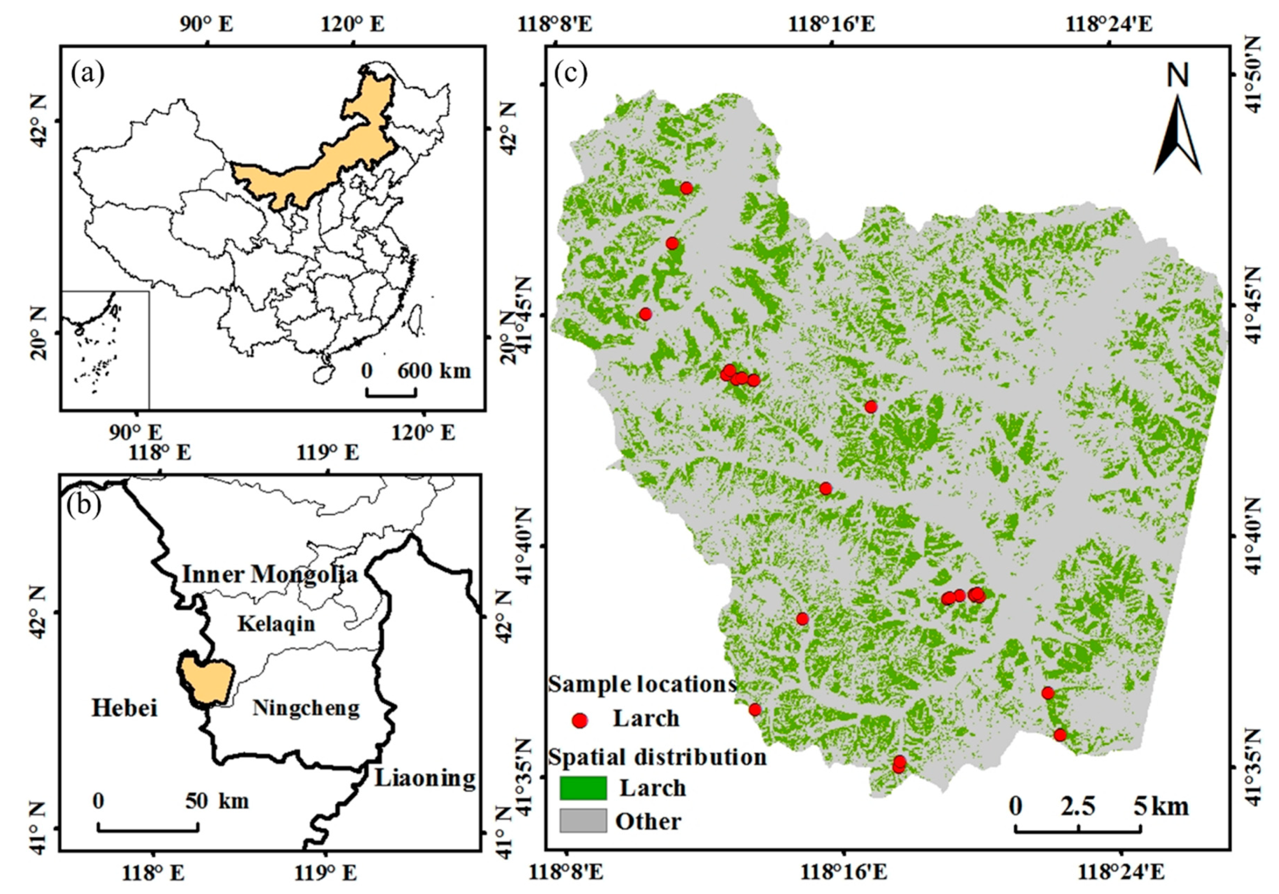
2.1. Study Area

The study area is the Wangyedian Experimental Forest Farm, located in the southwest of Harqin Banner, Chifeng city, Inner Mongolia Autonomous Region, and at the junction of three provinces—Inner Mongolia, Hebei, and Liaoning (see Figure 1). The study area has a total area of about 500 km2 with a distance of about 28 km north–south and 30 km east–west. By the end of 2016, forest cover accounted for about 93% of the total study area with a total stock volume of 1.52 million m3. This region has undulating topography with an elevation range of 500–1890 m. The climate belongs to temperate continental monsoon, having four distinct seasons: dry and windy in spring, rainy with high temperatures in summer, early frost in fall, and cold with little snow in winter. The average annual temperature is between 3.5 °C to 7 °C and the average annual precipitation is about 400 mm [35,36]. The dominant forest types include coniferous plantations (e.g., larch (Larix principis-rupprechtii and Larix olgensis), Scots pine (Pinus sylvestris), and Chinese pine (Pinus tabuliformis)) and secondary broadleaf forests such as Mongolian oak (Quercus mongolica), birch (Betula dahurica, Betula platyphylla), and aspen (Populus davidiana) [37]. On the basis of our previous research on forest classification, larch plantation in this farm has an area of 133.89 km2, accounting for 26.8% of the study area (see Figure 1c) [38].
Larch is a deciduous tree species in the genus Larix, of the family Pinaceae. With their cold-tolerant merit among coniferous tree species, larch is found in the plain of northernmost boreal zones and in the mountains of the temperate zones. A variety of Larix species including Larix gmelinii, Larix olgrnsis var. changpaiensis, Larix kaempferi, Larix principis-rupprechtii, and Larix sibirica grow naturally and are artificially cultivated, particularly in the northeast, north, and southwest China [39,40]. Larch plantation is one of the dominant forest types in the northeast [41] and is an important resource of timber production, providing a large amount of commercial timber products, as well as playing an important role in the forest ecosystem due to their high photosynthetic capacities and carbon fixation [42,43]. Therefore, the updating of larch forest AGB estimate in a timely manner is valuable for better understanding the carbon dynamics of larch plantations.

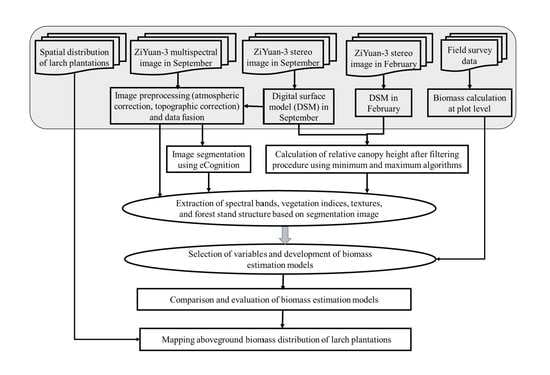
2.2. The Strategy of Forest Biomass Estimation using ZiYuan-3 Multispectral and Stereo Data

The framework of this research is illustrated in Figure 2, including (1) data preparation, covering collection of field inventory data for calculation of AGB at sample plot level, collection of multitemporal ZY-3 images and preprocessing, extraction of DSM from ZY-3 stereo images at different dates, collection of the extracted larch plantations from ZY-3 data [38], and image segmentation using eCognition; (2) extraction of potential variables such as vegetation indices and textural images from the fused multispectral data, and calculation of forest canopy features on the basis of the difference of bi-temporal DSM data; (3) selection of variables using stepwise regression and development of AGB estimation models based on different scenarios; and finally (4) evaluation of the modeling results and prediction of AGB distribution of larch plantations in the study area.

2.3. Data Preparation

The datasets used in this research are described in Table 1. Fieldwork was conducted in September/October 2017. Sample plots with a size of 25 by 25 m were allocated on the basis of the predefined rules—representative of the specific forest types, within the same forest site without crossing any different land cover types, away from the forest boundaries, and representative of different forest age groups. The coordinates for each plot were recorded. For each plot in the larch plantations, topographic factors (e.g., slope, aspect) and plantation age were recorded, and diameter at breast height (DBH) and tree height for individual trees were measured. A total of 24 plots were measured, and their spatial distribution is illustrated in Figure 1c.
In general, allometric equations are often used to calculate individual tree AGB using field measurements of DBH and tree height [25,44]. However, in reality, tree height measurement is often difficult, especially in mountainous regions. Therefore, the DBH-only models are often used for AGB estimation [44]. In this research, we conducted a comparative analysis of AGB estimates using the allometric equations with DBH-only models and using both DBH and tree height, finding high AGB differences for the similar DBH size within the same plot or among different plots. This was because the measure of tree height has high uncertainties from visual estimation by different persons. Therefore, this research selected a DBH-only equation (Equation (1)) to calculate the AGB of an individual tree [44,45].
l o g Y = 1.977 + 2.451 l o g D ,   R 2 =   0.971
where Y is AGB (unit: Mg) for a single tree, and D is the DBH–diameter at breast height (cm). The AGB of all trees within the same sample plot (25 by 25 m) were summed up as AGB amount at plot level, then converted to AGB at the hectare level (i.e., Mg/ha).
In previous research, Xie et al. [38] detailed the preprocessing of ZY-3 images (e.g., atmospheric and topographic correction), extraction of DSM from ZY-3 stereo images, fusion of multispectral and panchromatic data into a new data set using Gram–Schmidt fusion approach, as well as forest classification; thus, we will not repeat this here. Those data sources were directly used as inputs in this research. The image segmentation was conducted using eCognition software on the basis of the fused multispectral imagery with 2 m spatial resolution. The shape weight and compact weight were set as 0.2 and 0.5, and the scale of the segment was set as 250 after a substantial number of adjustments on the basis of the analysis of patch sizes of larch plantations. The segmentation image was further used to extract different variables from the fused ZY-3 multispectral data and DSM for AGB modeling.

2.4. Extraction of Potential Variables

2.4.1. Extraction of Spectral and Spatial Features

Vegetation indices can reduce the impacts of environmental conditions and have been proven valuable in improving AGB estimation, especially for the forest types with relatively simple stand structure [7,13]. The vegetation indices based on the available spectral bands in the ZY-3 multispectral imagery were summarized in Table 2.
In addition to spectral features, texture is another important variable in AGB estimation [5,7,8]. The gray-level co-occurrence matrix (GLCM) is a commonly used measure for extracting textural images [46]. Previous research on extracting textures required the determination of a suitable window size, specific spectral band, and texture measure, resulting in a large number of potential textural images [47]. However, not all these textural images are needed for AGB modeling. Therefore, it is critical to identify proper textural images that have a strong relationships with AGB but weak relationships between these textural images [7]. In fact, it is hard to identify an optimal window size and texture measure because of the different patch sizes of land covers. In order to avoid the selection of a window size, we extracted textures on the basis of the segmentation image, which was developed using eCognition based on the fused ZY-3 multispectral imagery. Eight texture measures—mean, standard deviation, homogeneity, contrast, dissimilarity, entropy, second moment, and correlation [46] were used to calculate textures on the basis of different spectral bands and segmentation image.

2.4.2. Extraction of Forest Canopy Features on the Basis of Bi-Temporal Digital Surface Model Data

In this research, we selected two seasonal ZY-3 stereo images (i.e., February and September) to extract DSM data (see details in [38]). For the February DSM image (leaf-off season), the minimum filtering approach using window sizes from 3 × 3 to 23 × 23 pixels were tested to produce DEM datasets, whereas for the September DSM image (leaf-on season), the maximum filtering approach using window sizes from 3 × 3 to 23 × 23 pixels were tested to produce DSM datasets. It was assumed that for deciduous forests such as larch plantations in this research, the minimum DSM in leaf-off season can be regarded as bare ground elevation, and the maximum DSM in leaf-on season can be regarded as surface elevation. Therefore, the relative canopy height (RCH) can be extracted using Equation (2):
RCH = DSMmax(September)−DSMmin(February).
Because of the strong relationship between AGB and canopy height, it is crucial to accurately extract the canopy height for the development of AGB estimation models. Therefore, the relationships between RCH from different window sizes (i.e., from 3 × 3 to 23 × 23 pixels) and AGB amount were examined to identify an optimal window size to extract the RCH image. Finally, on the basis of the selected RCH image for larch plantations, forest canopy features were calculated from this RCH image using the GLCM based on the segmentation image.

2.5. Selection of Variables and Development of Biomass Estimation Models

Although many approaches, such as machine learning algorithms, are used for AGB estimation [5,10], linear regression is still a common approach and has been proven to provide good prediction performance [10]. We used linear regression to establish AGB estimation models on the basis of two scenarios: (1) combination of spectral and spatial variables; and (2) combination of spectral, spatial, and forest canopy features, in order to understand whether the incorporation of forest canopy features into spectral and spatial data can reduce the data saturation problem in AGB estimation.
The stepwise regression analysis was used to identify the variables for AGB estimation modeling. Because the number of variables was greater than the number of sample plots, correlation analysis was first examined to explore the relationships between potential variables and AGB and between potentially explanatory variables. Only the variables having significant relationships with AGB but weak relationships with other explanatory variables were selected. The coefficient of determination (R2) and adjusted R2 were used to evaluate regression models. Meanwhile, the standardized Beta coefficients (Beta) were used to explain the relative importance of the selected variables in the regression model. A larger absolute Beta value indicates more importance of this variable in the model.

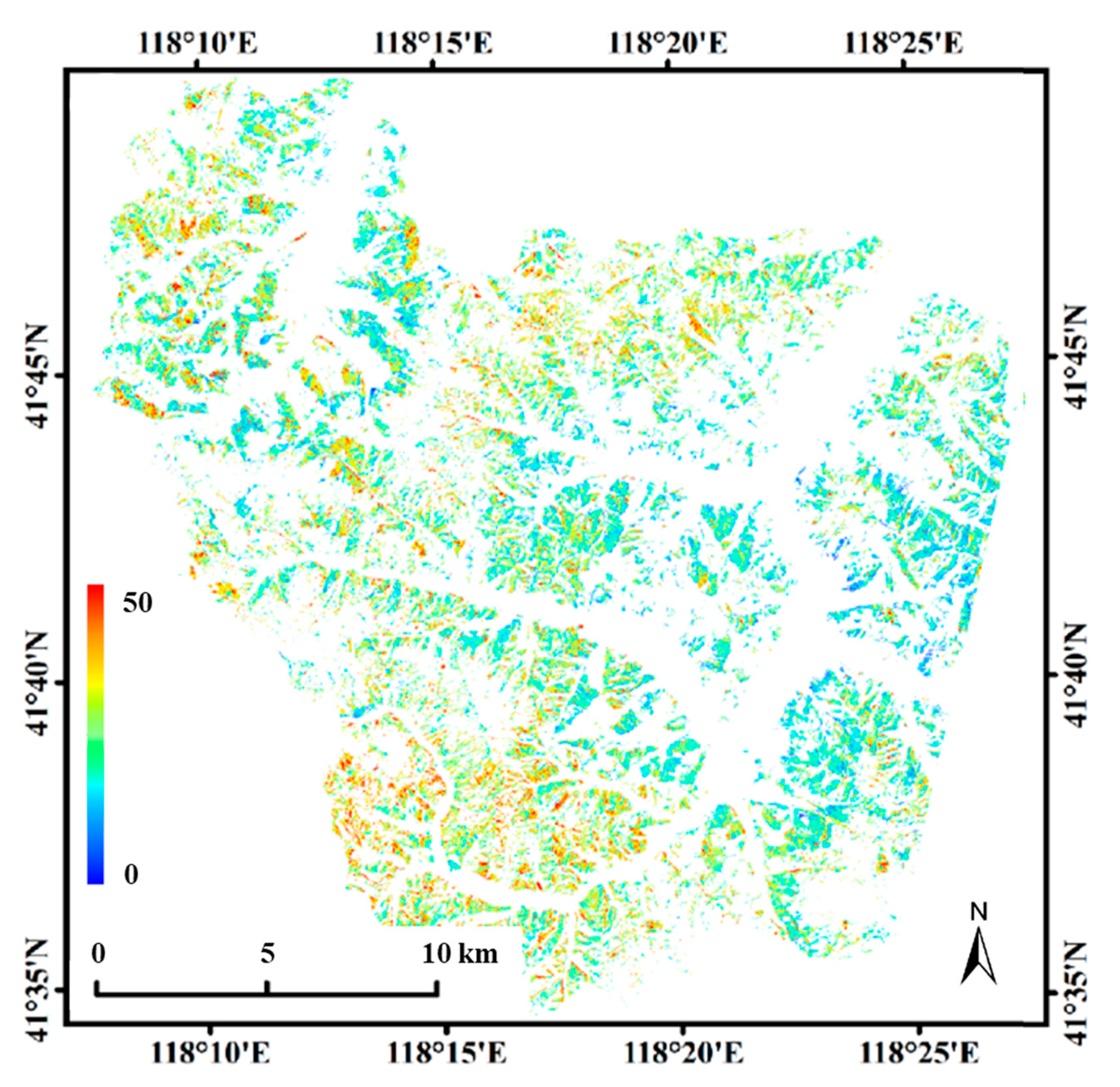
2.6. Evaluation of Modeling Results and Application of the Developed Model for Prediction of Biomass Distribution

The evaluation of modeling results is required for understanding the AGB estimation performance. In most case studies, the sample plots are randomly separated into two groups: modeling samples and validation samples [5,10]. However, collection of a sufficient number of samples for modeling and validation is often difficult because of the labor and cost, as well as accessibility. In order to solve this problem, an alternative is to divide the sample plots into k folds (here k is the number of sample plots) and use cross-validation for the model evaluation, that is, k-1 folds are used for model calibration and the remaining one fold is used for model validation, and this process is iterated for k times. In this research, we used the leave-one-out cross-validation for calculating correlation coefficient (r), root mean squared error (RMSE), relative RMSE (RMSEr), and mean absolute error (MAE) to assess the models’ prediction performance [16]. The higher r value and lower RMSE, RMSEr, and MAE values indicate better modeling performance. Meanwhile, the relationship between predicted AGB and reference data, as well as their residuals, were examined. The finally developed AGB estimation model was used to predict AGB spatial distribution of the entire study area.

3. Results

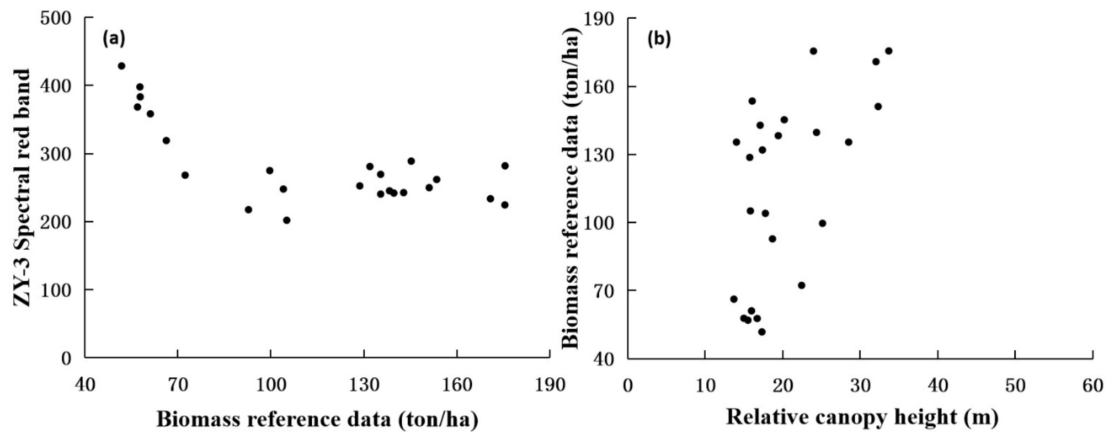
3.1. Analysis of the Role of Relative Canopy Height in Reducing Data Saturation Problem

The relationships between AGB and RCH images from different window sizes were examined, and it was found that the RCH image using the window size of 9 × 9 pixels provided the best result. Thus, this RCH image was used for extraction of forest stand features using GLCM. The examples in Figure 3 indicate that RCH has good linear relationships with AGB without the data saturation problem. However, different window sizes had various relationships between RCH and AGB, and the window size of 9 × 9 pixels provided the highest R2 value when compared with any other window sizes (Figure 3). The spatial distribution of RCH in Figure 4 indicates that most of pixels in this study area had RCH values between 10 and 30 m.
Previous research has shown the data saturation problem in optical sensor data and how the saturation values varied by forest types [7]. This research also showed the data saturation problem in ZY-3 multispectral data. The scatterplot between red spectral band and AGB (Figure 5a) shows that saturation value in ZY-3 data is about 110 Mg/ha for larch plantation in this study area. This implies that when AGB for a given site is greater than 110 Mg/ha, ZY-3 spectral bands cannot effectively predict AGB, resulting in large underestimation. On the other hand, the scatterplot consisting of AGB reference data and RCH (Figure 5b) indicates a linear trend; that is, when RCH increased, AGB increased also, implying that there was no data saturation problem when using RCH for AGB modeling.

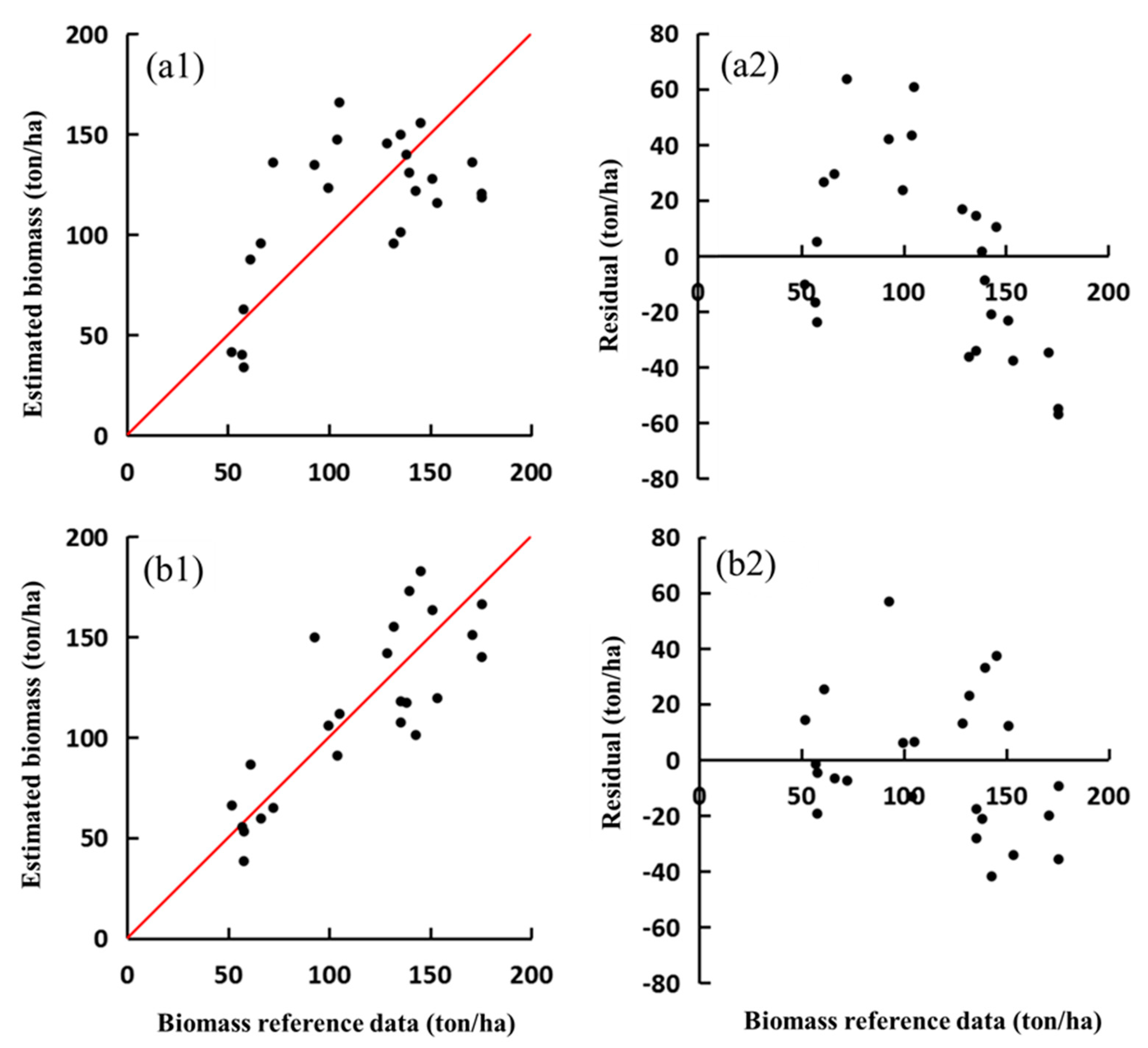
3.2. Analysis of Biomass Modeling Results

The selected variables for AGB modeling indicated that when the potential variables were based on spectral bands, vegetation indices, and textural images, only one variable—the red spectral band—was selected for AGB estimation using the linear regression approach. However, when multiple source data such as forest canopy features and spectral-derived variables were used, three variables—RCH, StdRCH, and red spectral band—were finally selected in the linear regression model (Table 3). The modeling R2 and adjusted R2 values in Table 3 indicated that the combination of canopy features and spectral band considerably improved the modeling performance when compared with the red spectral band alone. The F-test results indicated that the linear regression models were statistically significant, and Beta values showed that the spectral band still played an important role in AGB modeling, but also that the variables relating to forest stand structure (RCH and StdRCH) had significant roles in AGB modeling.
The evaluation of modeling results using r, RMSE, RMSEr, and MAE also indicated a considerable improvement through the incorporation of RCH features into spectral signature (Table 4). For example, because of the use of RCH features in AGB modeling, the correlation coefficients between AGB reference data and estimates increased from 0.616 to 0.825, implying an improvement in model prediction performance. The RMSE and MAE reduced from 33.89 (Mg/ha) and 30.68 Mg/ha) to 24.49 (Mg/ha) and 20.37 Mg/ha, respectively, and RMSEr decreased from 29.57% to 21.37%, implying that RCH indeed played an important role in reducing AGB estimation errors.
The scatterplots using the estimated AGB and corresponding reference data (Figure 6(a1 vs b1)) showed a better linear relationship using the RCH-based features (Figure 6b1) than using the spectral band alone (Figure 6a1). Although the residual figures (Figure 6(a2 vs b2)) looked similar, the absolute values were considerably different, especially for the samples with large residual values. For example, Figure 6a2 shows that two samples had residual values of over 60 Mg/ha, and another two samples had over 40 Mg/ha, whereas Figure 6b2 shows that only one sample had residual value of over 40 Mg/ha. A similar situation was that two samples had residual values near −60 Mg/ha, and four samples close to −40 Mg/ha in Figure 6a2; in contrast, only three samples were near −40 Mg/ha in Figure 6b2. This situation shows that use of RCH features indeed considerably improved AGB estimation performance.
A comparison of the AGB prediction results (see Figure 7) indicated that the AGB estimation model using RCH features provided a much greater number of pixels with AGB values of greater than 140 Mg/ha compared with using spectral red band alone, implying the important role of RCH features in reducing data saturation problem in the optical sensor data.

4. Discussion

4.1. The Role of Spectral and Spatial Features in Biomass Estimation

Previous studies have proven that incorporation of spectral and spatial features improved AGB estimation performance [7,8,10]. However, this research showed that the red band from ZY-3 data with 2 m spatial resolution, instead of vegetation indices or textures, was selected in AGB estimation models for larch plantations in North China. This conclusion is consistent with previous studies on secondary forests in the tropical forest ecosystem [12] and forest plantations such as pine and Chinese fir in subtropical forest ecosystems, which have relatively homogenous forest canopy structures [7]. Although spatial information is much richer in ZY-3 imagery with 2 m spatial resolution than in Landsat imagery with 30 m, the texture variables with improved spatial features were not included in the AGB estimation models. The possible reason may be that AGB is a composite attribute that is related to crown size, tree height, DBH, and tree density, but high spatial resolution features in the optical sensor data cannot effectively capture the attributes of forest stand structure. The lack of shortwave infrared (SWIR) band in ZY-3 image is another shortage for AGB estimation because previous research has shown that the variables, including SWIR bands, have stronger relationships with AGB than other spectral bands [7,12,13].

4.2. Potential Solution to Reduce the Data Saturation Problem in Optical Sensor Data

Previous research has shown that different forest types have various data saturation values. For example, utilizing Landsat Thematic Mapper (TM) imagery, pine forest and mixed forest have AGB saturation values of over 150 Mg/ha, and Chinese fir and broadleaf forests have relatively lower saturation values at 143 Mg/ha and 123 Mg/ha, respectively, in western Zhejiang Province, a subtropical region in China [7,8,10]. This research indicates that on the basis of ZY-3 multispectral image, larch plantation in North China has an AGB saturation value of about 110 Mg/ha. Data saturation in optical sensor data is a serious problem that results in AGB underestimation. In order to improve AGB estimation, one critical issue is to reduce the data saturation problem. Although stratification of forest types and topography can improve AGB estimation [7,10], they cannot solve the data saturation problem. Current optical sensor data can only provide the land surface information, that is, horizontal features, and cannot capture vertical information. Therefore, effectively employing the forest stand features such as canopy height is critical in reducing the data saturation problem, as shown in this research.

4.3. The Role of Forest Canopy Features in Improving Biomass Estimation

Since tree height or canopy height is strongly related to AGB without the data saturation problem, height-based variable has been regarded as the best data source for AGB estimation [5,48]. In reality, lidar data are mainly captured through airplanes or unmanned aerial vehicles (UAV), implying that this kind of data is not always available for a specific study area, considering the cost and labor. An alternative is to use satellite stereo images for extracting DSM [28,34,38]. However, one DSM image cannot directly extract canopy height data without use of DEM or DTM data. Previous studies used the combination of stereo and lidar data, in which stereo image was used to produce DSM, and lidar data were used to produce DTM [17,32,33,49,50]. Because no lidar data are available in this research, we used two DSM images from leaf-off and leaf-on seasons to produce canopy height data. However, a direct comparison of RCH and height measure was not conducted because of the following reasons: (1) the RCH image from the difference of leaf-on and leaf-off DSM images is not a real canopy or tree height; (2) our measured tree height data were mainly visually estimated by field surveyors, resulting in large uncertainties in height values and low reliability for canopy height calculation. Although we are not sure the accuracy of the extracted RCH result, this research indicated its effectiveness in obtaining the canopy height information for deciduous forests, a similar conclusion as previously indicated [21].
As more satellite stereo data are available, incorporation of stereo image and optical sensor data will provide new data sources for better AGB estimation. In recent years, UAV has become an important means of acquiring high spatial resolution images, including lidar, stereo, hyperspectral, and multispectral images in typical sites [21,51,52]. The UAV lidar or stereo data will be valuable for accurately mapping forest AGB distribution at the local scale [21]. Since ground survey is expensive and sometimes inaccessible for remote mountainous regions, UAV and satellite stereo data will play an important role in providing spatial distribution of AGB in the future. This research proved the potential of using stereo images in improving AGB estimation of larch plantations. This is especially valuable for deciduous forest AGB estimation.

4.4. Implication of Using Multiple Data Sources in Biomass Estimation

Previous studies have indicated the difficulty in using optical sensor data for forest AGB estimation [5,16]. In order to improve estimation performance, different approaches, such as stratification of forest types and topographic factors, and use of machine learning algorithms, are explored [7,8,9,10]. However, these approaches have limited improvement, and cannot solve the fundamental problems of overestimation and underestimation. Overestimation occurs when AGB is small, whereas overestimation occurs when AGB reaches a certain value such as 120 Mg/ha for most of forest types [7]. For a forest site with small AGB, its canopy is often not dense enough to cover the ground; thus, grass, shrubs, and bare soils under the canopy have considerable influence on the surface reflectance, resulting in high uncertainty in AGB estimation when only optical sensor data are used [5]. In contrast, for a forest site with very high AGB, data saturation becomes the major problem, resulting in AGB underestimation, as optical sensor data can only capture the canopy features without information of vertical features such as tree heights [7]. In order to improve AGB estimation, it is critical to incorporate different data sources, especially the canopy height relevant variables into AGB modeling [17,18,52]. This research shows that incorporation of surface feature (red spectral band), vertical feature (canopy height: RCH), and canopy structure (standard deviation of RCH) considerably improved AGB estimation, including the improvement of over- and under-estimation problems. This implies the importance of using different data sources in AGB modeling.
AGB is affected by many factors including soil conditions (e.g., soil structure, organic matter, soil fertility, soil moisture), topographic factors (e.g., elevation, aspect), and human-induced activities (different forms of management such as selective logging). Current AGB estimation models are mainly based on remotely sensed data without taking ancillary data into account [5]. More research should be explored to identify key variables from different data sources and develop suitable models that can effectively include different kinds of variables. However, different source data have various quality problems and spatial resolutions—there is a trade-off on how to use different data sources in forest AGB modeling. More research is needed to explore effective incorporation of remote sensing-derived products into the process-based ecosystem models for better understanding of the spatial distribution and dynamics of forest AGB.

5. Conclusions

This research explored the incorporation of ZY-3 multispectral and stereo imagery for AGB estimation of larch plantations in North China. The RCH was developed from the difference of bi-temporal DSM data that were extracted from leaf-on and leaf-off ZY-3 stereo images. A comparative analysis of AGB estimation results indicated that (1) ZY-3 spectral data alone cannot effectively predict AGB distribution of larch plantations, in particular, the data saturation problem resulted in serious AGB underestimation when forest AGB was greater than 150 Mg/ha; (2) the RCH based on bi-temporal DSM data can reduce the data saturation problem of spectral data. Incorporation of spectral and RCH variables considerably improved AGB estimation performance when compared with spectral data alone. RMSE and RMSEr were reduced from 33.89 Mg/ha and 29.57%, respectively, using the spectral data alone, to 24.49 Mg/ha and 21.37%, respectively, using the RCH-based combination. This research provides a feasible way to accurately predict AGB at high spatial resolution for deciduous forests using the combination of spectral and stereo images. As stereo images are available from different satellite sensor data, the approach used in this research will be valuable for regional AGB estimation for deciduous forests. Because AGB is related to tree species, DBH, tree height, age, and tree density, effective incorporation of different data sources (optical, lidar, radar, stereo) into the AGB modeling procedure will be an important research trend in near future. As airborne or space-borne lidar and satellite stereo data are easily available, combination of these data sets will be valuable in improving AGB estimation.

Author Contributions

Conceptualization, D.L. and E.C.; methodology, D.L., G.L., and E.C.; software, Z.X. and X.J.; validation, Z.X. and G.L.; formal analysis, Z.X., X.J., and G.L.; investigation, Z.X., X.J., G.L., and D.L.; resources, Z.X. and X.J.; data curation, X.J. and G.L.; writing—original draft, G.L. and D.L.; writing—review and editing, D.L., G.L., and E.C.; visualization, D.L.; supervision, D.L.; project administration, D.L. and E.C.; funding acquisition, D.L. and E.C.

Funding

This study was financially supported by the National Natural Science Foundation of China (grant #41571411) and by the National Key R&D Program of China project “Research of Key Technologies for Monitoring Forest Plantation Resources” (2017YFD0600900).

Acknowledgments

The authors would like to thank Lei Zhao, Longwei Li, Xiaozhi Yu, and Yahui Wang for their help in data collection. In particular, the authors would like to thank Yudong Jin from the Wangyedian Experimental Forest Farm, Chifeng, Inner Mongolia Autonomous Region, for his great support during field work.

Conflicts of Interest

The authors declare no conflicts of interest.

References

  1. Lu, D. The potential and challenge of remote sensing–based biomass estimation. Int. J. Remote Sens. 2006, 27, 1297–1328. [Google Scholar] [CrossRef]
  2. Nafiseh, G.; Reza, S.; Ali, M. A review on biomass estimation methods using synthetic aperture radar data. Int. J. Geomat. Geosci. 2011, 1, 776–788. [Google Scholar]
  3. Song, C. Optical remote sensing of forest leaf area index and biomass. Prog. Phys. Geog. 2012, 37, 98–113. [Google Scholar] [CrossRef]
  4. Kumar, L.; Sinha, P.; Taylor, S.; Alqurashi, A.F. Review of the use of remote sensing for biomass estimation to support renewable energy generation. J. Appl. Remote Sens. 2015, 9, 097696. [Google Scholar] [CrossRef]
  5. Lu, D.; Chen, Q.; Wang, G.; Liu, L.; Li, G.; Moran, E. A survey of remote sensing-based aboveground biomass estimation methods in forest ecosystems. Int. J. Digit Earth 2016, 9, 63–105. [Google Scholar] [CrossRef]
  6. White, J.; Coops, N.; Wulder, M.; Wulder, M.; Thomas, H.; Piotr, T. Remote sensing technologies for enhancing forest inventories: A review. Can. J. Remote Sens. 2016, 42, 619–641. [Google Scholar] [CrossRef]
  7. Zhao, P.; Lu, D.; Wang, G.; Wu, C.; Huang, Y.; Yu, S. Examining spectral reflectance saturation in Landsat imagery and corresponding solutions to improve forest aboveground biomass estimation. Remote Sens. 2016, 8, 469. [Google Scholar] [CrossRef]
  8. Zhao, P.; Lu, D.; Wang, G.; Liu, L.; Li, D.; Zhu, J.; Yu, S. Forest aboveground biomass estimation in Zhejiang Province using the integration of Landsat TM and ALOS PALSAR data. Int. J. Appl. Earth Obs. 2016, 53, 1–15. [Google Scholar] [CrossRef]
  9. Feng, Y.; Lu, D.; Chen, Q.; Keller, M.; Moran, E.; dos-Santos, M.; Bolfe, E.; Batistella, M. Examining effective use of data sources and modeling algorithms for improving biomass estimation in a moist tropical forest of the Brazilian Amazon. Int. J. Digit Earth 2017, 10, 996–1016. [Google Scholar] [CrossRef]
  10. Gao, Y.; Lu, D.; Li, G.; Wang, G.; Chen, Q.; Liu, L.; Li, D. Comparative analysis of modeling algorithms for forest aboveground biomass estimation in a subtropical region. Remote Sens. 2018, 10, 627. [Google Scholar] [CrossRef]
  11. Foody, G.; Boyd, D.; Cutler, M. Predictive relations of tropical forest biomass from Landsat TM data and their transferability between regions. Remote Sens. Environ. 2003, 85, 463–474. [Google Scholar] [CrossRef]
  12. Lu, D. Aboveground biomass estimation using Landsat TM data in the Brazilian Amazon. Int. J. Remote Sens. 2005, 26, 2509–2525. [Google Scholar] [CrossRef]
  13. Lu, D.; Mausel, P.; Brondízio, E.; Moran, E. Relationships between forest stand parameters and Landsat Thematic Mapper spectral responses in the Brazilian Amazon Basin. For. Ecol. Manag. 2004, 198, 149–167. [Google Scholar] [CrossRef]
  14. Lu, D.; Chen, Q.; Wang, G.; Moran, E.; Batistella, M.; Zhang, M.; Laurin, G.; Saah, D. Aboveground forest biomass estimation with Landsat and LiDAR data and uncertainty analysis of the estimates. J. For. Res-Jpn. 2012, 16. [Google Scholar] [CrossRef]
  15. Lu, D.; Batistella, M.; Moran, E. Satellite estimation of aboveground biomass and impacts of forest stand structure. Photogramm. Eng. Rem S. 2005, 71, 967–974. [Google Scholar] [CrossRef]
  16. Chen, Y.; Li, L.; Lu, D.; Li, D. Exploring bamboo forest aboveground biomass estimation using Sentinel-2 data. Remote Sens. 2019, 11, 7. [Google Scholar] [CrossRef]
  17. Mora, B.; Michael, A.; Joanne, C.; Geordie, H. Modeling stand height, volume, and biomass from very high spatial resolution satellite imagery and samples of airborne LiDAR. Remote Sens. 2013, 5, 2308–2326. [Google Scholar] [CrossRef]
  18. Maack, J.; Kattenborn, T.; Fassnacht, F.E.; Enßle, F.; Hernández, J.; Corvalán, P.; Koch, B. Modeling forest biomass using Very-High-Resolution data—Combining textural, spectral and photogrammetric predictors derived from spaceborne stereo images. Eur. J. Remote Sens. 2015, 48, 245–261. [Google Scholar] [CrossRef]
  19. Sousa, A.M.O.; Gonçalves, A.C.; Mesquita, P.; da Silva, J.R.M. Biomass estimation with high resolution satellite images: A case study of Quercus rotundifolia. ISPRS J. Photogramm. Remote Sens. 2015, 101, 69–79. [Google Scholar] [CrossRef] [Green Version]
  20. Macedo, F.; Adélia, M.; Ana, C.; José, R.; Marques, D.; Paulo, A.; Ricardo, A. Above-ground biomass estimation for Quercus rotundifolia using vegetation indices derived from high spatial resolution satellite images. Eur. J. Remote Sens. 2018, 51, 932–944. [Google Scholar] [CrossRef]
  21. Ni, W.; Zhang, Z.; Sun, G.; Liu, Q. Modeling the stereoscopic features of mountainous forest landscapes for the extraction of forest heights from stereo imagery. Remote Sens. 2019, 11, 1222. [Google Scholar] [CrossRef]
  22. Næsset, E.; Gobakken, T.; Bollandsås, O.; Gregoire, T.; Nelson, R.; Ståhl, G. Comparison of precision of biomass estimates in regional field sample surveys and airborne LiDAR-assisted surveys in Hedmark County, Norway. Remote Sens. Environ. 2013, 130, 108–120. [Google Scholar] [CrossRef] [Green Version]
  23. Mascaro, J.; Detto, M.; Asner, G.; Muller-Landau, H. Evaluating uncertainty in mapping forest carbon with airborne LiDAR. Remote Sens. Environ. 2011, 115, 3770–3774. [Google Scholar] [CrossRef]
  24. Lefsky, M.; Cohen, W.; Harding, D.; Parker, G.; Acker, S.; Gower, S. Lidar remote sensing of above-ground biomass in three biomes. Global Ecol. Biogeogr. 2002, 11, 393–399. [Google Scholar] [CrossRef] [Green Version]
  25. Chen, Q.; Vaglio, L.G.; Battles, J.; Saah, D. Integration of airborne lidar and vegetation types derived from aerial photography for mapping aboveground live biomass. Remote Sens. Environ. 2012, 121, 108–117. [Google Scholar] [CrossRef]
  26. Chen, Q.; Lu, D.; Keller, M.; Dos-Santos, M.; Bolfe, E.; Feng, Y.; Wang, C. Modeling and mapping agroforestry aboveground biomass in the Brazilian Amazon using airborne Lidar data. Remote Sens. 2016, 8, 21. [Google Scholar] [CrossRef]
  27. Chen, Q. Lidar remote sensing of vegetation biomass. In Remote Sensing of Natural Resources; Wang, G., Weng, Q., Eds.; CRC Press: Boca Raton, FL, USA, 2013; pp. 399–420. [Google Scholar]
  28. Shean, D.; Alexandrov, O.; Moratto, Z.; Smith, B.; Joughin, I.; Porter, C.; Morin, P. An automated, open-source pipeline for mass production of digital elevation models (DEMs) from very-high-resolution commercial stereo satellite imagery. ISPRS J. Photogramm. Remote Sens. 2016, 116, 101–117. [Google Scholar] [CrossRef] [Green Version]
  29. Goldbergs, G.; Maier, S.; Levick, S.; Andrew, E. Limitations of high resolution satellite stereo imagery for estimating canopy height in Australian tropical savannas. Int. J. Appl. Earth Obs. 2019, 75, 83–95. [Google Scholar] [CrossRef]
  30. Ni, W.; Dong, J.; Sun, G.; Zhang, J.; Pang, Y.; Tian, X.; Li, Z.; Chen, E. Synthesis of leaf-on and leaf-off unmanned aerial vehicle (UAV) stereo imagery for the inventory of aboveground biomass of deciduous forests. Remote Sens. 2019, 11, 889. [Google Scholar] [CrossRef]
  31. St-Onge, B.; Grandin, S. Estimating the height and basal area at individual tree and plot levels in Canadian Subarctic Lichen Woodlands using stereo WorldView-3 images. Remote Sens. 2019, 11, 248. [Google Scholar] [CrossRef]
  32. Persson, H.; Wallerman, J.; Olsson, H.; Fransson, J. Estimating forest biomass and height using optical stereo satellite data and a DTM from laser scanning data. Can. J. Remote Sens. 2013, 39, 251–262. [Google Scholar] [CrossRef]
  33. Vastaranta, M.; Markus, H.; Karjalainen, M.; Kankare, V.; Hyyppä, J.; Kaasalainen, S. TerraSAR-X stereo radargrammetry and airborne scanning LiDAR height metrics in imputation of forest aboveground biomass and stem volume. IEEE T Geosci. Remote 2014, 52, 1197. [Google Scholar] [CrossRef]
  34. Ni, W.; Sun, G.; Ranson, K.J.; Pang, Y.; Zhang, Z.; Yao, W. Extraction of ground surface elevation from ZY-3 winter stereo imagery over deciduous forested areas. Remote Sens. Environ. 2015, 159, 194–202. [Google Scholar] [CrossRef]
  35. Zhang, N.; Feng, Z.; Feng, Y.; Fan, J. Research on coniferous forest volume estimation model for Wangyedian experimental forest farm. J. Cent. South Univ. For. Technol. 2013, 33, 83–87. [Google Scholar]
  36. Feng, Z.; Xie, M.; Gao, Y. Evaluation on the woodland resource value in Wangyedian trial forest farm. For. Invent. Plan. 2014, 29, 60–65. [Google Scholar]
  37. Wu, C.; Ma, C. Struggle for sixty years, dream and flourishing industry—Record of development of Wangye Dian Experimental Forest Farm in Chifeng, the Inner Mongolia Autonomous Region. Land Green. 2015, 7, 16–19. [Google Scholar]
  38. Xie, Z.; Chen, Y.; Lu, D.; Li, G.; Chen, E. Classification of land cover, forest, and tree species classes with ZiYuan-3 multispectral and stereo data. Remote Sens. 2019, 11, 164. [Google Scholar] [CrossRef]
  39. Wang, X.Y.; Sun, Y.J.; Ma, W. Biomass and carbon storage distribution of different density in Larix olgensis plantation. J. Fujian Coll. For. 2011, 3, 221–226. [Google Scholar]
  40. Zhou, G.; Wang, Y.; Jiang, Y.L.; Yang, Z.Y. Estimating biomass and net primary production from forest inventory data: A case study of China’s Larix forests. For. Ecol. Manag. 2002, 169, 149–157. [Google Scholar] [CrossRef]
  41. Yang, K.; Zhu, J.; Zhang, M.; Yan, Q.; Sun, O. Soil microbial biomass carbon and nitrogen in forest ecosystems of Northeast China: A comparison between natural secondary forest and larch plantation. J. Plant Ecol-Uk 2010, 3, 175–182. [Google Scholar] [CrossRef]
  42. Gower, S.; Richards, J. Larches: Deciduous conifers in an evergreen world-in their harsh environments, these unique conifers support a net carbon gain similar to evergreens. Biosci. 1990, 40, 818–826. [Google Scholar] [CrossRef]
  43. Koike, T.; Yazaki, K.; Funada, R.; Maruyama, Y.; Mori, S.; Sasa, K. Forest health and vitality in northern Japan: A history of larch plantation. Res. Note Fac Forestry Univ. Joensuu. 2000, 92, 49–60. [Google Scholar]
  44. Wang, C. Biomass allometric equations for 10 co-occuring tree species in Chinese temperate forests. For. Ecol. Manag. 2006, 222, 9–16. [Google Scholar] [CrossRef]
  45. Ni, W.; Sun, G.; Guo, Z.; Zhang, Z.; He, Y.; Huang, W. Retrieval of forest biomass from ALOS PALSAR data using a lookup table method. IEEE J. Sel. Top. Appl. Earth Obs. Remote Sens. 2013, 6, 875–886. [Google Scholar] [CrossRef]
  46. Haralick, R.; Shanmugam, K.; Dinstein, I. Textural features for image classification. IEEE Trans. Syst. Man Cybern. Syst. 1973, 3, 610–620. [Google Scholar] [CrossRef]
  47. Lu, D.; Batistella, M. Exploring TM image texture and its relationships with biomass estimation in Rondônia, Brazilian Amazon. Acta Amazônica 2005, 35, 249–257. [Google Scholar] [CrossRef]
  48. Dong, P.; Chen, Q. Lidar Remote Sensing and Applications; CRC Press: Boca Raton, FL, USA, 2017; p. 220. [Google Scholar] [CrossRef]
  49. St-Onge, B.; Hu, Y.; Vega, C. Mapping the height and above-ground biomass of a mixed forest using lidar and stereo IKONOS images. Int. J. Remote Sens. 2008, 29, 1277–1294. [Google Scholar] [CrossRef]
  50. Torresan, C.; Berton, A.; Carotenuto, F.; Di Gennaro, S.; Gioli, B.; Matese, A.; Miglietta, F.; Vagnoli, C.; Zaldei, A.; Wallace, L. Forestry applications of UAVs in Europe: A review. Int. J. Remote Sens. 2017, 38, 2427–2447. [Google Scholar] [CrossRef]
  51. Ni, W.; Kenneth, J.; Zhang, Z.; Sun, G. Features of point clouds synthesized from multi-view ALOS/PRISM data and comparisons with LiDAR data in forested areas. Remote Sens. Environ. 2014, 149, 47–57. [Google Scholar] [CrossRef] [Green Version]
  52. Zhang, Z.; Ni, W.; Sun, G.; Huang, W.; Ranson, K.; Cook, B.; Guo, Z. Biomass retrieval from L-band polarimetric UAVSAR backscatter and PRISM stereo imagery. Remote Sens. Environ. 2017, 194, 331–346. [Google Scholar] [CrossRef]
Figure 1. The study area: (a,b) the location of the study area in North China, (c) larch spatial distribution and surveyed sample locations.
Remotesensing 11 02328 g001
Figure 2. Framework of aboveground biomass estimation for larch plantations using ZiYuan-3 multispectral and stereo images.
Remotesensing 11 02328 g002
Figure 3. A comparison of the relationships between aboveground biomass and relative canopy height on the basis of different window sizes (a1–a4: window sizes of 5 × 5, 7 × 7, 9 × 9, and 11 × 11 pixels, respectively).
Remotesensing 11 02328 g003
Figure 4. The extracted relative canopy height (m) image of larch plantations.
Remotesensing 11 02328 g004
Figure 5. A comparison of the relationships (a) between aboveground biomass and spectral red band and (b) between aboveground biomass and relative canopy height.
Remotesensing 11 02328 g005
Figure 6. The scatterplots between biomass reference data and modeling results (a1,b1) and residuals (a2,b2) (note: a—modeling based on spectral signature, b—modeling based on the combination of spectral and forest canopy features; 1—relationship between biomass reference data and modeling results, 2—residuals).
Remotesensing 11 02328 g006
Figure 7. A comparison of aboveground biomass spatial distribution using only spectral signature (a1) and using a combination of spectral and forest canopy features (a2), showing more pixels with high aboveground biomass values in (a2) than in (a1).
Remotesensing 11 02328 g007
Table 1. A summary of data sets used in research.
DatasetsDescription Date of Data Collection
Field survey dataA total of 24 sample plots were collected with an aboveground biomass (AGB) range of 51.83–175.59 Mg/ha, average AGB of 114.58 Mg/ha, and standard deviation of 41.36 Mg/ha.September/October 2017
ZiYuan-3 (ZY-3) dataZY-3 data covered (1) four multispectral bands (three visible bands and one near-infrared band) with 5.8 m and (2) stereo imagery—nadir-view image with 2.1 m and backward and forward views with 3.5 m spatial resolution. After image preprocessing, the Gram–Schmidt tool was used to integrate multi-spectral and panchromatic data to produce a new dataset with a spatial resolution of 2 m. This fused image was used to produce a segmentation image using eCognition software [38].Two seasonal images: one ZY-3 image was acquired on 9 February 2015 with a sun elevation angle of 31.44° and azimuth angle of 163.06°; another ZY-3 image was acquired on 20 September 2017 with a sun elevation angle of 44.22° and azimuth angle of 148.18°.
Larch classification imageThe larch classification result was developed from ZY-3 data using support vector machine (SVM)—user’s and producer’s accuracy of 79.7% and 94.8%.Details were provided by Xie et al. [38].
Digital surface model (DSM) dataThe DSM data were extracted from ZY-3 stereo images in February and September, independently. This research directly used the results for calculation of relative canopy height (RCH) after post-processing of the bi-temporal DSM data.Details were provided by Xie et al. [38].
Table 2. Vegetation indices used in the research.
Vegetation IndicesEquations
Differenced vegetation index (DVI)NIR − Red
Infrared percentage vegetation index (IPVI)NIR/(NIR + Red)
Normalized difference vegetation index (NDVI)(NIR − Red)/(NIR + Red)
Normalized difference greenness index (NDGI)(Green − Red)/(Green + Red)
Normalized difference water index (NDWI)(Green − NIR)/(Green + NIR)
Ratio vegetation index (RVI)NIR/Red
Re-normalized difference vegetation index (RDVI) ( NIR Red ) / NIR + Red
Visible-band difference vegetation index (VDVI) ( Green Red ) + ( Green Blue ) Green + Red + Green + Blue
Optimized soil adjusted vegetation index (OSAVI)(NIR − Red)/(NIR + Red + 0.16)
Ratio of near-infrared (NIR) band to blue bandNIR/Blue
Table 3. Biomass estimation modeling results.
DataRegression ModelsR2AdjR2F-testBeta
Spectral data263.855−0.555SBRed0.590.5734.73−0.769
Combination of spectral and stereo data−13.475−0.487SBRed + 2.594RCH + 5.147StdRCH0.780.7523.99−0.7080.3140.279
Note: SBRed: spectral red band; RCH: relative canopy height; StdRCH: standard deviation based on RCH image. R2: the coefficient of determination from the linear regression models; AdjR2: adjusted R2; Beta: standardized Beta coefficients.
Table 4. A summary of evaluation results.
DatarRMSE (Mg/ha)RMSEr (%)MAE (Mg/ha)
Spectral data0.61633.8929.5730.68
Combination of spectral and stereo data0.82524.4921.3720.37
r: correlation coefficient between AGB reference data and estimates; RMSE and RMSEr: root mean squared error (Mg/ha) and relative RMSE (%), respectively; MAE: mean absolute error.

