Article

An Attempt to Improve Snow Depth Retrieval Using Satellite Microwave Radiometry for Rough Antarctic Sea Ice

1
Integrated Climate Data Center (ICDC), Center for Earth System Research and Sustainability (CEN), University of Hamburg, 20146 Hamburg, Germany
2
Polar Research Center (PolRec), Istanbul Technical University (ITU), 34940 Istanbul, Turkey
*
Author to whom correspondence should be addressed.
Remote Sens. 2019, 11(19), 2323; https://doi.org/10.3390/rs11192323
Submission received: 29 August 2019 / Revised: 25 September 2019 / Accepted: 1 October 2019 / Published: 5 October 2019

Abstract

:
Snow depth on sea ice is a major constituent of the marine cryosphere. It is a key parameter for the derivation of sea-ice thickness from satellite altimetry. One way to retrieve the basin-scale snow depth on sea ice is by satellite microwave radiometry. There is evidence from measurements and inter-comparison studies that current retrievals likely under-estimate the snow depth over deformed, rough sea ice. We follow up on an earlier study, where satellite passive microwave data were combined with information on the sea-ice topography from the satellite laser altimeter on board the Ice, Cloud and land Elevation Satellite (ICESat) in a hybrid approach. Such topography information is spatiotemporally limited because of ICESat’s operation mode. In this paper, we aim to derive a proxy for this topography information from satellite microwave radiometry. For this purpose, we co-locate parameters describing the sea-ice deformation taken from visual ship-based observations and the surface elevation standard deviation derived from ICESat laser altimetry with the microwave brightness temperatures (TB) measured via the Advanced Microwave Scanning Radiometer aboard Earth Observation Satellite (AMSR-E) and aboard Global Change Observation Mission-Water 1 (GCOM-W1) (AMSR2). We find that the TB polarization ratio at 6.9 GHz and the TB gradient ratio between 10.7 GHz (horizontal polarization) and 6.9 GHz (vertical polarization), might be suited as such a proxy. Using this proxy, we modify the above-mentioned hybrid approach and compute the snow depths on sea ice from the AMSR-E and AMSR2 data. We compare our snow depths with those of the commonly used approach, the hybrid approach, with the ship-based observations for the years 2002 through 2015 and with the measurements made by drifting buoys for the period of 2014 through 2018. We find a convincing overall agreement with the hybrid approach and some improvement over the common approach. However, our approach is sensitive to the presence of thin ice—here, the retrieved snow depths are too large; and our approach performs sub-optimally over old ice—here, the retrieved snow depths are too small. More investigations and, in particular, more evaluations are required to optimize our approach so that the snow depths retrieved for the combined AMSR-E/AMSR2 period could serve as a data set for sea-ice thickness retrieval based on satellite altimetry.

Graphical Abstract

1. Introduction

Snow on sea ice is a major component of the marine cryosphere. It reduces the absorption of solar radiation, it reduces the atmosphere-ocean heat exchange, it insulates the sea ice against a cold or warm atmosphere [1], it modifies the aerodynamic properties of the sea ice [2,3], and it can contribute to the sea-ice volume when transformed into snow ice [4,5]. Additionally, snow plays a key role for the remote sensing of the sea-ice cover. Here, we focus on its role in the retrieval of the sea-ice thickness. Most currently used approaches for deriving the sea-ice thickness from satellite observations on a hemispheric scale use laser or radar altimeter observations in combination with Archimedes’ principle of buoyancy (e.g., [6,7,8,9,10,11,12]). With altimetry, the freeboard, i.e., the part of the sea ice above the sea surface, is obtained. With laser altimetry, one obtains the total (sea ice plus snow) freeboard (e.g., [13]). With radar altimetry, one obtains the sea-ice freeboard—provided the radar signal completely penetrates the overlying snow [6,9]. The conversion of the freeboard into the sea-ice thickness applying Archimedes’ principle requires the snow depth as an input parameter, among others (e.g., [10]). When using radar altimeter data, the snow depth is additionally required, to account for the signal delay in the snow when computing the sea-ice freeboard [8,14].
Hemispheric-scale snow-depth on sea-ice data products do exist (e.g., [15]). These are based on the brightness temperature observed by satellite passive microwave sensors such as the Special Sensor Microwave/Imager (SSM/I) or Advanced Microwave Scanning Radiometer (AMSR-E). The main algorithm behind these data sets uses the brightness-temperature gradient ratio at frequencies near 37 GHz and 19 GHz, both vertical polarizations, which has been regressed against a collection of ship-borne, in-situ and helicopter-borne snow depth measurements [16]. The algorithm has been developed for Antarctic sea ice [16,17], but it can also be applied to Arctic sea ice (here, to seasonal (first-year) sea ice only (e.g., [18])). The maximum snow depth to be retrieved is ~0.5 m.
A number of snow properties influence the accuracy of the retrieved snow depth. Among these are the grain size, snow density and snow wetness [16]. The influence of the snow wetness (connected to the snow temperature) and the snow grain size (connected to temporal snow temperature variations) can be reduced by applying a brightness temperature threshold and temporal averaging, e.g., over five days, respectively. Another important parameter influencing the retrieval is the surface roughness or degree of deformation. The surface roughness modifies the local incidence angle of the microwave radiation; it is ~53° for a horizontal surface for the employed satellite microwave radiometers. The snow depths on sea ice products are accurate for level sea ice (e.g., [18,19,20]). For deformed sea ice, however, the snow depths in the Antarctic are substantially under-estimated [19,21,22], confirming the results from the modeling [23] and air-borne campaigns in the Arctic [24]. This under-estimation of the snow depth results in a serious over-estimation of the sea-ice thickness when used in the above-mentioned sea-ice thickness retrieval algorithms (e.g., [25,26]).
Currently, several alternatives exist. These either aim to enhance the accuracy of the retrieved snow depth in general and/or to expand the retrieval to deeper snow and multiyear ice. Ozsoy-Cicek et al. [27] illustrated that measurements of the total freeboard can be used to obtain the snow depth on sea ice via a linear regression approach. Following this idea, Kern and Ozsoy-Cicek [28] used laser altimeter observations of the total freeboard of the Ice, Cloud and land Elevation Satellite ICESat’s Geophysical Laser Acquisition System (GLAS) to derive the snow depth of Antarctic sea ice. Xu et al. [29] developed a joint Soil Moisture and Ocean Salinity (SMOS) L-Band brightness temperature—CryoSat-2 approach to retrieve both the sea-ice thickness and snow depth at the same time in the Arctic. Guerreiro et al. [30] investigated the potential to combine two radar altimeters, CryoSat-2 and SARAL/AltiKa, to estimate the snow depth on sea ice in the Arctic. Rostosky et al. [31] modified the algorithm of Markus and Cavalieri [16] by including low-frequency information of the 10.7 GHz channels of the AMSR-E sensor to enhance the algorithm performance toward a potential application over multiyear ice and for deeper snow. Maass et al. [32,33] developed an algorithm based on SMOS brightness temperatures to estimate the snow depth over Arctic multiyear ice. All these approaches have one or two drawbacks: None of these specifically targets an improvement of the accuracy for deformed sea ice. None of these, except the one of Rostosky et al. [31], can be used to obtain hemispheric-scale, daily (or 5-daily) maps of the snow-depth distribution required for sea-ice thickness retrieval using, e.g., radar altimetry of Envisat RA-2 and CryoSat-2 [8]. Note however that the approach of Rostosky et al. [31] is developed for the Arctic, while the focus of the present paper is the Antarctic.
In the present paper, we expand the work of Markus et al. [22]. They illustrated that a combination of the approach of [16] with information about the sea-ice topography results in a substantial improvement of the snow depth retrieved for Antarctic sea ice. For this improvement, they combined AMSR-E brightness temperatures with the co-located total freeboard spatial standard deviation computed from along-track ICESat GLAS elevation measurements [22]; the improvement in accuracy was particularly substantial for deformed sea ice/deep snow. In our contribution, we attempt to replace the surface topography information given by the ICESat data, because of its poor spatiotemporal coverage, with a proxy for the surface topography information obtained from satellite microwave radiometry, i.e. AMSR-E and its successor AMSR2 aboard GCOM-W1.
Our paper is organized as follows. After this introduction, we describe the data used in Section 2. In Section 3, we check the quality of the input data and describe our approach. The results are shown in Section 4 and are discussed in Section 5. Section 6 concludes this paper.

2. Data

2.1. Ship-Based Observations

The observations carried out from aboard ships traversing sea ice provide valuable information about the sea-ice conditions. In the Antarctic, such observations have been carried out under the so-called ASPeCt (Antarctic Sea Ice Processes & Climate, http://aspect.antarctica.gov.au/) protocol [34,35,36] since the 1980s. ASPeCt observations are carried out manually from a voluntary observer at the ship’s bridge, who observes the sea ice around the ship within a radius of 1 km distance. Because the ship usually moves during an observation, the observation area has an elliptical shape; the semi-minor axis is 1 km, and the semi-major axis depends on the ships’ speed, the ice conditions, and the observers’ skills; an approximate average estimate of the observation footprint would be 2 km across-track times 5 km along-track. ASPeCt observations comprise the total sea-ice concentration and partial concentrations of the three thickest sea-ice types within sight. The additional parameters observed are the level sea-ice thickness, snow cover status and depth, ice type and floe size, ridge fraction and height, as well as a suite of meteorological parameters. For more information we refer to [35,36]. ASPeCt observations have been used in the past for various purposes (e.g., [21,28,34,37,38]).
In the present paper, we use the ASPeCt observations for two purposes. The first one is to investigate the relation between the brightness-temperature gradient ratios and polarization ratios and the observed surface topography, aka the height and distribution of ridges. The second one is to compare the snow depths computed from the AMSR-E and AMSR2 data with actual observations. We use an updated and extended version of the original ASPeCt data set (www.aspect.aq, ends in 2005) which extends from June 2002 through December 2015 ([39] last accessed 12 April 2019]. Figure 1 illustrates the spatiotemporal coverage of this extended ASPeCt data set.
For the quality check (Section 3.1), algorithm development (Section 3.2), and evaluation of the retrieved snow depth (Section 4.2) with the ASPeCt observations, we compute the mean values of the required parameters. These are the sea-ice thickness, snow depth, ridge height, and fraction of ridged ice. The mean values are computed using the observed fractions of the up-to-three ice types observed as weight. If Vi, i = 1, 2, 3 is the value of one of these parameters for the ice type i, e.g., the snow depth, Ci, i = 1, 2, 3 is the fraction of the ice type i, and C is the total sea-ice concentration, then the mean value is given by:
V = 1 C × ( C 1 × V 1 + C 2 × V 2 + C 3 × V 3 ) .
Equation (1) is modified accordingly if only one or two ice types are present. Note that we use the sea-ice thickness only as a threshold to exclude thin ice, as will be motivated later.
For the co-location with the satellite-based snow depths (see Section 4.2), we convert the latitude and longitude coordinates of both data sets into cartesian coordinates. That way, we search for the closest satellite grid-cell center by means of the minimum distance between an ASPeCt observation and the grid-cell center in kilometers. All comparisons using such co-located snow depth data are carried out using the daily, along-track mean values, i.e., we average over all co-located ship-observations and satellite product grid cells within one day, following the approach of Beitsch et al. [38]. By computing such along-track daily mean values, we reduce the noise inherent in the ASPeCt observations caused by the (mostly) different experiences and skills of the observers and by the varying sizes of the observation footprints.

2.2. Brightness Temperatures

For the algorithm development, we use AMSR-E/AMSR2 brightness-temperature swath data co-located with the ASPeCt observations (Section 2.1) and ICESat observations (Section 2.3), as well as ERA-Interim re-analysis near-surface meteorological parameters such as the 2 m-air temperature. The AMSR-E/AMSR2 data sources and the co-location methodology are described in Pedersen et al. [40]. The respective co-located data set is the result of a joint effort of the European Space Agency-Climate Change Initiative (ESA-CCI) sea-ice-ecv project and the EU-H2020-SPICES project and is also available via [40]; note that we use version 3 of this data set [last accessed 22 June 2018]; changes made between version 3 and the actual version 6 of this product do not relate to the data we use.
For the computation of the snow depth, we use the daily gridded AMSR-E brightness-temperature data set at a 25 km grid resolution, provided by NSIDC: AE_SI25.003 ([15], last accessed 26 April 2018), and the unified daily gridded AMSR2 brightness-temperature data set at a 25 km grid resolution: AU_SI25.001 ([41], last accessed 18 May 2019). These data sets are provided on a polar-stereographic grid with a tangential plane at 70° latitude. We do not use the snow depth data based on the approach of Markus and Cavalieri [16], henceforth named NSIDC, which are provided in the same data sets as mentioned above but at a 12.5 km grid resolution ([42,43], last accessed 18 May 2019). These NSIDC snow depths are filtered, i.e., the above-mentioned (in Section 1) 5-day running mean is applied [42,43]. Because we aim for an inter-comparison of our algorithm with unfiltered NSIDC algorithm snow depths, we compute the NSIDC snow depths on our own, as described in Section 3.

2.3. ICESat Surface Roughness

We use GLAS/ICESat L2 sea-ice altimetry data (GLA13) of release 33 altimetry binary data [44]. We downloaded the data for the ICESat measurement periods 2A to 2E from the U.S. National Snow and Ice Data Center (NSIDC: http://nsidc.org/data/gla13.html). This data was used to compute the average along-track surface elevation and its standard deviation σf for moving (by one laser shot) ground-track segments of 50 km length, as described in Kern and Spreen [45]. This computation is carried out separately for every ICESat measurement period between 2A (October/November 2003 or ON03) and 2E (March/April 2009 or MA09) (see Table 1). We refer to [44] and [45] for further information.
For the co-location with the AMSR-E brightness temperatures (see [40]), we only used values every 5 km to reduce the computational cost. We did not compute the freeboard and its standard deviation to minimize the influence of potential errors in the elevation-to-freeboard conversion due to, e.g., a lack of leads (see [45]). The main parameter of interest for the algorithm development (see Section 3) is the surface elevation standard deviation, which we show in Figure 2 for all ICESat measurement periods; note that ND08 is split into the October and November/December data.
For the algorithm development, we chose to average over five temporally consecutive ICESat surface elevation standard deviation values; the ICESat values are given as a time-series of the along-track measurements. Because five such consecutive values can originate from different ICESat overpasses, we compute this average only if the geographic coordinates of all five temporally consecutive ICESat values differ by between 0.2° and 0.3° in latitude and 0.05° and 0.3° in longitude.

2.4. AWI Snow Buoy Data

For the evaluation of our snow-depth product, we use, in addition to the ASPeCt snow depth observations (Section 2.1), observations from the Alfred-Wegener Institute (AWI) snow buoys deployed in the Southern Ocean during the years 2013 until now. These buoys provide four coincident individual snow height measurements representing an area of ~10 m2 around the buoy carried out by a downward looking sonar mounted at a known fixed altitude above the ice-snow interface [46]. The measured snow heights have an accuracy of one centimeter and are stored hourly together with the position and the air temperature. The data are post-processed, and the outliers removed and made available via http://www.meereisportal.de [47,48].
For the inter-comparison (Section 4.2), we average over the up-to-four snow-depth measurements, i.e., use one value per position. Observations with fewer than three individual snow-depth buoy measurements are discarded. We co-locate the buoy and satellite data, as described in Section 2.1, for the ASPeCt data. We inter-compare the data using the daily mean values of both the buoy and satellite data, following the approach of Beitsch et al. [38].

3. Methodologies

3.1. Quality Check of the Input Data and Confirmation of Recent Findings

Here, we illustrate whether the data inputs into the development of our approach in Section 3.2 are related to each other as expected. First, we focus on the ASPeCt observations. We limit the investigation to total sea-ice concentrations > 90% and to sea-ice thickness > 0.3 m; a motivation for these thresholds is given in Section 3.2 in the context of Equation (3). We find, as expected, that the snow depths on sea ice increase with the sea-ice thickness (Figure 3a), that the sea-ice thickness is positively related to the fraction of ridged ice (Figure 3b), and that the snow depth on sea ice is also positively related to the fraction of ridged ice (Figure 3c). We refer in this context also to a recent paper where high-resolution observations are used to also illustrate the relationships between the sea-ice thickness and snow depth on the one hand and the degree of deformation on the other hand [49].
We compute the NSIDC AMSR-E snow depths using the brightness temperatures of the product AE_SI25.003 (Section 2.2), co-locate these with our ASPeCt data set, compute the difference of AMSR-E minus the ASPeCt snow depth, and display this difference as a function of the ridged ice fraction in the form of histograms (not shown). We find that for ridged ice fractions > 25%, the AMSR-E snow depths under-estimate the ASPeCt snow depths by 20 cm or more in ~30% of the cases. Conversely, for ridged ice fractions < 15%, the AMSR-E snow depths under-estimate the ASPeCt snow depths in only < 10% of the cases. The snow depth under-estimation by 40 cm or more occurs in ~10% of all cases with a high ridged ice fraction.
How do the AMSR-E NSIDC snow depth data distribute when co-located with other roughness information? Can we confirm our findings based on the ASPeCt observations? In order to answer this question, we co-locate the AMSR-E NSIDC snow depth data (see [22], Equation (1)) with the ICESat surface elevation standard deviation (Elevation STDDEV) and display the distribution of the AMSR-E snow depths, separately for the fall, winter and spring periods, for different ranges of the Elevation STDDEV: <0.05 m, 0.05 m to 0.1 m, …, >0.2 m (Figure 4). We find a pronounced mode in the snow depth distribution at depth values between 5 and 10 cm for values of the Elevation STDDEV < 0.15 m. For sea ice with a higher variability in the surface topography, 0.15 m to 0.2 m, and >0.2 m (orange and red graphs), we find modal snow depths of ~20 cm in fall and winter (see Figure 4a,b, orange and red arrows). In contrast, in spring (Figure 4c), we find these modes to be located at snow depths < 10 cm, like the modal snow depths of the other ranges of the elevation STDDEV. This is not a direct confirmation of the ASPeCt results. However, we take this finding as another confirmation of the results of Worby et al. [19] and Kern and Ozsoy-Cicek [28], who showed that the NSIDC AMSR-E snow depths tend to decrease from winter to spring, under-estimating the snow depth in particular during this season. It remains to be noted, however, that the thickest snow is associated with the two largest Elevation STDDEV classes.

3.2. Algorithm Development

Markus et al. [22] already suggested to combine the main parameter used for the AMSR-E snow depth retrieval: the brightness-temperature gradient ratio at 37 and 19 GHz (vertical polarization GR3719VV) corrected for the influence of open water (GRice) with the standard deviation of the total (sea ice + snow) freeboard σf derived from ICESat measurements. They proposed the following equation to compute an improved snow depth, which substantially reduces the negative bias over rough sea ice:
S = 5.45 638.67 × G R i c e + 1.21 × σ f .
In Figure 5, we illustrate, by means of a color-coded scatterplot, the distribution of the snow depth retrieved with the NSIDC algorithm (Figure 5a) and the Markus et al. [22] algorithm (Figure 5b) as a function of the GRice (y-axis) and ICESat elevation STDDEV (x-axis) for the spring ICESat measurement periods. The NSIDC AMSR-E snow depths distribute parallel to the x-axis across the GR3719VV–ICESat roughness (elevation STDDEV) space (Figure 5a); there is no variation of the retrieved snow depth with the elevation STDDEV. In addition, most snow depths are <0.5 m. In contrast, as expected, the Markus et al. [22] snow depths vary with both the GR3719VV and elevation STDDEV (Figure 5b). In addition, we find a considerable fraction of snow depths > 0.5 m. This is an encouraging result and agrees with the findings of, e.g., [50].
Markus et al. [22] and our study (for Figure 5b) combined the AMSR-E data with ICESat data. However, ICESat data was measured discontinuously (see Table 1). Therefore, until the launch of its successor, ICESat-2, in September 2018, the approach of Markus et al. [22] could only be applied to obtain an improved daily snow depth on sea ice for the Antarctic for the ICESat measurement periods (Table 1). This is suboptimal for sea-ice thickness retrieval from satellite altimetry.
Henceforth, we describe our approach to find a substitute for the surface topography proxy σf among the AMSR-E brightness temperatures. In a first step, we investigate which brightness-temperature gradient (GR) or polarization (PR) ratio shows a reasonable relationship with the observed surface topography. For this purpose, we derive the daily average ridged ice fraction and standard deviation from the ASPeCt observations of the ridge height during one day and compare these with the co-located daily average GR and PR values derived from the AMSR-E and AMSR2 brightness temperatures TB. We excluded cases with a <90% sea-ice concentration and sea-ice thickness < 0.3 m, and applied a 2m-air temperature threshold of −10 °C. By excluding cases with a <90% sea-ice concentration, we minimize the impact of open water on GR and PR. By excluding cases with a sea-ice thickness < 0.3 m, we attempt to minimize the influence of the emission of water underneath thin ice on GR and PR, recalling that penetration depths into sea ice increase with a decreasing frequency. Finally, by excluding cases warmer than −10 °C, we mitigate the influence that liquid water within the snow may have on the GR and PR values.
The GR values are computed as:
G R f 1 f 2 p 1 p 2 = ( T B f 1 p 1 T B f 2 p 2 ) T B f 1 p 1 + T B f 2 p 2 ,
with frequency f1 = {89.0 GHz, 36.5 GHz, 18.7 GHz, or 10.7 GHz}, frequency f2 = {36.5 GHz, 18.7 GHz, 10.7 GHz, or 6.9 GHz}, polarization at frequency f1: p1 = {V or H}, and polarization at frequency f2: p2 = {V or H}. Note that we use 89, 37, 19, 10, and 6 to denote these frequencies henceforth. The GR is computed for every combination of f1 with a smaller frequency f2, i.e., for example, GR3719, GR3710, and GR3706, and for every polarization combination, i.e. VV, VH, HV, and HH.
The PR values are computed as:
P R f = ( T B f p 1 T B f p 2 ) T B f p 1 + T B f p 2 ,
with frequency f = {89.0 GHz, 36.5 GHz, 18.7 GHz, 10.7 GHz, or 6.9 GHz} and polarizations p1 = V and p2 = H. The PR is computed once for every frequency. Note that despite setting a sea-ice concentration threshold of 90%, we follow Markus and Cavalieri [16] and derive the so-called “ice” version of all the GR and PR values by correcting them for a potential influence of open water. The tie points of open water required for this correction are taken from Tonboe and Pedersen [51] (their Table 2.4).
We focus on these ratios to mitigate the impact of (near-) surface temperature variations on the measured brightness temperature. We do not aim to replace GR3719VV in Equation (2) by another, potentially better suited GR or PR value (e.g., [31]) but aim to find a proxy for the surface topography. Observations [24] and modeling studies [23,52] confirm earlier findings (e.g., [53]) and suggest that, especially at lower frequencies, i.e., 10 GHz and 6 GHz, the brightness temperatures are sensitive to the surface topography. Furthermore, the other frequencies, i.e., 19 GHz through 89 GHz [52,53,54], are sensitive to surface topography variations. However, these higher frequencies are more sensitive to the snow depth and to other snow properties, such as the density and grain size, than the lower frequencies are. Moreover, the penetration depth of microwave radiation into snow is smaller for the higher frequencies than for the lower ones. Therefore, although AMSR-E frequencies exhibit a certain sensitivity to the surface topography of the snow and/or ice-snow interface, the sensitivity of the lower frequencies dominates over the other sensitivities because of the longer wavelength and deeper penetration of the microwave signal. We remind the reader that our aim here is to find a proxy for the variation of the surface topography. Hence, we wish to exclude other effects as much as possible; we therefore focus on GRs and PRs at the low frequencies.
We find high correlations between the ASPeCt ridged ice fraction, and PR06, PR10 and the gradient ratios GR1006HV and GR1006VH: 0.92, 0.84, −0.83, and 0.90, respectively (Figure 6a–d), which coincide with reasonably steep slopes of a linear regression. These values are valid for winter and decrease toward spring, when the correlations and slopes decrease to 0.41, 0.20, −0.30, and 0.66, respectively (Figure 6e–h). GR1006VH offers the highest overall correlation with the ridged ice fraction, and PR06 offers the second highest. Note that, together, winter and spring account for 88.6% of all values.
We find even higher correlations between the ASPeCt ridge height standard deviation and PR06, PR10, GR1006HV, and GR1006VH: 0.94, 0.94, −0.91, and 0.85, respectively (Figure 6i–l). We observe a reduction toward spring, which is less pronounced than for the ridged ice fraction; the correlation values are 0.66, 0.66, −0.72, and 0.82, respectively. Again, GR1006VH offers the highest overall correlation. The correlations and slopes obtained for GR1006VV and GR1006HH (not shown) are considerably smaller than those obtained for the cross-polarized GRs.
We also find a reasonable linear relationship between the PR and GR values with the two ASPeCt surface roughness parameters for fall (not shown here); the correlation coefficients range from |0.35| to |0.63| for the ridged ice fraction and |0.26| to |0.61| for the ridge height standard deviation. However, the number of data pairs is too small for us to follow up with this further.
The next step is to investigate the relationship of GR and/or PR with the co-located ICESat surface elevation standard deviation σf. We again carry out this investigation by means of two-dimensional histograms (comparable to Figure 6). Based on the results of the comparison with the ASPeCt data, we focus on the seasons of fall through spring for the low frequencies and available ICESat periods only.
Figure 7 illustrates the main results of our investigation regarding the relationship between the AMSR-E PR and GR values at the low frequencies and σf. We find the best (linear) relationships for fall and winter (left two columns in Figure 7) with the steeper slopes obtained for fall; a steeper slope means a larger sensitivity. For fall, we find the highest correlation for PR06 and GR1006HV: 0.73 and 0.72, respectively. For winter, we find the highest correlations for PR06 and PR10: 0.55 and 0.53, respectively; note that these are considerably smaller than those in fall. For spring, the correlations drop to almost zero, as do the slopes, meaning that the PRs and GRs that are used are not sensitive to σf. This is a discouraging result, especially in light of the fact that, unlike for the comparison with the ASPeCt observations where winter and spring accounted for ~90% of all the data, for the comparison with the ICESat data ~50% of the data pairs are from spring, ~15% from fall and ~30% from winter. We note that these results are insensitive to both the choice of the sea-ice concentration threshold (which can be seen as a proof that the correction of the GR and PR values for the open water influence is working well) and to the air temperature. All the above-described results are obtained from cold cases, e.g., air-temperatures < −10 °C; using higher temperature thresholds only increases the noise in the two-dimensional histograms in Figure 7 but not the general agreement between the two data sets.
Despite this obvious limitation, we perform the next step and replace σf in Equation (2) with the linear equation relating σf to a GR or PR (see the equations in black font in Figure 7). For PR06fall (Figure 7a), Equation (2) thus modifies into:
S = 5.45 638.67 × G R i c e + 1.21 × 100 × ( 6.846 × P R 06 i c e 0.213 ) .
The factor 100 converts from meters to centimeters. Figure 7 illustrates that the observed σf values barely fall below 0.03. The application of the linear regression, however, could result in a smaller or even negative computed σf. Therefore, if the computed σf falls below 0.03, we set it to 0.02.
We identify one issue with Equation (5). For a small computed σf, Equation (5) under-estimates the snow depths that would be obtained with the standard NSIDC algorithm (e.g., [22], Equation (1)):
S = 2.9 782.0 × G R i c e
for the same GRice as inserted into Equation (5). More specifically, for a typical range of GRice values between −0.01 and −0.06 and a computed σf of 0.02, one would under-estimate the snow depth by between ~5 cm and ~15 cm with Equation (5), when compared to Equation (6). Larger computed σf values of 0.05 or 0.08 would still result in a negative bias in the snow depth for the lower, i.e., more negative, GRice values. We decide to avoid this by combining Equations (5) and (6) as follows:
S = S E q u a t i o n ( 6 )   if   S E q u a t i o n ( 6 ) S E q u a t i o n ( 5 )   , otherwise   S = S E q u a t i o n ( 5 ) .
In Figure 8, we illustrate the effect of combining both equations over using just Equation (5). We use the co-located ASPeCt–AMSR-E/AMSR2 brightness temperature data set (Section 2.1) and compute the snow depth with the standard NSIDC algorithm, Equation (6), with an enhanced version of this algorithm, the so-called UB-SICCI [55,56] and with our algorithm, henceforth referred to as ITU algorithm. For the latter, we apply Equation (5) using PR06fall, PR06winter, a linear combination of both: PR06mixed, as well as the respective coefficients for GR1006HV, and we apply Equation (7) for the same set of PR and GR values. We compare the daily mean along-ship track values in Figure 8 and Table 3. Note that here and for all other retrieval results shown hereafter, the negative snow depths are set to 0 cm.
The histograms of the NSIDC and UB-SICCI snow depths (Figure 8a) agree well with the one of the ASPeCt snow depths. UB-SICCI exhibits slightly thicker snow depths than NSIDC. The histograms of the ITU snow depth agree less with the ASPeCt snow depths (Figure 8b–d). We find a considerably smaller count of snow depths between 10 cm and 20 cm. We find a considerably larger count of snow depths > 40 cm than observed (ASPeCt) and computed otherwise (NSIDC and UB-SICCI); there are actually no snow depths > 40 cm in NSIDC and UB-SICCI (Figure 8a). We find that the combination of NSIDC and ITU algorithms results in less variation of the counts among the three thinnest snow-depth bins 0–10 cm, 10–20 cm and 20–30 cm. The distributions most resembling the one of the ASPeCt snow depths in these three bins are PRfall2 and GRfall2 (Figure 8e). As expected, there is almost no change between Figure 8b–d and Figure 8e–g for snow depths > 30 cm.
Two issues need to be taken into account when interpreting Figure 8 and Table 3. First: the ASPeCt snow depths are supposed to be reported for level sea ice. Second: the ASPeCt observations are carried out while the ship navigates in ice-covered waters. The ship most often follows easy-to-navigate waters, i.e., open or freshly refrozen leads and/or level ice of the thinnest thickness category. Therefore, the ASPeCt snow depths are expected to be biased as being low compared to the actual snow depth (e.g., [19]). Having stated this, the differences between the snow depths obtained with the ITU algorithms and the ASPeCt observations shown in Figure 8 and Table 3 should be seen in a different light. While the agreement between the NSIDC/UB-SICCI snow depths and ASPeCt snow depths seems very good, this is based on a snow-depth distribution where deep snow is missing. Moreover, there is evidence that the NSIDC snow depths under-estimate the snow depth over deformed sea ice by a factor of two to three (e.g. [19]); a considerable fraction of the deep snow is missing. Our results, obtained with the ITU algorithm, provide a substantial fraction of snow deeper than that contained in the distributions shown in Figure 8a. We hypothesize that with our new algorithm we are able to uncover at least part of the deeper snow missing in the ASPeCt observations and in the snow-depth retrievals based on the NSIDC and UB-SICCI algorithms.

4. Results

4.1. Snow Depths from Co-Located Data Sets

First, we compute the snow depth for the co-located AMSR-E–ICESat data set with the aim to quantify the differences between ITU and the other snow-depth retrievals. We employ the same algorithms already used in Figure 8 and Table 3. In addition, we employ the Markus et al. [22] hybrid algorithm (henceforth Markus2011; see Equation (2) in the present paper), combining the AMSR-E brightness temperatures with the ICESat surface elevation standard deviation. For the ITU algorithm, we apply PR06, PR10, GR1006HV, and GR1006VH for fall, winter, all year, and the linear fall-winter combination “mixed” (see above).
In Figure 9, we show a subset of the obtained snow depth maps. The snow depths are only displayed at locations with valid ICESat surface elevation standard deviations, for sea-ice concentrations >90% and 2 m-air temperatures <−10 °C. The data for “Winter” are based on considerably fewer measurements (only ICESat measurement periods extending into June for the years 2004–2006) than the data for “Spring” (ICESat measurement periods overlapping with the months of September to November of the years 2003–2008; see Table 1).
In winter, the snow depth distributions are quite similar across the five algorithms shown. We find comparably high snow depths for the western Weddell Sea (red circle), and for parts of the Amundsen Sea and Ross Sea (red ellipse). Most other regions are dominated by comparably thin snow, i.e., the eastern Weddell Sea or southern Ross Sea. For the western Weddell Sea, we find the thickest snow and the largest spatial gradients. For this region in particular, it is evident that the maximum NSIDC snow depths (~50 cm) are smaller than those of Markus2011 and ITU (~80 cm). However, the locations where specific maximum snow depths appear often differ between Markus2011 and ITU (see Figure 8b–e, black arrows). For the western Weddell Sea (red circle), ITU PR06mixed reveals the smallest snow depths among the ITU implementations. Note that there are only a few valid ICESat data with sea-ice concentrations >90% off East Antarctica.
In spring, the differences between NSIDC (Figure 8f) and all other algorithms (Figure 8g–j) are larger than during winter. This applies to the entire sea-ice cover but mostly to the regions outlined by the red frames. Here, the NSIDC snow depths are often considerably smaller than the other snow depths. For example, for the western Weddell Sea (red circle), the maximum NSIDC snow depths are ~40 cm, while the Markus2011 and ITU snow depths peak at ~80cm and ~70 cm, respectively. The same is valid for the Amundsen Sea/Ross Sea region (red ellipse). While for the western Weddell Sea, the spatial distribution of the snow depth is quite similar between Markus2011 and ITU, we find considerable differences for the Amundsen Sea/Ross Sea region. Thick snow is mostly located south of 70°S in the map showing Markus2011 (Figure 8g). All three ITU snow-depth maps (Figure 8h–j) exhibit a patchier distribution of thick snow, which is not limited to the area south of 70°S (black arrows in Figure 8g–j).
For the eastern Weddell Sea, we find a fringe of elevated snow depths along the coast when using Markus2011 (Figure 8g) but not when using the NSIDC (Figure 8f) or the ITU algorithm (Figure 8h–j). Finally, in the sea-ice cover off East Antarctica (red rectangle), the Markus2011 snow depths are considerably larger than the NSIDC snow depths: the latter are ~10 cm, while the former peak at ~40 cm. ITU also provides elevated—compared to NSIDC—snow depths, but the high snow depths are more scattered along the coast than the Markus2011 snow depths are.
In Table 4, we present the results of the ITU algorithm implementations that provide the overall best agreement with Markus2011; the results for the other GRs and PRs are not shown. We highlight the results of the comparison with Markus2011 because our aim is to develop a similar snow-depth algorithm, with the surface topography proxy based on the ICESat data replaced by a surface topography proxy based on microwave radiometry; we are hence interested in as good an agreement to the Markus2011 snow depths as possible. Table 4 illustrates that ITU PR06 generally has the best performance, followed by ITU GR1006HV. The differences between the ITU and NSIDC snow depths are negative for all seasons, ranging between −4 cm and −10 cm. The differences between the ITU and Markus2011 snow depths are smaller: −2 cm to 2 cm, often near zero, e.g., PR06fall2: −0.1 cm for both fall and winter, and PR06mixed: 0.2 cm for spring. Generally, we find a smaller standard deviation of mean snow-depth differences between NSIDC and ITU than between Markus2011 and ITU. The correlations between the Markus2011 and ITU snow depths are largest for fall (~0.8) and smallest for spring (~0.6). We note that the NSIDC and Markus2011 snow depths are correlated similarly high for fall (0.92) and winter (0.90) but not for spring (0.75), which is when the Markus2011 snow depth exceeds the NSIDC snow depth by ~9 cm. Similar but slightly lower/higher values are found using an air-temperature threshold of −2 °C (not shown here). The correlations are a bit smaller overall. In spring, ITU GR1006HVfall provides better (=closer to Markus2011) results than ITU PR06fall. In spring, ITU PR10fall (not shown) also performs better than PR06mixed but worse than PR06fall and GR1006HVfall. However, we decided to avoid potential inconsistencies in snow-depth retrieval caused by combining different ITU implementations and do not mix these in different seasons.
In Table 5, we show the change in the mean snow depth between fall and winter and between winter and spring. Kern and Ozsoy-Cicek [28] found that the NSIDC snow depths tend to decrease from winter to spring, which was not confirmed in independent data. They hypothesized that this decrease could be caused partly by the under-estimation of the snow depth over deformed sea ice by the NSIDC algorithm. Following this hypothesis, we are inclined to choose an ITU implementation that has no or at least a smaller winter-to-spring decrease in snow depth than the NSIDC algorithm does. We find that Markus2011 is optimal, with a snow-depth change close to zero (Table 5). For the ITU implementations, PR06mixed is closest to the performance of Markus2011, followed by PR06fall and PR06mixed2. The GR1006HV implementations result in a winter-to-spring snow-depth decrease as large as the NSIDC algorithm. PR06fall2 is not performing optimally here but is still better than NSIDC (Table 5).
Based on the findings illustrated in Figure 8 and Figure 9 and Table 3, Table 4 and Table 5, we select PR06fall2 and GR1006HVfall2 (Equation (7)), as well as PR06mixed (i.e., Equation (5)), for further usage. We apply the equations (with the respective modification according to the selected implementation) to the daily gridded AMSR-E and AMSR2 brightness temperatures. We compute the snow depth using the ITU algorithm, the NSIDC algorithm and its enhanced version, UB-SICCI, for June 2002 through October 2011 and for July 2012 through December 2018.
It turns out that the ITU algorithm provides unrealistically high snow depths along the marginal ice zone and in polynya areas (see Section 5 for discussion). Therefore, we flag snow depths at sea-ice concentrations <90% as not usable. Note that the algorithm is not tailored to lower sea-ice concentrations but is developed based on high-concentration cases. In the following two subsections, we show the results of our comparison between these snow depth products and the independent snow-depth observations.

4.2. AMSR-E/AMSR2 Snow Depth Compared to Ship-Based Snow-Depth Observations

We compare the gridded snow depth product with the ASPeCt snow-depth observations performing the co-location, as described in Section 2.1. We perform this comparison separately for AMSR-E and AMSR2 and separately for the entire year, for winter (April to October) and summer (November to March). The results are given in Figure 10 and Figure 11 and in Table 6.
At first glance, none of the scatterplots shown in Figure 10 provides a convincing agreement between the AMSR-E and ASPeCt snow depth data. NSIDC and UB-SICCI (see Table 6) under-estimate the ASPeCt snow depths (Figure 10a–c). The mean difference is ~6 cm (~3 cm using UB-SICCI) with standard deviations of the difference between 10 cm and 13 cm. The linear correlation is below 0.4. The slope is 0.33 at maximum, suggesting a threefold steeper increase of ASPeCt than the satellite snow depths. We note in this context that the ASPeCt observations often under-estimate the true snow depth, as mentioned in the text associated with Figure 8.
ITU, in contrast, over-estimates the ASPeCt snow depths by ~5 cm (GR1006HVfall2, Figure 10j–l), 6 to 8 cm (PR06fall2, Figure 10d–f), or even 12 to 15 cm (PR06mixed, Figure 10g–i). The standard deviations of the difference are mostly larger, while the linear correlations are as low as those obtained using NSIDC and UB-SICCI. Larger slopes (0.4 to 0.6) suggest a better agreement between the satellite and ASPeCt snow depths, with less under-estimation than that obtained using NSIDC and UB-SICCI. However, the larger intercepts suggest that the ITU algorithm possibly over-estimates the small snow depths, independent of the implementation used. This is also evident in the scatterplots of Figure 10: the ITU snow depths spread between 0 and 60 cm over the ASPeCt snow-depth range of 0 to 20 cm. The main improvement between NSIDC and ITU is evident in the region denoted by the black ellipses. Here, most satellite snow-depth data move from being considerably below the identity line (Figure 10a) to being around the identity line (Figure 10d,g,j); this is most evident when using the two PR06 implementations. The mean satellite snow depths computed from the binned ASPeCt snow depths (red triangles) underline this reduction in the difference satellite-minus-ASPeCt snow depth particularly well. Using these averaged data, the squared correlations are 0.7 and 0.65 using NSIDC and UB-SICCI, increasing to 0.80, 0.82, and 0.83 using the ITU implementations PR06fall2, GR1006HVfall2, and PR06mixed, respectively. Comparing the scatterplots for summer and winter (Figure 10, middle and left columns) reveals that the majority of the above-mentioned improvements occur during summer.
For AMSR2 (Figure 11), we find almost no agreement between the satellite and ASPeCt snow depths. While we find mean differences close to 2 cm, the spread of the satellite snow depths for a given ASPeCt snow-depth range is huge (see Figure 11). In the data region where we find the best improvement for AMSR-E (Figure 10, black ellipses), we find only a slight improvement for AMSR2 (Figure 11, black ellipses)—mostly for ITU PR06. However, the shifts of the satellite snow depths toward the identity line are much smaller here compared to in Figure 10. We refer to Section 5 for a discussion of this discrepancy between the AMSR-E and AMSR2 results.

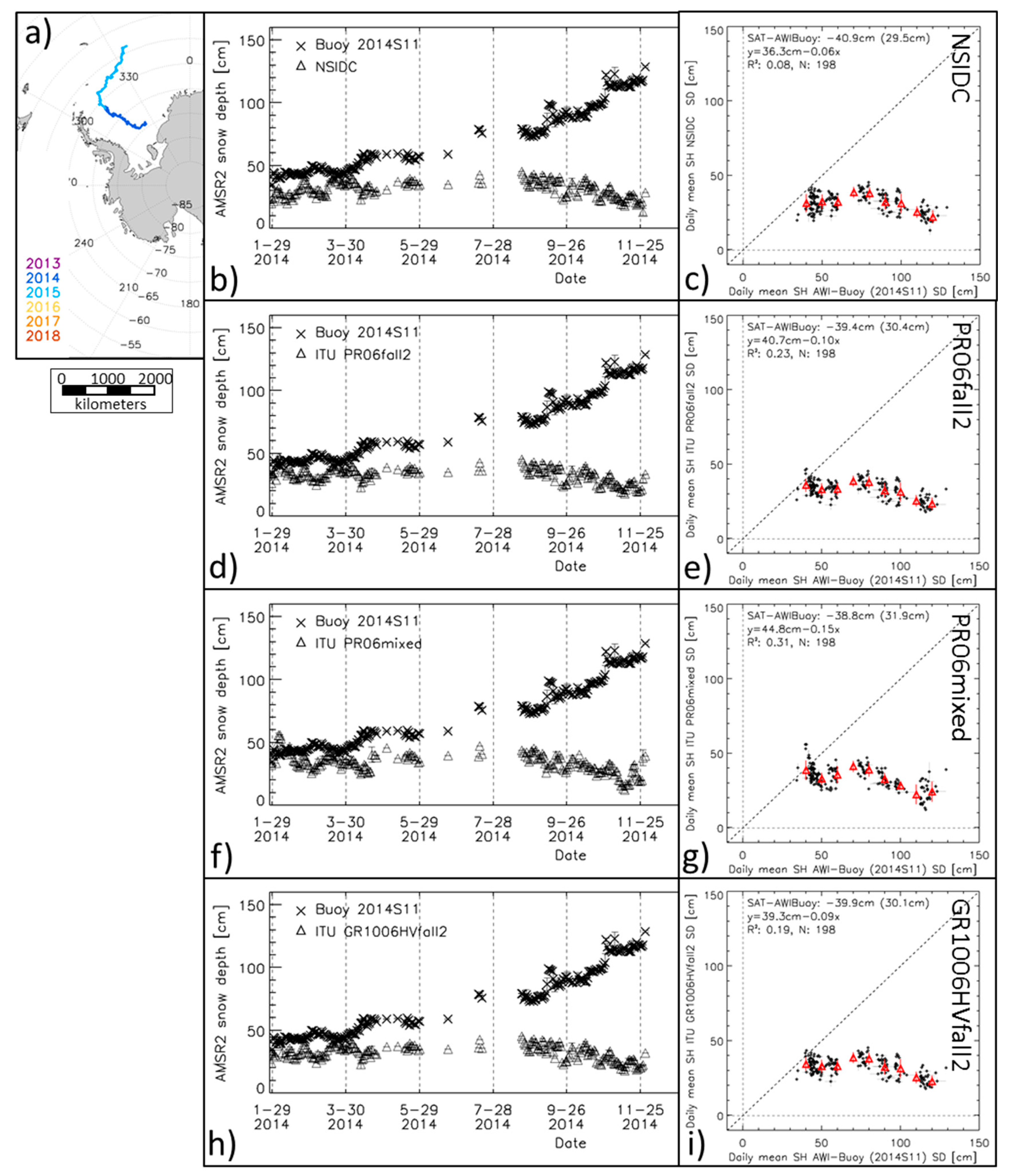
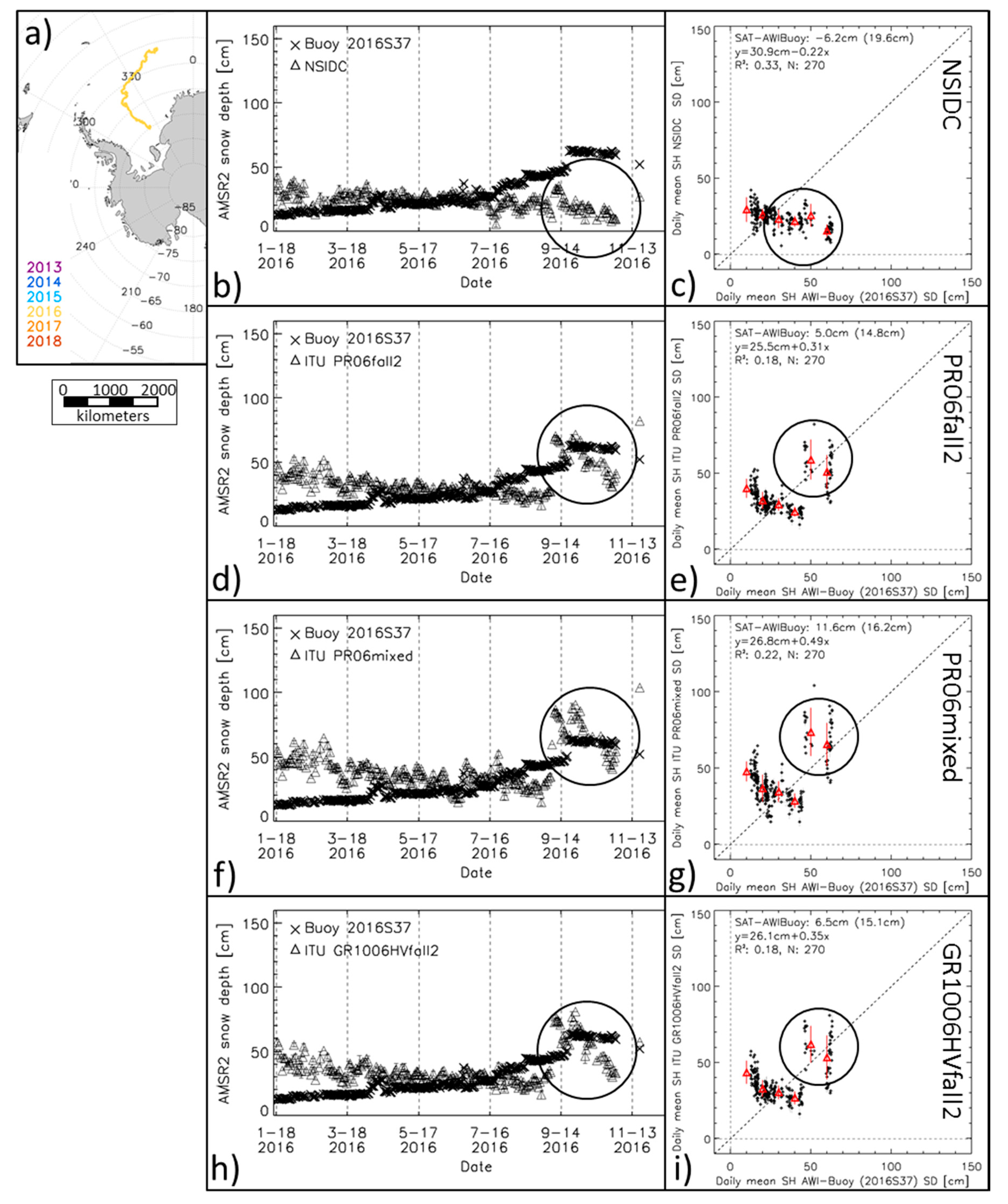
4.3. AMSR2 Snow Depth Compared to Buoy Snow-Depth Observations

We compare the gridded AMSR2 snow depths with the observations of the snow depth from 12 AWI snow depth buoys (Section 2.4). The co-location of the data is done the same way as for the ASPeCt observations, and the comparison is carried out using the daily mean values. The data are valid if the sea-ice concentration is > 90%, if the processing flag for the satellite snow depth retrieval denotes nominal retrieval, and if the air-temperature measured at the buoy is below −2 °C.
Buoy 2014S11 (Figure 12a) crossed the western Weddell Sea toward the north in 2014 before turning northeastward in 2015. Our valid data stop at the end of November 2014. The snow depth observed by the buoy was initially around 40 cm and stayed within 40 to 50 cm until the end of March. The snow depths increased gradually during April to ~60 cm. After a data gap from June through August, the snow depth was ~70 cm in the beginning of September. From then onward, the observed snow depth increased to ~110 cm at the end of November 2014.
None of the algorithms show the increase in snow depth observed by the buoy. All of the algorithms provide a relatively constant snow depth of ~35 cm for almost the entire period that was shown, even exhibiting a decrease in the snow depth starting in September to ~20 cm at the end of November. The overall mean differences between the snow depth data sets are therefore quite large. The correlations are low.
The tracks of buoy 2016S31 (Figure 13a) and 2016S37 (Figure 14a) are similar to those of buoy 2014S11 (Figure 12a), except that buoy 2016S31 circulated back toward the west. The snow depth development is similar for these two buoys.
At buoy 2016S31 (Figure 13), all algorithms reveal a larger snow depth than that observed by the buoy until about mid-July. The NSIDC snow depths (Figure 13b) are actually first quite close to the observations, before increasing to ~30 cm in mid-March and gradually decreasing to ~20 cm until mid-July. ITU provides a snow-depth maximum between ~50 cm (Figure 13h) and ~70 cm (Figure 13f) in mid-February before the snow depths decrease toward values between 20 cm and 30 cm until mid-July. Subsequently, the observations indicate a snow depth increase. The NSIDC snow depths first stay constant, then increase to ~50 cm for a short period of time, before subsequently decreasing to < 20 cm (Figure 13b, black circle). The ITU snow depths are also constant until the end of September and then increase to 50 cm or even more (Figure 13d,f,h, black circles), all exceeding the buoy observations. ITU PR06mixed shows the largest (and relatively constant) snow depth, while the ITU GR1006HVfall2 snow depths peak at ~60 cm, but then decrease to ~40 cm until mid-November. The black circles in the scatterplots (Figure 13, right column) illustrate well the shift in the snow-depth values from below the identity line (NSIDC) to above it (ITU).
We find a similar evolution of the AMSR2 snow depths at buoy 2016S37. The main differences to buoy 2016S31 are: (i) The NSIDC snow depths basically decrease for the entire period shown (Figure 14b); (ii) The agreement between the AMSR2 and buoy snow depth is better during the winter months of April through July; (iii) The ITU snow depths vary considerably more after the increase in mid-September (Figure 14d,f,h, black circles); and (iv) In particular, ITU PR06mixed is more variable throughout the entire period. Similar to Figure 13, the scatterplots (Figure 14, right column, black circles) illustrate the shift of data points from below the identity line for NSIDC (Figure 14c) to around it for all ITU implementations.

5. Discussion

Markus et al. [22] developed a hybrid approach to compute snow depth on Antarctic sea ice using AMSR-E brightness temperatures and, as a proxy for the surface topography, the ICESat surface elevation standard deviation (see Equation (2)). Our results suggest that this proxy could be replaced by brightness-temperature ratios computed from AMSR-E or AMSR2 measurements. The polarization ratio (PR) of the 6.9 GHz channel (PR06) or at the 10.7 GHz channel (PR10) could be used. Alternatively, the gradient ratio (GR) of these two channels at cross-polarization, i.e., 10.7 GHz (horizontal polarization (H)) and 6.9 GHz (vertical polarization (V)) or vice versa (GR1006HV, GR1006VH), could be used. We base this suggestion on (i) a comparison between the co-located visual ship-based observations of the parameters describing the surface topography (fraction of ridged ice and right height standard deviation) and the AMSR-E/AMSR2 brightness temperature ratios (Figure 6) and ii) a comparison between the latter and the co-located ICESat surface elevation standard deviations (Figure 7). Note that these comparisons are carried out for sea-ice covers with a >90% sea-ice concentration and are based on open-water influence corrected brightness temperature ratios (see [16]). We show how we modified the approach of [22], compute the snow depths for the period 2002 through 2018 (Figure 8 and Figure 9) and compare the results with independent snow depth observations (Figure 10, Figure 11, Figure 12, Figure 13 and Figure 14).

5.1. Differences in the Observations Themselves

There are fundamental differences between the observations. The surface topography proxy taken from ICESat depends on the number and height of the ridges and snow dunes and the levelling effect of the snow between the ridges; it is independent of processes within the snow or at the ice-snow interface. The surface topography information derived from the ship-based observations is also independent of the processes just mentioned; more importantly, it is only a measure of the surface topography caused by the ridges. In contrast, the brightness temperatures and ratios derived from these are more influenced by the topography of the ice-snow interface than by the actual surface topography. The change in the dielectric constant across the ice-snow interface is much larger than across the air-snow interface. At the frequencies used for the ITU algorithm to replace the surface topography proxy based on the ICESat data, the snow is more or less transparent as long as it is dry and cold and the volume scattering within the snow is small. Therefore, relationships such as those suggested from Figure 6 and, more importantly, Figure 7, are reliable as long as the ice-snow interface topography is a fair representation of the surface topography.
However, the weather conditions in the Antarctic are very variable. Surface winds are very variable, precipitation can be substantial and air temperatures can exceed the freezing point even during winter. It can be expected that by spring a large fraction of the sea-ice cover has experienced multiple advance and retreat cycles, melt and re-freeze cycles, several events of snow accumulation and redistribution, and also, potentially, several events of flooding and re-freezing (e.g., [4,57]). Therefore, not only does the surface topography spectrum change from fall to spring, but the relevant properties of the snow (number of ice layers, grain size, basal snow layer salinity, wetness) and the ice-snow interface (ice type, salinity, small-scale surface roughness, surface wetness) change as well. This variability in the relevant snow and ice-snow interface properties explains, in our opinion, (1) the scatter observed across the regression lines in Figure 7, and (2) the breakdown of the relationship between the ICESat surface elevation standard deviation and selected brightness temperatures ratios from fall to spring (see Table 2). Wherever such snow and ice-snow interface properties influence the relevant PR and GR values, the ITU algorithm snow depths might be biased. This can be either because these properties change PR/GR values so that smooth sea ice looks like rough sea ice, i.e., sea ice with a strongly varying ice-snow interface topography, or because the properties change the PR/GR values so that rough sea ice looks like smooth sea ice.
The penetration depth into sea ice at these low frequencies is substantial. For thin sea ice, a considerable fraction of the measured brightness temperature might actually emanate from the water underneath and be additionally influenced by the large vertical salinity gradient typical for thin ice. The PR is a function of the ice thickness for thin sea ice already at 18 and 37 GHz (e.g., [58]) and even more so at lower frequencies. The thinner the sea ice is, the larger the PR is. Because of this, thin ice might in particular look like rough sea ice (see Figure 7a,d) with consequences for ITU algorithm snow-depth retrieval. In our results, we find, for example, unrealistically large snow depths in the Ross Ice Shelf polynya as well as along the marginal ice zone, both being areas of elevated fractions of thin ice.

5.2. Differences in the Scales

There are fundamental differences between the scales of the input data. One individual ship-based observation represents an approximately two kilometer-wide by five kilometer-long area. For the daily along-track averages used, we average over up to 24 such observations (one observation per hour during a polar day). The ICESat surface elevation standard deviations are computed over segments of 50 km length along the track using all the valid individual single-shot surface elevation measurements within this segment. These individual values represent a footprint area of 70 m in diameter spaced ~170 m along the track, i.e., one surface topography value represents a transect of 50 km length. For the co-location with the AMSR-E data, these segments are shifted by 5 km along the track. Finally, the AMSR-E/AMSR2 brightness temperatures at the two low-frequency channels integrate over an elliptic area of 43 km × 75 km (6.9 GHz) and 29 km x 51 km (10.7 GHz).
The co-location with the ICESat data is carried out using individual AMSR-E footprints from individual satellite overpasses. The co-location with the ship-based observations uses daily gridded AMSR-E/AMSR2 brightness temperatures at a 25 km grid resolution. The consequence of this is that the co-located data shown in Figure 7 are not only based on a shorter time-period than those shown in Figure 6 but that these are also more instantaneous; Figure 7 involves much less averaging of the AMSR-E data than Figure 6 does. This fact again adds to the scatter observed in Figure 7.

5.3. Discussion of the Inter-Comparison Results

Overall, the tested and finally selected ITU implementations provide a good agreement with the Markus2011 snow depths (Table 4), prompting us to select the ITU implementation with the PR06, fall coefficients (see Figure 7) as the main implementation. We could show that, compared to the NSIDC algorithm, the ITU algorithm provides snow depths in good agreement with Markus2011. However, if we take a closer look, we find evidence of the issues discussed, especially in Section 5.1. For instance, the patchiness of the ITU snow depths compared to the Markus2011 snow depths observed in the Amundsen Sea/Bellingshausen Sea (Figure 9, red ellipses) is most likely the result of the above-mentioned changes in the relevant snow and ice-snow interface properties, simulating and/or obscuring the effect of rough ice on the measured brightness temperatures.
We note in this context that Markus et al. [22] developed the Markus2011 algorithm from the data of a limited region in the East Antarctic sea-ice cover and also evaluated their approach by a limited set of local snow depth in situ observations collected during the ARISE expedition in September/October 2003 [59]. This region is known for a large amount of deformed, often rafted sea ice (e.g., [60,61]) and exhibits different surface elevation properties than, e.g., the Weddell Sea or the Ross Sea (e.g., [27]). Therefore, we cannot expect that the Markus2011 and the ITU algorithm, which is developed so that it agrees with Markus2011 as much as possible, results in an improvement in snow depth on sea ice retrieval from satellite microwave radiometry for the entire Antarctic. The ICESat surface topography proxy used in the Markus2011 algorithm [22] is only sporadically available for up to three about 35-day long periods during the years 2003 through 2009 (see Table 1). Therefore, the Markus2011 algorithm can only be applied to these periods, as we did in this paper (see e.g., Figure 9). Since September 2018, ICESat-2 provides continuous measurements of the surface elevation, so that since then the method of [22] could be applied.
Our inter-comparisons with independent snow depth observations (Section 4.2 and Section 4.3) provide a mixed picture. When compared to the ship-based observations of 2002–2011, i.e., the AMSR-E period (Figure 10, Table 5), we find some improvements at thicker snow depths and a general shift from overly small to overly high snow depths for ITU compared to NSIDC or UB-SICCI. For the ship-based snow depth observations between 0 and 20 cm, we find a substantially higher scatter for ITU than NSIDC; we find this unrealistic and attribute it to the effect of other snow and ice properties than the ice-snow interface or surface topography and the presence of thin ice (Section 5.1). When compared to the ship-based observations of 2012–2015, i.e., the AMSR2 period (Figure 11), we find almost no improvement between NSIDC/UB-SICCI and ITU. We hypothesize that this could be caused by the fact that most of the data used here are from the Weddell Sea (compare Figure 1a), a region with different sea-ice properties than in East Antarctica, where [22] developed their approach.
This hypothesis is underlined by our comparison with the AWI snow buoy data shown in Figure 12, Figure 13 and Figure 14. The snow-depth time series, as well as the scatterplots derived for buoy 2014S11 (Figure 12), reveal a poor agreement between the buoy and satellite observations. The buoy snow depths are under-estimated by all satellite products by 10–20 cm during the beginning of the time series and by close to 100 cm at its end. In contrast, for buoy 2016S31 and buoy 2016S37, we find some improvement in the agreement between the buoy and satellite snow depth for ITU toward the end of the shown time series. Note, however, that the NSIDC snow depths tend to fit the buoy observations better than ITU during a substantial fraction of the time series. Of particular note is the good agreement between the NSIDC and buoy snow depths at the beginning of the time series of 2016S31 when all the ITU snow depths over-estimate the buoy snow depth by about 50 cm. It could be that this buoy—and also buoy 2016S37—were placed in an area of relatively thin ice and therefore elevated PR06 values, with the already-mentioned consequences for the ITU snow depth. Actually, the thin snow depths observed here suggest that this is first-year ice, while the thick snow present at the beginning for buoy 2014S11 suggests that this is old ice. The presence of old ice would actually also explain why, for buoy 2014S11, none of the ITU algorithms lead to an improvement. Old ice has different properties than first-year ice, which in our case could simulate low-frequency PR and GR values representative of smooth sea ice (compare Figure 7).
We note that the buoys represent the snow depth of a very small area (Section 2.4). Even though they are deployed on ice floes that are typical for the adjacent sea-ice conditions, it is not impossible that these conditions change during their drift and that, for example, a first-year ice floe with thin snow becomes embedded into a matrix of old ice with thick snow. This cannot be resolved at a grid resolution of 25 km × 25 km or 12.5 km × 12.5 km as is common for snow-depth products or the brightness temperatures used. Consequently, in this case, the buoy would provide thin snow while AMSR-E/AMSR2 would provide thick snow. However, even if the sea-ice properties changed over time compared to the time of the initial buoy deployment, we would expect that snow-accumulation events would be in phase between the buoy and satellite observations. This is barely the case in Figure 12, Figure 13 and Figure 14.
We would like to stress that one of the weak points in both the development of the ITU algorithm and the evaluation of its results is the usage of the ASPeCt ship-based observations. Ideally, we would have been able to benefit from a suite of high-quality, multiple air-borne estimates of the snow depth, as have been provided to some extent by the Operational IceBridge (OIB) program (see e.g., [50]). However, compared to the Arctic Ocean, coverage with OIB high-quality snow depth on sea ice data in the Antarctic is sparse. Herein lies the advantage of the ASPeCt ship-based observations, which cover various parts of the Antarctic sea ice (see Figure 1). Still, an evaluation with the available OIB data would be a logical next step. Future evaluation should use the growing archive of in-situ snow depth observations, e.g., from ARISE [59], the ASPeCt-BIO collection [62], or the PIPERS cruise [63].
Finally, two other aspects are worth mentioning. The first one is a better understanding of the relationship between the surface topography as seen by a laser altimeter (ICESat or ICESat-2) and the ice-snow interface topography relevant for satellite microwave radiometry (AMSR2) at the scale observed by a radiometer. The second aspect is a better understanding of the representativity and accuracy of the ship-based observations used in this paper: the snow depth and the parameters describing the surface topography, ridged ice fraction and ridge height, which all lack quantitative uncertainty information.

6. Conclusions

Snow depth on Antarctic sea ice derived from satellite microwave radiometry, e.g., AMSR-E, is one key input data set for the retrieval of the sea-ice thickness from satellite altimeter data, e.g., ICESat or CryoSat-2. The currently available snow-depth data sets have been shown to under-estimate actual snow depths for rough sea ice. An alternative hybrid approach using a combination of AMSR-E and surface topography information from ICESat proved very promising but impractical to apply because of the lack of continuous ICESat measurements before September 2018. Here we replace this surface topography information with parameters derived from AMSR-E/AMSR2 data. For these, we combine the brightness-temperature gradient and polarization ratios based on AMSR-E/AMSR2 measurements at the 6.9 GHz and 10.7 GHz channels with the gradient ratio typically used for such snow-depth retrievals. We select the appropriate ratios via an inter-comparison of these with ship-based observations of the surface topography and with an ICESat surface elevation standard deviation. Subsequently, we modify and further refine the hybrid approach, called ITU algorithm, and compute the snow depth on Antarctic sea ice from the AMSR-E and AMSR2 data for 2002 through 2018. Our inter-comparison with the snow depths obtained with the original hybrid approach for the ICESat measurement period reveals that the ITU algorithm extends the snow-depth range in agreement with the original approach. An inter-comparison with the ship-based snow-depth observations also suggests an improvement compared to the typically used snow depth data sets, provided that the limitations of the ship-based observations are taken into account. Regions of thin sea ice, of highly changeable basal snow-layer properties and of old ice are problematic for the ITU algorithm, as illustrated via an inter-comparison with snow buoy observations.

Author Contributions

S.K. did the writing—original draft preparation and —review and editing; S.K. and B.O. jointly conceptualized the work, developed the algorithm, carried out the formal analysis and investigation; S.K. performed the evaluation and inter-comparison studies.

Funding

This research was funded by the European Commission under grand number H2020-EO-2014–SPICES, by the ESA (through the Climate Change Initiative Sea_Ice_cci project), and by the German Research Foundation (DFG) Excellence Initiative CLISAP under Grant EXC 177/2.

Acknowledgments

We acknowledge scientific discussion and support by the project teams of the ESA-CCI sea-ice ECV project and of the EU-2020 project SPICES. We acknowledge the University of Hamburg and the Technical University of Istanbul for working environment and administrative services provided. We are very grateful for the helpful comments of two reviewers greatly enhancing the quality of our paper.

Conflicts of Interest

The authors declare no conflict of interest.

References

  1. Comiso, J. Polar Oceans from Space, 1st ed.; Atmospheric and Oceanographic Sciences Library; Springer Science+Business Media: New York, NY, USA, 2010; Volume 41. [Google Scholar]
  2. Andreas, L.A. A theory for the scalar roughness and the scalar transfer coefficients over snow and sea ice. Bound. Lay. Meteorol. 1987, 38, 159–184. [Google Scholar] [CrossRef] [Green Version]
  3. Adolphs, U. Roughness variability of sea ice and snow cover thickness profiles in the Ross, Amundsen, and Bellingshausen Seas. J. Geophys. Res. 1999, 104, 13577–13591. [Google Scholar] [CrossRef]
  4. Maksym, T.; Markus, T. Antarctic sea ice thickness and snow-to-ice conversion from atmospheric reanalysis and passive microwave snow depth. J. Geophys. Res. 2008, 113, C02S12. [Google Scholar] [CrossRef]
  5. Granskog, M.A.; Rösel, A.; Dodd, P.A.; Divine, D.; Gerland, S.; Martma, T.; Leng, M.J. Snow contribution to first-year and second-year Arctic sea ice mass balance north of Svalbard. J. Geophys. Res. Oceans 2017, 122, 2539–2549. [Google Scholar] [CrossRef] [Green Version]
  6. Laxon, S.W.; Peacock, N.; Smith, D. High interannual variability of sea-ice thickness in the Arctic region. Nature 2003, 425, 947–950. [Google Scholar] [CrossRef] [PubMed]
  7. Laxon, S.W.; Giles, K.A.; Ridout, A.L.; Wingham, D.J.; Willatt, R.; Cullen, R.; Kwok, R.; Schweiger, A.; Zhang, J.; Haas, C.; et al. CryoSat-2 estimates of Arctic sea-ice thickness and volume. Geophys. Res. Lett. 2013, 40, 732–737. [Google Scholar] [CrossRef]
  8. Paul, S.; Hendricks, S.; Ricker, R.; Kern, S.; Rinne, E. Empirical parametrization of Envisat freeboard retrieval of Arctic and Antarctic sea ice based on CryoSat-2: Progress in the ESA Climate Change Initiative. Cryosphere 2018, 12, 2437–2460. [Google Scholar] [CrossRef]
  9. Giles, K.A.; Laxon, S.W.; Worby, A.P. Antarctic sea ice elevation from satellite radar altimetry. Geophys. Res. Lett. 2008, 35, L03503. [Google Scholar] [CrossRef]
  10. Kwok, R.; Cunningham, G.F. ICESat over Arctic sea ice: Estimation of snow depth and thickness. J. Geophys. Res. Oceans 2008, 113, C08010. [Google Scholar] [CrossRef]
  11. Kwok, R.; Cunningham, G.F. Variability of Arctic sea ice thickness and volume from CryoSat-2. Philos. Trans. R. Soc. A 2015, 373, 20140157. [Google Scholar] [CrossRef]
  12. Kern, S.; Ozsoy-Cicek, B.; Worby, A.P. Antarctic sea ice thickness retrieval from ICESat: Inter-comparison of different approaches. Remote Sens. 2016, 8, 538. [Google Scholar] [CrossRef]
  13. Kwok, R.; Cunningham, G.F.; Zwally, H.J.; Yi, D. Ice, Cloud, and land Elevation Satellite (ICESat) over Arctic sea ice: Retrieval of freeboard. J. Geophys. Res. Oceans 2007, 112, C12013. [Google Scholar] [CrossRef]
  14. Ricker, R.; Hendricks, S.; Helm, V.; Skourup, H.; Davidson, M. Sensitivity of CryoSat-2 Arctic sea-ice freeboard and thickness on radar-waveform interpretation. Cryosphere 2014, 8, 1607–1622. [Google Scholar] [CrossRef] [Green Version]
  15. Cavalieri, D.J.; Markus, T.; Comiso, J.C. AMSR-E/Aqua daily L3 12.5 km Brightness Temperatures, Sea Ice Concentration, & Snow Depth Polar Grids; Version 3; NASA National Snow and Ice Data Center Distributed Active Archive Center: Boulder, CO, USA, 2014. Available online: https://doi.org/10.5067/AMSR-E/AE_SI12.003 (accessed on 26 April 2018).
  16. Markus, T.; Cavalieri, D.J. Snow depth distribution over sea ice in the southern ocean from satellite passive microwave data. In Antarctic Sea Ice: Physical Processes, Interactions and Variability; Jeffries, M.O., Ed.; AGU: Washington, DC, USA, 1998; Volume 74, pp. 19–39. [Google Scholar]
  17. Markus, T.; Cavalieri, D.J. Interannual and regional variability of Southern Ocean snow on sea ice. Ann. Glaciol. 2006, 44, 53–57. [Google Scholar] [CrossRef]
  18. Cavalieri, D.J.; Markus, T.; Ivanoff, A.; Miller, J.A.; Brucker, L.; Sturm, M.; Maslanik, J.A.; Heinrichs, J.F.; Gasiewski, A.J.; Leuschen, C.; et al. A comparison of snow depth on sea ice retrievals using airborne altimters and AMSR-E simulator. IEEE Trans. Geosci. Remote Sens. 2012, 50, 3027–3040. [Google Scholar] [CrossRef]
  19. Worby, A.P.; Markus, T.; Steer, A.D.; Lytle, V.I.; Massom, R.A. Evaluation of AMSR-E snow depth product over East Antarctic sea ice using in situ measurements and aerial photography. J. Geophys. Res. 2008, 113, C05S94. [Google Scholar] [CrossRef]
  20. Brucker, L.; Markus, T. Arctic-scale assessment of satellite passive microwave-derived snow depth on sea ice using Operation IceBridge airborne data. J. Geophys. Res. Oceans 2013, 118, 2892–2905. [Google Scholar] [CrossRef]
  21. Ozsoy-Cicek, B.; Kern, S.; Ackley, S.F.; Xie, H.; Tekeli, A.E. Intercomparisons of Antarctic sea ice types from visual ship, RADARSAT-1 SAR, Envisat ASAR, QuikSCAT, and AMSR-E satellite observations in the Bellingshausen Sea. Deep-Sea Res. Part II 2011, 58, 1092–1111. [Google Scholar] [CrossRef]
  22. Markus, T.; Massom, R.A.; Worby, A.P.; Lytle, V.I.; Kurtz, N.; Maksym, T. Freeboard, snow depth and sea-ice roughness in East Antarctica from in situ and multiple satellite data. Ann. Glaciol. 2011, 52, 242–248. [Google Scholar] [CrossRef] [Green Version]
  23. Stroeve, J.C.; Markus, T.; Maslanik, J.A.; Cavalieri, D.J.; Gasiewski, A.J.; Heinrichs, J.F.; Holmgren, J.; Perovich, D.K.; Sturm, M. Impact of surface roughness on AMSR-E sea ice products. IEEE Trans. Geosci. Remote Sens. 2006, 44, 3103–3117. [Google Scholar] [CrossRef]
  24. Markus, T.; Cavalieri, D.J.; Gasiewski, A.J.; Klein, M.; Maslanik, J.A.; Powell, D.C.; Stankov, B.B.; Stroeve, J.C.; Sturm, M. Microwave signatures of snow on sea ice: Observations. IEEE Trans. Geosci. Remote Sens. 2006, 44, 3081–3090. [Google Scholar] [CrossRef]
  25. Kern, S.; Khvorostovsky, K.; Skourup, H.; Rinne, E.; Parsakhoo, Z.S.; Djepa, V.; Wadhams, P.; Sandven, S. The impact of snow depth, snow density and ice density on sea ice thickness retrieval from satellite radar altimetry: Results from the ESA-CCI Sea Ice ECV project round robin exercise. Cryosphere 2015, 9, 37–52. [Google Scholar] [CrossRef]
  26. Rösel, A.; Itkin, P.; King, J.; Divine, D.; Wang, C.; Granskog, M.A.; Krumpen, T.; Gerland, S. Thin sea ice, thick snow, and widespread negative freeboard observed during N-ICE2015 north of Svalbard. J. Geophys. Res. Oceans 2018, 123, 1156–1176. [Google Scholar] [CrossRef]
  27. Ozsoy-Cicek, B.; Ackley, S.F.; Xie, H.; Yi, D.; Zwally, J. Sea ice thickness retrieval algorithms based on in-situ surface elevation and thickness values for application to altimetry. J. Geophys. Res. Oceans 2013, 118, 3807–3822. [Google Scholar] [CrossRef]
  28. Kern, S.; Ozsoy-Cicek, B. Satellite remote sensing of snow depth on Antarctic sea ice: An inter-comparison of two empirical approaches. Remote Sens. 2016, 8, 450. [Google Scholar] [CrossRef]
  29. Xu, S.; Zhou, L.; Liu, J.; Lu, H.; Wang, B. Data synergy between altimetry and L-Band passive microwave remote sensing for the retrieval of sea ice parameters-a theoretical study of methodology. Remote Sens. 2017, 9, 1079. [Google Scholar] [CrossRef]
  30. Guerreiro, K.; Fleury, S.; Zakharova, E.; Remy, F.; Kouraev, A. Potential for estimation of snow depth on Arctic sea ice from CryoSat-2 and SARAL/AltiKa missions. Remote Sens. Environ. 2016, 186, 339–349. [Google Scholar] [CrossRef]
  31. Rostosky, P.; Spreen, G.; Farrell, S.L.; Frost, T.; Heygster, G.; Melsheimer, C. Snow depth retrieval on Arctic sea ice from passive microwave radiometers-Improvements and extensions to multiyear ice using lower frequencies. J. Geophys. Res. Oceans 2018, 123, 7120–7138. [Google Scholar] [CrossRef]
  32. Maass, N.; Kaleschke, L.; Tian-Kunze, X.; Drusch, M. Snow thickness retrieval over thick Arctic sea ice using SMOS satellite data. Cryosphere 2013, 7, 1971–1989. [Google Scholar] [CrossRef] [Green Version]
  33. Maass, N.; Kaleschke, L.; Tian-Kunze, X.; Tonboe, R.T. Snow thickness retrieval from L-Band brightness temperatures: A model comparison. Ann. Glaciol. 2015, 56, 9–17. [Google Scholar] [CrossRef]
  34. Worby, A.P.; Geiger, C.A.; Paget, M.J.; Van Woert, M.L.; Ackley, S.F.; DeLiberty, T.L. The thickness distribution of Antarctic sea ice. J. Geophys. Res. 2008, 113, C05S92. [Google Scholar] [CrossRef]
  35. Worby, A.P.; Allison, I.A. Ship-Based Technique for Observing Antarctic Sea Ice: Part I: Observational Techniques and Results; Research Report No. 14; Antarctic Cooperative Research Centre: Hobart, Australia, 1999; Volume 14, 64p. [Google Scholar]
  36. Worby, A.P.; Dirita, V. A Technique for Making Ship-Based Observations of Antarctic Sea-Ice Thickness and Characteristics—Part II: User Operating Manual; Research Report No. 14; Antarctic Cooperative Research Centre: Hobart, Australia, 1999; Volume 14, 64p. [Google Scholar]
  37. Tekeli, A.E.; Kern, S.; Ackley, S.F.; Ozsoy-Cicek, B.; Xie, H. Summer Antarctic sea ice as seen by ASAR and AMSR-E and observed during two IPY field cruises: A case study. Ann. Glaciol. 2011, 52, 327–336. [Google Scholar] [CrossRef]
  38. Beitsch, A.; Kern, S.; Kaleschke, L. Comparison of SSM/I and AMSR-E sea ice concentrations with ASPeCt ship observations around Antarctica. IEEE Trans. Geosci. Remote Sens. 2015, 53, 1985–1996. [Google Scholar] [CrossRef]
  39. Kern, S. Standardized Sea-Ice Parameters from Ship-Based Manual Visual Observations under the ASPeCt and ASSIST/IceWatch Protocols for 2002 through 2015; Version 1; Integrated Climate Data Center: Hamburg, Germany, 2019; Available online: https://icdc.cen.uni-hamburg.de/1/daten/cryosphere/seaiceparameter-shipobs/ (accessed on 12 April 2019).
  40. Pedersen, L.T.; Saldo, R.; Ivanova, N.; Kern, S.; Heygster, G.; Tonboe, R.T.; Huntemann, M.; Ozsoy, B.; Girard-Ardhuin, F.; Kaleschke, L. Reference Dataset for Sea Ice Concentration. 2019. Available online: https://figshare.com/articles/Reference_dataset_for_sea_ice_concentration/6626549 (accessed on 4 October 2019).
  41. Cavalieri, D.J.; Markus, T.; Comiso, J.C. AMSR-E/Aqua Daily L3 25 km Brightness Temperatures & Sea Ice Concentration Polar Grids; Version 3; NASA National Snow and Ice Data Center Distributed Active Archive Center: Boulder, CO, USA, 2014. Available online: https://doi.org/10.5067/AMSR-E/AE_SI25.003 (accessed on 26 April 2018).
  42. Markus, T.; Comiso, J.C.; Meier, W.N. AMSR-E/AMSR2 Unified L3 Daily 25 km Brightness Temperatures & Sea Ice Concentration Polar Grids; Version 1; NASA National Snow and Ice Data Center Distributed Active Archive Center: Boulder, CO, USA, 2018. Available online: https://doi.org/10.5067/TRUIAL3WPAUP (accessed on 18 May 2019).
  43. Meier, W.N.; Markus, T.; Comiso, J.C. AMSR-E/AMSR2 Unified L3 Daily 12.5 km Brightness Temperatures, Sea Ice Concentration, Motion & Snow Depth Polar Grids; Version 1; NASA National Snow and Ice Data Center Distributed Active Archive Center: Boulder, CO, USA, 2018. Available online: https://doi.org/10.5067/RA1MIJOYPK3P (accessed on 18 May 2019).
  44. Zwally, H.J.; Schutz, R.; Bentley, C.; Bufton, J.; Herring, T.; Minster, J.; Spinhirne, J.; Ross, T. GLAS/ICESat L2 Sea Ice Altimetry Data; Version 33; [Periods 2B to 3J]; National Snow and Ice Data Center: Boulder, CO, USA, 2011.
  45. Kern, S.; Spreen, G. Uncertainties in Antarctic sea-ice thickness retrieval from ICESat. Ann. Glaciol. 2015, 56, 107–119. [Google Scholar] [CrossRef] [Green Version]
  46. Nicolaus, M.; Arndt, S.; Hendricks, S.; Heygster, G.; Hoppmann, M.; Huntemann, M.; Katlein, C.; Langevin, D.; Rossmann, L.; König-Langlo, G. Snow depth and air temperature on sea ice derived from autonomous snow buoy measurements. In Proceedings of the ESA Living Planet Symposium, Prague, Czech Republic, 9–13 May 2016. [Google Scholar]
  47. Grosfeld, K.; Treffeisen, R.; Asseng, J.; Bartsch, A.; Bräuer, B.; Fritzsch, B.; Gerdes, R.; Hendricks, S.; Hiller, W.; Heygster, G.; et al. Online Sea-Ice Knowledge and Data Platform www.meereisportal.de; Alfred Wegener Institute, Helmholtz Center for Polar and Marine Research: Polarforschung, Bremerhaven, 2016; Volume 85, pp. 143–155. [Google Scholar] [CrossRef]
  48. Nicolaus, M.; Hoppmann, M.; Arndt, S.; Hendricks, S.; Katlein, C.; König-Langlo, G.; Nicolaus, A.; Rossmann, L.; Schiller, M.; Schwegmann, S.; et al. Snow Height and Air Temperature on Sea Ice from Snow Buoy Measurements; Alfred Wegener Institute, Helmholtz Center for Polar and Marine Research: Polarforschung, Bremerhaven, 2017. [Google Scholar] [CrossRef]
  49. Mei, M.J.; Maksym, T.; Singh, H. Estimating early-winter Antarctic sea ice thickness from deformed ice morphology. Cryosphere Disc. 2019. [Google Scholar] [CrossRef]
  50. Kwok, R.; Maksym, T. Snow depth of the Weddell and Bellingshausen sea ice covers from IceBridge surveys in 2010 and 2011: An examination. J. Geophys. Res. Oceans 2014, 119, 4141–4167. [Google Scholar] [CrossRef] [Green Version]
  51. Tonboe, R.T.; Pedersen, L.T. D2.1 Sea Ice Concentration Algorithm Theoretical Basis Document ATBD; SICCI-P2-ATBD(SIC), Issue 1.0; European Space Agency: Paris, France, 2017; 178p. [Google Scholar]
  52. Powell, D.C.; Markus, T.; Cavalieri, D.J.; Gasiewski, A.J.; Klein, M.; Maslanik, J.A.; Stroeve, J.C.; Sturm, M. Microwave signatures of snow on sea ice: Modelling. IEEE Trans. Geosci. Remote Sens. 2006, 44, 3091–3102. [Google Scholar] [CrossRef]
  53. Farmer, D.L.; Eppler, D.T.; Lohanick, A.W. Passive microwave signatures of fractures and ridges in sea ice and 33.6 GHz (vertical polarization) as observed in aircraft images. J. Geophys. Res. 1995, 98, 4645–4665. [Google Scholar] [CrossRef]
  54. Maslanik, J.A.; Sturm, M.; Belmonte-Rivas, M.; Gasiewski, A.J.; Heinrichs, J.F.; Herzfeld, U.C.; Holmgren, J.; Klein, M.; Markus, T.; Perovich, D.K.; et al. Spatial variability of Barrow-area shore-fast sea ice and its relationships to passive microwave emissivity. IEEE Trans. Geosci. Remote Sens. 2006, 44, 3021–3031. [Google Scholar] [CrossRef]
  55. Frost, T.; Heygster, G.; Kern, S. ANT D1.1 Passive Microwave Snow Depth on Antarctic Sea Ice Assessment; ESA-CCI Sea Ice ECV Project Report, SICCI-ANT-PMW-SDASS-11-14; European Space Agency: Paris, France, 2014; 166p, Available online: http://icdc.cen.uni-hamburg.de/1/projekte/esa-cci-sea-ice-ecv0.html (accessed on 4 October 2019).
  56. Kern, S.; Frost, T.; Heygster, G. ANT D1.3 Product User Guide (PUG) for Antarctic Snow Depth Product SD v1.1; ESA-CCI Sea Ice ECV Project Report, SICCI-ANT-SD-PUG-14-08; European Space Agency: Paris, France, 2014; 15p, Available online: http://icdc.cen.uni-hamburg.de/1/projekte/esa-cci-sea-ice-ecv0.html (accessed on 4 October 2019).
  57. Yi, D.; Zwally, H.J.; Robbins, J.W. ICESat observations of seasonal and interannual variations of sea-ice freeboard and estimated thickness in the Weddell Sea, Antarctica (2003–2009). Ann. Glaciol. 2011, 52, 43–51. [Google Scholar] [CrossRef]
  58. Grenfell, T.C.; Cavalieri, D.J.; Comiso, J.C.; Drinkwater, M.R.; Onstott, R.G.; Rubinstein, I.; Steffen, K.; Winebrenner, D.P. Considerations for microwave remote sensing of thin sea ice. In Microwave Remote Sensing of Sea Ice; Carsey, F.D., Ed.; American Geophysics Union: Washington, DC, USA, 1992; Volume 68, pp. 201–231. [Google Scholar]
  59. Massom, R.A.; Worby, A.; Lytle, V.; Markus, T.; Allison, I.; Scambos, T.; Enomoto, H.; Tateyama, K.; Haran, T.; Comiso, J.C.; et al. ARISE (Antarctic Remote Ice Sensing Experiment) in the East 2003: Validation of satellite-derived sea-ice data products. Ann. Glaciol. 2006, 44, 288–296. [Google Scholar] [CrossRef]
  60. Heil, P.; Massom, R.A.; Allison, I.; Worby, A.P.; Lytle, V.I. Role of off-shelf to on-shelf transitions for East Antarctic sea ice dynamics during spring 2003. J. Geophys. Res. 2009, 114, C09010. [Google Scholar] [CrossRef]
  61. Heil, P.; Stammerjohn, S.; Reid, P.; Massom, R.A.; Hutchings, J.K. SIPEX 2012: Extreme sea-ice and atmospheric conditions off East Antarctica. Deep Sea Res. Part II 2016, 131, 7–21. [Google Scholar] [CrossRef] [Green Version]
  62. Meiners, K. ASPeCt-Bio: Chlorophyll a in Antarctic Sea Ice from Historical Ice Core Dataset (2013, updated 2017). Australian Antarctic Data Centre—CAASM Metadata. Available online: https://data.aad.gov.au/metadata/records/ASPeCt-Bio (accessed on 24 September 2019).
  63. Tison, J.-L.; Maksym, T.; Lieser, J.; Carnat, G.; Sapart, C.; Ackley, S.; de Jong, J.; Vanderlindens, F.; Stammerjohn, S.; Delille, B. Physical and Biogeochemical Properties of Winter Sea Ice during PIPERS, Ross Sea. Abstract A-938-0055-00744. In Proceedings of the POLAR 2018—SCAR Open Science Conference, Davos, Switzerland, 19–23 June 2018. [Google Scholar]
Figure 1. The spatial distribution of the extended ASPeCt data set (a) split over years, and (b) split over seasons: JJA, SON, DJF, and MAM denote June/July/August, September/October/November, December/January/February, and March/April/May, respectively, i.e., winter, spring, summer, and fall. N denotes the number of observations per season.
Remotesensing 11 02323 g001
Figure 2. The maps of the ICESat residual elevation standard deviation used as the surface roughness proxy (see Section 3) for the measurement periods 2A: ON03 through 2E: MA09 (see Table 1).
Remotesensing 11 02323 g002
Figure 3. The information content of the used ASPeCt data. The black symbols denote all the data, and the blue symbols denote the data at air temperatures < −10 °C. (a) The snow depth versus sea-ice thickness; (b) The sea-ice thickness versus ridged ice fraction; (c) The snow depth versus ridged ice fraction.
Remotesensing 11 02323 g003
Figure 4. The distribution of the NSIDC AMSR-E snow depth for different ranges of the ICESat surface elevation standard deviation. The orange and red vertical arrows mark the approximate location of the mode of the distributions for the ranges 0.15 to 0.2 m and >0.2 m, respectively. (a) Fall periods, (b) winter periods, and (c) spring periods (see Table 1).
Remotesensing 11 02323 g004
Figure 5. The distribution of the snow depth (color-coded dots) in the GR3719VV–ICESat elevation STDDEV space. (a) The NSIDC AMSR-E snow depth; and (b) the Markus et al. [22] hybrid AMSR-E snow depth.
Remotesensing 11 02323 g005
Figure 6. The two-dimensional histograms of the PR and GR values versus the ASPeCt topography parameters using the daily average values. Each color-coded square gives the count of data for the respective value pair. The red line denotes the linear regression, whose equation is given at the top in every panel together with the linear correlation coefficient R, the total number of data pairs N, and the root mean squared difference RMSD. Panels (ad) and (eh) show the ASPeCt ridged ice fraction for winter (June/July/August) and spring (September/October/November), respectively. Panels (il) and (mp) show the ASPeCt ridged height standard deviation for winter and spring, respectively.
Remotesensing 11 02323 g006
Figure 7. The two-dimensional histograms of PR or GR versus the ICESat surface elevation standard deviation using a bin size of 0.01 m for the ICESat data and a bin size for GR or PR that divides the y-axis similarly for all four ratios shown. The red line denotes the linear regression whose equation is given (in red) in each image together with the squared linear correlation coefficient R2, the total number of data pairs, and the RMSD. The equation beginning with STDDEV (in black) is the inverse of the linear regression equation. (ac) PR06; (df) PR10; (gi) GR1006HV; and (jl) GR1006VH (see also Table 2).
Remotesensing 11 02323 g007
Figure 8. The histograms of the co-located daily mean along-ship track snow depths computed from the AMSR-E/AMSR2 data of the years 2002–2015 for sea-ice concentrations > 90% and 2m-air temperatures < −10 °C. The bin size is 10 cm. The ASPeCt data are shown in black in all panels. (a) NSIDC and UB-SICCI; (bd) ITU PR06 and GR1006HV using Equation (5); (eg) ITU PR06 and GR1006HV using Equation (7). See text for more details.
Remotesensing 11 02323 g008
Figure 9. The snow depth computed from the AMSR-E data at the locations of the ICESat overpasses for winter (top) and spring (bottom); only days with an actual ICESat overpass are used (see Table 1). (a,f) show the NSIDC algorithm; (b,g) show the Markus2011 algorithm; (c,h) show the ITU algorithm (Equation (7)) based on the PR06 fall coefficients; (d,i) and (e,j), are comparable to (c) and (h), but are based on the PR06 mixed coefficients and GR1006HV fall coefficients, respectively. See text for discussion of the red frames and black arrows.
Remotesensing 11 02323 g009
Figure 10. The scatterplots of the daily mean AMSR-E snow depth (y-axis) versus ASPeCt snow depth (x-axis) for the years 2002–2011. The daily mean along-ship track values (black dots), one standard deviation of the mean (grey bars), and an identity line (dashed diagonal) are shown. The mean difference and its standard deviation are given at the top, followed by the linear regression equation, the squared linear correlation coefficient R2, and the number of valid data pairs N. Red triangles (error bars) denote the mean (one standard deviation) AMSR-E snow depth for the binned ASPeCt snow depths. See text for black ellipses.
Remotesensing 11 02323 g010
Figure 11. As in Figure 10, but for the AMSR2 snow depths for 2012–2015.
Remotesensing 11 02323 g011
Figure 12. The results of the comparison between the AMSR2 snow depth and the snow depth observed by AWI buoy 2014S11. Panel (a) shows a map showing the track of the buoy color-coded according to the year of operation; panels (b,d,f,h) show the time series of the buoy (crosses) and NSIDC (triangles) snow depth; panels (c,e,g,i) show the scatterplots of the data shown in the time series. For colors and parameters given in the scatterplots, see the caption of Figure 10.
Remotesensing 11 02323 g012
Figure 13. The results of the comparison between the AMSR2 snow depth and the snow depth observed by AWI buoy 2016S31. Panel (a) shows a map showing the track of the buoy color-coded according to the year of operation; panels (b,d,f,h) show the time series of the buoy (crosses) and NSIDC (triangles) snow depth; panels (c,e,g,i) show the scatterplots of the data shown in the time series. For colors and parameters given in the scatterplots, see the caption of Figure 10.
Remotesensing 11 02323 g013
Figure 14. The results of the comparison between the AMSR2 snow depth and the snow depth observed by AWI buoy 2014S37. Panel (a) shows a map showing the track of the buoy color-coded according to the year of operation; panels (b,d,f,h) show the time series of the buoy (crosses) and NSIDC (triangles) snow depth; panels (c,e,g,i) show the scatterplots of the data shown in the time series. For colors and parameters given in the scatterplots, see the caption of Figure 10.
Remotesensing 11 02323 g014
Table 1. The used ICESat measurement periods. The abbreviations given in parentheses in each cell are used throughout the paper to denote the respective periods.
YearSpring (ON)Fall (FM)Winter (MJ)
200325 September–17 November (ON03)
20043 October–8 November (ON04)17 February–21 March (FM04)18 May–21 June (MJ04)
200521 October–24 November (ON05)17 February–24 March (FM05)20 May–23 June (MJ05)
200625 October–27 November (ON06)22 February–27 March (FM06)24 May–26 June (MJ06)
20072 October–5 November (ON07)12 March–14 April (MA07)
20083–18 October; 24 November–16 December (ND08)18 February–20 March (FM08)
20098 March–10 April (MA09)
Table 2. Summary of the linear correlation coefficients R from Figure 7; note that the values for spring are included; these are not shown in Figure 7.
All YearFallWinterSpring
GR1006HV0.3660.7210.4760.195
GR1006VH0.3900.4540.3830.145
PR060.4000.7320.5520.000
PR100.3650.6280.5270.170
Table 3. The mean, standard deviation of the mean (sdev) and median difference of the ASPeCt minus AMSR-E/AMSR2 (AMSRX) snow depth, and the squared correlation of a linear regression “R2”. All quantities except R2 are given in centimeters. See Figure 8 and text for more details.
Fall CoefficientsWinter CoefficientsMixed Coefficients
ASPeCt-AMSRXR2ASPeCt-AMSRXR2ASPeCt-AMSRXR2
MeanSdevMedian MeanSdevMedian MeanSdevMedian
NSIDC1.114.4−2.50.161.114.4−2.50.161.114.4−2.50.16
UB-SICCI−2.814.7−6.30.16−2.814.7−6.30.16−2.814.7−6.30.16
GR1006HV, Equation (5)−6.821.0−6.60.19−19.828.7−19.30.19−13.324.7−13.40.19
GR1006HV, Equation (7)−8.819.6−8.10.18−21.227.2−19.30.18−14.923.3−14.20.18
PR06, Equation (5)−4.420.2−4.20.21−15.226.6−14.80.21−9.823.3−10.20.21
PR06, Equation (7)−7.118.5−6.70.19−17.424.7−17.10.20−12.221.4−10.80.20
Table 4. The mean snow-depth difference Δs and its standard deviation σs, both in centimeters, and the linear correlation coefficient R computed between NSIDC and Markus2011, and between both these algorithms and the three ITU-algorithm implementations shown in Figure 9. The results are given for Equations (5) and (7) implementations, as noted in the first column. Note that Table 4 includes values for fall, i.e., the months of March to May, not shown in Figure 9. The results of the comparison between Markus2011 and ITU are highlighted in bold font.
SeasonFallWinterSpring
ParametersΔSσSRΔSσSRΔSσSR
NSIDC-Markus2011−6.58.40.92−3.87.60.90−9.18.70.75
GR1006HVfall
Markus2011-ITU, Equation (5)−1.013.50.80−0.314.30.714.013.30.59
As above but Equation (7)−2.412.70.81−2.812.80.732.512.20.62
NSIDC-ITU, Equation (5)−7.612.40.89−4.212.20.87−5.19.70.88
As above but Equation (7)−8.011.00.90−6.710.20.88−6.58.30.90
PR06fall
Markus2011-ITU, Equation (5)2.312.70.803.412.50.734.813.30.54
As above but Equation (7)−0.111.50.81−0.110.90.763.111.90.59
NSIDC-ITU, Equation (5)−4.311.40.87−0.410.00.87−4.39.20.83
As above but Equation (7)−6.69.50.89−4.07.80.90−6.07.50.86
PR06mixed
Markus2011-ITU, Equation (5)−2.816.00.77−0.115.50.690.215.80.50
As above but Equation (7)−4.614.60.77−3.113.70.71−1.114.50.53
NSIDC-ITU, Equation (5)−9.315.60.83−3.913.70.84−8.812.50.79
As above but Equation (7)−11.213.90.85−7.011.60.86−10.211.00.81
Table 5. The change in the mean snow depth from fall to winter and from winter to spring (in centimeters) for NSIDC, Markus2011 and the ITU implementations shown in Table 4. The first and second value per cell are obtained using a 2 m-air temperature threshold of −2 °C and −10 °C, respectively. Markus2011 and ITU PR06mixed are highlighted in bold font as these provide the smallest winter-to-spring change.
SeasonFall → WinterWinter → Spring
NSIDC−4.2, −3.7−5.2, −4.9
Markus2011−7.1, −6.5−0.1, +0.3
ITU GR1006HVfall, Equation (5)−7.1, −7.2−4.9, −4.0
As above but Equation (7)−6.1, −6.1−6.0, −5.0
ITU PR06fall, Equation (5)−7.6, −7.6−1.5, −1.1
As above but Equation (7)−6.6, −6.4−3.2, −1.9
ITU PR06mixed, Equation (5)−9.0, −9.2−0.5, 0.0
As above but Equation (7)−8.0, −8.0−2.1, −1.7
Table 6. Summary of the results shown in Figure 10 (left- and right-most columns) with the results obtained for UB-SICCI (see first paragraph of Section 4.1) added. Nyear and Nwinter denote the number of data pairs for “All year” and “Winter”.
All YearWinter
Method, Nyear|NwinterSAT-ASPeCt [cm]
Mean STDDEV
R2SlopeIntercept [cm]SAT-ASPeCt [cm]
Mean STDDEV
R2SlopeIntercept [cm]
NSIDC, 146|94−6.012.70.160.316.5−6.110.30.120.275.5
UB-SICCI, 151|97−3.113.40.140.339.0−3.210.80.110.307.9
PR06fall2, 149|957.915.00.210.5715.66.113.80.140.5512.9
PR06mixed, 149|9514.818.20.180.6421.211.917.70.110.6317.6
GR1006HVfall2, 149|955.116.60.120.4315.34.513.90.150.6010.6

