Article

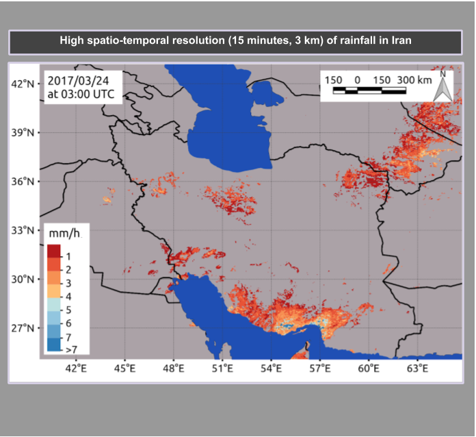
Estimating High Spatio-Temporal Resolution Rainfall from MSG1 and GPM IMERG Based on Machine Learning: Case Study of Iran

Faculty of Geography, Philipps-University of Marburg, 35032 Marburg, Germany
*
Author to whom correspondence should be addressed.
Remote Sens. 2019, 11(19), 2307; https://doi.org/10.3390/rs11192307
Submission received: 20 August 2019 / Revised: 24 September 2019 / Accepted: 1 October 2019 / Published: 3 October 2019
(This article belongs to the Section Atmospheric Remote Sensing)

Abstract

:
A new satellite-based technique for rainfall retrieval in high spatio-temporal resolution (3 km, 15 min) for Iran is presented. The algorithm is based on the infrared bands of the Meteosat Second Generation Spinning Enhanced Visible and Infrared Imager (MSG SEVIRI). Random forest models using microwave-only rainfall information of the Integrated Multi-SatEllite Retrieval for the Global Precipitation Measurement (GPM) (IMERG) product as a reference were developed to (i) delineate the rainfall area and (ii) to assign the rainfall rate. The method was validated against independent microwave-only GPM IMERG rainfall data not used for model training. Additionally, the new technique was validated against completely independent gauge station data. The validation results show a promising performance of the new rainfall retrieval technique, especially when compared to the GPM IMERG IR-only rainfall product. The standard verification scored an average Heidke Skill Score of 0.4 for rain area delineation and an average R between 0.1 and 0.7 for rainfall rate assignment, indicating uncertainties for the Lut Desert area and regions with high altitude gradients.

Graphical Abstract

1. Introduction

In semi-arid areas, the limited water availability from rainfall poses problems for agriculture and forestry (food and timber products), potable water supply, and energy production by hydro-power via dams. Climate change studies generally point to a reduction of rainfall, especially in semi-arid areas [1], which will most likely aggravate water scarcity in the future. This also holds for the arid and semi-arid regions of Iran, where the signal is strongly varying on the local scale [2,3,4,5,6]. To monitor changes in rainfall availability, accurate rainfall estimation at fine spatio-temporal resolution is important for water resource management. Thus, a dense ground observation network is also a precondition for proper hydrological modeling. Most arid and semi-arid regions are characterized by few precipitation gauge stations. Iran, where more than 60% of the country is composed of semi-arid regions, is facing two challenges: a strong information demand for water security on the one, confronted with a coarse network of operational rainfall gauges on the other. For this reason, in Iran but also in many other arid and semi-arid regions, satellite rainfall products are the only source providing area-wide precipitation observations in space and time, which renders them potentially attractive for hydrological management in ungauged basins [7]. However, their applicability in hydrology depends on the quality of the satellite data and the rainfall retrieval method used. Several products exist to derive rainfall from passive single or multi-spectral infrared (IR) sensors, passive microwave sensors, active radar instruments, and data fusion algorithms merging microwave and radar data with IR on geostationary satellites globally (e.g., TRMM [8]; CMORPH [8,9]; PERSIANN [10]).
Several studies in global rainfall-retrieval inter-comparison missions showed that the microwave and radar-based fusion systems are for the most part superior to purely passive IR techniques, and are particularly superior to rainfall-satellite-based models [11]. Data fusion algorithms increasingly include the GEO-IR (Geostationary Orbit, InfraRed) data, as well as the newest generation of global products, the Integrated Multi-SatEllite Retrieval (IMERG) for the Global Precipitation Measurement Mission (GPM) [12]. GPM was started in 2014 as a new generation of rainfall retrieval as a post-TRMM (Tropical Rainfall Measuring Mission) joint US–Japan mission. The GPM provides multi-channel, dual polarization passive microwave sensors and active scanning radar. The improvements of GPM in comparison to TRMM are: (i) The orbital inclination has been expanded from 35° to 65° to cover more important additional climate zones. (ii) Upgrading the precipitation radar to two frequencies, Ku band (13.6 GHz) and Ka-band (35.5 GHz). Anticipated advantages include a better sensitivity to light precipitation, and information on the particle size distribution in rain and snow. (iii) A GPM Microwave Imager (GMI) with a higher spectral resolution at frequencies of 10.65, 18.7, 23.8, 26.5, 89, 165.5, and 183.3 GHz [13]. Compared to TRMM, GMI was improved particularly by adding high-frequency channels (165.5 and 183.3 GHz) which lead to a better sensibility to light and solid precipitation [12]. However, the integration of GEO-IR data in IMERG is limited to only one thermal band at 10.7 µm, due to the difficulties in handling the data volume of multi-spectral GEO retrievals from various GEO platforms around the globe, and the limitation of visible data to daylight hours [12]. Despite the generally lower accuracy of an IR-based rainfall retrieval, the use of comprehensive IR data for rainfall retrieval—even in data fusion schemes—has been highly recommended based on the experience of the IPWG (International Precipitation Working Group) rainfall retrieval missions [14], particularly due to its high temporal resolution.
On the regional scale, however, regionally adapted algorithms using only passive IR data from geostationary orbit (GEO) revealed good accuracy, particularly when the full spectrum of available bands in combination with machine learning techniques were used [7,15,16,17,18,19,20]. The main advantage of GEO systems for rainfall retrieval is the high temporal resolution (15–30 min image repetition), which is lacking for passive microwave and radar sensors, perfectly matching the short-term characteristics of rainfall systems.
Concerning the incorporation of geostationary IR data in satellite-based rainfall retrieval algorithms, machine learning techniques are used extensively to identify relationships between predictor variables and rainfall estimates [10,19,21,22,23,24,25,26]. They offer a high potential in dealing with non-linear and complex relationships between the variables, but also with highly correlated predictor variables [20]. In recent years there has been considerable interest in the application of random forest (RF) in rainfall retrieval techniques [17,18,27,28]. RF is usable as a classification and regression technique and produces more accurate predictions than single-tree algorithms [29]. It offers a number of features compared to other machine learning algorithms that make it suitable for application in the remote sensing of rainfall: (i) It handles large data sets efficiently, while for example neural networks (NNETs) are not efficient in dealing with high-dimensional data without reducing the dimensions [30]. (ii) It has the potential to select predictors and define which are the most important. (iii) It has high accuracy in classification, while it is difficult to ensure classification accuracy with support vector machines (SVMs) for multi-class problems [30]. (iv) There is no need for complex data processing beforehand [30]. Islam et al. [27] classified rainfall areas from a satellite-borne passive microwave radiometer using RF classification. Kühnlein et al. [17] and Kühnlein et al. [18] modeled rainfall in Germany using RF, and trained MSG1 data with ground-based radar data. Both obtained promising results for the use of RF in rainfall retrieval. Min et al. [28] recently used Himawari-8 and GPM data to model rainfall using RF. Meyer et al. [20] compared different machine learning techniques (neural network, averaged neural network, support vector machine, and random forest) for satellite-based rainfall retrieval. They concluded that all of them are well suited for satellite-based rainfall retrieval, and none of them were significantly better than the others.
Several studies have applied the above-mentioned globally available data sets to Iran and compared the performance with gauge data. An intercomparison of PERSIANN and TRMM-based products showed the superior performance of the TRMM-based products, but still found some underestimations and bias problems [31,32]. PODs (probabilities of detection) of 40% and less were achieved, depending on the region. A bias correction could be applied to slightly improve the quantitative precipitation assessment results [33]. In a recent study in Iran, it could be shown that the new IMERG product outperformed TRMM-based products and ERA-Interim reanalysis rainfall particularly for orographic, stratiform, and heavy precipitation [34]. However, the authors stressed that the occurrence of over- and underestimations indicated a remaining challenge of reliable satellite-based rainfall retrieval in Iran. They emphasized that the limited spatio-temporal coverage of data in the algorithm (e.g., limited MW/radar and operational rain gauge network) in comparison to the complex topography, as well as the high spatio-temporal variability of rainfall in the semi-arid area, were most likely the main reason for the obtained inaccuracies.
Thus, the main aim of the current study was to combine the advantages of second-generation GEO systems and the new IMERG product in order to develop a regionally adapted rainfall retrieval scheme with high temporal resolution based on a machine learning algorithm. In detail, we used the Meteosat Second Generation (MSG) SEVIRI (Spinning Enhanced Visible and InfraRed Imager) multispectral radiances and RF algorithm, and the RF model was regionally trained using passive microwave (sounder and imager) rainfall from GPM IMERG. However, RF model training was restricted to areas and time slots where the best microwave quality of IMERG was available. The area validation of the applied RF model rainfall products was also conducted for pixels from microwave-based IMERG, but for pixels that were independent from the model training data set. The same was true for RF model product point validations with available weather station data, which were not used in the generation of the IMERG product and were thus completely independent.

2. Data and Method

This section firstly describes the general rainfall retrieval method (Section 2.1). Then, we give an overview of the data sets that were used (Section 2.2, Section 2.3 and Section 2.4). After that, we describe the RF model generation and the final rainfall retrieval model in detail (Section 2.5, Section 2.6, Section 2.7 and Section 2.8).

2.1. Rainfall Retrieval Development

The aim of this study was to develop a new satellite rainfall product by combining the available microwave-based GPM IMERG rainfall information, which has the advantage of accurate rainfall estimates, with the high spatio-temporal resolution of MSG. Toward this end, the new rainfall retrieval algorithm is based on the IR bands of MSG1 and trained with the best microwave-quality data of the IMERG product (i.e., microwave-based IMERG). The general workflow is depicted in Figure 1. The basic principle of this algorithm is first to delineate the rainfall area within cloudy regions with an RF classification. In the second step, this information is then used to estimate the rainfall amount with a RF regression model. These two steps are implemented following previous studies which showed promising results for central Europe and other areas [17,19,28,35].
The work flow of the development of the new rainfall retrieval method is depicted in Figure 1. First, the RF model predictors had to be matched to a spatio-temporal homogenous data set: (i) MSG1 SEVIRI IR-channels, (ii) its spatial texture features, (iii) channel differences, and (iv) ancillary geo-information data were processed and collected for areas and time slots that were also covered by the microwave-based IMERG products (rain area and rate) (Section 2.5) (Figure 1 left). The data were used to train and develop the two RF-models: (i) The RF classification to delineate rainy and no-rain cloud areas (Figure 1 left, in Section 3.2.1), and (ii) the RF regression model to estimate rainfall (Figure 1 right, in Section 3.2.2). The training of rainfall area delineation and rainfall estimate assignment were done independently.
Both best-trained RF-models were applied to the study area (Figure 2) and the resulting rain area/amounts were validated against an independent microwave-only IMERG dataset from regions which were not used during the training process (see Section 3.2.3). Finally, the RF-models were applied to the whole time period of available MSG-SEVIRI data in the original spatial and temporal resolution (15 min) of MSG1. Because the first validation was conducted with IMERG (even with pixels not involved in training), a second, completely independent, validation of the RF rainfall estimate was conducted against gauge stations which were neither part of the IMERG product nor used for model training (see Section 3.2.4). Note that the term “feature” that is generally used in RF models has the same meaning as “predictor”.

2.2. Predictor Dataset

The rainfall retrieval model presented here uses the IR wavelengths (all bands between 3.9 and 14 μ m) from MSG1 SEVIRI. Processing was performed using software developed by Drönner et al. (2019) [36]. In addition to the MSG1 data, the cloud mask (CLM) product [37], which is mainly based on the MSG SEVIRI data, was used to outline the domain for cloudy pixels that was used for training the RF models. Several IR bands from MSG1 SEVIRI and different band combinations (DIF) that have been proven to improve the rainfall estimation by satellites were included as predictors [18,35]. This also holds for the spatial variability in the spectral bands and DIFs [38,39,40,41], where respective metrics were also included as predictors for the RF models. Different texture features were calculated from a 3 × 3 pixel moving window approach: For the single bands (i) variograms (VARs), (ii) madograms (MADs), (iii) rodograms (RODs) and (iv) cross-variograms (CVs), as well as (v) pseudo cross-variograms (PCs) of each channel combination [39].
Besides that, an increasing number of studies found that mountainous regions in semi-arid areas are one of the great challenges regarding rainfall satellite retrievals both, in IR and microwave products. This is due to the high weather variability [42] related to the topographic forcing of rainfall formation and decay. Similar conclusions are also drawn for low and mid-elevation areas of Iran [32,33,43,44,45]. Due to the importance of topography for rain formation, (i) terrain elevation (ELV), (ii) the Topographic Position Index (TPI), (iii) the Topographic Roughness Index (TRI), (iv) slope and (v) aspect were also added as predictors to the training data set. The predictors are derived from the Global 30 Arc-Second Elevation DEM [46]. The list of predictors that are used in this study is depicted in Table 1.

2.3. GPM IMERG Training and Validation Data

To train and validate the RF model developments for rain area and amount against the predictors (Section 2.2, Table 1), we used the microwave-based rainfall estimates from the IMERG product only. IMERG is a level-3 gridded precipitation product from the GPM constellation. It calibrates, merges, and interpolates the measurements from a network of satellites, together with a precipitation gauge analysis every half hour in 0.1° spatial resolution [47]. IMERG is designed to use as many low Earth orbit (LEO) satellites as possible to compensate for the limitations in available satellite microwave precipitation estimates as effectively as possible, in conjunction with IR estimates from GEO satellites. IMERG has three runs to provide different user requirements for latency and accuracy. This study focuses on the final run of 30-min IMERG Version 05 (IMERG-V05), using the gauge-adjusted estimates from 12 months of data between February 2017 and February 2018. Since IMERG-V05, the quality index (QI) is included as a new variable with half-hourly resolution in the metadata provided by NASA [47]. The QI is a metric concerning the relative skill of the temporally fluctuating mix of different passive-microwave-and IR-based rainfall estimates in half-hourly IMERG products. Additionally, the time of the overpass of each microwave swath in each scene is also available under the flag HQ observation. For the rainfall retrieval model development, the microwave-based pixels from the multi-satellite precipitation estimates with the gauge calibration sub-dataset of IMERG was used for training and validation. The final compiled data set (including predictor and target variable dataset) was selected on cloudy pixels, where the high-quality IMERG data was available (QI > 90%). Seventy percent of the compiled dataset in each scene was randomly selected as the training dataset, and thirty percent of the remaining pixels in the scene were selected for validation.

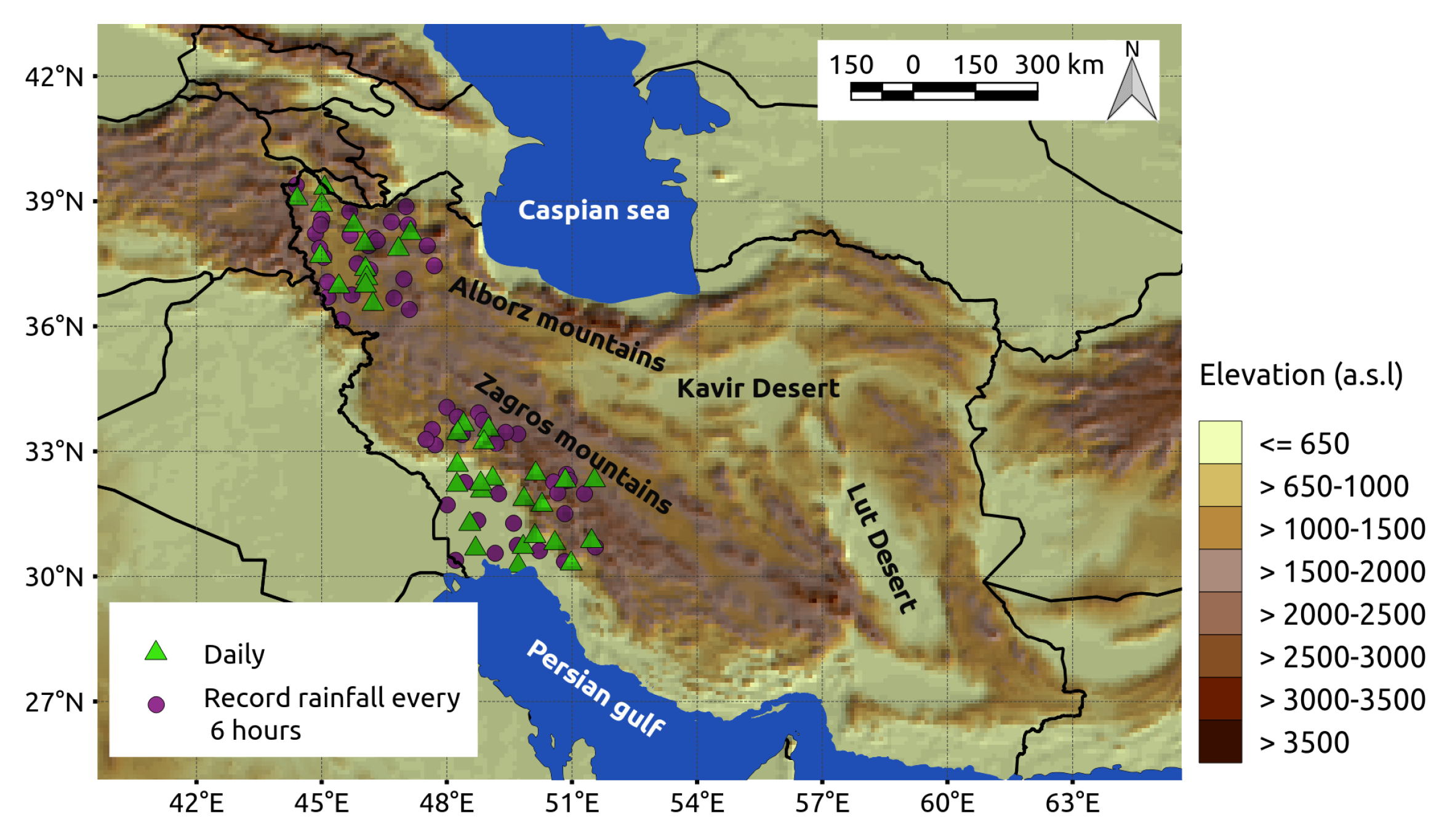
2.4. Station Data for Independent Point Validation

Precipitation gauge data for February 2017 till January 2018 were obtained from the Islamic Republic of Iran Meteorological Organization (IRIMO) for Khouzestan and Urmia provinces. These data are independent of the gauges used for the IMERG calibration, and are in two different recorded time steps. One group consists of the rainfall in every 6 hours, and another group records data at a daily scale. They were complemented by the data derived from the Urmia Lake Restoration Program (ULRP.sharif.ir/en). The data from both organizations underwent quality checks before they were delivered. The distribution of rainfall gauge stations used in this study is shown in Figure 2.

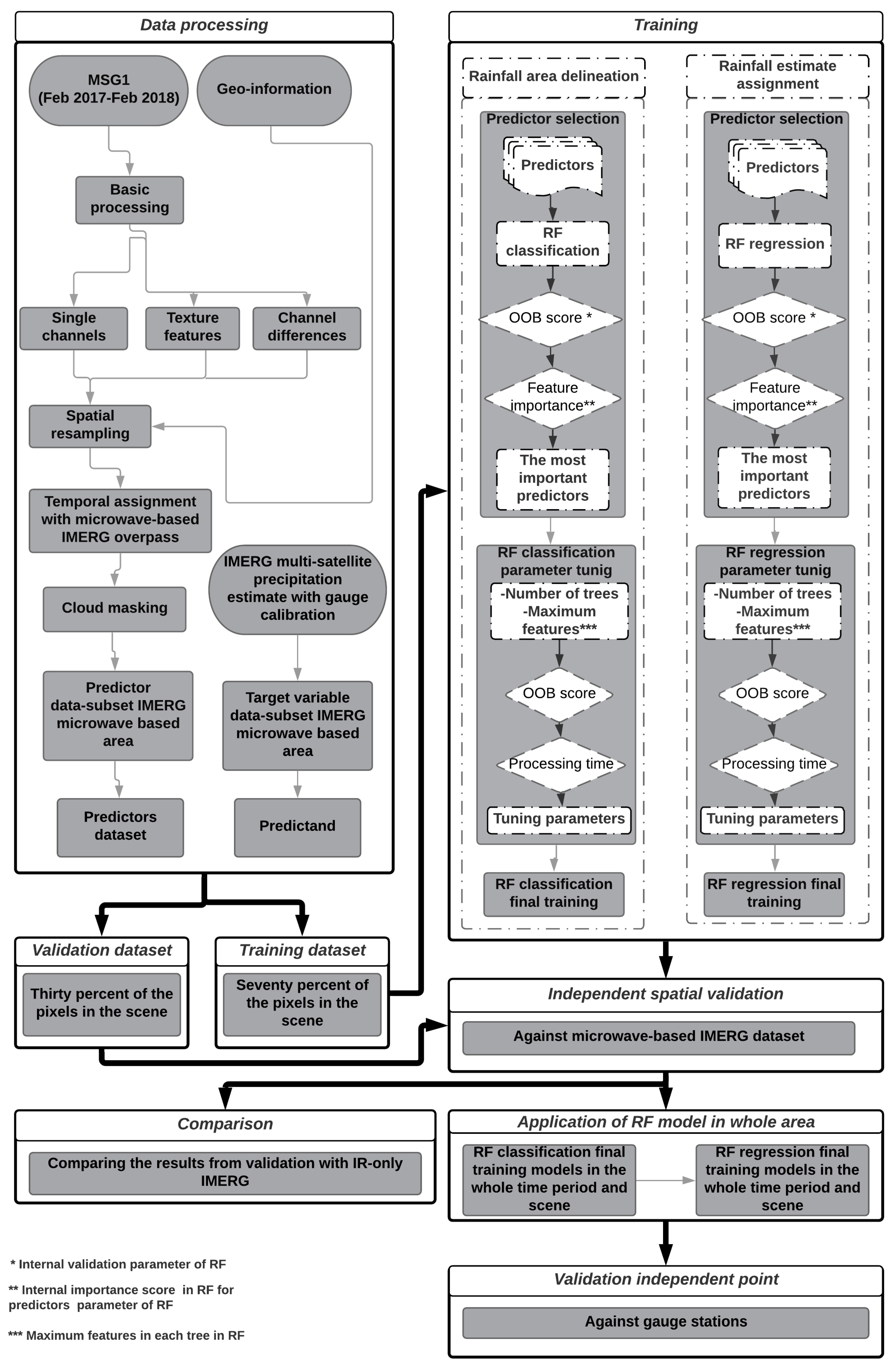
2.5. Data Processing

With reference to Figure 1, our new rainfall retrieval was done in five steps. The first step included data processing. The different temporal and spatial characteristics of MSG1 data (15 min; 3 × 3 km 2 at the sub-satellite point) and IMERG (30 min; 11 × 11 km 2 ) were addressed to ensure pixel matching between Meteosat, geo-information, CLM, and IMERG data. Thus, MSG1, CLM, and geo-information data were projected and resampled (average) to the spatial resolution of IMERG. Because MSG feature and IMERG training data can temporally deviate by hours, the temporal overlap of <7 min was used to ensure proper comparability between both data groups. A seven-minute threshold was determined as an average acquisition time between the MSG1 scan in Iran (occurring between minutes 7 and 10 for each full disk scan of Earth with MSG1) and HQ observation time overpass of IMERG. Then, the QI was used to mask out the microwave-based-only pixels from the entire IMERG data set. Finally, the CLM product was used to limit the training data sets to areas where precipitation is generally possible, as indicated by cloudiness. However, it should be stressed that for the training of the RF models, only pixels with rain rates higher than 0.2 mm/h were considered as rainy, warranting reliable information on rainfall in IMERG [12,48]. This threshold was chosen due to the estimated minimum detectable rain rates of the Ka- and Ku-band radars [49]. After the last step of preprocessing, a consistent data set for training and validation of the RF models was compiled.

2.6. Model Training and Tuning

The first step for the training of the RF models was the selection of the most important predictors. This involved a reduction to the best-performing predictor sets out of the initial feature data space presented in Appendix A. Here, the predictor selection was conducted by applying a recursive feature elimination (RFE) for each month of the training dataset. RFE started with all of the initial 121 predictors and removed the least significant ones using the feature importance metrics of the RF methods [29]. In each step of this iterative RFE procedure, the model quality was calculated using the out-of-bag (OOB) score. The OOB score was measured during model fitting based on the left out data (one-third of the observations) for each tree in the RF [50,51]. The set of predictors with the best average ranking (sorted based on feature importance) that reached the highest OOB score was filtered from the original set of 121 (Appendix A) for each month and used as the training input for the final RF models.
With the completion of the RFE step, we iteratively tuned the hyperparameters, including the total number of decision trees and the number of input features (n) used at each node to get the optimal setting for the RF classification and regression model in each month, following the successful approach of different studies [18,28,39] for RF model training. For each parameter set, RF models were trained based on the tuning data set and the OOB score was calculated. In addition, the balance parameter in the RF package “compute sample weight” from Scikit-learn 0.20.2 [52] in Python 2.7 was also implemented for both RF regression and classification.
To save computation time for RFE and parameter tuning, we randomly selected the data from the whole training dataset. For rainfall area delineation, 10,000 pixels from the available training pixels in the month were randomly selected including 2000 rainy and 8000 cloudy pixels. For the rainfall estimate RFE parameter tuning, we randomly selected 2000 rainy pixels in each month. It should be stressed that the distribution of rainfall rate within a month varies and RF regression models are not able to predict unbalanced datasets [28]. Therefore, in order to increase the rainfall prediction accuracy, the balanced sampling technique [28] was used for RFE and parameter tuning of the RF regression. For each month, the rainfall rate was classified with the range of 1 mm/h and the probability of occurrence of every rain rate class was calculated for each tuning data set. The class with the average probability of occurrence (APO) was selected and the new sample stemmed from the original sample by simply decreasing the low rain rate sample to the APO. Fifty runs were performed for both RFE and parameter tuning to produce fifty series of a randomly selected pixel for each month. Differences between these fifty realizations reflected the whole range of internal variability of the microwave-based IMERG in the region and in the month.

2.7. Application of the Rainfall Retrieval Model

After the successful adjustment of the microwave-based IMERG models for rainfall area delineation and rainfall rate assignment, each 15-min image from MSG1 was then processed using the best trained models at the microwave-based IMERG resolution of 11 km to generate rainfall estimates with high spatio-temporal resolution. Since the microwave-based IMERG models are limited in time, the range of the available models in a day differs between 3 and 25, depending on the time of year. To generate the rainfall estimates in MSG1 generic resolution, we applied the models in the scene of the same time slot, and the following scenes until the next microwave-based IMERG RF model was available. In cases where the previous model belonged to the last months, the first model in the upcoming months was applied for the scenes, where a model was available.

2.8. Validation

In order to assess the model performances, two different validation strategies were employed:
  • The performances of the trained rainfall area delineation and rainfall rate assignment models were investigated on a scene-by-scene basis, using 30% of the independent pixels from each scene.
  • The overall performance of the rainfall area delineation and rainfall rate assignment was investigated against gauge station after application of the model in the whole study area for the whole time period.
First, the performance of the rainfall area delineation and rainfall rate assignment on a scene-by-scene routine was investigated after training the model. By extracting the data pairs of the validation data sets on a pixel basis, a total of 287,750 pairs of RF classification/regression and microwave-based IMERG were made available at a half-hourly resolution for validation. Then, in the next step, the performances of RF models were compared in the same location with sub-dataset IR-only IMERG. With the latter analysis, we could reveal if the new multispectral GEO retrievals were superior to the IR-only IMERG solution.
For the validation of rainfall area delineation, all pixels from the validation dataset that were classified as cloudy by CLM were considered. First, we calculated the crosstables for the RF classification and IR-only IMERG using RF-modeled pixel values in comparison to the microwave-based IMERG as reference. The hits (H), misses (M), false alarms (F) and correct negatives (C) between each pair of the dataset were calculated. A hit was considered when both the reference and the estimate pixels were raining; a miss was indicated when the reference was raining but the estimate was not; a false alarm occurred when the reference was not raining but the estimate was; and a correct negative was when both the reference and the estimate were not raining. From the hits, misses, false alarms, and correct negatives, we calculated the average half-hourly probability of detection (POD), false alarm ratio (FAR), and Heike skill score (HSS) as validation metrics. The detailed equations and the range of these metrics are shown in Table 2.
The POD indicates the fraction of correctly modeled rain pixels. A perfect score is 1. The FAR gives the percentage of estimated pixels incorrectly estimated as rain. A perfect score is 0, implying that the RF classification or the IR-only IMERG never estimate a qualified precipitation rate when the microwave-based IMERG indicates no precipitation. The HSS is a metric for the general model performance that quantifies whether the estimate is worse or better than the microwave-based IMERG. A perfect score is 1. To evaluate the ability of the RF regression model to estimate rainfall, the correlation between the reference dataset and the estimated half-hourly rainfall was calculated using the correlation coefficient (R). Root mean square error (RMSE) and the mean absolute error (MAE) were also calculated. All rainy pixels from microwave-based IMERG were used for the validation of rainfall estimates.

3. Results

3.1. Training Results

In each of these steps, first we selected the most important features (results in Section 3.1.1), then tuned the hyperparameters for the model development (results in Section 3.1.2), and finally the RF models were applied. Please note that due to the low availability of rainy pixels in June, training and validation was not possible for this month.

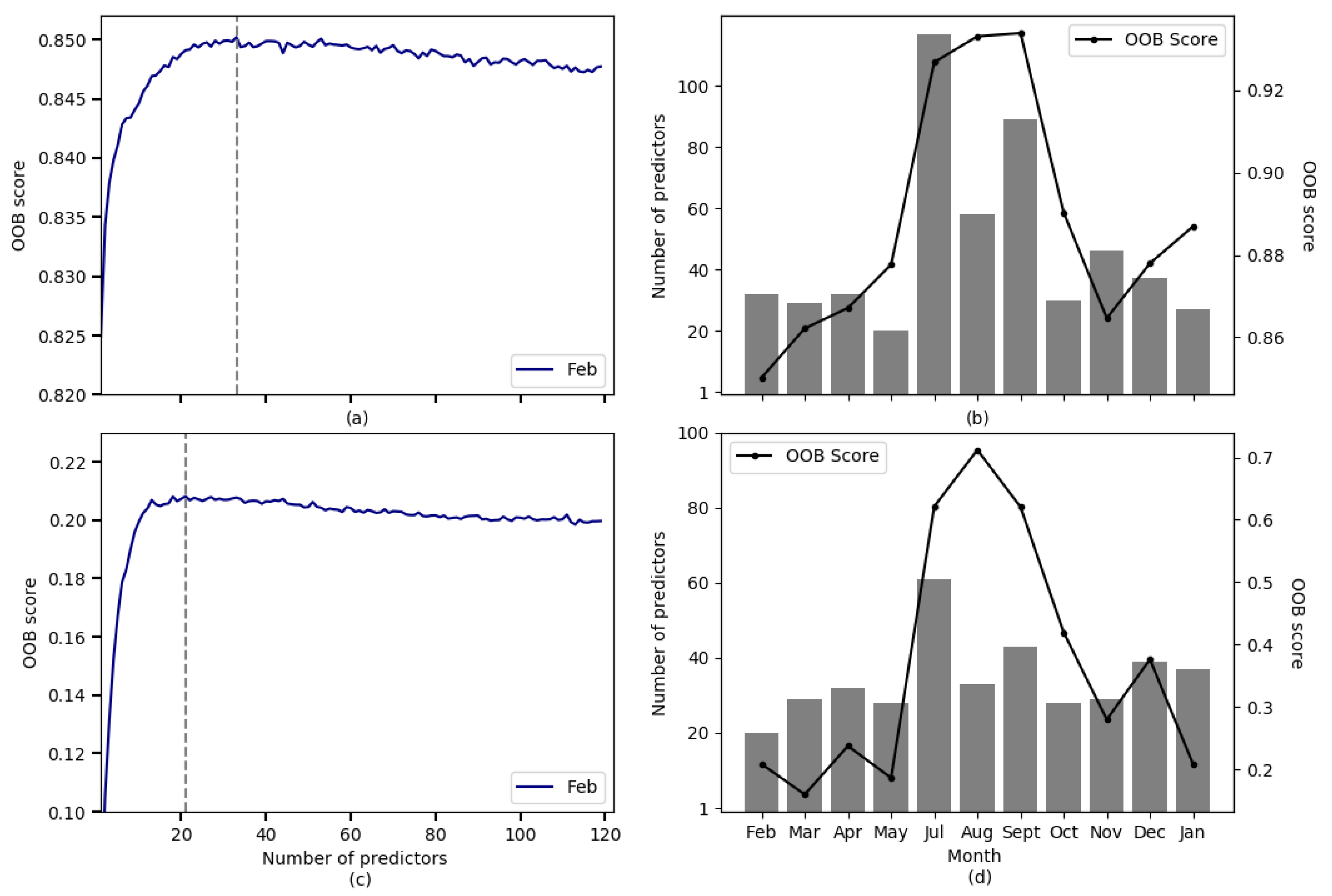
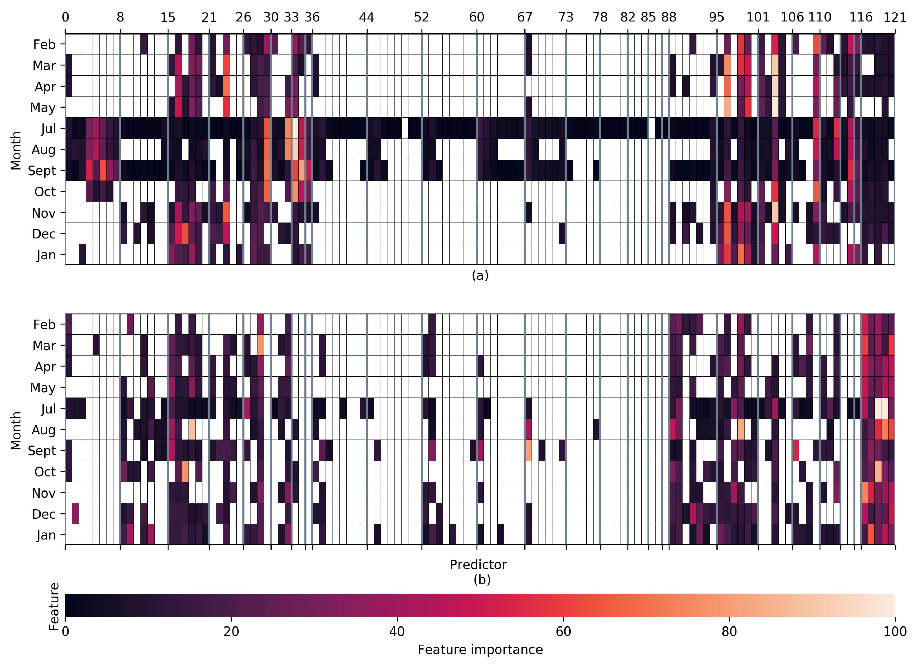
3.1.1. Results of Recursive Feature Elimination

RFE results are depicted in Figure 3.
In Figure 3a,c, the average RF classification and regression in February are respectively shown as examples. The RF classifications for rain are delineated showeing the best model performance with an OOB score of 0.85 at 33 remaining features. The performance of the RF regression model for rain amount was less pronounced, with the best model performance at an OOB score of around 0.2 and 20 remaining features. In both models, having more features from the set resulted in a worse result. The same process was performed in each month for the whole time period, and the number of features that led to the best RF model performances was defined. The optimum number of features is shown in Figure 3b for RF classification and Figure 3d for RF regression with respective OOB scores for the study period. The number of features of RF classification in summer (July, August, September) increased significantly. However, July, August, and September showed the highest OOB scores in both RF classification and RF regression.
In the next step, feature importance was used to define the most important predictors considering the optimum number of already-defined predictors.
Figure 4 illustrates the selected predictors and the feature importance for both RF classification and RF regression. In both models, the combination of CV for the IR 8.7 (features 79–82), CV for IR 9.7 (features 83–85), CV for IR 10.8 (features 86 and 87), and CV for IR 12.0 (feature 88) did not play roles at all, except for July which showed greater complexity in the rainfall area delineation due to the lower number of cloudy pixels. This was also true for all MADs (features 45–52). The single channel of IR 10.8 had a relatively high feature importance in the warm seasons for the RF classification. This channel provides information about the cloud-top temperature, and thus the cloud height [18].
Figure 4b shows that the terrain features were identified as having the highest impact in modeling the rainfall amount. Besides that, for both rainfall delineation and rainfall assignment, the Δ T 8.7–10.8 (features 28) and Δ T 10.8–12.0 (features 34) were mostly selected in each month. These band combinations have been proven to provide information about the cloud water path [53] and thus improve rainfall retrieval models [18]. In both models, one or more of the combination of band WV 6.2 with WV 7.3, IR 8.7, IR 9.7, IR 10.8, IR 12.0, and IR 13.4 (features 16–21) was selected in each month. The differences between the brightness temperature in water vapor and IR channels were shown to correspond to deep convective clouds with heavy rainfall [54,55,56]. These band combinations have been proven to provide information about the cloud water path [53] and thus improve rainfall retrieval models [18]. In both models, one or more of the combination of band WV 6.2 with WV 7.3, IR 8.7, IR 9.7, IR 10.8, IR 12.0, and IR 13.4 (features 16–21) was selected in each month. The differences between the brightness temperature in water vapor and IR channels were shown to correspond to deep convective clouds with heavy rainfall [54,55,56].

3.1.2. Parameter Tuning

For RF model training, we tuned the parameters iteratively in order to find an optimal model with regard to the number of decision trees and the number of input features (n).
The sample parameter tuning for February is shown as an example in Figure 5. The model performance of rain area and rain estimate assignment increased significantly in the beginning until the number of decision trees reached 250. Beyond this, the increase slowed down. This trend was almost the same for each month of the time period. The OOB score values were almost the same when more features were considered at the nodes and the number of trees increased. As a compromise between prediction accuracy and processing time, a cut-off was made at a number of trees of 250 and n was set to default in both final RF models for the rainfall area delineation ( Number of features ) and rainfall rate assignment (Number of features/3).

3.2. Accuracy of Rain Area and Rainfall Retrieval

The validations of the RF models for rainfall area delineation and rainfall rate assignment were conducted independently. In each step, the results of the model were compared pixelwise with the microwave-based IMERG. Furthermore, the results were compared to IR-only IMERG. In order to compare the RF model results with IR-only IMERG, the validation scores for IR-only IMERG were also calculated.

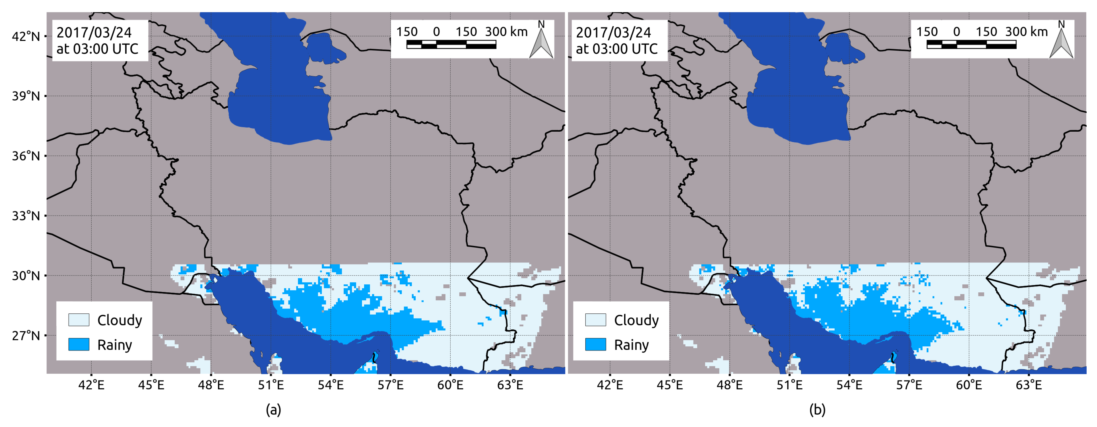
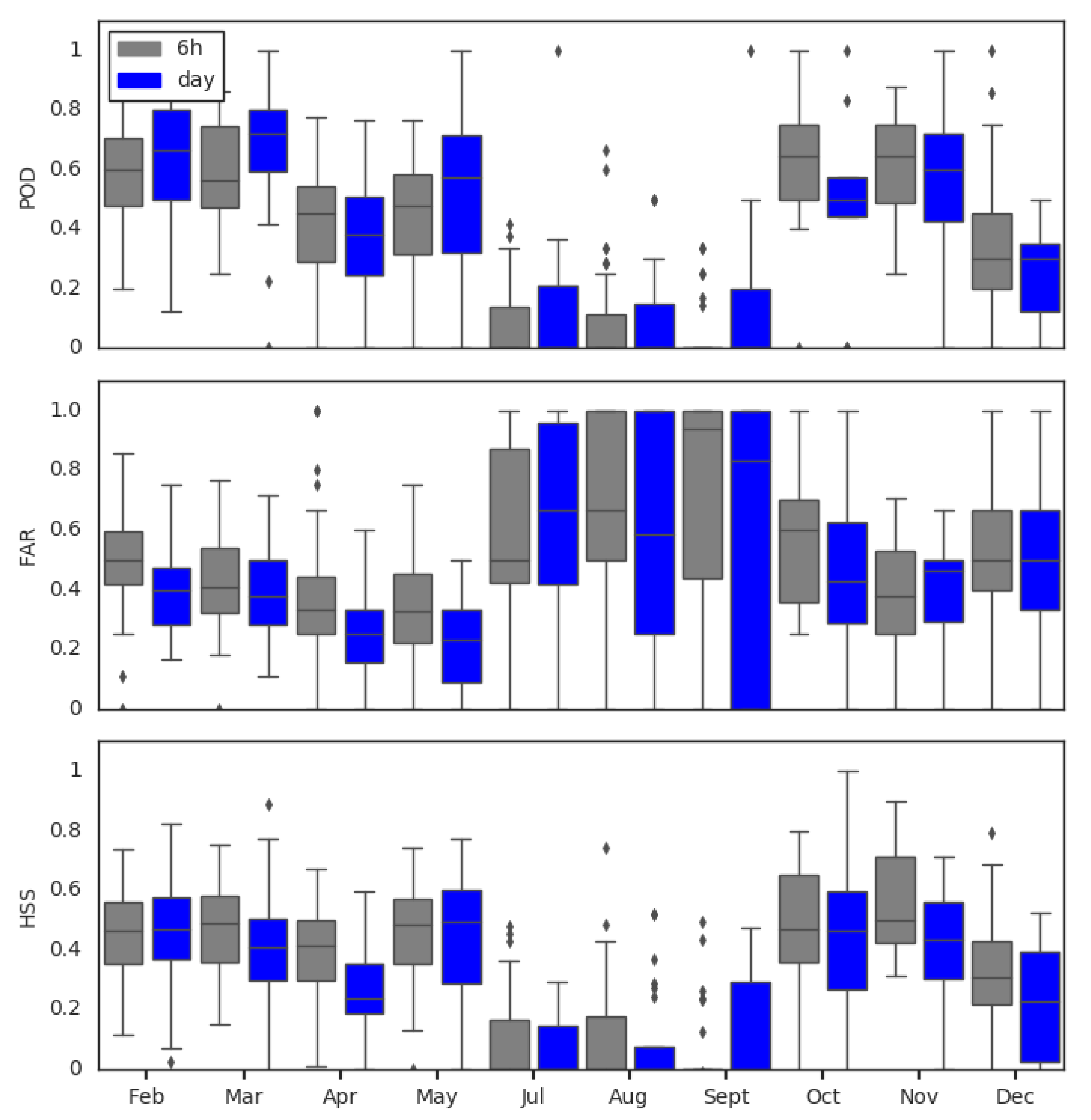
3.2.1. Rainfall Area Delineation

The validation scores for rain area delineation were calculated on a pixel basis for each scene. As the ratio of the number of non-rainy pixels to rainy pixels was quite high, we had an unbalanced dataset. An unbalanced dataset in rainfall delineation using RF classification was shown to influence the model accuracy [18,28]. As suggested by several authors [18,28], the balanced sampling technique was used to improve model performance. The number of non-rainfall but cloudy pixels that normally define the majority class were randomly downsampled in order to equal the number of majority and minority classes. This technique was applied in two sample weeks from July and August in the training dataset. We defined different scenarios to conduct diverse sensitivity studies. Table 3 summarizes the statistics on the verification scores of RF classification with different ratios of majority versus minority class.
The HSS and FAR showed better model performance in both months in Scenario-3. Therefore, we implemented the Scenario-3 relation between cloudy and rainy pixels for the whole study period for rainfall area delineation.
The verification scores for rain area delineation are presented in Figure 6. Given that the evaluation was done on the number of microwave-based IMERG scenes, results are summarized as box-and-whiskers plots and are shown for both the newly developed RF model and the to-date implemented IR-only IMERG procedure.
Figure 7 shows an example of the spatial distribution of the RF prediction of the rain area, showing the rain area detected by RF classification (Figure 7b) in comparison to the microwave-based IMERG (Figure 7a). The RF classification showed a good agreement with the observed rain areas.

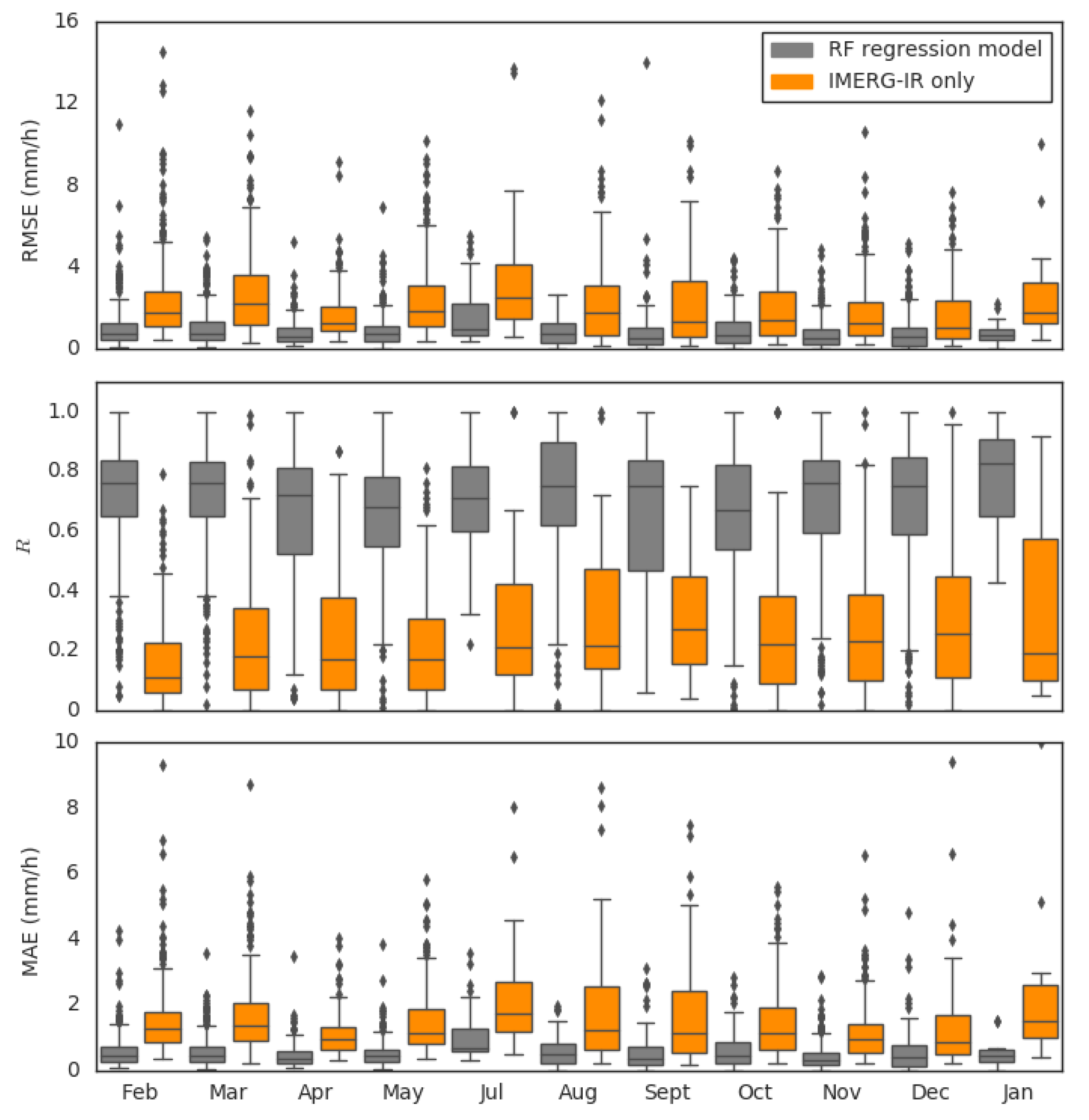
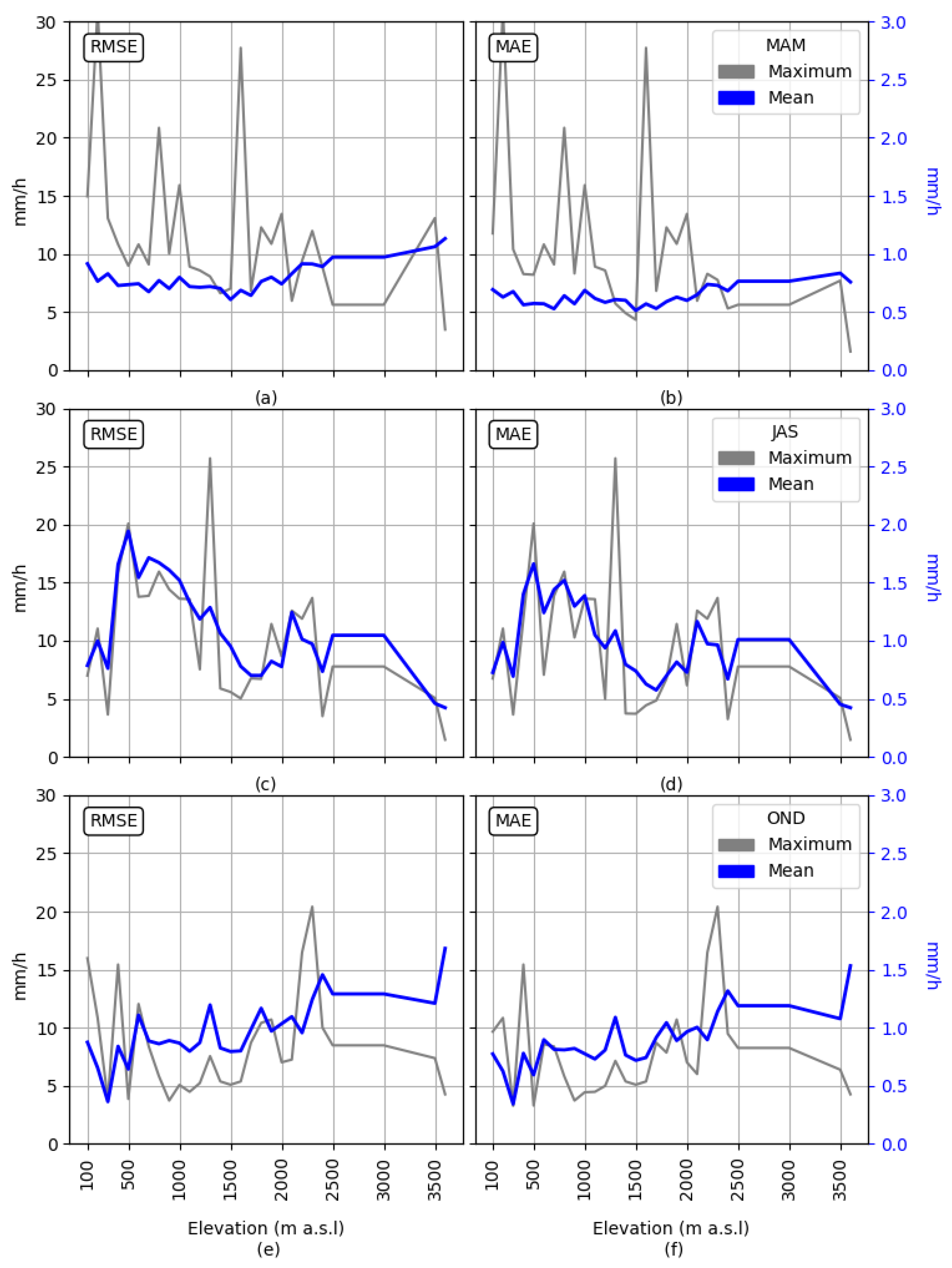
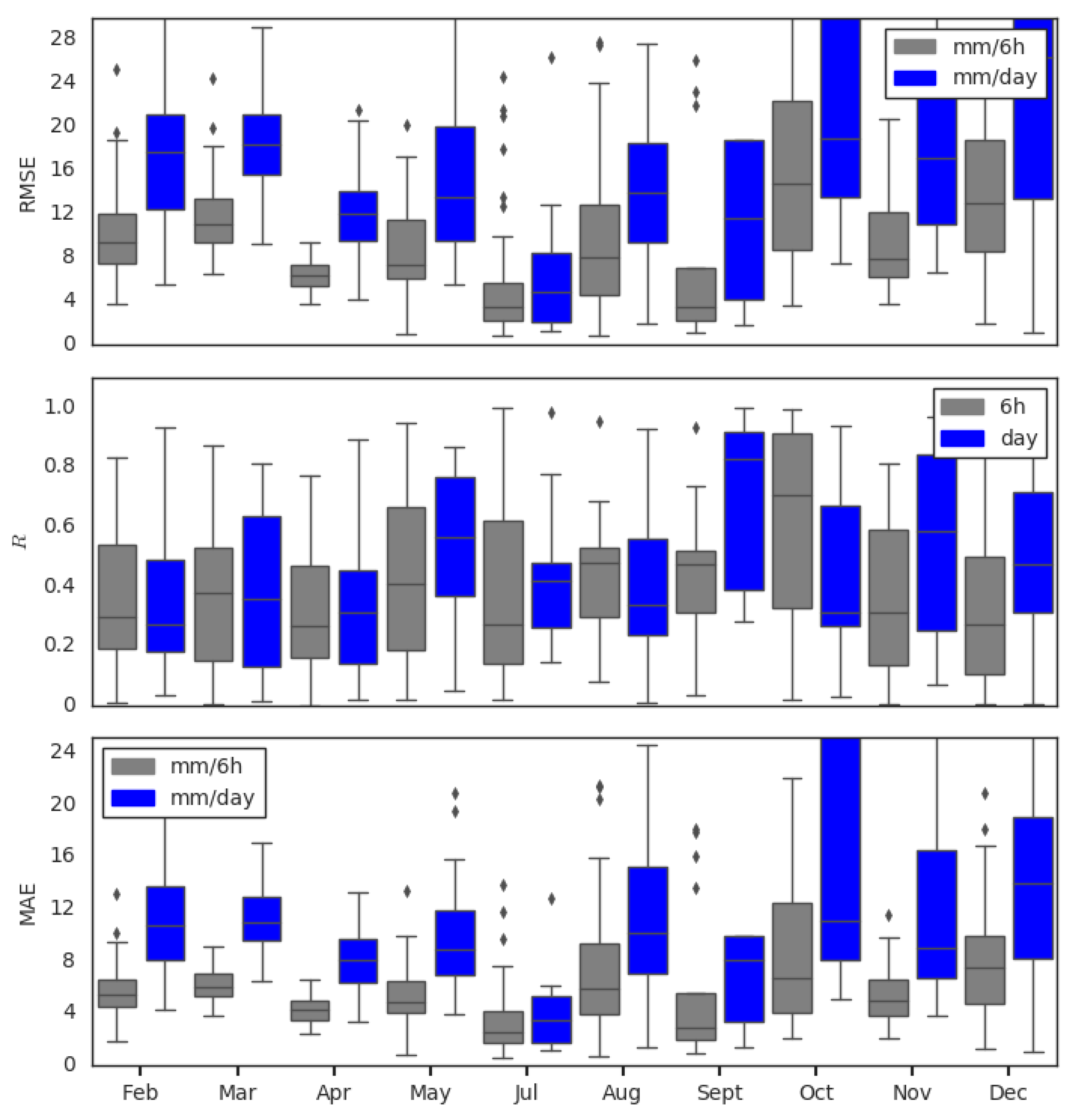
3.2.2. Rainfall Rate Assessment

The evaluation metrics for rainfall rate assessment are shown in Figure 8. The comparison of the RF regression rainfall assessment and microwave-based IMERG, as well as IR-only IMERG retrievals, was conducted for 1595 scenes of precipitation events in the study period. The number of pixel pairs available for the time period was 287,750.
Figure 8 also reveals the occasional high RMSE and MAE between the RF regression and microwave-based IMERG retrievals in almost all months, which are shown as outliers.
As an example, Figure 9 shows the microwave-based IMERG (Figure 9a) and the newly developed rain rate retrieval (Figure 9b) for 24 March 2017 at night.

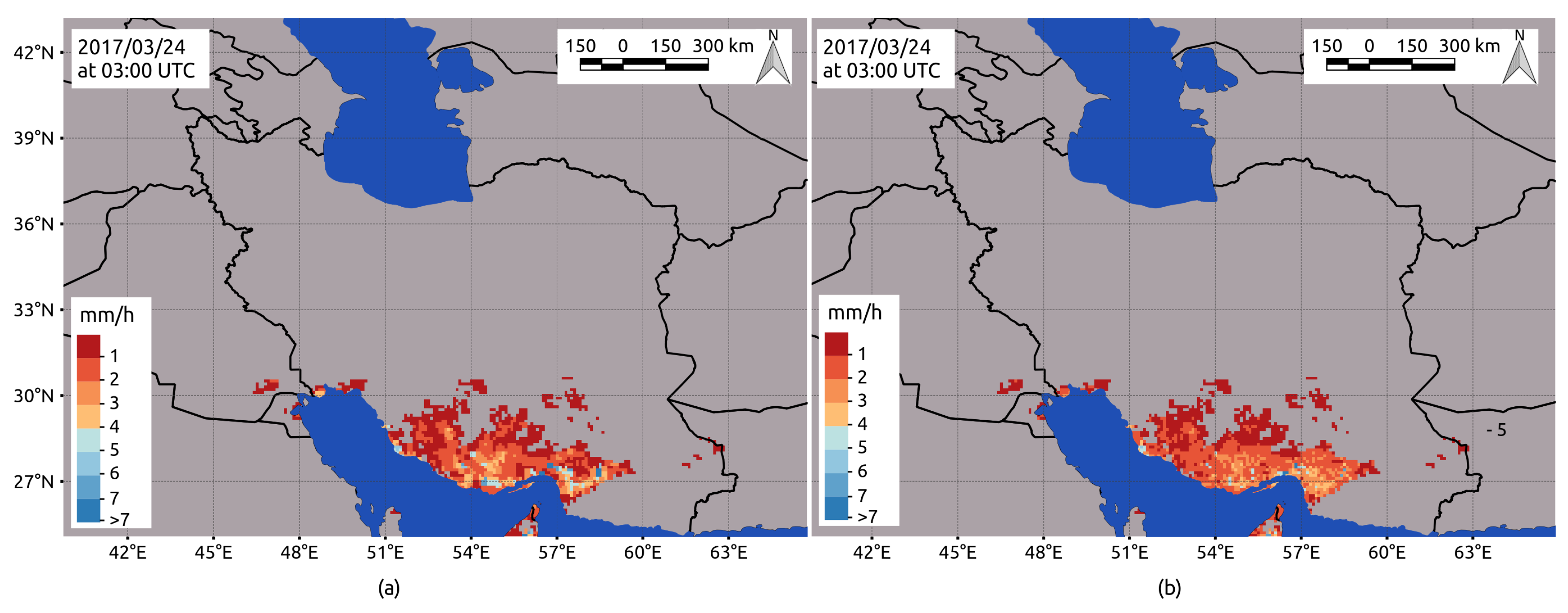
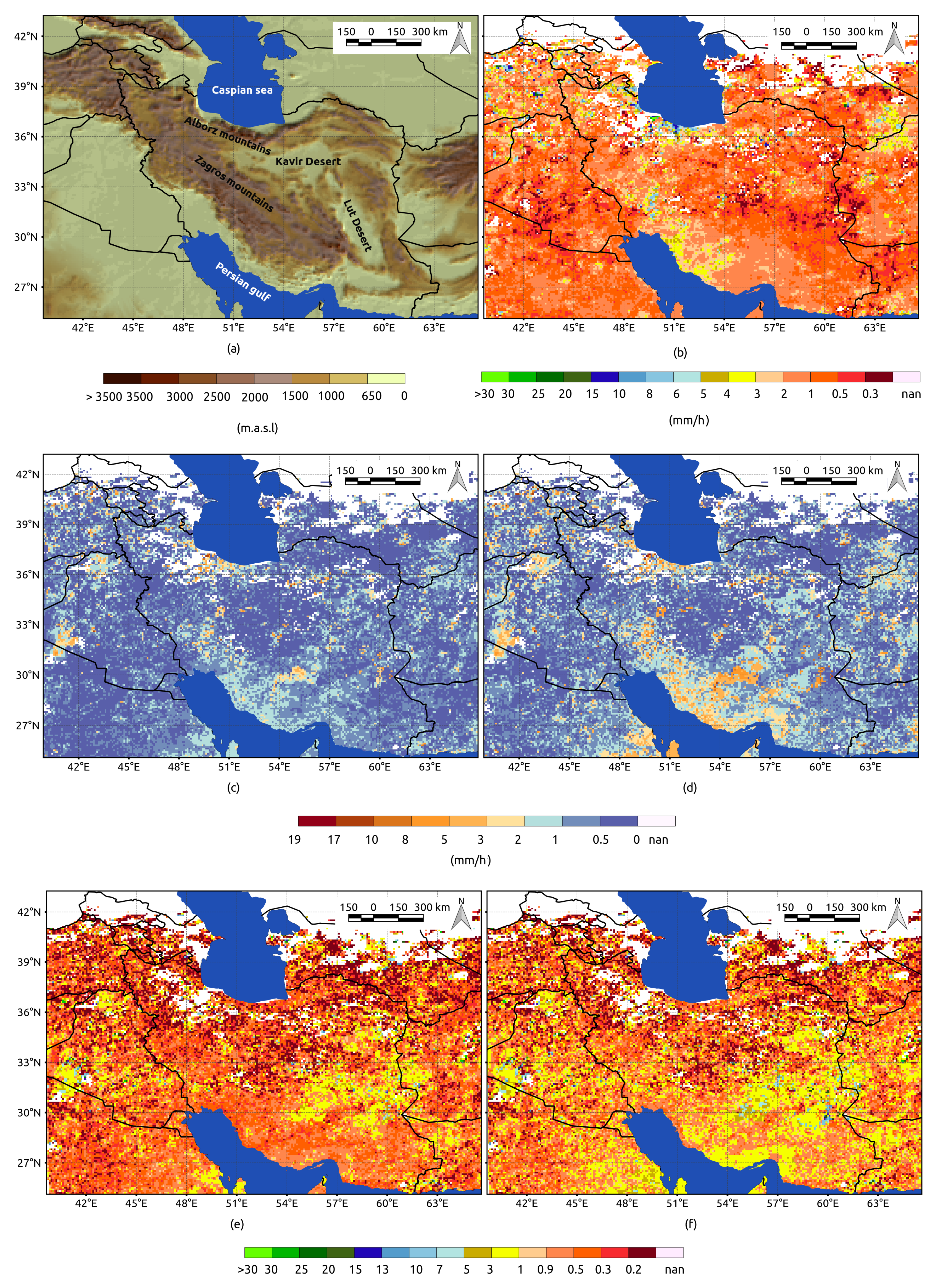
3.2.3. Overall Performance of the Merged Rainfall Retrieval Model (Rain Area and Rate)

To assess the overall performance of the rainfall retrieval developed in this study, the RF classification and RF regression was combined and the finally merged product (rain area and rate) was evaluated (Figure 10). Thus, all errors from both RF models were accumulated in the final spatio-temporal rainfall estimate. The validation of the model was conducted only for areas that were classified as rainy in the microwave-based IMERG product.
The outliers of RMSE and MAE increased compared to the rain estimate validation in Section 3.2.2. The high RMSE and MAE could be related to the number of pixels in the calibration dataset, especially for April, September, May, July, October, December, and January. This relationship is shown in Figure 11. The higher RMSE and MAE values were normally shown for scenes in months with fewer rainy pixels in the calibration dataset. However, other factors (e.g., the complexity of the rainfall rate, influenced by parameters like elevation diversity in the scene) may have led to uncertainties in the RF model.
Figure 12 gives an overview of the model performance along with the altitude during different time periods of the study period. The study period was divided into two rainy seasons (i.e., March, April, May (MAM) and October, November, December (OND)) and one dry season (i.e., July, August, September (JAS)). Terrain elevations around 200–500 m showed relatively high maximum RMSE and MAE values for all time periods. These heights can mostly be found in the Lut Desert and along the coast of the Caspian Sea (Figure 12a).
Figure 13c,d indicates the spatial distribution of the MAE and RMSE, and Figure 13e,f shows the spatial distribution of the MAE and RMSE relative to the average rainfall rate for the whole study period (February 2017 to February 2018) in the study region.
The average RMSE and MAE (Figure 13c,d) showed relatively higher values in the Zagros mountainous region (~0.5–6 mm/h for MAE and ~0.4–16 mm/h) and Alborz mountainous range (0.5–8 mm/h for MAE and ~0.5–12 mm/h). Meanwhile, in Figure 13c,d the relative RMSE and MAE in the mountainous region show some uncertainties in the area between 50E, 32N and 51E, 33N with the value of ~18.67 and in the connection zone between Zagros and Alborz in the north-west of the country with values between ~0.5 and 25. The RMSE, MAE, and rainfall rate near the coast of Caspian Sea, at the northern slopes of Alborz mountains (Figure 13c,d) indicated higher errors (~20 mm/h). In the Kavir Desert in the center of the country, the RMSE and MAE of the RF model were estimated as ~0.1–16 mm/h.

3.2.4. Comparison to Gauge Stations

To validate the RF model performance against a completely independent dataset, we used gauge stations from Iran (Figure 1) as a reference. In this step, we applied the model to the original spatial and temporal resolution of MSG-1 (3 km, 15 min) for the whole study period, and the results were compared to the available rain gauges. The 15-min rainfall rates were added up to 6 h and 24 h, respectively. For comparison, the pixel values of the corresponding station coordinates were extracted.
The overall performances of the model against gauge are shown in Figure 14 and Figure 15. During our research period, the available gauge stations for our study were 45 synoptic stations in the temporal resolution of 6 h and 32 stations with daily resolution. Our results indicate the expected seasonal behavior for rain area validation scores. During the dry summer (JAS), the RF model performed worst with a POD less than 0.2, FAR more than 0.6, and poor performance, as indicated by the low HSS. In the rest of the year, the average HSS was ~0.3–0.55 and ~0.25–0.55 per 6-h and per day, respectively. The best POD ranged between 30% to 70% in winter, autumn, and spring. The average daily RMSE was around 16 mm and the average daily MAE was around 10 mm depending on the month. The overall range of R was between ~0.17 and 0.8 for all months except JAS.

4. Discussion

4.1. Performance of Rain Area and Rainfall Retrieval Model

Feature elimination and parameter tuning procedures were carried out to determine the final input feature set. The results of the feature selection in RF regression (rain rate) indicate that the models identified the close link between topography and rainfall. Consequently, the feature importance of these five features was relatively high compared to the other features. This is not surprising, as the elevation plays an important role in rainfall amount. Additionally, in rainfall delineation, at least one of these features were selected. In general, the models tended to prioritize band combinations and texture features over the use of single bands. The feature selection of each month for both models shows that the models preferred to use two bands in combination where the dominant texture metric selected in almost all months was the pseudo cross-variogram. This behavior was also shown by [39] in fog retrieval using RF.
The validation of the rainfall retrieval against independent microwave-based IMERG showed promising results, but also highlighted the difficulty of rainfall retrievals at high altitudes and near coastlines.
In the rainfall area delineation step, as a general pattern, Figure 6 reveals that the predictions of the developed RF classification model clearly outperformed the IR-only IMERG product. Overall, the central tendency of the verification scores for each month were very good for the RF model. However, the extent of the whiskers were rather wide in HSS, indicating that the performance of the model varied. The FAR was relatively high in all months, but was still better than IR-only IMERG. As indicated by the FAR, there was a general tendency to overestimate the rain area. Additionally, the indices exhibited a seasonal dependency, with more false alarms and lower HSS during summer months (July, August, September). The fact that predictions for summer months were generally slightly worse might be due to the warm air beneath the clouds that might lead to more evaporation of the precipitation during summer (i.e., the same rain from clouds could reach the ground in winter, but not in the summer).
The verification scores for rain area delineation were superior to those in previous studies by Kühnlein et al. [17], Meyer et al. [19] and Min et al. [28], which might be due to the feature selection process that was done in our study but not in the mentioned studies.
In the next step, the RF regression model (Figure 8) was capable of predicting rainfall rates accurately, and better than the IR-only IMERG. The performance quality of the RF regression followed a seasonal trend where the RMSE and MAE were slightly higher in July and August—the drier months, with lower rainfall amounts and lower rain areas. Visually (Figure 9), there was a good coincidence of rain rates, but the new RF model seemed to exhibit a tendency to underestimate the higher rain rates (3–5 mm/h).
As has been seen so far, RF was able to model the rainfall when each step of the rainfall retrieval was evaluated separately. The performance of the model when both steps of the rainfall retrieval were combined was also investigated. The results are presented in Figure 10 as box-and-whisker plots. In comparison to the results in Section 3.2.2, the general performance of the newly developed model was reduced, as expected. The RMSE and MAE showed a less-consistent relationship, and the correlation coefficient between the merged RF model and the microwave-based IMERG was lower than for training. The range of R illustrates more variability in the boxplot. However, compared to the IR-only IMERG validation, R values indicated that the RF model developed in this study still performed significantly better compared to IR only.
On the other hand, the maximum values of MAE show the overestimation of the new RF model. The overestimation of the model in Iran, with its high amount of arid and semi-arid regions, might be attributed to environmental barriers. In this climate, due to the heat under the clouds, raindrops may evaporate before reaching the surface, which leads to an overestimation of the retrieval—particularly in the dry seasons [33].
The advantage of the feature selection was also indicated by the correlation coefficient for the modeled rainfall quantities. The results show an improvement of the infrared-based rainfall retrieval compared to Meyer et al. [19]. The correlation coefficient in our study varied between 0.23 and 0.8, while in the study by Meyer et al. [19] the average correlation coefficient was around 0.33. However, our model showed slightly higher RMSE values (mm/h) compared to those in the works of Meyer et al. [19] and Min et al. [28].
It is important to note that aside from the environmental barrier and land characteristics of the case study, the number of training data sets in RF was seen to influence the model performance—especially for April, September, May, July, October, December, and January. This relationship is shown in Figure 11. The lower number of pixels may have led to weak learning of the RF model, especially when the data was complex. This is because RF is a bootstrap model [29], which means that the random samples are chosen from the training dataset, and the performance of the model is highly dependent on the properties and distribution of this dataset. When the sample size is low, the set of possible random selections may not represent the proper distribution of the rainfall, causing the model to perform poorly [57].
The validation of the model in different altitudes and different seasons (Figure 12) highlighted the limitation of the RF model in different terrain elevations. One of the challenges of the model was in the elevation range of 200–500 m. These heights are located in Lut and Kavir Deserts and along the coast of Caspian Sea. The lower performance in these areas might be due to decreasing evaporation of raindrops below the cloud in the desert and increasing rainfall rates due to higher humidity near the Caspian Sea.
Additionally, mean RMSE and MAE values increased with increasing elevation during MAM (Figure 12a,b) and OND (Figure 12e,f). During JAS (Figure 12c,d) the mean MAE and RMSE values decreased with increasing elevation. During the rainy season (OND and MAM), the relatively poor performance of the RF model for elevations above 1500 m a.s.l. might be attributed to uncertainties in the microwave-only rainfall information of IMERG over snow-covered areas in mountainous terrain [12]. Furthermore, higher RMSE and MAE values might be due to uncertainties in the retrieval of solid precipitation. Additionally, the spatial map of average RMSE and MAE (Figure 13c,d) shows that these uncertainties were along the Zagros mountains in the west and the Alborz mountain range in the north of Iran. The RF model performed best for mid-altitudes between 500 and 1500 m a.s.l. Near the coast of Caspian Sea, at the northern slopes of the Alborz mountains the RMSE and MAE (Figure 13c,d) values indicated higher errors. This might be due to the high rainfall rates (10–30 mm/h) and uncertainties in connection with orographically induced rainfall effects. The MAE and RMSE rates did not show these characteristics. This means the rainfall rates in these places are quite high, and this affected the RMSE and MAE, which was expected (Figure 13e,f). However, both parameters indicated uncertainties for the transition zone between the Zagros mountain range and the Lut Desert. These uncertainties might be due to differing climatic influences in both regions. There were spots of high inaccuracy (Figure 13e,f) in the area between 54E, 28N and 62E, 33N with average rainfall rates of 0.2–0.5 mm/h. This might be due to the evaporation of the raindrops below the cloud in semi-arid regions, which especially leads to overestimation for low rainfall rates.
One of the greatest drawbacks of using microwave-only IMERG was the timing of the overflight of the microwave satellite in the study region. It is likely that some rainfall events were not recorded due to unfavorable timing of its overflight over Iran, and this introduced uncertainty in the training of our model.

4.2. Comparison to Gauge Stations

The overall performance of the model was promising (Figure 14 and Figure 15), and the results show the seasonal behavior for all rainfall area validation scores. The low number of rainfall events and relatively low amounts of rainfall might be the reason for the poor performance during the summer season. Moreover, the comparison of point data with satellite data might be more vulnerable to uncertainties during summer when highly convective rain clouds predominate. During such events, the spatial displacement due to parallax shifting [19] for MSG1 pixel coordinates relative to the gauge station coordinates might be more relevant. Additionally, wind drift and rainfall evaporation below clouds could cause higher discrepancies between RF model output and station measurements. Note also that despite possible RF model uncertainties, rainfall measurement errors at the ground might also be a topic for discussion. Interestingly, the RF model output showed almost the same performance regardless of the temporal resolution, which is in contrast to the results of [18,19]. This is because six-hourly stations and daily stations are independent of each other.
Our technique had a clear advantage in rain area detection compared to global datasets which were evaluated in Iran. Katiraie-Boroujerdy et al. [33] examined the performance of CMORPH, PERSIAN, and TRMM 3B42 with a spatial resolution of 29 km. The highest POD of 0.4 and the lowest FAR of 0.2 were achieved on a seasonal scale (spring and winter). Our model showed PODs of 0.2–0.7 for spring and winter and lower FAR between 0.1 and 0.6 for spring and winter on a daily and six-hourly scale with a spatial resolution of 3 km. The spatial and temporal resolution affected the performance of the model.
The evaluation results of TRMM 3B42 (POD ~0.39–0.5 and FAR ~0.55–0.71 at a daily scale and spatial resolution of 29 km) in Iran in another study by Sharifi et al. [34] demonstrate the advantage of our model in the case of rain area detection in Iran. In the same study, the IMERG V05 (spatial resolution of 11 km and temporal resolution of 30 min) showed relatively better POD compared to TRMM 3B42 with the value of ~0.46–0.77 and FAR of ~0.43–0.59 at daily resolution, which still shows the better performance of our model. In the same study, the evaluation of rain estimate for IMERG and TRMM showed RMSEs of around 7.10 mm and 7.72 mm in a day respectively. The estimated correlation coefficients were 0.46–0.52 for IMERG and 0.27–0.42 for TRMM. These results indicate that our model performed less accurately than IMERG, but the values of the correlation coefficient and MAE confirmed that our rain estimations were superior to TRMM.
Please note that this comparison needs to be interpreted with caution. Although these comparisons were conducted in the same country, the gauges were not the same. Additionally, Katiraie-Boroujerdy et al. [33] set a minimum number of gauges in each grid pixel to represent the ground-truth rainfall, while we used only one gauge per pixel. The assessment of satellite rainfall products with a low number of gauges in each grid pixel led to an underestimation of the quality of satellite products, since point-scale observations of scarce gauges cannot be a representative of the spatial distribution of rain [58].

5. Conclusions

In the present study, a new rainfall retrieval technique using microwave satellite and MSG1 data was developed for Iran as a case study. The method uses geostationary multispectral satellite data to train RF models. Microwave-only GPM IMERG rainfall information was considered as a reference for model training. In a first step, the rainfall area was delineated, followed by rainfall rate assignment. The method was validated against independent microwave-only GPM IMERG rainfall data not used for model training. Additionally, the new technique was validated against completely independent gauge station data. The validation results indicate that the new technique was capable of retrieving rainfall correctly. This offers the potential for high spatio-temporal (3 km, 15 min) rainfall resolution in near-real-time for Iran, which is important for water resources disciplines and hydrological modeling, as examples. Concerning the importance of the respective predictor variables, elevation and related indices were shown to be important for rainfall area delineation and rainfall rate assignment. However, there were challenging regions with higher uncertainties, such as the coastlines of the Caspian Sea and the Lut Desert. In both regions, the relative humidity seemed to play a critical role. The IR-based technique is based on the indirect relationship between cloud top temperature and rainfall rate. Therefore, it is limited to the characteristics of the top of the cloud. Higher relative humidity near the Caspian Sea may lead to absorption of the humidity of the rainfall drops under the clouds before reaching the ground, and lead to consequent underestimation of rainfall using satellite-based rainfall products. The lower relative humidity in the Lut Desert could cause the evaporation of rain drops below clouds before reaching the ground. As a consequence, satellite-based rainfall retrieval overestimated the rainfall rate at the ground. Therefore, relative humidity could be included as an additional predictor variable for the RF models. The study of [28] showed that the incorporation of atmospheric information from numerical weather models could improve satellite-based rainfall retrievals. In a next step, potential improvements by including relative humidity data as a predictor should be investigated. In addition, the influence of the complex climatic and topographic situation in Iran together with the seasonally differing atmospheric dynamics on the performance of the new rainfall retrieval technique should be investigated in more detail.
In cases where there is not enough data available for feature selection, model tuning and model training (June in our case), RF models from a similar month (e.g., July in our case) or some kind of climatological model could be applied.
The main advantage of the proposed method is its applicability at a global scale. Since it relies only on microwave rainfall information from IMERG for RF model training, it could be applied theoretically on a global scale without the need for ground-based rainfall information. Previous studies mostly trained the RF models with ground-based rainfall measurements, which restricts the usage to the respective regions. For regions without sufficient ground-based rainfall measurements, these methods are not applicable. Our method could be applied to different regions with different climatology and altitude. This approach has the potential to be applied in nearby semi-arid regions with comparable climatic patterns, such as Iraq or Kuwait. However, we recommend that the influence of the orography and the distance to the sea be verified before application. For other regions with different climatic and orographic patterns and other geostationary satellite data, the processes of feature selection and the tuning of the RF models should be re-implemented in order to adapt the models to the specific circumstances.
Concerning the sufficient accuracy of the obtained results for water resources disciplines and hydrological modeling the comparisons with validation results of other satellite-based retrieval techniques in the discussion (Section 4) show a good performance of our technique. This is especially true considering the high spatio-temporal resolution of our data. However, the performance of hydrological modeling with the usage of satellite-based rainfall data generally has been shown to depend not just on the rainfall data but also on other factors as hydrological model formulation, topography, precipitation type and seasonality [59]. In order to apply our technique for hydrological modeling in Iran we would have to perform a bias correction of the satellite-based rainfall data with rain gauges, if available in the catchment and to recalibrate the hydrological model based on the satellite-based rainfall data as suggested by Maggioni and Massari [59].

Author Contributions

N.T., B.T., and J.B. conceived and designed the methodology; N.T. performed and validated the methodology; N.T. and B.T. analyzed the data; N.T. wrote the original draft paper; and J.B. and B.T. reviewed and edited the paper.

Funding

This research was funded by the Federal Ministry for Education and Research of Germany in the framework of Seasonal Water Resource Management in Semi-arid regions (http://www.grow-sawam.org)

Acknowledgments

We gratefully acknowledge the financial support of the Seasonal Water Resource Management (SaWaM) by the Federal Ministry for Education and Research of Germany (BMBF). The authors also thank EUMETSAT for providing the MSG satellite data used in this study and the IRIMO and Urmia Lake Restoration Program (ULRP.sharif.ir/en) for providing the station data. Also, The IMERG-V05 data were provided by the NASA/Goddard Space Flight Centers and PPS, which develop and compute the IMERG as a contribution to GPM, and archived at the NASA GES DISC.

Conflicts of Interest

The authors declare no conflicts of interest. The founding sponsors had no role in the design of the study; in the collection, analyses, or interpretation of data; in the writing of the manuscript; or in the decision to publish the results.

Appendix A

1-IR 3.933- Δ T 9.7-13.465-CV 3.9-10.897-PCV 6.2-8.7
2-WV 6.234- Δ T 10.8-12.066-CV 3.9-12.098-PCV 6.2-9.7
3-WV 7.335- Δ T 10.8-13.467-CV 3.9-13.499-PCV 6.2-10.8
4-IR 8.736- Δ T 12.0-13.468-CV 6.2-7.3100-PCV 6.2-12.0
5-IR 9.737-VAR(3.9)69-CV 6.2-8.7101-PCV 6.2-13.4
6-IR 10.838-VAR(6.2)70-CV 6.2-9.7102-PCV 7.3-8.7
7-IR 12.039-VAR(7.3)71-CV 6.2-10.8103-PCV 7.3-9.7
8-IR 13.440-VAR(8.7)72-CV 6.2-12.0104-PCV 7.3-10.8
9- Δ T 3.9-6.241-VAR(9.7)73-CV 6.2-13.4105-PCV 7.3-12.0
10- Δ T 3.9-7.342-VAR(10.8)74-CV 7.3-8.7106-PCV 7.3-13.4
11- Δ T 3.9-8.743-VAR(12.0)75-CV 7.3-9.7107-PCV 8.7-9.7
12- Δ T 3.9-9.744-VAR(13.4)76-CV 7.3-10.8108-PCV 8.7-10.8
13- Δ T 3.9-10.845-MAD(3.9)77-CV 7.3-12.0109-PCV 8.7-12.0
14- Δ T 3.9-12.046-MAD(6.2)78-CV 7.3-13.4110-PCV 8.7-13.4
15- Δ T 3.9-13.447-MAD(7.3)79-CV 8.7-9.7111-PCV 9.7-10.8
16- Δ T 6.2-7.348-MAD(8.7)80-CV 8.7-10.8112-PCV 9.7-12.0
17- Δ T 6.2-8.749-MAD(9.7)81-CV 8.7-12.0113-PCV 9.7-13.4
18- Δ T 6.2-9.750-MAD(10.8)82-CV 8.7-13.4114-PCV 10.8-12.0
19- Δ T 6.2-10.851-MAD(12.0)83-CV 9.7-10.8115-PCV 10.8-13.4
20- Δ T 6.2-12.052-MAD(13.4)84-CV 9.7-12.0116-PCV 12.0-13.4
21- Δ T 6.2-13.453-ROD(3.9)85-CV 9.7-13.4117-ELV
22- Δ T 7.3-8.754-ROD(6.2)86-CV 10.8-12.0118-TPI
23- Δ T 7.3-9.755-ROD(7.3)87-CV 10.8-13.4119-TRI
24- Δ T 7.3-10.856-ROD(8.7)88-CV 12.0-13.4120-Slope
25- Δ T 7.3-1257-ROD(9.7)89-PCV 3.9-6.2121-Aspect
26- Δ T 7.3-13.458-ROD(10.8)90-PCV 3.9-7.3
27- Δ T 8.7-9.759-ROD(12.0)91-PCV 3.9-8.7
28- Δ T 8.7-10.860-ROD(13.4)92-PCV 3.9-9.7
29- Δ T 8.7-12.061-CV 3.9-6.293-PCV 3.9-10.8
30- Δ T 8.7-13.462-CV 3.9-7.394-PCV 3.9-12.0
31- Δ T 9.7-10.863-CV 3.9-8.795-PCV 3.9-13.4
32- Δ T 9.7-12.064-CV 3.9-9.796-PCV 6.2-7.3

References

  1. Dore, M.H.I. Climate change and changes in global precipitation patterns: What do we know? Environ. Int. 2005, 31, 1167–1181. [Google Scholar] [CrossRef]
  2. Amiri, M.J.; Eslamian, S.S. Investigation of Climate Change in Iran. J. Environ. Sci. Technol. 2010. [Google Scholar] [CrossRef]
  3. Lelieveld, J.; Hadjinicolaou, P.; Kostopoulou, E.; Chenoweth, J.; El Maayar, M.; Giannakopoulos, C.; Hannides, C.; Lange, M.A.; Tanarhte, M.; Tyrlis, E.; et al. Climate change and impacts in the Eastern Mediterranean and the Middle East. Clim. Chang. 2012, 114, 667–687. [Google Scholar] [CrossRef] [Green Version]
  4. Modarres, R.; Sarhadi, A. Rainfall trends analysis of Iran in the last half of the twentieth century. J. Geophys. Res. Atmos. 2009, 114. [Google Scholar] [CrossRef]
  5. Modarres, R.; da Silva, V.d.P.R. Rainfall trends in arid and semi-arid regions of Iran. J. Arid Environ. 2007, 70, 344–355. [Google Scholar] [CrossRef]
  6. Raziei, T.; Saghafian, B.; Paulo, A.A.; Pereira, L.S.; Bordi, I. Spatial Patterns and Temporal Variability of Drought in Western Iran. Water Resour. Manag. 2009, 23, 439. [Google Scholar] [CrossRef]
  7. Kimani, M.W.; Hoedjes, J.C.B.; Su, Z. An Assessment of Satellite-Derived Rainfall Products Relative to Ground Observations over East Africa. Remote Sens. 2017, 9, 430. [Google Scholar] [CrossRef]
  8. Huffman, G.J.; Bolvin, D.T.; Nelkin, E.J.; Wolff, D.B.; Adler, R.F.; Gu, G.; Hong, Y.; Bowman, K.P.; Stocker, E.F. The TRMM Multisatellite Precipitation Analysis (TMPA): Quasi-Global, Multiyear, Combined-Sensor Precipitation Estimates at Fine Scales. J. Hydrometeorol. 2007, 8, 38–55. [Google Scholar] [CrossRef]
  9. Joyce, R.J.; Janowiak, J.E.; Arkin, P.A.; Xie, P. CMORPH: A Method that Produces Global Precipitation Estimates from Passive Microwave and Infrared Data at High Spatial and Temporal Resolution. J. Hydrometeorol. 2004, 5, 487–503. [Google Scholar] [CrossRef]
  10. Behrangi, A.; Hsu, K.L.; Imam, B.; Sorooshian, S.; Huffman, G.J.; Kuligowski, R.J. PERSIANN-MSA: A Precipitation Estimation Method from Satellite-Based Multispectral Analysis. J. Hydrometeorol. 2009, 10, 1414–1429. [Google Scholar] [CrossRef]
  11. Sapiano, M.R.P.; Arkin, P.A. An Intercomparison and Validation of High-Resolution Satellite Precipitation Estimates with 3-Hourly Gauge Data. J. Hydrometeorol. 2009, 10, 149–166. [Google Scholar] [CrossRef]
  12. Huffman, G.J.; Bolvin, D.T.; Braithwaite, D.; Hsu, K.; Joyce, R.; Xie, P.; Yoo, S.H. NASA global precipitation measurement (GPM) integrated multi-satellite retrievals for GPM (IMERG). Algorithm Theor. Basis Doc. 2015, 4, 30. [Google Scholar]
  13. Olson, W.S.; Masunaga, H.; The GPM Combined Radar-Radiometer Algorithm Team. GPM Combined Radar-Radiometer Precipitation Algorithm Theoretical Basis Document (Version 4); NASA: Washington, DC, USA, 2016.
  14. Kidd, C.; Levizzani, V. Status of satellite precipitation retrievals. Hydrol. Earth Syst. Sci. 2011, 15, 1109–1116. [Google Scholar] [CrossRef] [Green Version]
  15. Feidas, H.; Giannakos, A. Classifying convective and stratiform rain using multispectral infrared Meteosat Second Generation satellite data. Theor. Appl. Climatol. 2012, 108, 613–630. [Google Scholar] [CrossRef]
  16. Giannakos, A.; Feidas, H. Classification of convective and stratiform rain based on the spectral and textural features of Meteosat Second Generation infrared data. Theor. Appl. Climatol. 2013, 113, 495–510. [Google Scholar] [CrossRef]
  17. Kühnlein, M.; Appelhans, T.; Thies, B.; Nauss, T. Improving the accuracy of rainfall rates from optical satellite sensors with machine learning—A random forests-based approach applied to MSG SEVIRI. Remote Sens. Environ. 2014, 141, 129–143. [Google Scholar] [CrossRef]
  18. Kühnlein, M.; Appelhans, T.; Thies, B.; Nauß, T. Precipitation Estimates from MSG SEVIRI Daytime, Nighttime, and Twilight Data with Random Forests. J. Appl. Meteorol. Climatol. 2014, 53, 2457–2480. [Google Scholar] [CrossRef] [Green Version]
  19. Meyer, H.; Drönner, J.; Nauss, T. Satellite based high resolution mapping of rainfall over Southern Africa. Atmos. Meas. Tech. 2017, 10, 2009–2019. [Google Scholar] [CrossRef]
  20. Meyer, H.; Kühnlein, M.; Appelhans, T.; Nauss, T. Comparison of four machine learning algorithms for their applicability in satellite-based optical rainfall retrievals. Atmos. Res. 2016, 169, 424–433. [Google Scholar] [CrossRef]
  21. Hsu, K.l.; Gao, X.; Sorooshian, S.; Gupta, H.V. Precipitation estimation from remotely sensed information using artificial neural networks. J. Appl. Meteorol. 1997, 36, 1176–1190. [Google Scholar] [CrossRef]
  22. Grimes, D.; Coppola, E.; Verdecchia, M.; Visconti, G. A neural network approach to real-time rainfall estimation for Africa using satellite data. J. Hydrometeorol. 2003, 4, 1119–1133. [Google Scholar] [CrossRef]
  23. Hong, Y.; Hsu, K.L.; Sorooshian, S.; Gao, X. Precipitation estimation from remotely sensed imagery using an artificial neural network cloud classification system. J. Appl. Meteorol. 2004, 43, 1834–1853. [Google Scholar] [CrossRef]
  24. Tapiador, F.; Kidd, C.; Hsu, K.L.; Marzano, F. Neural networks in satellite rainfall estimation. Meteorol. Appl. 2004, 11, 83–91. [Google Scholar] [CrossRef]
  25. Capacci, D.; Conway, B. Delineation of precipitation areas from MODIS visible and infrared imagery with artificial neural networks. Meteorol. Appl. 2005, 12, 291–305. [Google Scholar] [CrossRef]
  26. Rivolta, G.; Marzano, F.; Coppola, E.; Verdecchia, M. Artificial neural-network technique for precipitation nowcasting from satellite imagery. Adv. Geosci. 2006, 7, 97–103. [Google Scholar] [CrossRef] [Green Version]
  27. Islam, T.; Rico-Ramirez, M.A.; Srivastava, P.K.; Dai, Q. Non-parametric rain/no rain screening method for satellite-borne passive microwave radiometers at 19–85 GHz channels with the Random Forests algorithm. Int. J. Remote Sens. 2014, 35, 3254–3267. [Google Scholar] [CrossRef]
  28. Min, M.; Bai, C.; Guo, J.; Sun, F.; Liu, C.; Wang, F.; Xu, H.; Tang, S.; Li, B.; Di, D.; et al. Estimating Summertime Precipitation from Himawari-8 and Global Forecast System Based on Machine Learning. IEEE Trans. Geosci. Remote Sens. 2019, 57, 2557–2570. [Google Scholar] [CrossRef]
  29. Breiman, L. Random Forests. Mach. Learn. 2001, 45, 5–32. [Google Scholar] [CrossRef] [Green Version]
  30. Svetnik, V.; Liaw, A.; Tong, C.; Culberson, J.C.; Sheridan, R.P.; Feuston, B.P. Random forest: A classification and regression tool for compound classification and QSAR modeling. J. Chem. Inf. Comput. Sci. 2003, 43, 1947–1958. [Google Scholar] [CrossRef]
  31. Javanmard, S.; Yatagai, A.; Nodzu, M.I.; BodaghJamali, J.; Kawamoto, H. Comparing high-resolution gridded precipitation data with satellite rainfall estimates of TRMM_3B42 over Iran. Adv. Geosci. 2010, 25, 119–125. [Google Scholar] [CrossRef] [Green Version]
  32. Moazami, S.; Golian, S.; Kavianpour, M.R.; Hong, Y. Comparison of PERSIANN and V7 TRMM Multi-satellite Precipitation Analysis (TMPA) products with rain gauge data over Iran. Int. J. Remote Sens. 2013, 34, 8156–8171. [Google Scholar] [CrossRef]
  33. Katiraie-Boroujerdy, P.S.; Nasrollahi, N.; Hsu, K.L.; Sorooshian, S. Evaluation of satellite-based precipitation estimation over Iran. J. Arid Environ. 2013, 97, 205–219. [Google Scholar] [CrossRef] [Green Version]
  34. Sharifi, E.; Steinacker, R.; Saghafian, B. Assessment of GPM-IMERG and Other Precipitation Products against Gauge Data under Different Topographic and Climatic Conditions in Iran: Preliminary Results. Remote Sens. 2016, 8, 135. [Google Scholar] [CrossRef]
  35. Thies, B.; Nauß, T.; Bendix, J. Precipitation process and rainfall intensity differentiation using Meteosat Second Generation Spinning Enhanced Visible and Infrared Imager data. J. Geophys. Res. 2008, 113, 1121. [Google Scholar] [CrossRef]
  36. Drönner, J.; Egli, S.; Thies, B.; Bendix, J.; Seeger, B. FFLSD—Fast Fog and Low Stratus Detection tool for large satellite time-series. Comput. Geosci. 2019, 128, 51–59. [Google Scholar] [CrossRef]
  37. Finkensieper, S.; Meirink, J.; van Zadelhoff, G.; Hanschmann, T.; Benas, N.; Stengel, M.; Fuchs, P.; Hollmann, R.; Werscheck, M. CLAAS-2: CM SAF CLoud property dAtAset using SEVIRI–Edition 2, Satellite Application Facility on Climate Monitoring. Satellite Appl. Facil. Clim. Monit. 2016. [Google Scholar] [CrossRef]
  38. Cermak, J.; Bendix, J. A novel approach to fog/low stratus detection using Meteosat 8 data. Atmos. Res. 2008, 87, 279–292. [Google Scholar] [CrossRef]
  39. Egli, S.; Thies, B.; Bendix, J. A Hybrid Approach for Fog Retrieval Based on a Combination of Satellite and Ground Truth Data. Remote Sens. 2018, 10, 628. [Google Scholar] [CrossRef]
  40. Egli, S.; Thies, B.; Drönner, J.; Cermak, J.; Bendix, J. A 10 year fog and low stratus climatology for Europe based on Meteosat Second Generation data. Q. J. R. Meteorol. Soc. 2017, 143, 530–541. [Google Scholar] [CrossRef]
  41. Schulz, H.M.; Li, C.F.; Thies, B.; Chang, S.C.; Bendix, J. Mapping the montane cloud forest of Taiwan using 12 year MODIS-derived ground fog frequency data. PLoS ONE 2017, 12, e0172663. [Google Scholar] [CrossRef]
  42. Dinku, T.; Ceccato, P.; Grover-Kopec, E.; Lemma, M.; Connor, S.J.; Ropelewski, C.F. Validation of satellite rainfall products over East Africa’s complex topography. Int. J. Remote Sens. 2007, 28, 1503–1526. [Google Scholar] [CrossRef]
  43. Akbari, A.; Daryabor, F.; Samah, A.A.; Fanodi, M. Validation of TRMM 3B42 V6 for estimation of mean annual rainfall over ungauged area in semiarid climate. Environ. Earth Sci. 2017, 76, 537. [Google Scholar] [CrossRef]
  44. Alijanian, M.; Rakhshandehroo, G.R.; Mishra, A.K.; Dehghani, M. Evaluation of satellite rainfall climatology using CMORPH, PERSIANN-CDR, PERSIANN, TRMM, MSWEP over Iran. Int. J. Climatol. 2017, 37, 4896–4914. [Google Scholar] [CrossRef]
  45. Katiraie-Boroujerdy, P.S.; Ashouri, H.; Hsu, K.L.; Sorooshian, S. Trends of precipitation extreme indices over a subtropical semi-arid area using PERSIANN-CDR. Theor. Appl. Climatol. 2017, 130, 249–260. [Google Scholar] [CrossRef]
  46. U.S. Geological Survey. Global 30 Arc-Second Elevation (GTOPO30); U.S. Geological Survey: Reston, VA, USA, 2013; p. 30.
  47. Huffman, G.; Bolvin, D.; Braithwaite, D.; Hsu, K.; Joyce, R.; Kidd, C.; Nelkin, E.; Sorooshian, S.; Tan, J.; Xie, P. NASA Global Precipitation Measurement (GPM) Integrated Multi-satellitE Retrievals for GPM (IMERG) Algorithm Theoretical Basis Document (ATBD) Version 5.2. 2018; NASA: Washington, DC, USA, 2011.
  48. Huffman, G. IMERG Quality Index; IMERG: Washington, DC, USA, 2018. [Google Scholar]
  49. Hou, A.Y.; Kakar, R.K.; Neeck, S.; Azarbarzin, A.A.; Kummerow, C.D.; Kojima, M.; Oki, R.; Nakamura, K.; Iguchi, T. The Global Precipitation Measurement Mission. Bull. Am. Meteorol. Soc. 2014, 95, 701–722. [Google Scholar] [CrossRef]
  50. Hastie, T.; Tibshirani, R.; Friedman, J. The elements of statistical learning: Data mining, inference, and prediction, Springer Series in Statistics. Math. Intell. 2005, 27, 83–85. [Google Scholar]
  51. James, G.; Witten, D.; Hastie, T.; Tibshirani, R. An Introduction to Statistical Learning: With Applications in R; Springer Science & Business Media: Berlin, Germany, 2013. [Google Scholar]
  52. Pedregosa, F.; Varoquaux, G.; Gramfort, A.; Michel, V.; Thirion, B.; Grisel, O.; Blondel, M.; Prettenhofer, P.; Weiss, R.; Dubourg, V.; et al. Scikit-learn: Machine Learning in Python. J. Mach. Learn. Res. 2011, 12, 2825–2830. [Google Scholar]
  53. Thies, B.; Nauss, T.; Bendix, J. First results on a process-oriented rain area classification technique using Meteosat Second Generation SEVIRI nighttime data. Adv. Geosci. 2008, 16, 63–72. [Google Scholar] [CrossRef] [Green Version]
  54. Kurino, T. A satellite infrared technique for estimating “deep/shallow” precipitation. Adv. Space Res. 1997, 19, 511–514. [Google Scholar] [CrossRef]
  55. Heinemann, G.; Reudenbach, C.; Heuel, E.; Bendix, J.; Winiger, M. Investigation of summertime convective rainfall in Western Europe based on a synergy of remote sensing data and numerical models. Meteorol. Atmos. Phys. 2001, 76, 23–41. [Google Scholar] [CrossRef]
  56. Levizzani, V.; Bauer, P.; Joseph Turk, F. Measuring Precipitation from Space: EURAINSAT and the Future; Springer Science & Business Media: Berlin, Germany, 2007. [Google Scholar]
  57. Chernick, M.R. Bootstrap Methods: A Guide for Practitioners and Researchers; John Wiley & Sons: Hoboken, NJ, USA, 2011. [Google Scholar]
  58. Tang, G.; Behrangi, A.; Long, D.; Li, C.; Hong, Y. Accounting for spatiotemporal errors of gauges: A critical step to evaluate gridded precipitation products. J. Hydrol. 2018, 559, 294–306. [Google Scholar] [CrossRef] [Green Version]
  59. Maggioni, V.; Massari, C. On the performance of satellite precipitation products in riverine flood modeling: A review. J. Hydrol. 2018, 558, 214–224. [Google Scholar] [CrossRef]
Figure 1. Schematic view of the rainfall retrieval workflow. IMERG: Integrated Multi-SatEllite Retrieval; MSG: Meteosat Second Generation; OOB: out-of-bag; RF: random forest.
Remotesensing 11 02307 g001
Figure 2. Distribution of available rainfall gauge stations in the study area.
Remotesensing 11 02307 g002
Figure 3. Results of the feature elimination. (a) OOB score vs. number of features for RF classification (rain area) in February; (b) Number of features selected for RF classification and related OOB score for the time period; (c) OOB score vs. number of features for RF regression (rain amount) in February; (d) Number of features selected for RF regression and related OOB score.
Remotesensing 11 02307 g003
Figure 4. Selected predictors and related feature importance for the time period. (a) RF classification, (b) RF regression. Numbers on the x-axis represent feature IDs (refer to Appendix A for the legend and list of features).
Remotesensing 11 02307 g004
Figure 5. Results of the tuning procedure: (a) RF classification (rain area), (b) RF regression (rainfall), both in February. n = the number of input features.
Remotesensing 11 02307 g005
Figure 6. Standard verification scores for the RF classification model (rain area). The scores were calculated on a scene-by-scene basis. Boxes show 25th, 50th, and 75th percentiles. Whiskers extend to the most extreme data points between 75th and 25th percentile. Outliers are shown as points.
Remotesensing 11 02307 g006
Figure 7. Sample satellite scene from 24 March 2017 03:00 UTC. The rainfall area from (a) microwave-based IMERG as well as corresponding (b) RF classification results. The pixels were selected only where the microwave IMERG was available.
Remotesensing 11 02307 g007
Figure 8. Standard validation scores for RF regression model (rain rate). The scores were calculated on a scene-by-scene basis. Boxes show 25th, 50th, and 75th percentiles. Whiskers extend to the most extreme data point between 75th and 25th percentile. Outliers are shown as points.
Remotesensing 11 02307 g008
Figure 9. Sample satellite scene from 24 March 2017 03:00 UTC. (a) The rainfall estimate for this scene from microwave-based IMERG and (b) the corresponding RF classification results. The pixels were selected only where the microwave IMERG was available.
Remotesensing 11 02307 g009
Figure 10. Standard validation scores for RF regression model (rain rate). The scores were calculated on a scene-by-scene basis. Boxes show 25th, 50th, and 75th percentiles. Whiskers extend to the most extreme data point between 75th and 25th percentile. Outliers are shown as points.
Remotesensing 11 02307 g010
Figure 11. RMSE and MAE values as a function of the number of pixels in the training dataset for different months.
Remotesensing 11 02307 g011
Figure 12. Maximum and mean RMSE and MAE values for different elevation levels for different time periods: MAM: March–April–May; JAS: July–August–September; OND: October–November–December. The (a) mean RMSE for MAM; (b) mean MAE for MAM; (c) mean RMSE for JAS; (d) mean MAE for JAS; (e) mean RMSE for OND; (f) mean MAE for OND.
Remotesensing 11 02307 g012
Figure 13. Spatial distribution of (a) elevation; (b) average rainfall rate; (c) average MAE; (d) average RMSE; (e) average MAE to average rainfall rate (MAE rate); and (f) average RMSE to average rainfall rate (RMSE rate).
Remotesensing 11 02307 g013
Figure 14. Standard validation scores for the RF classification model (rain area delineation) against gauge stations. The scores are based on the data pairs of 6 h/daily for the time period from February 2017 until the end of 2017. The scores were calculated based on all available pairs for the time period for POD, FAR, and HSS. The gray boxes indicate the results for stations with 6-h resolution and the blue boxes for stations with daily resolution. Boxes show 25th, 50th, and 75th percentiles. Whiskers extend to the most extreme data point between 75th and 25th percentile. Outliers are shown as points.
Remotesensing 11 02307 g014
Figure 15. Standard validation scores for RF regression model (rain rate) against gauge stations. The scores are based on the data pairs of 6 h/daily for the time period from February 2017 to the end of 2017. The scores were calculated from the pairs in which rainy events from the RF model or gauge were available. The absolute value of R is shown here. The gray boxes indicate the results for stations with 6-h resolution, and the blue boxes for stations with daily resolution. Boxes show 25th, 50th, and 75th percentiles. Whiskers extend to the most extreme data point between 75th and 25th percentile. Outliers are shown as points.
Remotesensing 11 02307 g015
Table 1. All predictors initially used for rainfall retrieval development. MSG bands are shown with their central wavelength in μ m. CV: cross-variogram; ELV: terrain elevation; MAD: madogram; PCV: pseudo CV; ROD: rodogram; TPI: Topographic Position Index; TRI: Topographic Ruggedness Index; VAR: variogram. Δ T indicates the temperature band differences. WV: Wave Length.
MGS BandDerived DataAncillary Geo-Information
IR 3.9 Δ T (all band combination)ELV
WV 6.2VAR (all bands)TPI
WV 7.3MAD (all bands)TRI
IR 8.7ROD (all bands)Slope
IR 9.7CV (all band combination)Aspect
IR 10.8PCV (all band combination)
Table 2. Validation metrics with equation, theoretical range, and optimum value.
NameMetrics EquationRangeOptimum
Probability of detectionPOD = H H M [0,1]1
False alarm ratioFAR = F F C [0,1]0
Heike skill scoreHSS = 2 ( H × C F × M ) ( H M ) ( M + C ) + ( H + F ) ( F + C ) [0,1]1
Mean absolute errorMAE = 1 n i = 1 n | P i O i | --
Root mean square errorRMSE = i = 1 n ( P i O i ) 2 n --
Correlation coefficientR = ( n i = 1 n ( P i O i ( i = 1 n P i ) ( i = 1 n O i ) ) ( ( n i = 1 n ( P i 2 ) ( i = 1 n ( P i ) ) 2 ) ( ( n i = 1 n O i 2 ) ( i = 1 n O i ) 2 ) [−1,1]1
Table 3. Validation scores for RF classification with different class ratios.
Model NameCloudy (Majority Class)/PODFARHSS
Rainy (Minority Class) PixelsJulyOctoberJulyOctoberJulyOctober
Scenario-01:10.840.850.800.750.220.30
Scenario-12:10.820.790.740.680.320.37
Scenario-23:10.730.740.690.640.360.40
Scenario-34:10.710.680.680.610.370.42

