Using Optical Water Types to Monitor Changes in Optically Complex Inland and Coastal Waters

Abstract

The European Space Agency’s Copernicus satellites Sentinel-2 and Sentinel-3 provide observations with high spectral, spatial, and temporal resolution which can be used to monitor inland and coastal waters. Such waters are optically complex, and the water color may vary from completely clear to dark brown. The main factors influencing water color are colored dissolved organic matter, phytoplankton, and suspended sediments. Recently, there has been a growing interest in the use of the optical water type (OWT) classification in the remote sensing of ocean color. Such classification helps to clarify relationships between different properties inside a certain class and quantify variation between classes. In this study, we present a new OWT classification based on the in situ measurements of reflectance spectra for boreal region lakes and coastal areas without extreme optical conditions. This classification divides waters into five OWT (Clear, Moderate, Turbid, Very Turbid, and Brown) and shows that different OWTs have different remote sensing reflectance spectra and that each OWT is associated with a specific bio-optical condition. Developed OWTs are distinguishable by both the MultiSpectral Instrument (MSI) and the Ocean and Land Color Instrument (OLCI) sensors, and the accuracy of the OWT assignment was 95% for both the MSI and OLCI bands. To determine OWT from MSI images, we tested different atmospheric correction (AC) processors, namely ACOLITE, C2RCC, POLYMER, and Sen2Cor and for OLCI images, we tested AC processors ALTNNA, C2RCC, and L2. The C2RCC AC processor was the most accurate and reliable for use with MSI and OLCI images to estimate OWTs.

1. Introduction

The impact of human activities close to inland waters and coastal areas has increased, which has caused the deterioration of water bodies. In traditional water-monitoring programs, the monitoring frequency is often not sufficient to capture changes or to capture changes early enough to ameliorate water quality.

The free availability of data from Copernicus satellites with high spectral, spatial, and temporal resolution has generated wide interest in the use of remote sensing capabilities to monitor water quality in inland and coastal waters. Such waters are optically complex, as they are independently influenced by colored dissolved organic matter, phytoplankton, and suspended sediments. Therefore, the remote sensing of optically complex waters is more challenging, and standard remote sensing products often fail. Classification may be the key solution to develop functional remote sensing algorithms for optically complex waters.

Classification approaches are widely used in the remote sensing of terrain, and their popularity in water remote sensing has grown in recent years. For several decades, the Case 1 and Case 2 system [1] was the most widely used classification for aquatic applications. Case 1 represents waters whose optical properties depend on phytoplankton, and Case 2 represents waters whose optical properties depend on independent sources of phytoplankton, suspended sediments, and dissolved organic matter. Optically complex coastal and inland waters mainly belong to Case 2. These waters show great variability in optical properties, and their monitoring therefore requires a more detailed approach. Different approaches have been used to classify waters, such as using the diffuse attenuation coefficient of downwelling light [2], concentrations of optically significant constituents (OSC) [3], inherent optical properties (IOP) [4], production of organic matter [5], water color [6], and water-body health state [7]. However, in the desire to move the classification of waters based on satellite data, the most popular property used for classification has recently become reflectance spectra [8,9,10,11,12,13,14,15]. Reflectance spectra carry valuable information on the composition and amount of in-water constituents [16]. Studies have used reflectance spectral data in different ways: some have used scaled data, spectral shape, or spectral magnitude. Additionally, statistical methods such as clustering and k-means are widely used [8,9,10,11].

A variety of optical water types (OWTs) based on reflectance have been developed for ocean and marine waters [9,10,12,13,14]; the classification of OWTs for lakes have also recently risen into focus [8,9,11,15]. However, an already existing classification of OWT applicable for boreal region inland and coastal waters is hard to find. OWTs from [11,15] have been developed based on China waterbodies, but they miss a suitable OWT for dissolved organic matter rich waters. Though the data used for developed OWTs from [8] included boreal region (Estonian and Finnish) lakes, an OWT suitable for dissolved organic matter rich waters was still missing. This OWT was found from the OWTs of [9], which were created based on an extensive dataset (4035 in situ reflectance spectra) with a wide range of optical properties. These 13 OWTs for inland systems and nine OWTs for marine systems are statistically different and cover a variety of optical situations. However, the level of detail of these OWTs is so high that it is difficult to reasonably apply them to satellite images of the boreal region.

The main aim of this study was to develop a reflectance-based OWT classification that is applicable to optically complex inland and coastal waters in boreal regions and to analyze the sensitivity of OWT classification in respect to the uncertainty of water-leaving reflectance (R(λ)) spectra and to the variety of atmospheric correction (AC) processors. The chosen AC processors are easily available and the most used in the water remote sensing community. Furthermore, the classification should be compatible with data from the MultiSpectral Instrument (MSI), onboard the Sentinel-2 satellite, which was designed for the remote sensing of terrain, and from the Ocean and Land Color Instrument (OLCI), onboard the Sentinel-3 satellite, which was designed for the remote sensing of water. The effect of different ACs was tested to determine OWTs from satellite images. This simple solution can be helpful to understand the seasonal and spatial variabilities of water bodies and to plan lake monitoring programs.

2. Materials and Methods

2.1. In Situ Dataset

This study used data gathered from 180 in situ measurement stations in a boreal region including 24 Estonian lakes and coastal waters of the Baltic Sea, from 2012 to 2017, and from the Wadden Sea, the southeastern part of the North Sea, in 2006 [17]. Data were downloaded from the Tartu Observatory water remote sensing database [18]. In situ lake data included data from measurement stations at large lakes, such as Lake Peipsi (3555 km²) [19], and from small lakes, such as Nohipalo Mustjärv (0.22 km²) [20]. Therefore, these stations represented optically different types of waters and covered large variations of OSC concentrations (chlorophyll a (Chl-a): 1.06–71.75 mg·m⁻³; total suspended matter (TSM): 0.6–62.4 mg·L⁻¹; absorption coefficient of colored dissolved organic matter (CDOM) at wavelength 380 nm: 0.15–14.69 m⁻¹; and Secchi depth: 0.4–6.5 m), R(λ) spectra, and meteorological and geographical background information.

2.1.1. Water-Leaving Reflectance (R(λ))

R(λ) were calculated from measurements from the above water TriOS-RAMSES hyperspectral radiometers following the protocol of REVAMP [21]. The TriOS-RAMSES system (Ramses) was composed of two RAMSES ARC hyperspectral radiance sensors measuring upwelling radiance (L_u(λ)) and downwelling radiance (L_d(λ)) in the same azimuthal plane, and one RAMSES ACC irradiance sensor measuring downwelling irradiance (E_d(0⁺,λ)). The measured spectral range was 350–900 nm. The radiometers were installed in a common frame, as shown in Figure 1, and nadir/zenith angles of 40° were fixed in the frame. The recording interval was once per 10 second interval. The solar azimuth angle was adjusted manually during measurements and was kept between 90° and 180° while avoiding shadows from the vessel.

The calculation of R(λ) for each station included three steps. Firstly, all measured radiance and irradiance spectra were linearly interpolated to a 1 nm step. Secondly, R(λ) were calculated as

$$R\left(\lambda \right)=\pi \frac{L_u\left(\lambda \right)-\rho \left(w\right)L_d\left(\lambda \right)}{E_d\left(\lambda \right)},$$

(1)

where $\rho \left(w\right)$ is the sea surface reflectance as function of wind speed (w, m·s⁻¹) and calculated as $\rho \left(w\right)=0.0256+0.00039w+0.000034w^2$ [21]. Finally, the median R(λ) were calculated to represent the measurement station.

2.1.2. Calculation of Reflectance Using Satellite Bands

In this study, the MSI and OLCI satellite sensors were used and the Moderate Resolution Imaging Spectroradiometer (MODIS), and the Landsat 8 Operational Land Imager (OLI) were additional references. The specific spectral response functions (SRFs) of the satellite sensor bands were used to convolve hyperspectral reflectance (R_hyper(λ)) data with certain satellite band data. For each sensor band, water-leaving reflectance was calculated as

$$R_{band}={\sum }_i{R}_{hyper}\left({\lambda }_i\right)k_i,$$

(2)

where i is the index for wavelength and $k_i$ is SRF weight calculated as $k_i=\frac{SRF\left({\lambda }_i\right)}{{\sum }_{i}SRF\left({\lambda }_i\right)}$ [22]. SRFs for the MSI, OLCI, MODIS, and OLI were taken from [23,24,25,26], respectively.

2.1.3. Analysis of Water Samples

Water samples for the in situ database were collected from the water surface (up to 0.5 m depth) and stored in dark, cold conditions prior to filtering and analysis using the methods of Lindell et al. [27]. For Chl-a, samples were filtered through Whatman GF/F filters, pigments were extracted with 5 mL of 96% ethanol and spectrophotometrically measured with a Hitachi U-3010 spectrophotometer, and calculated according to the method of Jeffrey and Humphrey [28]. For TSM, samples were filtered through pre-washed, pre-ashed, and pre-weighed Whatman GF/F filters and gravimetrically measured. For CDOM, samples were filtered through a filter with a pore size of 0.2 µm, measured in 5 cm optical cuvette against distilled water with a Hitachi U-3010 spectrophotometer, and calculated according to the method of Lindell et al. [27].

Sample-collection procedures and analysis for the Wadden Sea samples are described in detail by Hommersom et al. [17].

2.2. Satellite Dataset

To study the implementation capacity of the OWT classification, this study used full-resolution Level-1 and Level-2 images acquired in 2016 and 2017 by MSI, onboard the Sentinel-2 satellite, and OLCI, onboard the Sentinel-3 satellite. Level-1 MSI images were downloaded from the Copernicus Open Access Hub [29]. Downloaded images were processed with AC processors such as ACOLITE [30] v20170718.0, C2RCC [31] v0.15, POLYMER [32] v1.1, and Sen2Cor [33] v2.1.2. Before applying AC, resampling was performed at 60 m with SNAP [34] v5. Level-1 OLCI images were also downloaded from the Copernicus Open Access Hub, and were processed with AC processors such as C2RCC v1.0 and ALTNNA (Brockmann Consult GmbH, Hamburg, Germany) in SNAP v6. Level-2 OLCI images were downloaded from Copernicus Online Data Access [35].

Match-Ups Database

The compiled match-ups database included six MSI images acquired in 2016 and 2017 and fifteen OLCI images acquired in 2017 (

Table A1. Mean uncertainty of the in situ R(λ) measurements over wavelength range, environmental conditions, OSC concentrations, and Secchi depth for MSI and OLCI images match-ups. OWTs determined from in situ R(λ) with different spectral scales, from MSI images processed with ACOLITE, C2RCC, POLYMER, and Sen2Cor AC processors, and from OLCI images processed with ALTNNA, C2RCC, and L2 AC processors.

Match-Up	No. of Spectra	R(λ) Uncertainty %			SZA 1	WS 2	WH 3	CL 4	Sun 5	SD 6	TSM 7	Chl-a 8	aCDOM(442) 9	In Situ OWT			MSI OWT				OLCI OWT
		400–500 nm	500–700 nm	700–900 nm										Ramses	MSI	OLCI	ACOLITE	C2RCC	POLYMER	Sen2Cor	ALTNNA	C2RCC	L2
1	36	49	25	94	37	6	0.15	90	F	1.7	4.2	15.2	1.3	1	1	1	4	2	-	1
2	64	2	2	6	55	3.5	0.1	5	C	2.5	6.6	10.3	1.5	1	1	1					1	1	4
3	27	13	12	75	35	4	0.15	90	F		10.7	5.3	0.7	1	1	1	4	1	1	1
4	17	16	18	53	40	4	0.15	60	F	1	3.7	23.8	13.3	1	3	1	5	1	-	-
5	24	15	23	83	29	4	0.15	100	F	1.2	6.0	20.7	7.7	1	1	1	5	1	-	-
6	48	18	8	57	52	2.8	0.1	90	F	0.9		7.2	1.2	2	2	2					2	1	2
7	63	81	39	94	36	5	0.4	60	F	1	7.7	28.5	1.8	2	2	2					2	3	4
8	44	38	18	92	54	2.5	0.15	90	F	1.2		8.3	0.9	2	2	2					1	1	3
9	22	55	27	89	48	2	0.05	70	P	1.3	25.5	27.1	1.7	2	2	2	1	1	1	2
10	71	8	3	12	46	2	0.1	30	C	1.3		25.4	1.7	2	2	3					2	2	3
11	77	4	2	9	53	1.5	0.05	5	C	1.4	9.7	15.7	1.7	2	2	2					2	2	4
12	76	3	2	6	53	1	0	5	C	1.4	8.6	13.8	1.5	2	2	2					2	2	4
13	80	8	3	15	45	3.5	0.15	5	C	1.4	6.3	9.2	1.8	2	2	2					2	1	3
14	72	15	4	21	37	5.5	0.3	5	C	1.4	7.1	14.0	1.5	2	2	2					2	2	3
15	57	29	14	86	47	1.8	0.2	70	C	1.5		7.3	0.8	2	1	2					1	1	2
16	90	31	16	80	45	5	0.2	60	P	1.6	5.8	19.2	1.5	2	2	2					2	2	2
17	82	36	14	76	51	5.5	0.15	90	P	1.7	7.7	19.9	1.3	2	2	2					1	1	2
18	92	49	20	91	47	5.5	0.15	80	C	1.7	4.3	9.5	1.6	2	2	2					1	1	2
19	135	41	16	77	37	5	0.2	60	P	1.8	8.8	20.2		2	2	2					2	1	2
20	58	100	100	100	30	3.5	0.1	100	F	2.2		21.5	2.6	2	2	2					1	1	4
21	31	35	12	42	53	0	0.01	80	C	0.4	20.0	30.1	2.3	3	3	3					3	3	3
22	45	21	8	28	48	0.5	0.05	35	C	0.5	24.7	36.1	2.4	3	3	3					4	3	4
23	71	25	9	33	51	0	0.05	50	C	0.5	16.7	35.5	1.9	3	3	3					3	3	4
24	109	32	11	38	51	3.4	0.05	90	C	0.7	10.8	34.7	2.5	3	3	3	-	2	3	1
25	57	20	7	23	52	3	0.15	90	C	0.7	10.7	34.8	2.4	3	3	3	-	3	3	2
26	86	34	14	64	33	4	0.4	10	C	0.8	12.5	24.8	1.9	3	3	3	3	3	3	3	3	3	4
27	72	35	14	64	35	6	0.4	10	C	0.9	10.5	25.5	1.6	3	3	3	2	2	3	2	2	3	4
28	151	27	9	45	40	3.5	0.1	30	C	0.9		27.0	3.3	3	3	3					4	2	5
29	50	7	3	10	46	2	0.1	60	C	1.1		20.1	1.9	3	3	3					2	3	4
30	71	32	4	16	32	4	0.35	25	P	1.3		28.5	1.7	3	3	3					2	2	4
31	29	43	14	69	50	2	0.05	90	P	1.35	9.1	15.0	2.3	3	3	3					3	3	5
32	51	81	43	94	41	1	0.05	80	F	1.4	5.3	31.0	3.4	3	3	3	5	2	-	-
33	63	24	5	26	40	4	0.2	25	P	1.4		24.6	1.7	3	2	3					2	2	3
34	96	59	23	88	52		0.1			1.6		20.0	0.0	3	3	3					1	3	2
35	55	83	34	94	47	4	0.2	100	F	2.2	8.8	18.4	2.3	3	3	3					1	1	1
36	59	100	96	100	39	2	0.1	100	F	2.2		23.7	3.0	3	3	3					2	1	2
37	28	100	71	96	25	5	0.4	5	C	0.6	15.7	35.4	5.8	4	4	4	5	3	4	4
38	23	45	14	54	50	2.5	0.05	80	P	0.65	9.7	22.0	4.6	4	4	4					4	4	5
39	162	100	38	58	37	1	0	100	P	0.7	19.6	71.8	3.3	4	4	4					4	4	4
40	35	55	23	71	29	3	0.4	5	C	0.7	12.0	34.3	4.8	4	4	4	3	3	4	3
41	37	44	18	44	41	2	0.1	70	P	0.7		48.5	3.4	4	4	4					2	3	4
42	31	12	3	8	36	0	0.05	30	C	0.75	15.3	36.3	3.7	4	4	4					2	3	4
43	58	46	14	55	47	3	0	100	P	0.9	12.5	28.2	2.7	4	4	4					3	3	4
44	62	72	20	65	39	4.7	0.1	100	F	1	9.3	30.6	4.9	4	4	4					2	4	5
45	34	100	92	98	36	4	0.05	10	C	0.8	4.3	27.3	10.1	5	5	5	-	3	-	-
46	43	100	85	96	41	5	0.15	80	P	0.8	5.0	21.2	14.0	5	5	5	-	5	-	-

¹ Solar zenith angle, degree. ² Wind speed, m·s⁻¹. ³ Wave height, m. ⁴ Cloudiness: 0 (clear sky) to 100 (fully covered). ⁵ Sun condition: C—clear; P—partially covered; F—fully covered. ⁶ Secchi depth, m. ⁷ Concentration of total suspended matter, mg·L⁻¹. ⁸ Concentration of chlorophyll a, mg·m⁻³. ⁹ Absorption coefficient of colored dissolved organic matter at wavelength 442 nm, m⁻¹.

). In general, in situ measurements and satellite overpasses were acquired on the same day. To determine the accuracy of MSI match-ups, the IdePix v2.2 pixel classification was used for Level-1 MSI images, and flags of processed images were used only for cloud-free pixels. The mean values of areas of 3 × 3 pixels were used in the analysis. Therefore, for MSI images, there were 14 match-ups from nine different water bodies. Match-ups for MSI images are described in detail by Ansper and Alikas [36].

For the analysis of OLCI match-ups, cloud flags and values of 1 × 1 pixels were used. Therefore, for OLCI images, there were 34 cloud-free match-ups from Lake Peipsi, Lake Võrtsjärv, and Pärnu Bay (Baltic Sea).

2.3. Definition of Optical Water Types (OWT)

The aim of the classification was to ensure that every OWT was linked to specific bio-optical conditions in order to reflect to dominance of individual or group OSC concentrations. As based on our experience, the unsupervised clustering of the in situ measurement data was not giving desirable results as it was not linked to the physical properties of water. Our previous comprehensive work with boreal region lakes [3] linked OWTs to the OSC concentrations, and the corresponding reflectance spectra were derived just for reference. In this study, the newly developed OWT classification completed reflectance spectra from [3] with an understanding of how the OSC concentrations influenced the shape of R(λ) spectra. The wavelength of maximum, the slopes, and the amplitude of R(λ) were chosen as key features. Based on this, a set of mathematical rules (brief explanation in the following paragraph) was created in order to associate the in situ R(λ) spectra with the OWTs. The rules were applied to 180 in situ measurements of R(λ), the mean R(λ) for every OWT was found (Figure 2; top), and the OWT definitions were adjusted accordingly. In this paper, these new OWTs were treated as references for the stability analyses.

The developed OWT classification divided inland and coastal waters in boreal regions into five OWTs: Clear (C), Moderate (M), Turbid (T), Very Turbid (V), and Brown (B). The key aspects of a created set of mathematical rules to distinguish between the OWTs were as follows. Spectra of the Clear and Moderate OWTs both had global maximum reflectance at wavelengths between 540 and 580 nm. For the Clear OWT, the reflectance at 500 nm was higher than at 650 nm and was higher than the reflectance at 500 nm for the Moderate OWT. The spectra of the Turbid OWT had a reflectance maximum between 580 and 605 nm, while the spectra of the Very Turbid OWT had a reflectance maximum at wavelengths between 685 and 715 nm. The spectra of the Brown OWT were characterized by a maximum in the red part of the spectrum and reflectance values below 0.006.

2.4. Classification of Measured Spectra Using a Similarity Method

The maximum likelihoods of individual spectra, obtained using spectral correlation similarity (SCS) and modified spectral angle similarity (MSAS), were used to classify OWTs for all measured R(λ). To test the similarity of measured spectra to target OWT spectra, four mathematical measures were tested: SCS, MSAS, spectral distance similarity (SDS), and spectral similarity value (SSV) (Homayouni et al. [37]). In this work, the combination of SCS and MSAS (δ) was selected as most sensitive in order to distinguish between OWTs, and it was calculated as

$${\delta }_j=10\left(SCS+\frac{1-MSAS}{2}\right),$$

(3)

where SCS and MSAS are calculated as described by Homayouni et al. [37] and j denotes the OWT. The measured R(λ) were classified into OWT, which had the highest δ value.

2.5. Sensitivity Analysis

A local sensitivity analysis was used to investigate robustness of the OWT classification by varying the input data. A local sensitivity analysis shows how a small perturbation of input value influences the output value. The one factor at a time (OAT) method [38] was used in this study. The R(λ) values in wavelength ranges of 400–500, 500–700, and 700–900 nm were considered as factors, and the perturbation range was set from −90% to +100%. Changing the factor by, e.g., 10%, means applying 10% higher or lower R(λ) values in the corresponding spectral range. The selection of the margins is discussed in Section 3.2. Three instrument types were considered to study the sensitivity of the classification in respect to the spectral scale, namely Ramses, OLCI, and MSI. Furthermore, additional sensitivity analyses were performed by using the MSI and OLCI bands as factors.

3. Results

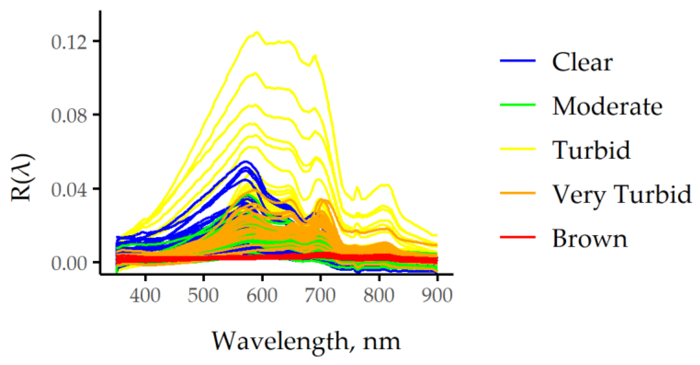
3.1. Description of OWT Classification

The OWT classification divided inland and coastal waters into five classes based on reflectance spectrum features. As shown in Figure 2, each OWT had a different R(λ) and was associated with a specific bio-optical condition. The R(λ) of the Clear OWT had a maximum at wavelengths between 540 and 580 nm, and the absorption influence from OSC was lowest in the blue part of the spectrum. This OWT corresponded to water with low OSC concentrations and the highest water transparency. As for the Clear OWT, the maximum R(λ) of the Moderate OWT occurred at wavelengths between 540 and 580 nm; however, the slope of R(λ) was sharper in the Moderate OWT due to the larger influence of OSC absorption. The OSC concentrations increased. In the Turbid OWT, the maximum R(λ) was in the green part of the spectrum, and the R(λ) values were the highest of all OWT types between approximately 500 and 700 nm. TSM was the dominant OSC in Turbid waters. In the Very Turbid OWT, the maximum R(λ) occurred between 685 and 715 nm; this was due to the strong Chl-a peak which was associated with phytoplankton blooms. Chl-a was the dominant OSC in Very Turbid waters. The R(λ) of the Brown OWT had very low values and reached the maximum in the red part of the spectrum. Waters appeared dark or reddish and dominated by CDOM.

The spectral scales of both MSI and OLCI preserved key features of the OWT classification. The R(λ) values of the OWTs were calculated using sensor-specific SRFs for the OLCI, MSI, MODIS, and OLI bands. OLCI has the most bands to follow hyperspectral results. Additionally, OLCI has four bands in the red part of the spectrum, where the Chl-a absorption peak is located. MSI was designed for the remote sensing of terrain and has a better spatial resolution; although it has fewer bands, it nevertheless captures differences in reflectance between the OWTs to a high degree. MODIS has a similar number of bands to MSI; however, the band central wavelengths (CWL) are different. Therefore, the reflectance spectra of the Turbid and Very Turbid OWTs are similar. In the Very Turbid OWT, a strong maximum R(λ) in the red part of the spectrum was no longer observed, with the maximum being shifted into the green part of the spectrum. The R(λ) of OWTs measured by OLI were the most similar to each other, with only the Brown OWT being strongly different; however, R(λ) features around 700 nm were lost since OLI has no band at this wavelength.

Classification Sensitivity

The sensitivity of the determination of OWTs was influenced differently by the OWT, sensor type, and spectral range. Figure 3 shows a detailed local sensitivity analysis of the OWT results. The Clear OWT was most sensitive to a decrease of local sensitivity factor 1 parameter (R(λ) values in the wavelength range of 400–500 nm). A decrease of factor 1 input values by more than 40% (i.e., changing the R(λ) values in the wavelength range of 400–500 nm by more than 40%) caused the OWT to change to Moderate. The Moderate OWT was sensitive to sensor type and wavelength range. A decrease of factor 1 and factor 2 (R(λ) values in the wavelength range of 500–700 nm) could cause the spectra to be classified as Turbid, Very Turbid, or Brown. Additionally, the Moderate OWT was sensitive to both increases and decreases in factor 3 (R(λ) values in the wavelength range of 700–900 nm). Regarding sensor type, for Ramses, a change of input parameter values of more than 60% was required to output a different OWT, while a change of just 20% was required for MSI. The Turbid OWT was the most sensitive to changes in factor 3. A decrease of factor 3 (e.g., 10% for MSI) changes the OWT to Moderate, while an increase of factor 3 changed the OWT into Very Turbid. Additionally, decreases of factor 1 or factor 2 of more than 30% shifted the classification to a Very Turbid or Brown OWT. The Very Turbid OWT was less sensitive to changes in the blue part of the spectrum and most sensitive to changes in the red part of the spectrum. Decreases in factor 3 changed the OWT to Turbid or Moderate. Increases in factor 2 caused spectra to be classified as Turbid, while decreases in factor 2 caused spectra to be classified as Brown. The Brown OWT was sensitive to increases of factor 2 and decreases of factor 3. Changes of factor 1 had a minimal impact on the classification of the Brown OWT.

An analysis treating satellite sensor bands as factors revealed that OLCI spectra were less sensitive to changes in input than MSI spectra. For OLCI spectra, the most sensitive OWT was Turbid when observed with bands 6 and 7, when a 30% change of input value would make an output OWT different. Usually, a change of input value of less than 70% did not change the classification assessment. MSI spectra were more sensitive to any input variation. This was especially true for MSI bands 3 and 5, where an input variation of more than 30% changed the designated OWT, except for the Clear and Moderate OWTs, where a variation of 70% and 20%, respectively, was required to affect the classification result.

3.2. Examples of Environmental Effects on the Variability of In Situ Measurements of R(λ)

As R(λ) depend on OSC concentrations, light conditions above the water surface, and water surface roughness [39], environmental effects were studied with a logistic regression model based on the variability in the in situ measured R(λ) and collected background information such as wind speed, wave height, cloudiness, and the presence of the direct sunlight. According to the model results, the wave height (p-value = 0.007), wind speed (p-value = 0.03), cloudiness (p-value = 0.0005) and partial covering of sun (p-value = 0.02) were important parameters that affected the probability of a rise in the measurement uncertainty of R(λ). The correct geometric positioning of radiometers during the measurements was essential. Additionally, however, increased wind speed or wave height affected ship stability, which led to unstable measurement conditions and therefore to an increase in measurement uncertainty. In the measurement stations affected by increased wind speed or wave height, the shape of the R(λ) spectrum remained the same; however, the R(λ) values varied strongly (by 17%–56%) in all spectral areas (

Table 1. Examples of variability of in situ measurements of R(λ) with different environmental factors and calibration uncertainty for selected wavelength ranges.

Source of Variability	No. of Spectra	Coefficient of Variation (%)
		400–500 nm	500–700 nm	700–900 nm
High wind speed (10 m·s−1)	11	45	19	51
High wave height (0.6 m)	76	35	17	56
Changing clouds (see Figure 4a)	92	108	84	859
Calm sea and clear sky	16	6.7	2.7	7.8
Instrument calibration		6.6	4.7	6.5

). When whitecaps started to appear on the water surface, the shape of the R(λ) spectrum changed at shorter wavelengths and R(λ) values increased. However, at times the wind speed was over 7 m·s⁻¹ but the water surface was calm and the variability of R(λ) was small (around 10%).

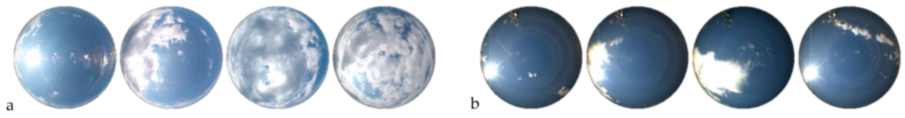
The second strong influence on the quality of R(λ) measurements was the presence of clouds. Generally, measurements made with a clear or overcast sky gave reliable results. However, when the cloud conditions started to change, the measured R(λ) usually started to vary, and data analysis was often difficult. Figure 4a shows a case when measurements started with an almost clear sky, yet for 19 minutes later the whole sky contained clouds while the sun remained visible. The measured R(λ) varied by 84% between 400–700 nm and by over 100% at shorter and longer wavelengths. A total of 13 of 92 spectra had negative values, and spectra with higher values of R(λ) were strongly dominated by the L_d(λ) spectra.

However, the all sky camera images revealed that the presence of clouds did not always ruin the measurements. For example, in the case shown in Figure 4b, clouds passed in front of the sun during the measurement but did not pass through the instrument’s field of view (which is located at the top of the pictures). The variability of the radiance and irradiance measurements around 500 nm were 15% and 17.7%, respectively, while the deviation of R(λ) stayed within 4.6%.

3.3. Classification of OWT from In Situ Measurements of R(λ)

The classification of OWT based on in situ measurements of R(λ) by Ramses at 180 stations are shown in Figure 5, and the range of the variation of the OSC concentrations and Secchi depth for OWTs are shown in

Table 2. The OWTs as determined from R(λ) and the corresponding Secchi depths and OSC concentrations based on the 180 measurements stations. Values are means with standard deviation given in parentheses.

OWT	No. of Stations	Secchi Depth, m	Chl-a 1	TSM 2	aCDOM(380) 3
Clear	39	3.3 (1.5)	6.0 (9.4)	4.4 (3.9)	1.19 (0.9)
Moderate	34	1.7 (0.6)	12.0 (8.6)	6.6 (4.5)	0.71 (0.5)
Turbid	76	0.9 (0.4)	19.4 (11.2)	13.4 (10.5)	1.23 (1.3)
Very Turbid	24	0.7 (0.2)	34.9 (14.0)	14.4 (4.1)	1.51 (0.4)
Brown	7	0.6 (0.2)	17.9 (7.6)	6.5 (4.6)	9.63 (4.2)

¹ Concentration of chlorophyll a, mg·m⁻³. ² Concentration of total suspended matter, mg·L⁻¹. ³ Absorption coefficient of colored dissolved organic matter at wavelength 380 nm, m⁻¹.

. The OWT for each measurement station was determined by the maximum likelihood calculated with Equation (3).

The Clear OWT was assigned to the R(λ) of 39 measurement stations. The maxima of R(λ) were between 540 and 580 nm, and a Chl-a peak was barely visible. This OWT corresponded to the most transparent waters (maximum Secchi depth of 6.5 m) and the lowest OSC concentrations. As shown in Table 2, the mean CDOM value of the Clear OWT was 1.19 m⁻¹. This value was higher than expected. More specifically, the mean CDOM value of the Clear OWT from the Wadden Sea was 1.9 m⁻¹, and the mean value was 0.4 m⁻¹ for the rest of the water bodies (different measurement techniques were used to determine CDOM values). Based on the OSC concentrations (Chl-a: 60 mg·m⁻³) and the low Secchi depth of 0.5 m, it is likely that one station was misclassified as the Clear OWT. At this station, measurement conditions (low sun elevation angle of 13°, wind speed of 5 m·s⁻¹, and the presence of waves and whitecaps) strongly affected reflectance spectra, with values being significantly increased in the blue part of the spectrum.

The Moderate OWT was assigned to the R(λ) of 34 measurement stations, with a maximum similarly to the Clear OWT between 540 and 580 nm and with a slightly steeper slope in the blue part of the spectrum. OSC concentrations were slightly higher than for the Clear OWT; however, no particular OSC dominated the others.

The Turbid OWT was the most frequent in our dataset, with the R(λ) of 76 stations being assigned to this OWT. The R(λ) of the Turbid OWT had the highest absolute values of all the OWTs; however, the maximum value of R(λ) varied greatly within this OWT. Waters classified as Turbid were strongly influenced by TSM, which had a maximum value of 62.4 mg·L⁻¹. At seven stations, the OSC concentration was too low (TSM under 4 mg·L⁻¹) and the Secchi depth was too high (over 1.6 m) to fit into the Turbid OWT; therefore, it is likely that these waters rather belonged to the Clear OWT. These measurements were made in low light conditions (in September or in early morning) or during strong wind, which affected the stability of the spectra.

The Very Turbid OWT was assigned to the R(λ) of 24 stations. These spectra had a maximum in the red part of the spectrum and showed clear Chl-a peak. These stations had high Chl-a values, with a mean value of 34.9 mg·m⁻³ and a maximum value of 71.8 mg·m⁻³.

The Brown OWT was the least frequent of all OWTs, being assigned to the R(λ) of seven stations. These stations had very low R(λ) values (under 0.005), having maxima in the red part of the spectrum and CDOM values at 380 nm of between 4.3 and 14.7 m⁻¹.

Classification of OWT Using In Situ Measurements of R(λ) Convoluted into Satellite Bands

The accuracy of OWT assignment was 95% for both the MSI and OLCI bands and 71% for the OLI bands. Confusion matrices between the OWTs assigned on in situ measurements of R(λ) (set as the true OWT value) and those which were assigned based on in situ measurements of R(λ) convoluted various sensor bands using sensor-specific SRFs (set as the predicted OWT value) were constructed to investigate the usefulness of different satellite data for OWT classification. As shown in Figure 6, the OLCI confusion matrix illustrates that a strong distinction was made between the Clear and Brown OWTs (100% correct assignment), while the lowest assignment accuracy (92%) was observed for the Very Turbid OWT, with 8% of spectra being misclassified as Turbid. The MSI confusion matrix demonstrates a strong distinction for the Clear, Very Turbid, and Brown OWTs (100% correct assignment); however, some Turbid spectra were misclassified as Very Turbid (7%) and Moderate (1%). The MODIS and OLI confusion matrices demonstrate significant misclassification for the Turbid and Very Turbid OWTs; in particular, using the OLI data, 55% of Turbid waters were misclassified.

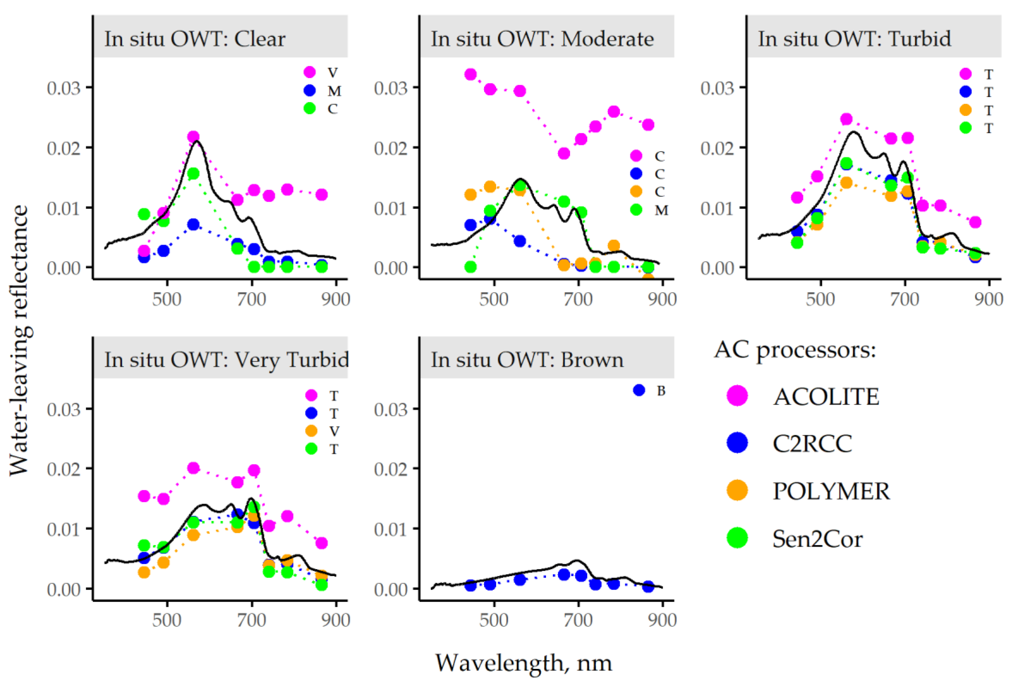
3.4. R(λ) and OWT Match-Ups Affected by Different Atmospheric Corrections (ACs)

For match-ups points away from the shore, MSI images processed with the C2RCC, POLYMER, and Sen2Cor AC processors gave quite similar values of R(λ), while MSI images processed with the ACOLITE AC processor commonly overestimated R(λ). However, C2RCC was not able to capture the maximum R(λ) in the red part of the spectrum. For small lakes, the situation was different, and AC processors did not provide any results in some cases. For example, only C2RCC data were derived for small lakes of the Brown OWT. For MSI images with 14 match-ups, all OWTs were captured (Table A1). Figure 7 shows a comparison between OWTs obtained using in situ measurements of R(λ) and OWTs obtained from MSI images processed with different ACs. OWTs obtained using the MSI-based R(λ) after processing with the POLYMER AC had the highest number of correct classifications (seven of eight). However, POLYMER was not able to reproduce R(λ) for six match-ups out of 14. In most cases, C2RCC and Sen2Cor were not able to correctly classify the Turbid OWT. Additionally, OWT classifications made using R(λ) derived from MSI images processed with the ACOLITE AC were correct in only one case.

Values of R(λ) derived from OLCI images processed with the AC processors ALTNNA and C2RCC were more accurate than those derived from OLCI images processed with the standard AC processor L2. A comparison of in situ measurements of R(λ) derived from OLCI images processed with different ACs showed that L2 strongly underestimated R(λ) at short wavelengths, sometimes even giving negative values. The R(λ) derived from OLCI images with C2RCC and ALTNNA were similar; however, ALTNNA overestimated R(λ) at shorter wavelengths and slightly underestimated R(λ) at other wavelengths. Figure 8 shows a comparison of OWTs determined based on the in situ measurements of hyperspectral R(λ) and OWTs determined using R(λ) derived from OLCI images processed with different ACs. In OLCI match-ups (Table A1), the Turbid, Moderate, and Very Turbid OWTs were most frequently estimated from in situ measurements of R(λ). Only one measurement station was classified as Clear, and none were classified as Brown. The OWTs determined using R(λ) derived from OLCI images processed with the C2RCC AC had the highest classification accuracy (16 of 34), with the Turbid OWT having an especially high accuracy (eight of 14). When using OLCI images processed with the ALTNNA AC, 15 of 34 OWTs were correctly classified, and the highest classification accuracy was obtained for Moderate OWTs. L2 had the lowest classification accuracy for OWTs. When C2RCC or ALTNNA misclassified an OWT, in most cases the Clear OWT was then assigned. If L2 misclassified an OWT, then the Very Turbid OWT was commonly assigned.

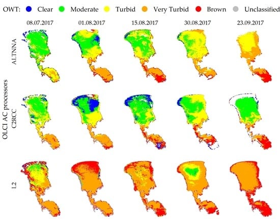
3.5. Spatial and Temporal Variability of OWTs Derived from Satellite Images Processed with Different ACs

The spatial and temporal variabilities of OWTs classified based on OLCI images processed with the ALTNNA and C2RCC AC processors were similar, while OWTs classified based on OLCI images processed with the L2 AC processor had different spatial and temporal variabilities. OWT classification was applied to OLCI images of Lake Peipsi acquired during July–September 2017 processed with the ALTNNA, C2RCC, and L2 AC processors. Lake Peipsi is large, shallow, optically complex, and very dynamic water body, and it has a strong north–south OSC concentration gradient. In mid-summer, the OSC concentrations in the northern part of Lake Peipsi were lower, and waters were mainly classified as the Moderate OWT when using images processed using the ALTNNA and C2RCC AC processors (Figure 9). At the same time, waters in the narrower southern part of Lake Peipsi were classified as Very Turbid. At the end of August, waters were widely classified as Turbid in the northern part of Lake Peipsi and as Brown in the southern part. In September (i.e., after the summer bloom), when OSC concentrations decreased, the OWT classified in the northern part of the lake returned to Moderate. OLCI images processed with the L2 AC processor were mainly classified as Very Turbid and Brown. In the southern part of Lake Peipsi, the OWT classification was similar to that obtained using the OLCI images processed with the C2RCC AC. However, when using the L2 AC, the Moderate and Turbid OWTs were usually misclassified in the northern part of Lake Peipsi. The ability of OLCI images processed with the L2 AC processor to correctly classify the Moderate and Turbid OWTs was affected by the shape of R(λ), as the first maximum around 550 nm was very weak.

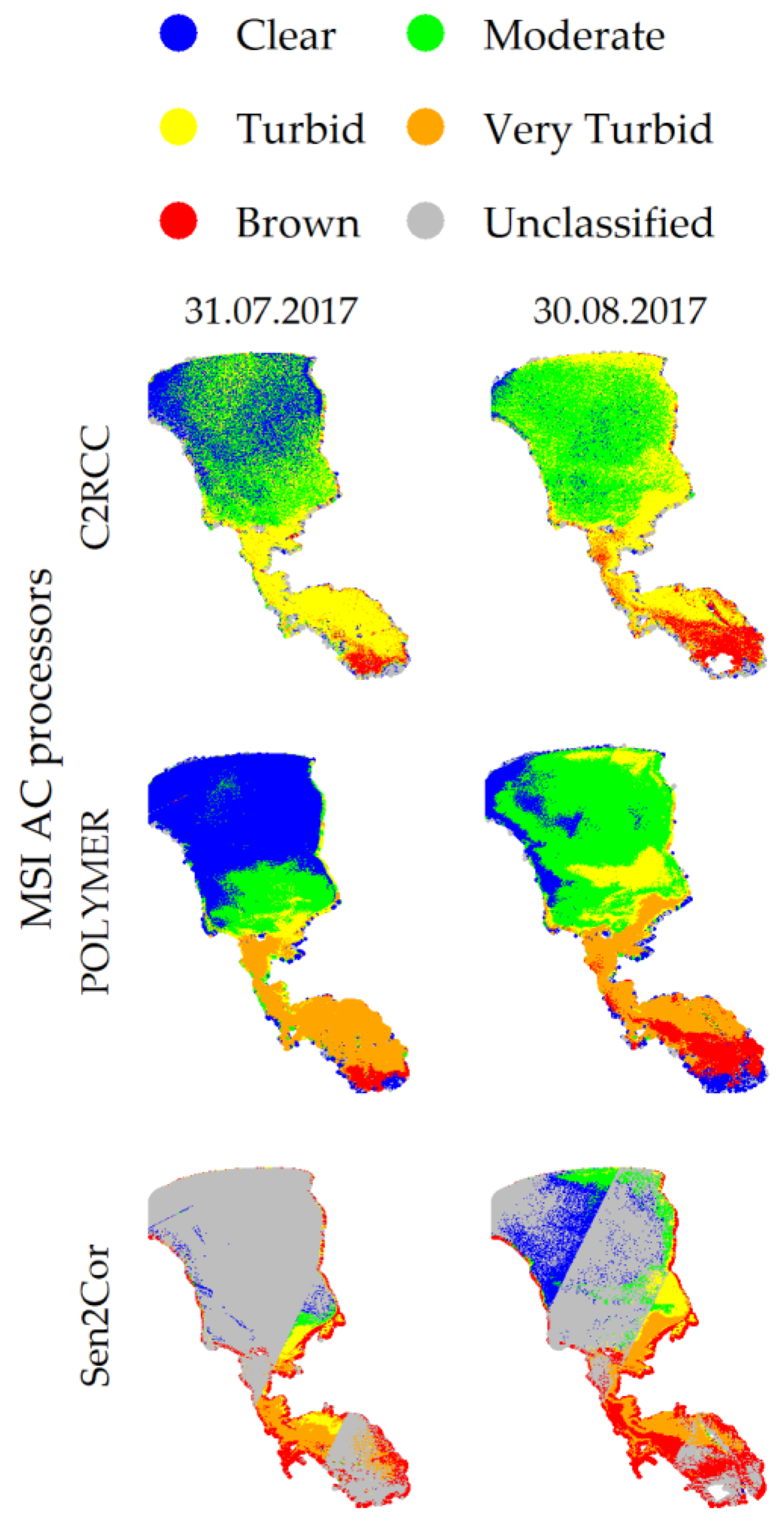
The same approach was applied to MSI images processed with the C2RCC, POLYMER, and Sen2Cor AC processors. The spatial and temporal variabilities of OWTs were determined. As shown in Figure 10, MSI images processed with the C2RCC and POLYMER AC processors gave similar results. Before the summer blooming of phytoplankton in the northern part of Lake Peipsi, MSI images processed with POLYMER were mainly classified as the Clear OWT, while MSI images processed with C2RCC were mainly classified as Clear and Moderate. In the southern part of Lake Peipsi, the dynamics of the Brown OWT were similar for all AC processors; however, differences were found in the classification of Turbid and Very Turbid OWTs. In August, OSC concentrations were higher, and OWTs with higher OSC concentrations were classified.

4. Discussion

By examining the key features of R(λ) spectra, it was possible to classify waters into different OWTs dominated by Chl-a, TSM, or CDOM. These OWTs are complex indices that can be used to evaluate the health of a waterbody. Since OWTs take multiple parameters into account, they can be more valuable than maps with one parameter (e.g., TSM, Chl-a, CDOM, and Secchi) to capture changes and to understand the reason for changes. Additionally, the use of OWTs helps to develop algorithms for optically complex waters to derive OSC concentrations and helps to choose a working AC processor for a region of interest.

For in situ measurements of R(λ), it is necessary to remember that the estimated R(λ) are affected by the amount of OSC in the water, as well as by the light conditions above the water surface, the air-water interface, and measurement geometry [39]. For example, measurements made with a low sun elevation angle (performed early in the morning, late in the evening, or in autumn) often led to the misclassification of OWTs. R(λ) values were lower and OWTs were classified differently compared to measurements of water with the same OSC concentration made at mid-day in summer. Additionally, the system of three sensors which was used to derive R(λ) was based on strict geometrical rules and was sensitive to the effects such as high wind, waves, whitecaps, foam, clouds, and sun glint. Additionally, in situ R(λ) measurements were difficult to perform well in CDOM-rich waters. Often, in situ R(λ) strongly overestimated the spectra in the blue region, which led to the misclassification of OWTs (Table A1; rows 4,5). In some Brown OWT cases, the shape of the R(λ) spectra derived from the satellite were similar, strongly overestimating the blue region; however, this could have been caused by an adjacency effect since these were measurements stations from small lakes. These Brown OWT cases need to be studied in more detail in the future.

Sensitivity analyses showed, as expected, that the OWT classification was sensitive to changes in the input R(λ). When sun glint led to an increase of the R(λ) values in the blue part of the spectrum [40], waters of the Moderate OWT could be classified as the Clear OWT. Furthermore, when R(λ) values in the red part of the spectrum increased due to incorrect measurement geometry or the presence of clouds [41], then waters of the Moderate OWT could be classified as Turbid or Very Turbid. The changes in the hyperspectral R(λ) input must be bigger than 40% to affect the OWT classification result, except for the Very Turbid OWT, for which a decrease in the R(λ) value in the red part of the spectrum of over 20% led to a change of OWT assignment. As shown in Table 1, the variability in the in situ measurements of R(λ) could be more than 40% for certain wavelength ranges.

In the context of satellite application, this study showed that MSI and OLCI images can be used for OWT classification. However, as shown in Figure 9 and Figure 10, the choice of AC processor strongly affected the OWT classification, although similar water-body spatial and temporal dynamics were obtained for all of the AC processors analyzed in this study. We focused on how different AC processors were able to retrieve different OWTs. Based on the available R(λ) match-ups, we suggest using the C2RCC AC processor on the MSI and OLCI images of the boreal region investigated in this study. The processing of OLCI images with the L2 AC processor led to a strong underestimation of R(λ), even leading to negative values at shorter wavelengths. However, compared to other AC processors, for waters classified as the Very Turbid OWT, the L2 AC processor better captured the maximum in the red part of the spectrum. The ALTNNA AC processor performed similarly to C2RCC; however, slightly higher values of R(λ) were usually obtained. Additionally, for waters with higher OSC concentrations, the first maximum at 550–580 nm had lower values. As shown in Figure 9, the variation in OWT obtained with the C2RCC AC processor was similar to that obtained by Reinart and Valdmets [42], who performed OWT classification based on OSC concentrations. OLCI images processed with the L2 AC processor mainly gave OWT classifications of the Very Turbid and Brown types. Since the first maximum of R(λ) at 550–580 nm was strongly underestimated when the L2 processor was used while the maximum in the red part of the spectrum was well captured, the resulting spectral shape of R(λ) was distorted. Moreover, sensitivity analyses confirmed that a decrease of the R(λ) values at 500–700 nm caused Moderate and Turbid OWTs to be assigned as Very Turbid or Brown.

The presented OWT classification was applied to OLCI images acquired in the Baltic region (Figure 11). The results showed that the areas of the Baltic Sea with low OSC concentrations were classified as Clear, while coastal areas where river inflows were present were classified as different OWTs. Waters of the Gulf of Finland were mainly classified as Clear; however, further east, where the Neva River inflows, waters were widely classified as Turbid. In the Gulf of Riga, where water exchange is weaker and affected by the Pärnu and Daugava rivers, the OWT varied from Brown to Clear. Using the OWT classification performed in this study, it is possible to follow the movements of river water masses. Additionally, the OWT classification for larger lakes showed a reasonable correspondence with the results of previous studies [42,43,44,45]. Some small lakes and pixels affected by the adjacency effect were often classified as Clear.

Finally, we tested our approach on Río de la Plata (the La Plata River; South America) to investigate its applicability to a different region. Río de la Plata is a shallow and highly turbid estuary located between Argentina and Uruguay. Its most important tributaries are the Paraná River, the Paraguay River, and the Uruguay River, and it discharges into the Atlantic Ocean. As shown in Figure 12, the highly turbid waters of the upper and middle estuary were classified as Turbid, the waters of the outer estuary were mainly classified as Moderate, and the waters of the Atlantic Ocean were classified as Clear. The OWT classification agrees well with literature values of TSM (mean values of 100–300 mg·L⁻¹ [46]) and Chl-a (values from 1 to 30 mg·m⁻³ [47]). Additionally, the calculated OWT spatial and temporal dynamics agree well with the winter and summer seasons when water masses move differently [47].

5. Conclusions

The availability of free data from the MSI and OLCI sensors with high spectral, spatial, and temporal resolution has generated wide interest in the use of remote sensing to monitor water quality in inland and coastal waters. Such waters are optically complex and are independently influenced by Chl-a, TSM, and CDOM. OWT classification is a way to monitor the optical diversity of aquatic systems. In this study, we developed a simple new OWT classification system which takes R(λ) as input and uses key spectral features to divide water into five OWTs. Each OWT has different reflectance spectra which reflect different bio-optical conditions. We focused our research on northern boreal lakes and coastal areas without extreme optical conditions such as very transparent or extremely turbid waters. We additionally showed that this OWT classification approach is applicable to another region.

We demonstrated that two sensors with different SRFs—the OLCI, onboard the Sentinel-3 satellite, which is designed for the remote sensing of water, and the MSI, onboard the Sentinel-2 satellite, which is designed for the remote sensing of land—can distinguish all five OWTs. Therefore, the approach proposed in this study has the ability to monitor changes of OWTs in more water bodies, in addition to coastal waters and lakes, using MSI images. We also analyzed the sensitivity of OWT classification related to the uncertainty of R(λ) and to the variety of AC processors. Therefore, it is necessary to select an appropriate AC for the region of interest. In this study, the C2RCC AC processor was found to be the most accurate and reliable for use with MSI and OLCI images. The simple approach proposed in this study can provide a basis for understanding the seasonal and spatial variabilities of water bodies and for planning lake-monitoring programs. Additionally, since each OWT describes different bio-optical conditions, this study provides a good foundation to develop algorithms to derive OSC concentrations using OWTs.

References

1. Morel, A.; Prieur, L. Analysis of variations in ocean color. Limnol. Oceanogr. 1977, 22, 709–722. [Google Scholar] [CrossRef]
2. Jerlov, N.G. Classification of sea water in terms of quanta irradiance. ICES J. Mar. Sci. 1977, 37, 281–287. [Google Scholar] [CrossRef]
3. Reinart, A.; Herlevi, A.; Arst, H.; Sipelgas, L. Preliminary optical classification of lakes and coastal waters in Estonia and south Finland. J. Sea Res. 2003, 49, 357–366. [Google Scholar] [CrossRef]
4. McKee, D.; Cunningham, A.; Dudek, A. Optical water type discrimination and tuning remote sensing band-ratio algorithms: Application to retrieval of chlorophyll and Kd(490) in the Irish and Celtic Seas. Estuar. Coast. Shelf Sci. 2007, 73, 827–834. [Google Scholar] [CrossRef]
5. Naumann, E. The Scope and Chief Problems of Regional Limnology. Int. Rev. Hydrobiol. 1929, 21, 423. [Google Scholar] [CrossRef]
6. Wernand, M.R.; Hommersom, A.; van der Woerd, H.J. MERIS-based ocean colour classification with the discreteForel–Ule scale. Ocean Sci. 2013, 9, 477–487. [Google Scholar] [CrossRef]
7. The European Parliament; The Council of the European Union. Directive 2000/60/EC of the European Parliament and of the Council of 23 October 2000 establishing a framework for Community action in the field of water policy. Off. J. Eur. Communities 2000, 43, 275–346. [Google Scholar]
8. Eleveld, M.A.; Ruescas, A.B.; Hommersom, A.; Moore, T.S.; Peters, S.W.M.; Brockmann, C. An Optical Classification Tool for Global LakeWaters. Remote Sens. 2017, 9, 420. [Google Scholar] [CrossRef]
9. Spyrakos, E.; O’donnell, R.; Hunter, P.D.; Miller, C.; Scott, M.; Simis, S.G.H.; Neil, C.; Barbosa, C.C.F.; Binding, C.E.; Bradt, S.; et al. Optical types of inland and coastal waters. Limnol. Oceanogr. 2018, 63, 846–870. [Google Scholar] [CrossRef]
10. Vantrepotte, V.; Loisel, H.; Dessailly, D.; Mériaux, X. Optical classification of contrasted coastal waters. Remote Sens. Environ. 2012, 123, 306–323. [Google Scholar] [CrossRef]
11. Shi, K.; Li, Y.; Li, L.; Lu, H.; Song, K.; Liu, Z.; Xu, Y.; Li, Z. Remote chlorophyll-a estimates for inland waters based on a cluster-based classification. Sci. Total Environ. 2013, 444, 1–15. [Google Scholar] [CrossRef] [PubMed]
12. Traykovski, L.V.M.; Sosik, H.M. Feature-based classification of optical water types in the Northwest Atlantic based on satellite ocean color data. J. Geophys. Res. 2003, 108, 3150. [Google Scholar] [CrossRef]
13. Jackson, T.; Sathyendranath, S.; Mélin, F. An improved optical classification scheme for the Ocean Colour Essential Climate Variable and its applications. Remote Sens. Environ. 2017, 203, 152–161. [Google Scholar] [CrossRef]
14. Moore, T.S.; Campbell, J.W.; Dowell, M.D. A class-based approach to characterizing and mapping the uncertainty of the MODIS ocean chlorophyll product. Remote Sens. Environ. 2009, 113, 2424–2430. [Google Scholar] [CrossRef]
15. Shen, Q.; Li, J.; Zhang, F.; Sun, X.; Li, J.; Li, W.; Zhang, B. Classification of Several Optically Complex Waters in China Using in Situ Remote Sensing Reflectance. Remote Sens. 2015, 7, 14731–14756. [Google Scholar] [CrossRef] [Green Version]
16. Gordon, H.R.; Brown, O.B.; Evans, R.H.; Brown, J.W.; Smith, R.C.; Baker, K.S.; Clark, D.K. A semianalytic radiance model of ocean color. J. Geophys. Res. 1988, 93, 10909–10924. [Google Scholar] [CrossRef]
17. Hommersom, A.; Peters, S.; Wernand, M.R.; de Boer, J. Spatial and temporal variability in bio-optical properties of the Wadden Sea. Estuar. Coast. Shelf Sci. 2009, 83, 360–370. [Google Scholar] [CrossRef]
18. TO Water Remote Sensing Database. Available online: https://water.to.ee/ (accessed on 25 July 2019).
19. Institute of Zoology and Botany at the Estonian Agricultural University. Organic matter, colour and Transparency of water. In Lake Peipsi: Meteorology, Hydrology, Hydrochemistry; Nõges, T., Ed.; Sulemees Publishers: Tartu, Estonia, 2001; pp. 117–121. [Google Scholar]
20. Reinart, A.; Herlevi, A. Diffuse attenuation coefficient in some Estonian and Finnish lakes. Proc. Est. Acad. Sci. Biol. Ecol. 1999, 48, 267–283. [Google Scholar]
21. Tilstone, G.H.; Moore, G.F.; Doerffer, R.; Røttgers, R.; Ruddick, K.G.; Pasterkamp, R.; Jørgensen, P.V. Regional Validation of MERIS Chlorophyll products in North Sea REVAMP Protocols Regional Validation of MERIS Chlorophyll products. In Proceedings of the Working Meeting on MERIS and AATSR Calibration and Geophysical Validation (ENVISAT MAVT-2003), Frascati, Italy, 20–24 October 2003. [Google Scholar]
22. Vabson, V.; Kuusk, J.; Ansko, I.; Vendt, R.; Alikas, K.; Ruddick, K.; Ansper, A.; Bresciani, M.; Burmester, H.; Costa, M.; et al. Laboratory Intercomparison of Radiometers Used for Satellite Validation in the 400–900 nm Range. Remote Sens. 2019, 11, 1101. [Google Scholar] [CrossRef]
23. MSI SRFs. Available online: https://earth.esa.int/web/sentinel/user-guides/sentinel-2-msi/document-library/-/asset_publisher/Wk0TKajiISaR/content/sentinel-2a-spectral-responses (accessed on 24 July 2019).
24. OLCI SRFs. Available online: https://sentinel.esa.int/web/sentinel/technical-guides/sentinel-3-olci/olci-instrument/spectral-response-function-data (accessed on 24 July 2019).
25. MODIS SRFs. Available online: https://mcst.gsfc.nasa.gov/calibration/parameters (accessed on 24 July 2019).
26. OLI SRFs. Available online: https://landsat.gsfc.nasa.gov/preliminary-spectral-response-of-the-operational-land-imager-in-band-band-average-relative-spectral-response/ (accessed on 24 July 2019).
27. European Commission; Joint Research Centre (European Commission). Manual for Monitoring European Lakes Using Remote Sensing Techniques; Lindell, T., Pierson, D., Premazzi, G., Zilioli, E., Eds.; Office for Official Publications of the European Communities: Luxembourg, 1999; pp. 29–69. [Google Scholar]
28. Jeffrey, S.W.; Humphrey, G.F. New spectrophotometric equations for determining chlorophylls a, b, c1 and c2 in higher plants, algae and natural phytoplankton. Biochem. Physiol. Pflanz. 1975, 167, 191–194. [Google Scholar] [CrossRef]
29. Copernicus Open Access Hub. Available online: https://scihub.copernicus.eu/ (accessed on 25 July 2019).
30. ACOLITE: Atmospheric Correction for Aquatic Applications of Landsat and Sentinel-2. Available online: https://github.com/acolite/acolite (accessed on 25 July 2019).
31. C2RCC—Water Quality from Space with the SNAP C2RCC Processor. Available online: https://www.brockmann-consult.de/c2rcc-water-quality-from-space-with-the-snap-c2rcc-processor/ (accessed on 25 July 2019).
32. HYGEOS—Polymer. Available online: https://www.hygeos.com/polymer (accessed on 25 July 2019).
33. Sen2Cor|STEP. Available online: https://step.esa.int/main/third-party-plugins-2/sen2cor/ (accessed on 25 July 2019).
34. SNAP|STEP. Available online: https://step.esa.int/main/toolboxes/snap/ (accessed on 25 July 2019).
35. Copernicus Online Data Access. Available online: https://coda.eumetsat.int/ (accessed on 25 July 2019).
36. Ansper, A.; Alikas, K. Retrieval of Chlorophyll a from Sentinel-2 MSI Data for the European Union Water Framework Directive Reporting Purposes. Remote Sens. 2019, 11, 64. [Google Scholar] [CrossRef]
37. Homayouni, S.; Roux, M. Hyperspectral image analysis for material mapping using spectral matching. Int. Arch. Photogramm. Remote Sens. Spat. Inf. Sci. 2004, 35, 49–54. [Google Scholar]
38. Morio, J. Global and local sensitivity analysis methods for a physical system. Eur. J. Phys. 2011, 32, 1577–1583. [Google Scholar] [CrossRef]
39. Mobley, C.D. Light and Water: Radiative Transfer in Natural Waters; Academic Press: San Diego, CA, USA, 1994; pp. 67–77. [Google Scholar]
40. Kutser, T.; Vahtmäe, E.; Paavel, B.; Kauer, T. Removing glint effects from field radiometry data measured in optically complex coastal and inland waters. Remote Sens. Environ. 2013, 133, 85–89. [Google Scholar] [CrossRef]
41. Ruddick, K.G.; De Cauwer, V.; Park, Y.J.; Moore, G. Seaborne measurements of near infrared water-leaving reflectance: The similarity spectrum for turbid waters. Limnol. Oceanogr. 2006, 51, 1167–1179. [Google Scholar] [CrossRef] [Green Version]
42. Reinart, A.; Valdmets, K. Variability of optical water types in Lake Peipsi. Proc. Est. Acad. Sci. Biol. Ecol. 2007, 56, 33–46. [Google Scholar]
43. Paavel, B.; Arst, H.; Reinart, A. Variability of bio-optical parameters in two North-European large lakes. Hydrobiologia 2008, 599, 201–211. [Google Scholar] [CrossRef]
44. Piirsoo, K.; Laas, A.; Meinson, P.; Nõges, P.; Pall, P.; Viik, M.; Vilbaste, S.; Nõges, T. Changes in particulate organic matter passing through a large shallow lowland lake. Proc. Est. Acad. Sci. 2018, 67, 93–105. [Google Scholar] [CrossRef]
45. Soomets, T.; Uudeberg, K.; Jakovels, D.; Kutser, T.; Brauns, A. The validation and comparison of the water quality products in Baltic lakes using Sentinel-2 and Sentinel-3 data. In Proceedings of the Living Planet Symposium. [CrossRef]
46. Knaeps, E.; Doxaran, D.; Dogliotti, A.; Nechad, B.; Ruddick, K.; Raymaekers, D.; Sterckx, S. The SeaSWIR dataset. Earth Syst. Sci. Data 2018, 10, 1439–1449. [Google Scholar] [CrossRef] [Green Version]
47. Huret, M.; Dadou, I.; Dumas, F.; Lazure, P.; Garçon, V. Coupling physical and biogeochemical processes in the Rio de la Plata plume. Cont. Shelf Res. 2005, 25, 629–653. [Google Scholar] [CrossRef]
Figure 1. The system of three TriOS-RAMSES hyperspectral radiometers used for the R(λ) measurements.
Remotesensing 11 02297 g001
Figure 2. R(λ) for each OWT (top) and R(λ) by OLCI, MSI, MODIS, and OLI bands calculated with sensor-specific SRFs (bottom).
Remotesensing 11 02297 g002
Figure 3. Local sensitivity analysis for OWT classification for sensors with different spectral scales. First row: Ramses with 1 nm step resolution; second row: OLCI; third row: MSI. Column 1: local sensitivity factor 1 (400–500 nm); column 2: factor 2 (500–700 nm); and column 3: factor 3 (700–900 nm). The original OWTs are indicated by different colors (determined at parameter deviation of 0%), and the sensitivity analysis of OWTs output is denoted as transitions between the OWTs. Input parameters vary from −90% to +100% on the x-axes.
Remotesensing 11 02297 g003
Figure 4. Changing cloud condition during the R(λ) measurements captured by all sky camera in stations with (a) big and (b) small variability of R(λ). Four images cover a time gap of approximately 20 minutes.
Remotesensing 11 02297 g004
Figure 5. In situ measured R(λ) classified into various OWTs by maximum likelihood calculated by Equation (3).
Remotesensing 11 02297 g005
Figure 6. Normalized confusion matrices showing the accuracy of OWT assignment using in situ measurements of R(λ) convoluted into the OLCI, MSI, MODIS, and OLI bands. Rows show the true OWTs determined from in situ measurements of R(λ) using Ramses, and columns show the predicted OWTs determined from the convoluted R(λ). The diagonal elements represent the situation where the predicted OWT is the same as the true OWT (i.e., correct classification).
Remotesensing 11 02297 g006
Figure 7. Examples of OWT determined using in situ measurements of R(λ) (black line) and OWT estimated from MSI images processed with different AC processors, namely ACOLITE, C2RCC, POLYMER, and Sen2Cor.
Remotesensing 11 02297 g007
Figure 8. Examples of OWTs determined from in situ measurements of R(λ) (black line) and OWTs determined from OLCI images processed with different AC processors, namely ALTNNA, C2RCC, and L2.
Remotesensing 11 02297 g008
Figure 9. Examples of OWTs obtained from OLCI images of Lake Peipsi acquired in July–September 2017 processed with the ALTNNA, C2RCC, and L2 AC processors.
Remotesensing 11 02297 g009
Figure 10. Examples of OWTs determined using MSI images of Lake Peipsi acquired during July and August 2017 processed with the C2RCC, POLYMER, and Sen2Cor AC processors.
Remotesensing 11 02297 g010
Figure 11. Classification of the OWT based on OLCI images of Estonian waters acquired on 02 May 2017 processed with the C2RCC AC processor.
Remotesensing 11 02297 g011
Figure 12. Estimation of R(λ) and classification of OWTs from OLCI images of Río de la Plata (the La Plata River; South America) acquired on 01 May 2017 processed with the C2RCC AC processor.
Remotesensing 11 02297 g012