On the Analysis of the Phase Unwrapping Process in a D-InSAR Stack with Special Focus on the Estimation of a Motion Model

Abstract

This paper analyses the critical phase unwrapping step in a differential interferometric phase (D-InSAR) stack where both the solving of conventional methods and alternative approaches are discussed. It can be shown that including the temporal relationship between interferograms in the phase unwrapping step improves the results. This leads to the three-dimensional extended minimum cost flow algorithm. To unwrap the phase in a multitemporal way a motion model has to be considered. The estimation of these parameters is an important step. By default, the parameters are estimated in an iterative search process, where in each step, a linear program has to be solved. The best parameters are defined by the minimal costs. Often the choice of this search space is not straightforward. Furthermore, with this discrete optimization function, the solution is often not unique. This paper presents an alternative way to estimate the motion model parameters by maximizing a continuous function, the ensemble phase coherence. With the help of a closed-loop simulation and real data, both methods, the standard and the alternative way, are numerically compared and analyzed. Consequently, it is shown that maximizing the ensemble phase coherence is a good alternative to the established iterative procedure. It offers the advantage that the run time can be reduced considerably and is thus well suited in the processing of large data sets.

1. Introduction

The differential interferometric phase (D-InSAR) contains information about relative topography changes between two acquisition times. Analyzing repeated orbits allows the generation of deformation time series. Therefore, data from several years are used and evaluated together in a so-called D-InSAR stack. There are two widely used methods to process these data altogether in a multitemporal way, the permanent scatterer interferometry [1] and the small baseline subset (SBAS) method [2].

The former one only uses stable pixels that show consistent backscattering characteristics over the entire stack. These stable pixels are called persistent scatterers. They are very rare and mostly occur in urban areas.

To achieve a denser spatial sampling, the SBAS method is preferred. This method only generates interferograms between SAR images with a small temporal and spatial baseline. By limiting the baselines, independent subsets can arise which are linked with the help of the Singular Value Decomposition method. The small baselines, together with multilooked data, reduce the decorrelation effects and the phase noise level. Consequently, the spatial sampling rate can be increased compared to the PSI method [2]. More recent algorithms combine stable and distributed scatterers to further increase the resolution, e.g., SqueeSAR [3].

In this paper, the differential interferometric data should be used to detect the ground deformation in the Lower-Rhine-Embayment in the southwest of North Rhine-Westphalia, Germany. The Lower-Rhine-Embayment is characterized by a very rural area with many forests in the south. Within this area, there is one of the largest brown coal occurrences in Europe represented by the still active open-cast mines Garzweiler, Hambach and Inden leading the surrounding Earth’s surface to subside [4]. Moreover, there are the closed coal mining regions Aachen and Erkelenz. The consequent rise of the groundwater level in the pits results in an elevation of the Earth’s surface. Regular monitoring measurements of these ground movements are therefore necessary. To detect them at a large-scale, the SBAS method should be used as stable scatterers are very rare in this region.

In a typical SBAS processing, the phase unwrapping is done iteratively to reduce phase unwrapping errors. However, the phase unwrapping remains a critical task in the analysis [5]. This paper will address the problem of unwrapping the observed interferometric phase.

1.1. The Phase Unwrapping Problem-State of the Art

The interferometric phase ${\psi }_{x_j}^{∆t_{\alpha \beta }}$ of two SAR images at times $t_{\alpha }$ and $t_{\beta }$ at pixel $x_j$ can only be measured modulo $2\pi$. This ambiguous phase is called the wrapped phase. Consequently, if the surface displacement is greater than a quarter of the radar wavelength (equal to $1.42$ cm for the ERS 1/2 satellites) or other effects, like topographic errors, atmosphere or noise occur, the interferogram cannot be uniquely inverted. To derive the information of interest, for instance, the deformation, the phase ambiguities have to be solved. Therefore, the absolute, so-called unwrapped phase

$$\begin{array}{c}\hfill {\varphi }_{x_j}^{∆t_{\alpha \beta }}={\psi }_{x_j}^{∆t_{\alpha \beta }}+2\pi k_{x_j}^{∆t_{\alpha \beta }}\forall x_j\in \mathcal{M}\end{array}$$

(1)

has to be obtained by adding an integer multiple $k_{x_j}^{∆t_{\alpha \beta }}$ of $2\pi$ to the wrapped phase. This has to be done for each pixel of the set $\mathcal{M}$ of pixels in the interferogram. As the phase unwrapping represents a large field of research, numerous algorithms exist, e.g., [6,7,8,9,10,11]. Basically, all of them start with the measured wrapped D-InSAR phases and consider the unwrapped phase as a continuous curve and thus as an integral of the phase gradients [12]. The wrapped measured phase gradients between two adjacent pixels $x_k$ and $x_l$ results in

$$\begin{array}{c}\hfill {\psi }_{∆x_{kl}}^{∆t_{\alpha \beta }}={\langle {\psi }_{x_l}^{∆t_{\alpha \beta }}-{\psi }_{x_k}^{∆t_{\alpha \beta }}\rangle }_{-\pi ,\pi }\forall ∆x_{kl}\in \mathcal{N},\end{array}$$

(2)

with the modulo-operator ${\langle .\rangle }_{-\pi ,\pi }$ and the set $\mathcal{N}$ of phase gradients in the interferogram. Assuming that the phase is sampled often enough and the unwrapped phase will not change by as much as half a cycle between adjacent pixels, the unwrapped phase ${\varphi }_{x_j}^{∆t_{\alpha \beta }}$ at pixel $x_j$ can be easily reconstructed up to an additive constant by integrating the wrapped phase gradients along any set ${\mathcal{N}}_{x_j}$ of phase gradients that connect a reference point $x_0$ and the pixel $x_j$

$$\begin{array}{c}\hfill {\varphi }_{x_j}^{∆t_{\alpha \beta }}={\displaystyle \sum _{\forall ∆x_{kl}\in {\mathcal{N}}_{x_j}}}{\psi }_{∆x_{kl}}^{∆t_{\alpha \beta }}+{\varphi }_{x_0}^{∆t_{\alpha \beta }}.\end{array}$$

(3)

The integral is replaced by a sum due to the discrete representation. The solution is path-independent and does not depend on the set ${\mathcal{N}}_{x_j}$ of phase gradients.

In reality, phase noise, atmospheric effects, sub-sampling or topographic effects lead to inconsistencies, meaning that the oriented sum of the phase gradients in one loop is unequal to zero in some cases, referred to as residue. The task is to correct for or to avoid these inconsistencies.

On the one hand, there are path-following methods, which unwrap each pixel locally starting from a reference point. One of the first and classic algorithms is Goldstein’s algorithm [13]. The so-called branch cuts are defined by connecting residues with an opposite sign so that the cut is neutralized. The phases can then be unwrapped in a consistent way if the branch cuts are not crossed. The algorithm works well for images with high coherence and moderate residue density [14]. However, areas which are trapped by branch cuts are inaccessible for the algorithm, resulting in spatially incomplete solutions.

On the other hand, there are global methods that find a global solution by minimizing a certain measure of misfit between the wrapped gradient data and the unwrapped solution. The two main global techniques are the minimum-norm method [15] and the minimum cost flow (MCF) approach [16]. The former one formulates the unwrapping process as the minimization problem

$$\begin{array}{c}\hfill {\displaystyle \sum _{\forall ∆x_{kl}\in \mathcal{N}}}{|{\varphi }_{∆x_{kl}}^{∆t_{\alpha \beta }}-{\psi }_{∆x_{kl}}^{∆t_{\alpha \beta }}|}^p\dots \min \end{array}$$

(4)

for the set $\mathcal{N}$ of phase gradients under the L${}_p$-norm. A typical algorithm is the least-squares method for $p=2$. The major difference to the local methods is that any value may be added to the measurements to ensure a continuity in the solution. It has the advantage that the phase could be unwrapped everywhere in the image. However, the solution will underestimate the phase slope as shown in [14].

The second main global technique is the MCF algorithm, first described in [16] to unwrap regularly sampled pixel in one interferogram. An adapted algorithm for solving sparse networks using a Delaunay triangulation of a set of pixels was introduced by [17]. The MCF approach deals with the assumption that the wrapped phase gradients differ from the unwrapped ones by an unknown multiple of $2\pi$

$${\varphi }_{∆x_{kl}}^{∆t_{\alpha \beta }}={\psi }_{∆x_{kl}}^{∆t_{\alpha \beta }}+2\pi k_{∆x_{kl}}^{∆t_{\alpha \beta }}$$

(5)

with the phase ambiguity factor of the phase gradient $k_{∆x_{kl}}^{∆t_{\alpha \beta }}$. The phase unwrapping is seen as the weighted L₁-norm minimization problem of the deviation between the estimated and unknown phase gradients of the unwrapped phases under the above assumption that both differ by an integer multiple of $2\pi$. This assumption prevents the errors from spreading effects [16]. Considering the structure, the problem could be transformed into a network, searching for the minimum cost flow, defined by the unknown phase ambiguity factor.

The MCF approach by [17] is a rather popular phase unwrapping operation based on the spatial, two-dimensional information of one interferogram. With respect to a multitemporal D-InSAR stack, there are several interferograms. Including the temporal relationship between the interferograms as additional information leads to an improvement in the accuracy of the solution in a similar way to which two-dimensional unwrapping provides an improvement over one-dimensional methods [18]. Three-dimensional phase unwrapping, where the temporal relationship between the interferograms represents the third dimension, could be achieved either using multiple steps or by an one-step algorithm. The relevant literature relating to three-dimensional phase unwrapping can be found in [5,18,19,20]. The second one extends the minimum-norm method according to [15] by the third dimension and describes a stepwise algorithm. [19,20] are based on the MCF approach. However, they consider the edge relationships rather than the triangle relationships, which result in closed loops. This leads to the parametric approach described in Section 2.2, which leads to a higher complexity.

This work focuses on the extended MCF (EMCF) algorithm [5] which is fully compatible to the SBAS method and can be very efficiently be solved as two simpler two-dimensional minimum cost flow problems. Both approaches, the two-dimensional MCF, and the three-dimensional EMCF, are compared and, in particular, the EMCF approach is further analyzed. The inclusion of the temporal relationship between the interferograms requires the consideration of a motion model. One important step is the estimation of the motion model parameters. The algorithm includes an iterative search process to estimate the parameters. This paper will present an alternative way that is numerically analyzed and tested using simulated and real data.

1.2. Outline

The structure of this paper is as follows. Section 2 deals with the two-dimensional MCF approach, where linear program solvers and network flow problems are addressed in this context. Afterwards, Section 3 describes the three-dimensional EMCF approach. Section 4 shows an analysis, where both approaches, MCF and EMCF, are applied to a simulated D-InSAR stack. In the analysis advantages and the disadvantages of the EMCF approach are discussed and ideas for improvement are analyzed and tested with simulated and real data in Section 5. A further discussion follows in Section 6 and the paper finishes with a conclusion.

2. Phase Unwrapping in 2D Using the MCF Approach

The MCF algorithm by [17] is a branch cut based algorithm to solve the phase unwrapping problem for one interferogram. The algorithm only uses so-called coherent pixels to reduce the noise. These are pixels with a stable backscattering characteristic, identified by the coherence values. Based on the set $\mathcal{M}$ with m coherent pixels a Delaunay triangulation in the azimuth/range plane with the set $\mathcal{N}$ of n spatial arcs and the set $\mathcal{R}$ of r defined triangles is computed. Figure 1 shows a small example consisting of $m=4$ pixels, $n=5$ arcs and $r=2$ triangles. Along each arc the wrapped phase gradient ${\psi }_{∆x_{kl}}^{∆t_{\alpha \beta }}\forall ∆x_{kl}\in \mathcal{N}$ is calculated cf. (2). The MCF approach deals with the assumption that the wrapped phase gradients differ from the unwrapped ones by an unknown multiple of $2\pi$ cf. (5). To ensure that the solution of the minimization problem does not depend on the integration path, following constraint

$${\varphi }_{∆x_{12}}^{∆t_{\alpha \beta }}+{\varphi }_{∆x_{23}}^{∆t_{\alpha \beta }}+{\varphi }_{∆x_{31}}^{∆t_{\alpha \beta }}=0,$$

(6)

in each of the r Delaunay triangles, here referred to one triangle shown in Figure 1, has to be fulfilled. Using the relation expressed in (5), this results in the condition

$$k_{∆x_{12}}^{∆t_{\alpha \beta }}+k_{∆x_{23}}^{∆t_{\alpha \beta }}+k_{∆x_{31}}^{∆t_{\alpha \beta }}=-\lfloor \frac{{\psi }_{∆x_{12}}^{∆t_{\alpha \beta }}+{\psi }_{∆x_{23}}^{∆t_{\alpha \beta }}+{\psi }_{∆x_{31}}^{∆t_{\alpha \beta }}}{2\pi }\rceil$$

(7)

with the round symbol $\lfloor .\rceil$ to ensure that the estimated phase ambiguity factors are integer numbers. The problem is carried out by choosing the weighted L₁-norm for the error criterion

$${\displaystyle \sum _{\forall ∆x_{kl}\in \mathcal{N}}}{p}_{∆x_{kl}}^{∆t_{\alpha \beta }}|k_{∆x_{kl}}^{∆t_{\alpha \beta }}|\dots \min$$

(8)

with the weights $p_{∆x_{kl}}^{∆t_{\alpha \beta }}$. The weights $p_{∆x_{kl}}^{∆t_{\alpha \beta }}$, the wrapped phase gradients ${\psi }_{∆x_{kl}}^{∆t_{\alpha \beta }}$ and the phase ambiguity factors $k_{∆x_{kl}}^{∆t_{\alpha \beta }}$ for all $∆x_{kl}\in \mathcal{N}$ are collected in the vectors ${\mathit{p}}_{\mathsf{\Delta }\mathit{x}}^{∆t_{\alpha \beta }}$, ${\mathit{\psi }}_{\mathsf{\Delta }\mathit{x}}^{∆t_{\alpha \beta }}$ and ${\mathit{k}}_{\mathsf{\Delta }\mathit{x}}^{∆t_{\alpha \beta }}$, respectively. This leads to the constrained weighted L₁-norm problem

$$\begin{array}{cc}\hfill \mathrm{Obj}.\mathrm{function}:& C\left({\mathit{k}}_{∆\mathit{x}}^{∆t_{\alpha \beta }}\right)={{\mathit{p}}_{\mathsf{\Delta }\mathit{x}}^{∆t_{\alpha \beta }}}^T\left|{\mathit{k}}_{\mathsf{\Delta }\mathit{x}}^{∆t_{\alpha \beta }}\right|\dots \min \hfill \end{array}$$

(9)

$$\begin{array}{cc}\hfill \mathrm{Constraint}:& {\mathit{B}}_{\mathrm{spatial}}^T{\mathit{k}}_{\mathsf{\Delta }\mathit{x}}^{∆t_{\alpha \beta }}={\displaystyle \underset{\mathit{b}}{\underbrace{-\lfloor \frac{{\mathit{B}}_{\mathrm{spatial}}^T{\mathit{\psi }}_{\mathsf{\Delta }\mathit{x}}^{∆t_{\alpha \beta }}}{2\pi }\rceil }}}\hfill \end{array}$$

(10)

$$\begin{array}{cc}\hfill \mathrm{Variable}:& {\mathit{k}}_{∆\mathit{x}}^{∆t_{\alpha \beta }}\in \mathbb{Z}\hfill \end{array}$$

(11)

with the condition matrix ${\mathit{B}}_{{\mathrm{spatial}}_{[r\times n]}}^T$, the right-hand side vector ${\mathit{b}}_{[r\times 1]}$ and the integer parameters ${\mathit{k}}_{∆\mathit{x}}^{∆t_{\alpha \beta }}$. The MCF problem represents an NP-hard integer linear program (ILP) [21]. There are different ways to solve and to formulate the L₁-norm phase unwrapping problem with integer variables. Therefore, the problem is considered in some more detail.

The vector ${\mathit{p}}_{∆\mathit{x}}^{∆t_{\alpha \beta }}$ has integer entries when choosing integer weights and the right-hand side of the constraints b consists of integer values due to the rounding operator. Moreover, the matrix ${\mathit{B}}_{\mathrm{spatial}}^T$ is totally unimodular. With these properties the solution of the LP relaxation is already an integer solution [21]. Consequently, the constrained weighted L₁-norm phase unwrapping problem described by (9) to (11) can be solved with a standard LP solver without considering the integer condition. This can be done for example with the simplex method [22] or the interior point method [23].

2.1. Solution as Network Flow Problem

Besides the LP solver, the phase unwrapping problem can be solved more efficiently as a network flow problem. Therefore, the dual graph is required. The phase unwrapping problem is based on a Delaunay triangulation represented by the so-called primal graph $\mathcal{G}$ with m nodes, n arcs and r triangles. As a Delaunay triangulation is a plane graph, a corresponding dual graph ${\mathcal{G}}^{\prime }$ with $r+1$ nodes and n arcs exists [24]. The dual graph of the network shown in Figure 1 is represented in Figure 2. Based on this graph, the phase unwrapping problem can be formulated as a network flow problem. Each node has a potential b expressed by the right-hand side vector of the triangle constraint. The potential of the node belonging to the outer face is represented as the sum of the outlying arcs of the primal graph. There is a flow along each arc $∆x_{kl}$ of the dual graph represented by the phase ambiguity factor $k_{∆x_{kl}}^{∆t_{\alpha \beta }}$ which is weighted with a cost value $p_{∆x_{kl}}^{∆t_{\alpha \beta }}$. Hence, the minimum cost flow problem is defined as

$$\begin{array}{cc}\hfill \mathrm{Obj}.\mathrm{function}:& C\left({\mathit{k}}_{∆\mathit{x}}^{∆t_{\alpha \beta }}\right)={{\mathit{p}}_{∆x_{kl}}^{∆t_{\alpha \beta }}}^T\left|{\mathit{k}}_{∆\mathit{x}}^{∆t_{\alpha \beta }}\right|\dots \min \hfill \end{array}$$

(12)

$$\begin{array}{cc}\hfill \mathrm{Flow}\mathrm{conserv}.:& {\mathit{A}}_{\mathrm{d}}^T{\mathit{k}}_{∆\mathit{x}}^{∆t_{\alpha \beta }}=\underset{\mathit{b}}{\underbrace{-\lfloor \frac{{\mathit{A}}_{\mathrm{d}}^T{\mathit{\psi }}_{\mathsf{\Delta }\mathit{x}}^{∆t_{\alpha \beta }}}{2\pi }\rceil }}\hfill \end{array}$$

(13)

$$\begin{array}{cc}\hfill \mathrm{Variable}:& \mathit{l}\le {\mathit{k}}_{∆\mathit{x}}^{∆t_{\alpha \beta }}\le \mathit{u}\hfill \end{array}$$

(14)

with the constraint matrix ${\mathit{A}}_{{\mathrm{d}}_{[r\times n]}}^T$ also called the node arc incidence matrix of the dual graph and a lower l and an upper u boundary for the flow. Assuming integer values for the costs and the lower and upper capacities, the values for the variables will be integers. Consequently, the phase unwrapping problem can be solved using network flow algorithms like the out-of-kilter algorithm [25] or the relaxation method [26]. Since this formulation depends on the dual graph, it is only possible if the primal graph is planar. Thus, redundant arcs cannot be used in this formulation.

2.2. Solution as Parametric Adjustment

As already mentioned in [20] and with respect to the so-called edgelist algorithm by [19], the phase unwrapping problem can also be solved as parametric adjustment considering the functional model

$$\begin{array}{c}\hfill {\varphi }_{x_l}^{∆t_{\alpha \beta }}-{\varphi }_{x_k}^{∆t_{\alpha \beta }}-2\pi k_{∆x_{kl}}^{∆t_{\alpha \beta }}={\psi }_{∆x_{kl}}^{∆t_{\alpha \beta }}\end{array}$$

(15)

between the wrapped phase gradient ${\psi }_{∆x_{kl}}^{∆t_{\alpha \beta }}$ along the arc $∆x_{kl}$ and the unwrapped phases ${\varphi }_{x_k}^{∆t_{\alpha \beta }}$ and ${\varphi }_{x_l}^{∆t_{\alpha \beta }}$ at pixels $x_k$ and $x_l$. This leads to the parametric weighted L₁-norm phase unwrapping problem

$$\begin{array}{cc}\hfill \mathrm{Obj}.\mathrm{function}:& C\left({\mathit{k}}_{\mathsf{\Delta }\mathit{x}}^{∆t_{\alpha \beta }}\right)={{\mathit{p}}_{\mathsf{\Delta }\mathit{x}}^{∆t_{\alpha \beta }}}^T\left|{\mathit{k}}_{\mathsf{\Delta }\mathit{x}}^{∆t_{\alpha \beta }}\right|\dots \min \hfill \end{array}$$

(16)

$$\begin{array}{cc}\hfill \mathrm{Constraint}:& {\mathit{A}}_{\mathrm{p}}{\mathit{k}}_{\mathit{x}}^{∆t_{\alpha \beta }}-{\mathit{k}}_{\mathsf{\Delta }\mathit{x}}^{∆t_{\alpha \beta }}=\underset{\mathit{b}}{\underbrace{-\lfloor \frac{{\mathit{A}}_{\mathrm{p}}{\mathit{\psi }}_{\mathit{x}}^{∆t_{\alpha \beta }}}{2\pi }\rceil }}\hfill \end{array}$$

(17)

$$\begin{array}{cc}\hfill \mathrm{Variable}:& {\mathit{k}}_{\mathit{x}}^{∆t_{\alpha \beta }},{\mathit{k}}_{\mathsf{\Delta }\mathit{x}}^{∆t_{\alpha \beta }}\in \mathbb{Z}\hfill \end{array}$$

(18)

with the arc to node incidence matrix ${\mathit{A}}_{{\mathrm{p}}_{[n\times m]}}$ of the so-called primal graph, shown in Figure 1. The variable vector is extended by the phase ambiguity factors ${\mathit{k}}_{\mathit{x}}^{∆t_{\alpha \beta }}$ at each pixel. This has the advantage that the integration step of the unwrapped phase gradients is no longer necessary to get the unwrapped phase values at the pixels. However, the problem gets higher dimensions. Similar to the above described constrained formulation, the parametric weighted L₁-norm problem can be solved with an LP solver neglecting the integer constraints. The solution of the LP relaxation is already an integer.

The parametric weighted L₁-norm problem can also be seen as a network flow problem. Therefore, the primal graph in Figure 1 is regarded. Compared to the previously described formulation as a constrained L₁-norm problem, this formulation has the advantage that the generation of the dual graph is not necessary. It depends on the primal graph and therefore, redundant arcs which cut each other are possible.

All described formulations are equivalent and the results are the same if a unique solution exists. However, looking at the complexity and the dimension of the problem, the parametric L₁-norm problem is not recommended compared to the constrained formulations.

3. Phase Unwrapping in 3D Using the Extended MCF Approach

The EMCF algorithm as proposed by [5] works in two steps: the temporal and the spatial unwrapping. The problem is downscaled to two simpler problems that are two-dimensional and can therefore be solved as LP as discussed above. The algorithm is based on two independent triangulations. One is generated in the azimuth/range plane, analogous to the basic MCF approach with m coherent pixels, n spatial arcs and r triangles which are equal in all interferograms of the stack. The other one is generated in the so-called temporal/perpendicular baseline plane based on the SBAS method. One temporal arc in the temporal/perpendicular baseline plane represents one D-InSAR data pair. Consequently, the temporal triangulation consists of $m^{\prime }$ points represented by the SAR images, $n^{\prime }$ arcs represented by the D-InSAR images and $r^{\prime }$ triangles. Figure 3 shows the temporal triangulation for one D-InSAR stack based on ERS 1/2 data from May 1992 to December 2000 as used in the numerical study later on. This triangulation is optimized in such a way, that the average value of the equivalent coherence is maximized [27].

First, the phase gradients are individually unwrapped in the temporal space considering the temporal relationship between the interferograms. With respect to the MCF approach, for each triangle in the temporal/perpendicular baseline the sum of the unwrapped phase gradients has to be zero. Figure 4 shows one exemplary D-InSAR stack based on three D-InSAR images which all contain the same thickly marked phase gradient between pixels $x_k$ and $x_l$. These gradients have to fulfill the following temporal constraint:

$$\begin{array}{c}\hfill {\varphi }_{∆x_{kl}}^{∆t_{\alpha \beta }}+{\varphi }_{∆x_{kl}}^{∆t_{\beta \gamma }}+{\varphi }_{∆x_{kl}}^{∆t_{\gamma \alpha }}=0.\end{array}$$

(19)

The relative deformation of the phase gradient is measured between three different acquisition times, collected in the ambiguous observation vector ${\mathit{\psi }}_{∆x_{kl}}^{\mathsf{\Delta }\mathit{t}}$. In order to make the phase unwrapping process easier, the unknown unwrapped phase gradients are approximated by a linear motion model

$$\begin{array}{cc}\hfill {\mathit{\varphi }}_{∆x_{kl}}^{\mathsf{\Delta }\mathit{t}}& \approx \mathit{M}(v_{∆x_{kl}},∆h_{∆x_{kl}})\hfill \end{array}$$

(20)

$$\begin{array}{cc}\hfill & =\frac{4\pi }{\lambda }∆\mathit{t}·v_{∆x_{kl}}+\frac{4\pi }{\lambda }\frac{∆{\mathit{b}}_{\perp }}{dsin\left(\theta \right)}·∆h_{∆x_{kl}},\hfill \end{array}$$

(21)

with the temporal baseline $∆\mathit{t}$ and the orthogonal spatial baseline $∆{\mathit{b}}_{\perp }$ between the two SAR images, the wavelength $\lambda$, the sensor target distance d and the incidence angle $\theta$. The two unknown parameters are the error of the scene topography $∆h_{∆x_{kl}}$ and the deformation velocity variation $v_{∆x_{kl}}$. In the following, the model $\mathit{M}(v_{∆x_{kl}},∆h_{∆x_{kl}})$ is briefly referred to as M.

Assuming that the wrapped and unwrapped phase gradients differ only by a multiple of $2\pi$, the unwrapped phase gradient is given by

$$\begin{array}{cc}\hfill {\mathit{\varphi }}_{∆x_{kl}}^{\mathsf{\Delta }\mathit{t}}& =\mathit{M}+{\langle {\mathit{\psi }}_{∆x_{kl}}^{\mathsf{\Delta }\mathit{t}}-\mathit{M}\rangle }_{-\pi ,\pi }+2\pi {\mathit{k}}_{∆x_{kl}}^{\mathsf{\Delta }\mathit{t}}\hfill \end{array}$$

(22)

$$\begin{array}{cc}\hfill & ={\mathit{\chi }}_{∆x_{kl}}^{\mathsf{\Delta }\mathit{t}}+2\pi {\mathit{k}}_{∆x_{kl}}^{\mathsf{\Delta }\mathit{t}}\hfill \end{array}$$

(23)

with the sequence of modified observations

$${\mathit{\chi }}_{∆x_{kl}}^{\mathsf{\Delta }\mathit{t}}=\mathit{M}+{\langle {\mathit{\psi }}_{∆x_{kl}}^{\mathsf{\Delta }\mathit{t}}-\mathit{M}\rangle }_{-\pi ,\pi }$$

(24)

which represent the relation between modeled and wrapped phase gradients.

Analogous to the MCF approach, the constrained L1-norm problem for the temporal phase unwrapping results in

$$\begin{array}{cc}\hfill \mathrm{Obj}.\mathrm{function}:& C\left({\mathit{k}}_{∆x_{kl}}^{\mathsf{\Delta }\mathit{t}}\right)={{\mathit{p}}_{∆x_{kl}}^{\mathsf{\Delta }\mathit{t}}}^T\left|{\mathit{k}}_{∆x_{kl}}^{\mathsf{\Delta }\mathit{t}}\right|\dots \min \hfill \end{array}$$

(25)

$$\begin{array}{cc}\hfill \mathrm{Constraint}:& {\mathit{B}}_{\mathrm{temp}}^T{\mathit{k}}_{∆x_{kl}}^{\mathsf{\Delta }\mathit{t}}=\underset{\mathit{b}}{\underbrace{-\lfloor \frac{{\mathit{B}}_{\mathrm{temp}}^T{\mathit{\chi }}_{∆x_{kl}}^{\mathsf{\Delta }\mathit{t}}}{2\pi }\rceil }}\hfill \end{array}$$

(26)

$$\begin{array}{cc}\hfill \mathrm{Variable}:& {\mathit{k}}_{∆x_{kl}}^{\mathsf{\Delta }\mathit{t}}\in \mathbb{Z}\hfill \end{array}$$

(27)

with the temporal condition matrix ${\mathit{B}}_{\mathrm{temp},[r^{\prime }\times n^{\prime }]}^T$. This problem can again be solved with a LP solver or as a network flow problem. For the sake of simplicity, the weights ${\mathit{p}}_{∆x_{kl}}^{\mathsf{\Delta }\mathit{t}}$ are generally set to one.

Now the problem that the variables $v_{∆x_{kl}}$ and $∆h_{∆x_{kl}}$ are unknown remains. Therefore, the parameter vector ${\mathit{k}}_{∆x_{kl}}^{\mathsf{\Delta }\mathit{t}}$ is sequentially estimated for each ($v_{∆x_{kl}}$, $∆h_{∆x_{kl}}$)-pair in a predefined discrete search space, resulting in one cost function value C. The optimal solution is obtained by the pair where the cost value is minimal.

In a second step, the phase is unwrapped along each spatial arc for each single interferogram separately via the basic MCF approach. The previously calculated temporal unwrapped phase gradients are used as modified observations. The required weights along each spatial arc $∆x_{kl}$ can be derived using the previously calculated cost value $C_{mi{n}_{∆x_{kl}}}$ for the corresponding arc $∆x_{kl}$ cf. [5]. Large costs mean that the probability of an occurring phase ambiguity is high and therefore the unwrapped phase can be erroneous. Hence, this arc is less reliable and its influence is reduced by small weights. The final absolute unwrapped phase at each pixel can then be determined by integrating the unwrapped phase gradient along each arc independent of the integration path.

4. Analysis

4.1. Simulation Scenario

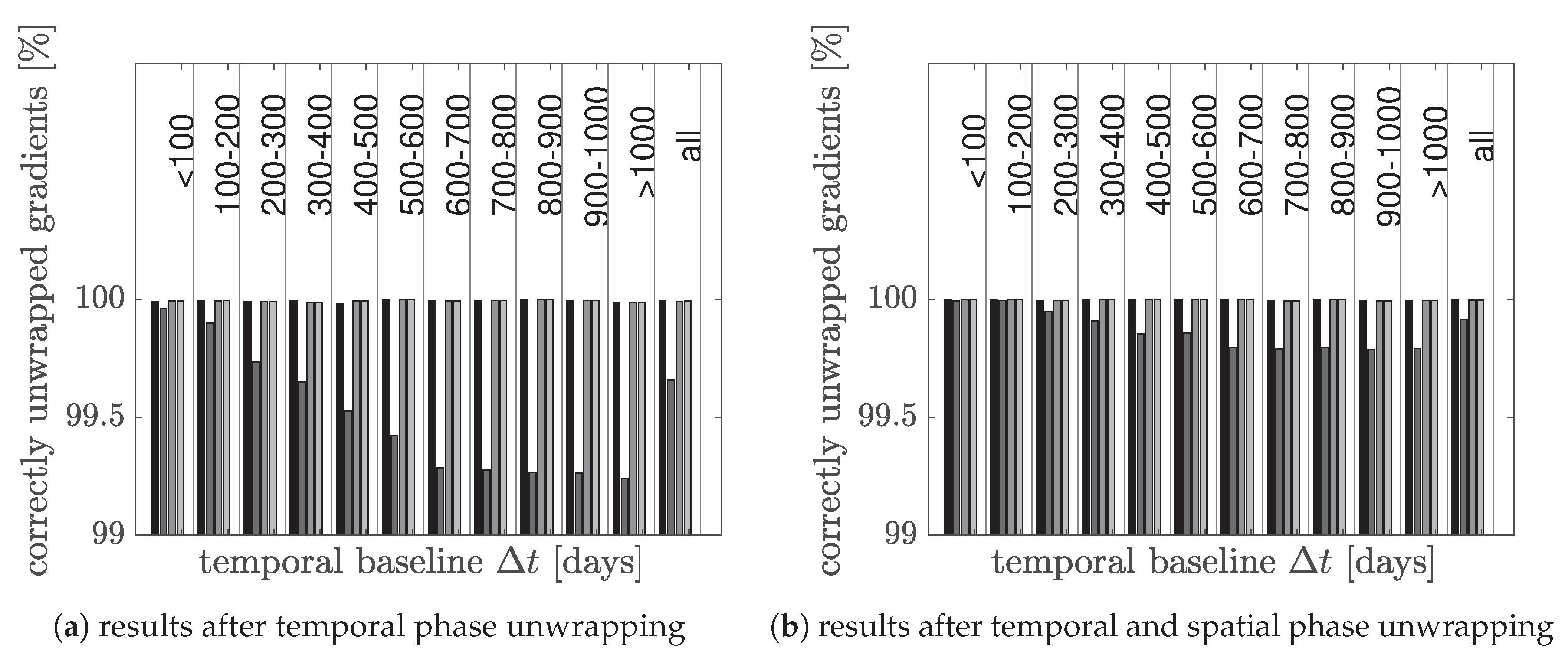
To analyze the phase unwrapping process in some more detail, a D-InSAR stack is simulated based on the ERS 1/2 configuration in time and space. Therefore, 64 SAR images from May 1992 to December 2000 are used which cover the test region of the Lower-Rhine-Embayment. The test region was restricted to 401 times 401 pixels. The whole workflow for generating the simulated interferometric phases is shown in Figure 5.

In the center of the test region, a ground settlement depression is simulated with respect to the first SAR image. The deformation consists of a linear trend. The deformation velocity is restricted to a range from 8 to 12 cm/yr and it reaches a dimension from 120 to 240 pixels. In addition to the deformation, a topographical error is modeled. This topographical error reaches values from –5 to 40 $\mathrm{m}$. To make the simulation more realistic a noise per SAR image is added which is assumed to be independent and identical distributed with a standard deviation of $0.4$ rad. With respect to the SBAS method, 161 interferograms are generated, see the corresponding temporal triangulation already shown in Figure 3. Filtering operations that are applied individually to each interferogram, such as the multilooking, cause the real data to be inconsistent over time. Therefore, one additional noise per interferogram is added depending on the unbiased coherence [28]. The corresponding coherence values are extracted from the ERS 1/2 real data set. With this coherence-based noise, the noise is set into dependency on the temporal and spatial baseline. Larger baselines create a lower coherence value and thus an increased noise.

The coherence values are also used to extract the so-called stable pixels. Pixels are defined as stable if they have a coherence value greater or equal to 0.7 in at least $80\%$ of the interferograms. Within the 401 times 401 large test region there are m = 15,347 stable pixels defining n = 45,842 arcs and r = 30,496 triangles. Figure 6a shows the simulated phases of the stable pixels in the test region for one interferogram. Due to the periodicity of the signal, the phase can only be measured from $-\pi$ to $\pi$, see Figure 6b.

4.2. EMCF vs. MCF

The MCF and the EMCF algorithms are applied to the simulated D-InSAR stack. To find the optimal motion model, the search area is chosen in a range from $-8$ cm/yr to 8 cm/yr with a step width of $0.5$ cm/yr for the deformation velocity variation $v_{∆x_{kl}}$ and in a range from $-50$ $\mathrm{m}$ to 50 $\mathrm{m}$ with a step width of 5 $\mathrm{m}$ for the error of the scene topography $∆h_{∆x_{kl}}$. For every possible ($v_{∆x_{kl}},∆h_{∆x_{kl}}$)-pair the modified observations are estimated and the corresponding temporal LP is solved. The pair which minimizes the cost function is chosen as optimal.

Figure 7 shows the results of the unwrapped phase gradients. The figure presents the percentage of correctly unwrapped phase gradients depending on the temporal baseline. The black bars show the results of the EMCF algorithm and the gray bars show the results of the MCF algorithm without exploiting the temporal relationship between the interferograms. It can be seen that the inclusion of the temporal phase unwrapping results in a higher percentage of correctly unwrapped phase gradients which confirms the findings of [5]. For every interferogram, even for the ones with a larger baseline and therefore with a higher noise level, nearly 100% of phase gradients are unwrapped correctly.

4.3. Estimation of the Motion Model

The estimation of the optimal motion model during the temporal phase unwrapping is an important step. Considering the spatial arc $∆x_{kl}$, the motion model includes the unknown deformation velocity variation $v_{∆x_{kl}}$ and the error of the scene topography $∆h_{∆x_{kl}}$. This model is used to estimate the modified observations ${\mathit{\chi }}_{∆x_{kl}}^{\mathsf{\Delta }\mathit{t}}$, cf. (24) which are inserted into the temporal LP, described in (25) to (27). The optimal motion model is estimated in an iterative search process. Therefore, the temporal LP is solved for each predefined ($v_{∆x_{kl}}$, $∆h_{∆x_{kl}}$)-pair and the one that causes the minimal cost value $C_{\min }$ is set as optimal. However, this procedure has some disadvantages. It is not straightforward how the search space and the step width should be efficiently selected. With a greater search space and smaller step width the complexity grows. Moreover, due to the discrete optimization function the solution is typically not unique. Since it is assumed that the deformation velocity variation and the error of the scene topography between adjacent pixels is rather small, the parameters that are closest to zero are defined as optimal.

To avoid this iterative search process with the involved solution of the LP in each search step, an alternative way is proposed here. The so-called ensemble phase coherence (EPC) [29] gives a value for the quality of the estimated model. For the arc $∆x_{kl}$ it is defined as

$$\begin{array}{c}\hfill EPC(v_{∆x_{kl}},∆h_{∆x_{kl}})=\left|\frac{{\displaystyle \sum _{\forall ∆t_{\alpha \beta }\in {\mathcal{N}}^{\prime }}}{e}^{i({\psi }_{∆x_{kl}}^{∆t_{\alpha \beta }}-\mathit{M})}}{n^{\prime }}\right|\end{array}$$

(28)

with the M from (20) which depends on the parameters $v_{∆x_{kl}}$ and $∆h_{∆x_{kl}}$. The EPC function is continuous with values between zero and one. A value of zero means that model and observation do not fit and a value of one means that model and observation fit optimal. With a higher noise level the maximum value of the function decreases and it gets difficult to find the global maximum. However, the idea is to define this ($v_{∆x_{kl}},∆h_{∆x_{kl}}$)-pair as optimal which maximizes the EPC, equal to [1].

Three different methods are tested to find the global maximum: the Nelder–Mead method [30], a grid search approach and simulated annealing [31]. Some of them need a starting point which results from a two-step weighted least squares adjustment [29].

Application to Simulated Data

To examine the three search methods and to check whether maximizing the EPC is a possible alternative to the conservative search process to minimize the costs of the temporal LP, two spatial gradients of the simulated D-InSAR stack are analyzed more closely. The arcs are chosen near the simulated settlement depression. Figure 8a,c show the discrete and iterative solved cost function values resulting from the temporal LP. It becomes obvious that there are several minima with a function value of 0. Since it is supposed that the optimum parameters should be as close to zero as possible, the black triangles indicate the optimum. For both arcs, the estimated parameters are very close to the reference shown as black stars. However, as the solution is not unique, it is possible that there are other optimal parameters that would fit even better to the reference.

Figure 8b,d show the EPC function for an equivalent range of values. The results of the individual search methods are marked in different symbols. The gray square is the maximum found by Nelder–Mead, the gray triangle is the maximum found by the grid search algorithm and the light gray point is the result of using simulated annealing. For the grid search, the search area is chosen analogous to the iterative cost minimization task. The black dot indicates the initial solution from the two-step weighted least squares adjustment necessary for the Nelder–Mead method and simulated annealing. Looking first at arc 1 in Figure 8b, it becomes clear that all three search methods work and produce approximately identical results. Simulated annealing finds the maximum EPC value which of all methods fits best to the reference parameters. For arc 2, considered in Figure 8d, it becomes clear that the Nelder–Mead method is not able to find the global maximum. Starting from the initial solution, it stops at a local maximum. The estimated parameters using grid search and simulated annealing are very consistent with the minimum of the cost value in Figure 8c and therefore fits well to the reference.

In order to investigate the influence of the differently estimated parameters on the phase unwrapping results, Figure 9 shows an overall comparison. First, Figure 9a shows the results after the temporal phase unwrapping without considering the spatial information. The figure shows the percentage of correctly unwrapped phase gradients in dependence of the temporal baseline. The different gray levels refer to the different methods for estimating the motion model. The black bars are the results of the conventional way by minimizing the costs of the temporal LP in an iterative search process. The gray bars are the results of the alternative way by maximizing the EPC. Dark gray symbolizes the results using the Nelder–Mead method, middle gray using the grid search algorithm and light gray using simulated annealing. All results represent a valid solution after the definition of the phase unwrapping problem. The results differ only in the choice of motion model parameters. The above statements can be confirmed on the basis of Figure 9a. Maximizing the EPC using the Nelder–Mead method does not work well. However, if the grid search method or simulated annealing is used to maximize the EPC, it can be seen that the results are comparable to the conventional method, shown as black bars. Almost all gradients can be unwrapped correctly by the temporal phase unwrapping alone. The last few percentages are reached after applying the spatial phase unwrapping, see Figure 9b. Some errors caused by wrongly estimated motion model parameters using the Nelder–Mead method can still be fixed by the spatial phase unwrapping, but the result remains that Nelder–Mead is the worst compared to the other methods.

Maximizing the EPC function using the grid search method or simulated annealing is a good alternative to find a suitable motion model. The conventional method has the disadvantage that the discrete function may consist of a set of potential solutions and especially if the search area is unknown or very large, the method results in a long run time as the temporal phase unwrapping problem has to be solved sequentially for each ($v_{∆x_{kl}}$, $∆h_{∆x_{kl}}$)-pair. In this simulation, the cost function was evaluated sequentially in 693 steps. For a single arc the temporal LP has to be solved 693 times. Compared to this, the temporal LP only needs to be solved once with the alternative method resulting in a reduced run time of up to 1/10.

Simulated annealing provides the highest EPC values in all cases and is a very robust and efficient method. Therefore, it will be used in the following. Maximizing the EPC using simulated annealing is defined as the alternative approach and the sequential solving of the temporal LP for each ($v_{∆x_{kl}}$, $∆h_{∆x_{kl}}$)-pair the conventional approach.

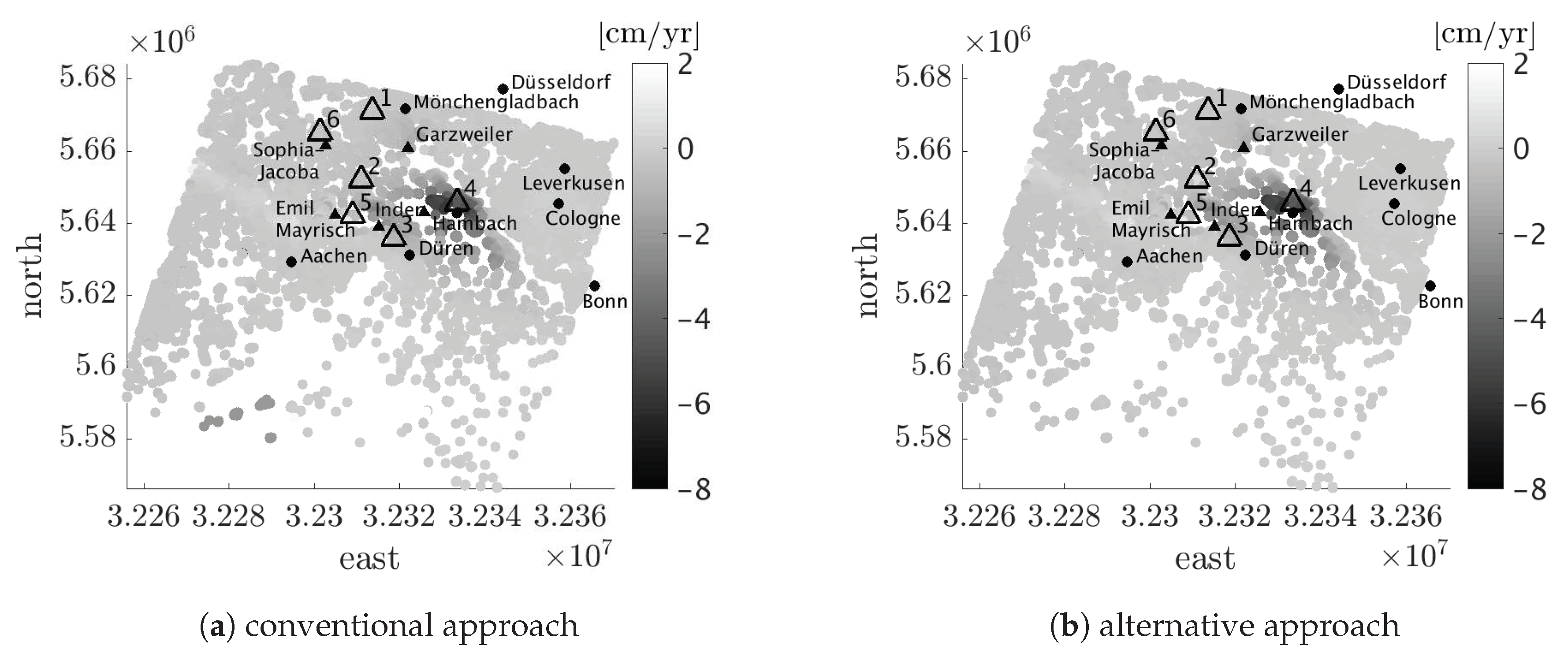
5. Application to Real Data

In order to verify the performance of the described methods, both approaches, the alternative and the conventional approach, are applied to real data. The considered data set consists of the previously mentioned 64 SAR images collected by ERS 1/2. These data cover the Lower-Rhine-Embayment from May 1992 to December 2000 and they are stacked together to 161 D-InSAR images. The temporal data distribution is already shown in Figure 3. Again, pixels are defined as coherent if they have a coherence value greater or equal to 0.7 in at least 80% of the interferograms. For the whole ERS 1/2 scene this is the case for n = 143,213 pixels defining m = 429,336 arcs and r = 286,124 triangles.

Characteristic for the Lower-Rhine-Embayment are the mining regions. The coal mine Sophia-Jacoba in the mining region Erkelenz and the coal mine Emil Mayrisch in the mining region Aachen had been extracted underground until 1992 and 1997, respectively [4]. The resulting groundwater rise in the pits caused the Earth’s surface to lift again. In contrast, the three still active open-cast mines Garzweiler, Hambach and Inden in the Rhineland brown coal mining area are causing subsidence of the Earth’s surface. The aim is to detect these deformations with the help of a multitemporal D-InSAR analysis.

All pre-processing steps from the coregistration of the individual SAR images to the wrapped differential interferograms are done with the Remote Sensing Software Graz (RSG). To improve the ground deformation capability an effective noise-filtering and an efficient interferogram selection procedure is integrated according to [27]. For better analysis, the phase unwrapping step is performed twice externally in MATLAB^©. The unwrapped phase gradients are included in RSG again for the final SBAS analysis which results in a mean deformation velocity map shown in Figure 10.

Since the phase gradients represent temporal and spatial double differences, both a temporal and a spatial reference must be chosen to overcome the datum defect. The spatial reference is a point in Cologne, since it can be assumed that the region in Cologne is stable. The first SAR observation in May 1992 is chosen as temporal reference.

Figure 10a shows the results using the conventional approach to estimate the motion model parameters and Figure 10b shows the results using the alternative way. First of all, both analyses show that the Earth’s surface around the still active open-cast mines Garzweiler and Hambach subsides in a range from $-6$ to $-8$ cm/yr. On the contrary, closing the mines Sophia-Jacoba in 1997 and Emil Mayrisch in 1992 causes the Earth’s surface to rise by a few cm/yr. On a more detailed examination of the results, the figures show isolated irregularities and jumps that may indicate a phase unwrapping error. It becomes clear that the poor redundancy at the borders causes problems. Especially with the conventional method there are jumps of ± 2 cm/yr in the south.

In Figure 11 deformation time series of five different points inside each of the six highlighted regions in Figure 10 are examined in more detail and compared with the closest leveling point. Therefore, the leveling data measured by GeoBasis NRW in a four-year cycle are used and evaluated in an individual adjustment following [32]. When comparing the two data sets, the problem of different spatial and temporal resolution and the problem of different temporal reference points occur. Since all examined points are generally within a radius of about 300 $\mathrm{m}$, it is assumed that they should show a similar behavior, since the deformation should not change abruptly. Correctly, it would have to be taken into account that using D-InSAR only movements in line-of-sight can be observed. However, the leveling data refer to vertical height changes. Since only ERS 1/2 data of descending orbits are available for the work presented here, the separation into a horizontal and a vertical component is not possible and it has to be assumed that no horizontal movement takes place. The time offset is compensated by linearly interpolating the leveling data piecewise over time according to [33]. For each coherent pixel, a local offset is calculated using a weighted average. Figure 11 shows the corresponding deformation time series after applying the local offset. The results of the D-InSAR analysis using the conventional method are shown as black triangles and using the alternative method as light gray points. The leveling results are plotted as black squares. The reader is reminded that the vertical axes of the plots were chosen differently since the examined points show differently strong motions.

The pixels in test region 1 are located in Mönchengladbach, a very stable area where no large movements should take place, see Figure 11a. However, it is clearly visible that the conventional method indicates a strong uplift at one pixel. Looking at the associated phase gradients that contain this pixel, it becomes clear that the wrong motion model parameters were estimated. The mean deformation velocities are too extreme. For this special pixel, the alternative method works better. The estimated motion model parameters fit better to the adjacent pixels and to the leveling data.

A comparable example can be seen in the second test region in Gevenich, Linnich near the active open-cast mine Garzweiler, see Figure 11b. Brown coal mining causes the Earth’s surface to subside by a few centimeters. However, one point shows an extreme decrease. In this case, the conventional method also fails and leads to incorrect motion model parameters at the associated phase gradients.

Figure 11c shows pixels in Jülich near the still-active open-cast mines Inden and Garzweiler. Again, there is a decrease and one pixel differs slightly from its neighboring pixels. The conventional method yields another slightly stronger decrease. However, this stronger decrease is also detected by the closest leveling point. Thus, the behavior deviates from the surrounding pixels, but fits better to the leveling results.

In the following, three examples are shown in which both methods work well and provide comparable results. Figure 11d examines pixels in Thorr next to the open-cast mine Garzweiler. There is a clear decrease of the Earth’s surface which is recorded nearly equally by both methods and fits well with the leveling results.

The pixels in test region 5 are located in Aldenhoven in the basin of the mining region Aachen, see Figure 11e. As already mentioned, coal had been mined there until 1992. This can be seen in the corresponding subsidence of the ground which, however, slowly weakened at the end of 2000. The subsequent rise in the groundwater level causes a renewed uplift which is already becoming apparent at the end of the D-InSAR data. Again, both methods provide identical results and agree with the leveling data.

The last considered test region is located in Wassenberg near the mining region Erkelenz where coal mining took place until 1997. The resulting subsidence is reflected much more strongly in the D-InSAR data than in the leveling data. The following flooding of the mine galleries leads to a renewed uplift of the Earth’s surface which becomes clearly visible in the temporally more highly resolved D-InSAR data in 2000. Once again, both methods lead to nearly the same motion model.

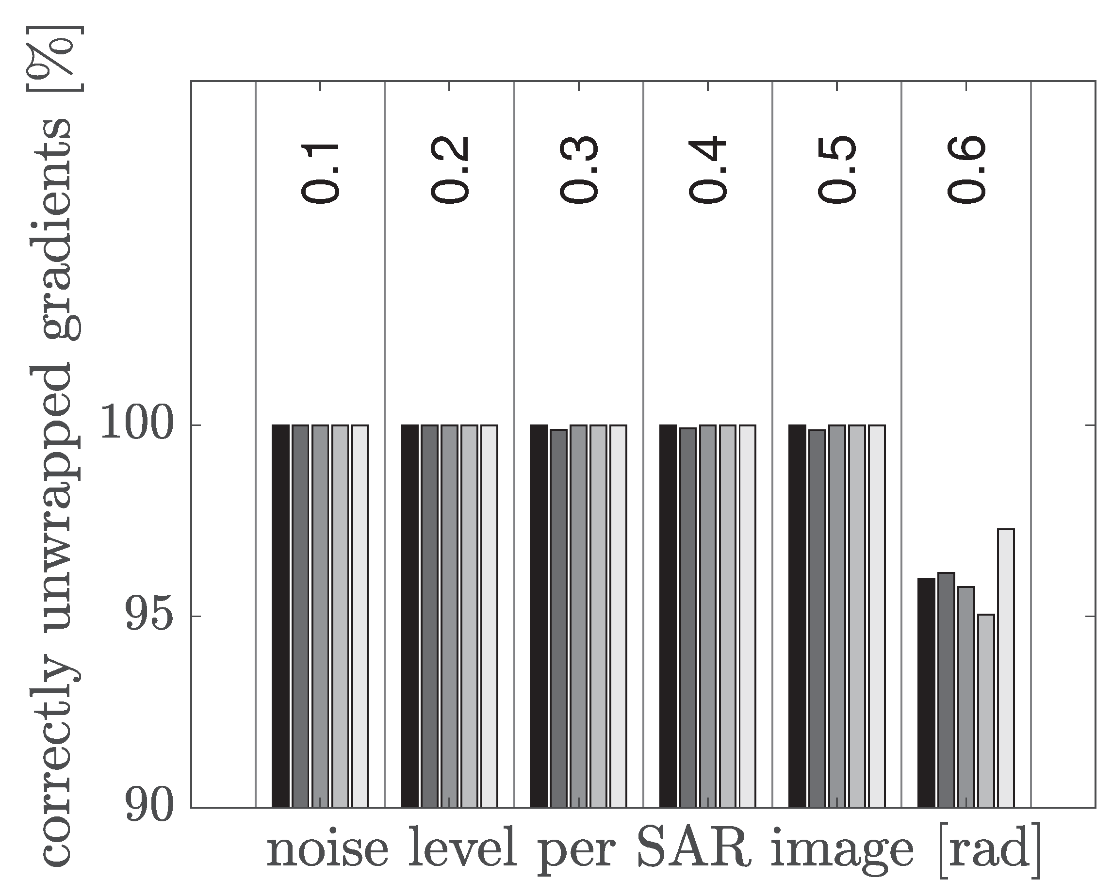
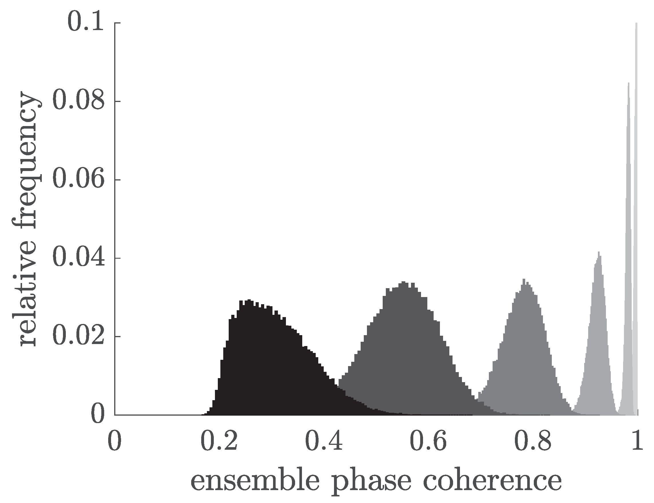
6. Discussion: Analysis for Different Scenarios

For a more general conclusion, the studies are repeated for different simulated scenarios. The noise level per SAR image varies from 0.1 to $0.6$ rad. Figure 12 shows the percentage of correctly unwrapped gradients for the entire D-InSAR stack depending on the noise level. For a noise level till $0.5$ rad the results described above are confirmed. For a noise level of $0.6$ rad it looks different. In this case, the search algorithm with Nelder–Mead, shown as dark gray bars, provides the best results. For a higher noise level, the EPC values are very small and there is no significant global maximum. Figure 13 shows the relative frequency of the occurring EPC values found by simulated annealing for the different noise levels. The darker the color of the histogram, the higher the noise. Furthermore, Figure 14 shows exemplary for one spatial arc of the simulated D-InSAR stack with a noise level of $0.6$ rad the iteratively solved cost function (Figure 14a) and the EPC (Figure 14b). It is obvious that the EPC reaches very small values and that there is no significant maximum. Although simulated annealing and the grid search method find the global maximum, the reference values are at a slightly smaller EPC value with motion model parameters near 0. Since there are several local maxima, the Nelder–Mead algorithm ends near the starting solution, which in this case fits better to the reference.

With a higher noise level and thus smaller EPC values, the estimated motion model cannot be reliably estimated. In such cases, it is better to use a motion model that corresponds to a local maximum close to 0 instead of using an extreme motion model, which is very unreliable and may lead to phase unwrapping errors. Based on this conclusion, the idea is to use a modified search algorithm. This search algorithm relies on the results of simulated annealing as long as the EPC value is above a certain threshold and for smaller values, it is assumed that the motion model could not be estimated reliably and instead, the local maximum around 0 is taken using the Nelder–Mead method. For this simulation, the threshold is set to 0.3 rad based on the histogram in Figure 13.

For the arc analyzed in Figure 14b, the optimum point found by this modified algorithm is marked as a white triangle that fits better to the reference as the solution found by simulated annealing. A corresponding overall result of the percentage of correctly unwrapped phase gradients is shown as white bars in Figure 12. For a noise level till $0.5$ rad the results are identical to simulated annealing and the grid search algorithm. However, with a noise level of $0.6$ rad an improvement can be seen, also with respect to the conventional way by minimizing the costs of the temporal LP in an iterative search process.

Considering the real ERS 1/2 data set, the resulting EPC values using simulated annealing are only in 0.1% of cases below the selected threshold of 0.3 rad. So in most cases, simulated annealing will estimate reliable motion model parameters. However, if the data is extremely noisy, it would be better to use the modified search algorithm.

7. Conclusions

This paper focuses on the three-dimensional EMCF algorithm. The inclusion of the temporal relationship between the interferograms results in a higher percentage of correctly unwrapped phase gradients. However, the disadvantage is that the motion model parameters $v_{∆x_{kl}}$ and $∆h_{∆x_{kl}}$ which are necessary during the temporal phase unwrapping, have to be estimated in an iterative search process.

Therefore, a special search space is defined and divided into certain step widths. For each ($v_{∆x_{kl}}$, $∆h_{∆x_{kl}}$)-pair the temporal LP is solved searching for the minimal cost value. The problem is that the choice of the search space is not straightforward and should, therefore, be as large and fine as possible. This results in very long run times. Moreover, due to the discrete optimization function, the minimum is not necessarily unique.

This paper presents an alternative way to estimate the motion model by maximizing the continuous EPC function. Different optimization algorithms are compared to find the global maximum. Applied to the simulated data, it could be shown that this alternative way works. When high noise is expected, a modified approach combining simulated annealing and Nelder–Mead is recommended. Since the temporal LP only has to be solved once and not iteratively, the alternative method is much faster in run time and is thus well suited for the processing of large data sets.

When applied to real data, the alternative method has also shown its efficiency. Compared to leveling data, the crucial movements are correctly detected. In some pixels, it could even be shown that the alternative method estimates a better motion model than the conventional method.

References

1. Ferretti, A.; Prati, C.; Rocca, F. Permanent Scatterers in SAR Interferometry. IEEE Trans. Geosci. Remote Sens. 2001, 39, 8–20. [Google Scholar] [CrossRef]
2. Berardino, P.; Fornaro, G.; Lanari, R.; Sansosti, E. A New Algorithm for Surface Deformation Monitoring Based on Small Baseline Differential SAR Interferograms. IEEE Trans. Geosci. Remote Sens. 2002, 40, 2375–2383. [Google Scholar] [CrossRef]
3. Ferretti, A.; Fumagalli, A.; Novali, F.; Prati, C.; Rocca, F.; Rucci, A. A New Algorithm for Processing Interferometric Data-Stacks: SqueeSAR. IEEE Trans. Geosci. Remote Sens. 2011, 49, 3460–3470. [Google Scholar] [CrossRef]
4. Boje, R.; Gstirner, W.; Schuler, D.; Spata, M. Leitnivellements in Bodenbewegungsgebieten des Bergbaus-Eine Langjährige Kernaufgabe der Landesvermessung in Nordrhein-Westfalen. NÖV NRW 2008, 3, 33–42. [Google Scholar]
5. Pepe, A.; Lanari, R. On the Extension of the Minimum Cost Flow Algorithm for Phase Unwrapping of Multitemporal Differential SAR Interferograms. IEEE Trans. Geosci. Remote Sens. 2006, 44, 2374–2383. [Google Scholar] [CrossRef]
6. Pritt, M.D. Phase Unwrapping by Means of Multigrid Techniques for Interferometric SAR. IEEE Trans. Geosci. Remote Sens. 1996, 34, 728–738. [Google Scholar] [CrossRef]
7. Flynn, T.J. Two-Dimensional Phase Unwrapping with Minimum Weighted Discontinuity. JOSA A 1997, 14, 2692–2701. [Google Scholar] [CrossRef]
8. Eineder, M.; Hubig, M.; Milcke, B. Unwrapping Large Interferograms Using the Minimum Cost Flow Algorithm. In Proceedings of the IGARSS ’98, Sensing and Managing the Environment, 1998 IEEE International Geoscience and Remote Sensing, Symposium Proceedings, (Cat. No.98CH36174), Seattle, WA, USA, 6–10 July 1998; Volume 1, pp. 83–87. [Google Scholar] [CrossRef]
9. Ghiglia, D.C.; Pritt, M.D. Two-Dimensional Phase Unwrapping: Theory, Algorithms and Software; WileyBlackwell: Hoboken, NJ, USA, 1998. [Google Scholar]
10. Ferretti, A.; Monti-Guarnieri, A.; Prati, C.; Rocca, F.; Massonnet, D. InSAR Principles: Guidelines for SAR Interferometry Processing and Interpretation, Part C: InSAR processing: A mathematical approach; ESA: Paris, France, 2007. [Google Scholar]
11. Fornaro, G.; Pauciullo, A.; Reale, D. A Null-Space Method for the Phase Unwrapping of Multitemporal SAR Interferometric Stacks. IEEE Trans. Geosci. Remote Sens. 2011, 49, 2323–2334. [Google Scholar] [CrossRef]
12. Tribolet, J. A New Phase Unwrapping Algorithm. IEEE Trans. Acoust. Speech Signal Process. 1977, 25, 170–177. [Google Scholar] [CrossRef]
13. Goldstein, R.M.; Zebker, H.A.; Werner, C.L. Satellite Radar Interferometry: Two-Dimensional Phase Unwrapping. Radio Sci. 1988, 23. [Google Scholar] [CrossRef]
14. Zebker, H.A.; Lu, Y. Phase Unwrapping Algorithms for Radar Interferometry: Residue-Cut, Least-Squares, and Synthesis Algorithms. JOSA A 1998, 15, 586–598. [Google Scholar] [CrossRef]
15. Ghiglia, D.C.; Romero, L.A. Robust Two Dimensional Weighted and Unweighted Phase Unwrapping That Uses Fast Transforms and Iterative Methods. JOSA A 1994, 11, 107–117. [Google Scholar] [CrossRef]
16. Costantini, M. A Phase Unwrapping Method Based on Network Programming. In ERS SAR Interferometry; European Space Agency - Publications; ESA: Zurich, Switzerland, 1997; Volume 406, pp. 261–272. [Google Scholar]
17. Costantini, M.; Rosen, P. Generalized Phase Unwrapping Approach for Sparse Data. In Proceedings of the IEEE 1999 International Geoscience and Remote Sensing Symposium, IGARSS’99 (Cat. No.99CH36293), Hamburg, Germany, 28 June–2 July 1999; Volume 1, pp. 267–269. [Google Scholar] [CrossRef]
18. Hooper, A.; Zebker, H.A. Phase unwrapping in three dimensions with application to InSAR time series. JOSA A 2007, 24, 2737–2747. [Google Scholar] [CrossRef] [PubMed] [Green Version]
19. Shanker, A.P.; Zebker, H. Edgelist Phase Unwrapping Algorithm for Time Series InSAR Analysis. JOSA A 2010, 27, 605–612. [Google Scholar] [CrossRef] [PubMed]
20. Costantini, M.; Malvarosa, F.; Minati, F. A General Formulation for Redundant Integration of Finite Differences and Phase Unwrapping on a Sparse Multidimensional Domain. IEEE Trans. Geosci. Remote Sens. 2011, 50, 758–768. [Google Scholar] [CrossRef]
21. Schrijver, A. Theory of Linear and Integer Programming; John Wiley & Sons, Inc.: New York, NY, USA, 1986. [Google Scholar]
22. Dantzig, G. Linear Programming and Extensions; Princeton University Press: Princeton, NJ, USA, 1963. [Google Scholar]
23. Karmarkar, N. A New Polynomial-Time Algorithm for Linear Programming. Combinatorica 1984, 4, 373–395. [Google Scholar] [CrossRef]
24. Wilson, R.J. Introduction to Graph Theory; John Wiley & Sons, Inc.: New York, NY, USA, 1986. [Google Scholar]
25. Fulkerson, D.R. An Out-of-Kilter Method for Minimal-Cost Flow Problem. J. Soc. Ind. Appl. Math. 1961, 9, 18–27. [Google Scholar] [CrossRef]
26. Bertsekas, D.P.; Tseng, P. Relaxation Methods for Minimum Cost Ordinary and Generalized Network Flow Problems. Oper. Res. 1988, 36, 93–114. [Google Scholar] [CrossRef] [Green Version]
27. Pepe, A.; Yang, Y.; Manzo, M.; Lanari, R. Improved EMCF-SBAS Processing Chain Based on Advanced Techniques for the Noise-Filtering and Selection of Small Baseline Multi-Look DInSAR Interferograms. IEEE Trans. Geosci. Remote Sens. 2015, 53, 4394–4417. [Google Scholar] [CrossRef]
28. Lee, J.S.; Hoppel, K.W.; Mango, S.A.; Miller, A.R. Intensity and Phase Statistics of Multilook Polarimetric and Interferometric SAR Imagery. IEEE Trans. Geosci. Remote Sens. 1994, 32, 1017–1028. [Google Scholar] [CrossRef]
29. Zhang, K.; Li, Z.; Meng, G.; Dai, Y. A Very Fast Phase Inversion Approach for Small Baseline Style Interferogram Stacks. ISPRS J. Photogramm. Remote Sens. 2014, 97, 1–8. [Google Scholar] [CrossRef]
30. Nelder, J.A.; Mead, R. A Simplex Method for Function Minimization. Comput. J. 1965, 7, 308–313. [Google Scholar] [CrossRef]
31. Kirkpatrick, S.; Gelatt, C.D.; Vecchi, M.P. Optimization by Simulated Annealing. Science 1983, 220, 671–680. [Google Scholar] [CrossRef] [PubMed]
32. Halsig, S.; Ernst, A.; Schuh, W.D. Ausgleichung von Höhennetzen aus mehreren Epochen unter Berücksichtigung von Bodenbewegungen. Z. Für Geod. Geoinf. Landmanag. 2013, 4, 288–296. [Google Scholar]
33. Esch, C.; Köhler, J.; Gutjahr, K.; Schuh, W.D. 25 Jahre Bodenbewegungen in der Niederrheinischen Bucht–Ein kombinierter Ansatz aus D-InSAR und amtlichen Leitnivellements. Z. Für Geod. Geoinf. Landmanag. 2019, 3, 173–186. [Google Scholar]
Figure 1. Spatial Delaunay triangulation for an example of four pixels. To ensure that the solution is rotation-free, the sum of the unwrapped phase gradients in one triangle has to be zero.
Remotesensing 11 02295 g001
Figure 2. Dual graph of Figure 1. The constraints of the primal problem define the new nodes with node potential b. The arcs connect these nodes by cutting the arcs of the primal graph.
Remotesensing 11 02295 g002
Figure 3. Temporal triangulation related to the small baseline subset (SBAS) method. The white dots represent the individual SAR scenes at the individual acquisition times with corresponding orthogonal spatial baseline relating to the master scene. The black lines represent the interferograms.
Remotesensing 11 02295 g003
Figure 4. Temporal relationship for one spatial arc. The thickly marked line is analysed in time. To ensure that the solution is rotation-free in the temporal plane, the sum of the three phase gradients has to be zero.
Remotesensing 11 02295 g004
Figure 5. Workflow for generating simulated interferometric phases. The simulated SAR images consist of a ground settlement, a topographical error and a noise part. On this basis, interferograms are generated, which in turn are provided with noise.
Remotesensing 11 02295 g005
Figure 6. Coherent pixels of simulated ground settlement depression for one interferogram with a temporal baseline of t α β = 315 days and an orthogonal spatial baseline of b , α β = −217.645 m.
Remotesensing 11 02295 g006
Figure 7. Percentage of correctly unwrapped phase gradients depending on the temporal baseline. The results of the extended minimum cost flow (EMCF) algorithm are shown as black bars. The gray bars represent the results of the MCF algorithm without considering the temporal information.
Remotesensing 11 02295 g007
Figure 8. Cost values and corresponding ensemble phase coherence (EPC) values for two simulated spatial gradients. The black triangles in the left figures symbolize the optimal point resulting from the iterative search process where the costs of the temporal linear program (LP) are minimized. For comparison, the black star is the reference solution. The other symbols in the right figures represent the optimum point from maximizing the EPC. The gray square is obtained using the Nelder–Mead method, the gray triangle using the grid search process and the light gray point using simulated annealing. The black point represents the starting solution.
Remotesensing 11 02295 g008
Figure 9. Percentage of correctly unwrapped phase gradients depending on the temporal baseline. The motion model is estimated with different approaches. The black bars show the results of the conventional way by minimizing the costs of the temporal LP in an iterative search process. The dark gray bars show the results using the Nelder–Mead method to estimate the motion model by maximizing the EPC, the middle gray bars when using the grid search method and the light gray bars when using simulated annealing.
Remotesensing 11 02295 g009
Figure 10. Mean deformation velocity map of the Lower-Rhine-Embayment based on ERS 1/2 data from May 1992 to December 2000. The deformation model is estimated using the conventional and the alternative approach. The highlighted test regions 1 to 6 are examined in more detail as a time series in Figure 11.
Remotesensing 11 02295 g010
Figure 11. Deformation time series of five points lying in each of the six highlighted test region shown in Figure 10. The black triangles are the results using the conventional approach and the light gray points are the results using the alternative way. For comparison the black squares indicate the data from the closest leveling point.
Remotesensing 11 02295 g011
Figure 12. Percentage of correctly unwrapped phase gradients depending on the noise level. The motion model is estimated with different approaches, see different gray levels already described in Figure 9. The additional white bars show the results using a modified search algorithm combining simulated annealing and the Nelder–Mead method.
Remotesensing 11 02295 g012
Figure 13. Relative frequency of occuring EPC values using simulated annealing. The darker the color of the histogram, the higher the noise level. It varies from 0.1 rad to 0.6 rad.
Remotesensing 11 02295 g013
Figure 14. Cost values and corresponding EPC values for one spatial arc of the simulated D-InSAR stack with a noise level of 0.6 rad. The black triangle in the left figure shows the results of the conventional way. The black star is the reference solution. The gray square in the right figure shows the results using the Nelder–Mead method for maximizing the EPC, the gray triangle when using the grid search method, the light gray point when using simulated annealing and the white triangle when using a modified search algorithm combining simulated annealing and the Nelder–Mead method. The black point represents the starting solution which is necessary for some algorithms.
Remotesensing 11 02295 g014