Article

Integration of a Landsat Time-Series of NBR and Hydrological Modeling to Assess Pinus pinaster Aiton. Forest Defoliation in South-Eastern Spain

by
Antonio Jesús Ariza Salamanca
1,*,†,
Rafael María Navarro-Cerrillo
1,†,
Francisco J. Bonet-García
2,
Ma José Pérez-Palazón
3 and
María J. Polo
3
1
Department of Forestry Engineering, Laboratory of Silviculture, dendrochronology and climate change. DendrodatLab-ERSAF, Andalusian Institute for Earth System Research, University of Cordoba, Campus de Rabanales, Crta. IV, km. 396, E-14071 Córdoba, Spain
2
Department of Ecology, University of Cordoba, Campus de Rabanales, Crta. IV, km. 396, E-14071 Córdoba, Spain
3
Department of Hydraulic Engineering, Laboratory of River Dynamics and Hydrology, Andalusian Institute for Earth System Research, University of Cordoba, Campus de Rabanales, Crta. IV, km. 396, E-14071 Córdoba, Spain
*
Author to whom correspondence should be addressed.
Co-first authors.
Remote Sens. 2019, 11(19), 2291; https://doi.org/10.3390/rs11192291
Submission received: 1 September 2019 / Revised: 24 September 2019 / Accepted: 29 September 2019 / Published: 30 September 2019

Abstract

:
Climate change is increasing the vulnerability of Mediterranean coniferous plantations. Here, we integrate a Landsat time series with a physically-based distributed hydrological model (Watershed Integrated Management in Mediterranean Environments—WiMMed) to examine spatially-explicit relationships between the mortality processes of Pinus pinaster plantations and the hydrological regime, using different spectral indices of vegetation and machine learning algorithms. The Normalized Burn Ratio (NBR) and Moisture Stress Index (MSI) show the highest correlations with defoliation rates. Random Forest was the most accurate model (R2 = 0.79; RMSE = 0.059), showing a high model performance and prediction. Support vector machines and neural networks also demonstrated a high performance (R2 > 0.7). The main hydrological variables selected by the model to explain defoliation were potential evapotranspiration, winter precipitation and maximum summer temperature (lower Out-of-bag error). These results show the importance of hydrological variables involved in evaporation processes, and on the change in the spatial distribution of seasonal rainfall upon the defoliation processes of P. pinaster. These results underpin the importance of integrating temporal remote sensing data and hydrological models to analyze the drivers of forest defoliation and mortality processes in the Mediterranean climate.

Graphical Abstract

1. Introduction

Mediterranean Basin forests have undergone a severe and accelerated process of historical degradation [1]. To protect the soil against erosion and to restore watersheds, during the second half of the 20th century ca. 3.5 million ha (ca. 8.6 million acres or 13,513 square miles) were reforested in Spain, the area occupied by conifers representing 78.3% of the total reforested area and 54.5% of the national area covered by conifers [2]. Usually, pine plantations present a set of structural problems (e.g., regularity, coetaneity (being contemporaneous), and high density), which are associated with a lower resilience capacity of such forests [3].
The rise in temperature and increased frequency of severe droughts predicted for the near future [4] will increase the vulnerability of Mediterranean coniferous plantations, ultimately affecting their growth, vigor and long-term persistence [5,6,7]. Declining radial growth and increased mortality rates have been described for drought-prone forests throughout the world [8], leading to widespread tree mortality across many forest biomes [9], due to induction of stomatal closure, catastrophic xylem embolism of the vascular system, or hydraulic failure related to soil water availability [10]. However, the estimation of the soil water available to plants using meteorological information is very complex, due to the large number of processes involved in the soil–water balance. Moreover, field measurement of these processes is expensive, labor-intensive, and often limited in temporal scope and spatial scale [11]. For this purpose, most studies have used hydrological models to delineate the soil-hydrological cycle [12]; although, there is a limited number of studies where hydrological models were used in the context of forest decline analysis, particularly in forest plantations [13]. One of these models used in this study, the Watershed Integrated Management in Mediterranean Environments (WiMMed) model, is a physically-based, distributed hydrological model, which has been used to obtain a spatial interpolation of the meteorological variables and the physical modeling of the water in the soil. This model was specifically developed for surface hydrology studies in Mediterranean climates [14].
Forest decline related to droughts and pathogen outbreaks appears to be increasing in various forest ecosystems [15]. The use of remote sensing data for the early detection of these processes is critical to assess their impacts before more profound structural changes occur [16]. Defoliation is one of the most widely used parameters to monitor decline processes in forestry, thus its assessment has important implications for the estimation of vegetation status [17]. In this context, the Landsat program still offers both the temporal (16 days on average) and the spectral (seven reflectance bands covering the visible, near-infrared and shortwave-infrared wavelengths) capabilities necessary for ecological monitoring and the detection of change [18,19]. The canopies of pine plantations are generally homogeneous and spectrally uniform. For this reason, remote sensing is a useful approach for understanding the dynamics of these forests and their responses to natural disturbance [20]. Multispectral sensors have been successfully used to estimate biophysical variables in closed forest canopies [21]. However, due to the complexity of the estimation of biophysical variables at canopy level, several normalizing indices have been used to minimize any effects of the soil background and scattering processes caused by structural canopy properties [22]. Hence, defoliation measured using a time series of Vegetation Indices (VIs) at annual and sub-annual scales provides an opportunity for a timely detection of canopy changes related to forest decline [23].
Remotely-sensed and ancillary data used in heterogeneous landscapes can be non-normal, multi-model and categorical [24]. For this reason, non-parametric methods have gained heightened research interest in the last decade [25]. Thus, various advanced classification algorithms such as Random Forest (RF) [26], Support Vector Machines (SVMs) [27] and Neural Networks (NNs) [28] are some of the more-popular, non-parametric algorithms based on machine learning (ML) to extract tree species information from multi-sensor and multispectral remote sensing images due to their superior image handling capability [29]. In particular, RF is widely used for classifying multi- and hyperspectral data for plant species identification and classification [30], while, the application of SVM and ANN classification algorithms has been mainly explored in forest species classification using multispectral imagery [31]. Previous studies have used different ML methods in the context of forest decline analysis using VIs and climate data [32].
In the last decades, there has been an increase of interest in understanding the relationship between drought-induced forest decline and the spatiotemporal dynamics of water availability through the use of hydrological models [33]. However, to the best of our knowledge, the usefulness of VIs derived from Landsat data for the estimation of Pinus pinaster defoliation has not been investigated. There is also a lack of information on how machine-learning (ML) methods can perform on delineating forest defoliation processes in Mediterranean pine plantations [32].
Based on the experience of previous results [21,34] which investigated the use of Landsat for forest defoliation assessment in the same area, the objective of this study was to integrate information derived from long time-series of Landsat images and the hydrological model Watershed integrated Management (“WiMMed”) to assess the defoliation processes of Pinus pinaster Aiton plantations in Southern Spain. Our specific aims were: (i) To identify the most robust VIs obtained from Landsat temporal series for P. pinaster stands defoliation assessment at stands level; (ii) to identify hydrological variables trends using WiMMed, and provide a conceptual framework that explains the hydrologic stresses and factors causing defoliation in P. pinaster stands; (iii) to quantify the relationships between hydrological variables and VIs at the stand scale using machine-learning (ML) methods (RF; SVM and NNs), thereby identifying the main environmental variables related to forest defoliation processes; and (iv) to develop prediction models to forecast yearly defoliation for the study area based on the best environmental drivers. Our results present a novel approach to a rapid and effective assessment of defoliation on large forest areas, and addressing the main hydrological variables behind those processes. Large-scale mapping can help to develop an adaptive silviculture in even-aged pine stands under the current impacts of climate change in drought-prone areas.

2. Materials and Methods

2.1. Study Area

The study area is located in South-eastern Spain (Sierra de Baza, Granada-Andalusia (hereafter SB, 37°23′0″N, 2°50′0″W, elevation 800 to 1200 m) captured by Landsat path 200, row 34) (Figure 1), which has experienced contrasting pine mortality processes according to the Forest Health Andalusia Network in 2013 and increasing forward, related to locally intense droughts [5]. The pine plantations selected for study grow in an abrupt area at an elevation ranging from 1177 to 2062 m a.s.l., covering an area of 3080 ha (ca. 7611 acres). The mean annual temperature is 11.6 °C, and annual precipitation oscillates between 354 mm and 494 mm, concentrating mainly in winter (35%), and to a lesser extent in spring-fall (30%, Baza, Regional Climate Center, 1981–2017), corresponding to a Mediterranean semi-arid climate [35]. The annual average potential evapotranspiration (PET) is more than twice the average annual rainfall, presenting negative values between seven and eight months. The geological substrate is composed of phyllites and quartzites, with the most abundant soil types being leptosols and regosols on dolomites in naturally regenerated forests, and entisols and inceptisols on limestones in plantations. The forest stands in this region are mainly characterized by pine forest plantations (Pinus sylvestris L., Pinus nigra Arnold subsp. salzmannii (Dunal), Pinus pinaster Aiton and Pinus halepensis Mill.) and riparian species in the nearby stream bottoms (Populus spp., Rubus ulmifolius Schott., Salix alba L.). The dominant tree species is Maritime pine (P. pinaster), which covers 22.2% of the study area. Between 2010 and 2014 a massive mortality process was detected in Sierra de Baza, affecting at least 2500 ha of P. pinaster afforestation [36].

2.2. Defoliation Data Assessment and Quality Control

In June 2017 we selected 64 plots (60 m × 60 m (0.36 ha), each comprising the extent of four Landsat pixels) across a range of P. pinaster defoliation levels, in relatively-homogeneous, monospecific stands of P. pinaster (Figure 1). The selection of these stands was based on the current species distribution according to the Andalusia Environmental Information Network (REDIAM; http://juntadeandalucia.es/medioambiente/site/rediam/portada/), while all forested areas dominated by pine species (P. halepensis, P. nigra and P. sylvestris), riparian vegetation and areas within 60 m of major roads, were removed. Defoliation was estimated by two different experts according to the ICP Forests manual (i.e., the percentage of crown decline and transparency) [37,38]. Each plot, according to the crown defoliation (expressed on percent values with 5% increments), was separated into two defoliation levels as: ‘‘High” (trees with >60% defoliation) and ‘‘Low” (Trees showing ≤60% defoliation) using the approach proposed by ICP-Forests [36,38]. Dead trees (>90% of crown damaged) were excluded. A sub-meter global satellite receiver (Leica Zeno 20 GIS, Leica Geosystems, Switzerland) was used to survey the plot position.
The structure and silvicultural conditions were characterized by a density of 280 trees ha−1, height of 10.6 m, basal area of 47.8 m2 ha−1, and mean quadratic diameter of 24.1 cm.

2.3. Landsat Processing and Vegetation Indexes

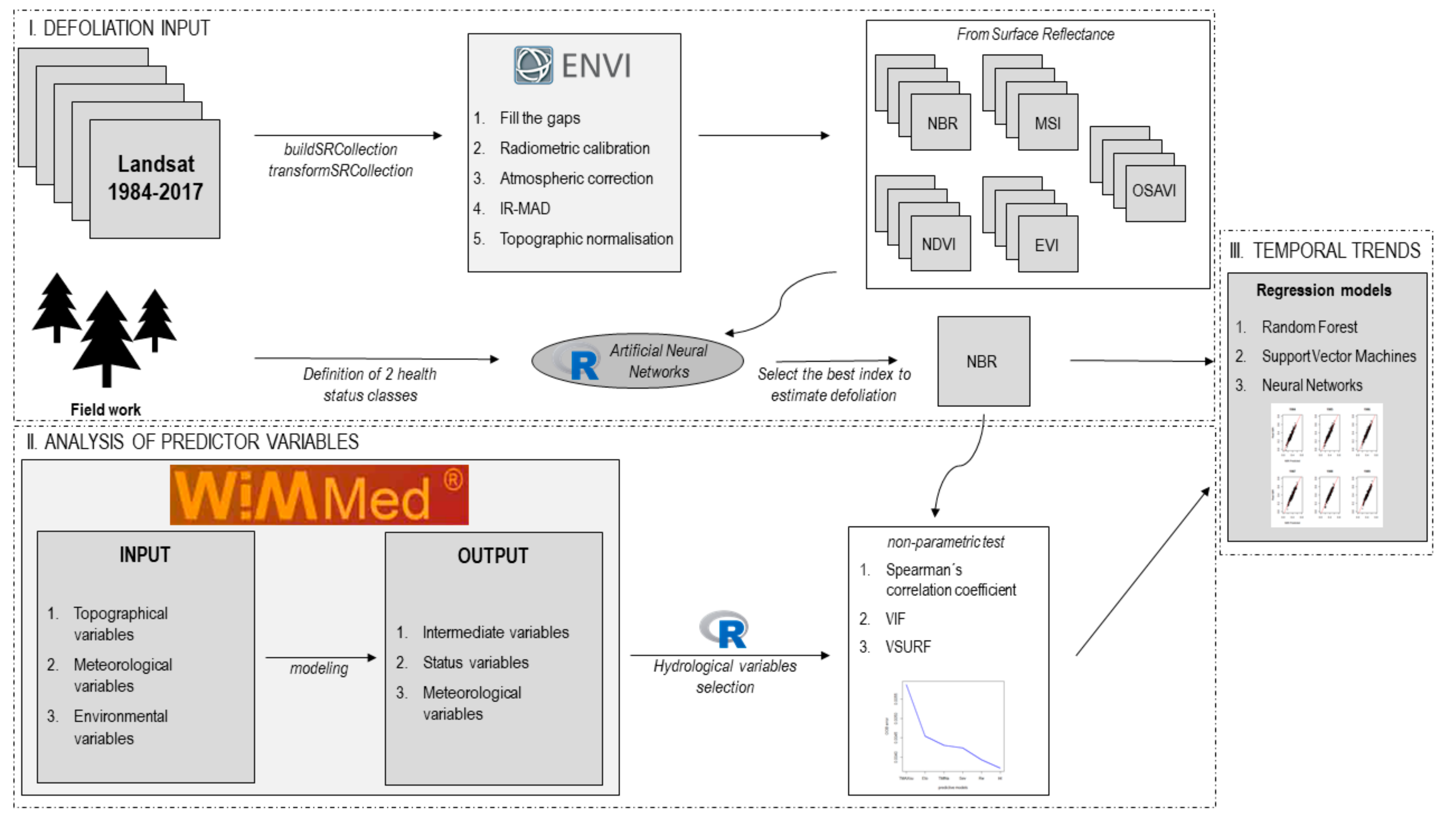
Our study used several data sets and required the development of remote sensing indices and data analysis procedures. Therefore, a flow chart outlining the steps and relationships of each process is provided in Figure 2.
The image datasets acquired for this study consisted of 26 Landsat-5 TM, three Landsat-7 ETM+ and five Landsat-8 OLI images (WRS-2 path 200, row 34), ranging between 1984 and 2017. Only images obtained in the latter part of the hydrological year (July, August and September) were considered. All of these datasets were selected based on the absence of cloud cover; however, when we found multiple cloud-free images for a given year, the image acquired closest to September the 1st was selected. The images were downloaded from the United States Geological Survey (USGS), and had been processed as level 1T (precision and terrain corrected) products. Additional geo-referencing was not necessary. On 31 May 2003, the Landsat Enhanced Thematic Plus (ETM+) Scan Line Corrector (SLC) failed. We applied a two-file methodology to fill the gaps in the 2008 and 2012 Landsat-7 ETM+ images [39].
This multi-temporal image series was used to assess the forest health status in each year; however, other factors can contribute to the variability in multi-temporal spectral responses. The new Landsat-8 OLI is slightly different in its spectral response with respect to the previous Landsat-7 ETM+ and Landsat-5 TM. In several comparative studies (see [19,40]), Landsat-8 OLI had higher values of the near-infrared band for vegetative land-cover types than Landsat-7 TM and Landsat-5 TM [41]. However, part of this difference appears to be systematic, and can be removed by regression equations [42]. For this reason, we applied an “absolute-normalization” approach [43] to normalize each image band-by-band to the reference image.
The reference image (2017) was corrected radiometrically using the radiometric gain and offset values associated with the Landsat OLI image. Next, we applied an atmospheric correction with the MODTRAN4 tool provided by the remote sensing software ENVI. The image corrected for the atmospheric surface reflectance was then used to normalize all other images, using the iteratively re-weighted multivariate alteration detection (IR-MAD) technique [44]. In this method, one atmospherically-absolutely-calibrated image (2017) was selected as the reference to which all others were adjusted, using two separate approaches: The selection of Pseudo-invariant Features (PIFs) and statistical ordination (MAD) [43]. Firstly, the IR-MAD transformation found invariant pixels for a partly-artificial dataset. Secondly, the invariant pixels obtained were used to build linear regression equations, which were used to spectrally align each of the six bands of an image. The quality of the normalized images was evaluated in terms of paired t-tests and F-tests for equal means and variances, respectively. Finally, in order to create a consistent and radiometrically-stable multi-temporal series, a topographic normalization was applied. We chose the C-Correction method. The results obtained by other authors indicate that the C-Correction performed better than other methods of topographic correction [45].
All image processing was performed within the ENVI remote sensing image analysis environment (ITT Visual Information Solutions, version 5.3). Extensions to ENVI for the IR-MAD transformation, radiometric normalization and C-Correction were written by Mort Canty in IDL language [44].
Decline in P. pinaster forests is characterized by a reduction in the leaf area (defoliation), thus the Landsat indices based on the fraction of absorbed photosynthetically-active radiation might be appropriate data choices to assess this process [46]. Therefore, once images were processed, four different Vegetation Indices, which were frequently used for defoliation estimation, including the Moisture Stress Index (MSI), the Normalized Difference Vegetation Index (NDVI), optimized soil adjusted vegetation index (OSAVI), the Normalized Burn Ratio (NBR), and the Enhanced Vegetation Index (EVI), were computed (Table 1).

2.4. Estimating Stand Defoliation from Vegetation Indices

We used artificial neural networks (ANN) to select the best index to estimate defoliation. The neural network has several advantages, including its nonparametric nature, arbitrary decision boundary capability, and easy adaptation to different types of data and input structures, making it a promising technique for land-cover classification [52]. We used the multilayer perceptron. This type of neural network is the most popular for image classification [53]. The accuracy of our classification algorithms was evaluated using a hold-out cross-validation [54]. In this case, we used a random sample of 70% from the training data set (45 plots) and carried out backpropagation repeatedly, alternating with forward passes, and thus the validation was performed by data partitioning using a 30% subset of field plots to validate the model [55]. To test the classification model, we calculated the overall accuracy and global error on the basis of confusion matrices.

2.5. Hydrological Model

The Watershed Integrated Management in Mediterranean Environments (WiMMed) model is a physically-based, distributed hydrological model [14]. The algorithms used by the model were developed, taking into account the absence of accurate climate data for these areas, which is largely due to the rough terrain in Mediterranean mountainous areas [56]. WiMMed was used to obtain a spatial interpolation of the meteorological and soil water variables in the soil vadose zone for 1980–2017 at different temporal scales (Table S1, Supplementary Material). The model included corrections with weight for both rainfall and temperature [56], and topographic corrections for solar radiation. The hydrological model WiMMed was calibrated and validated in previous studies in a mountain region near to the study area [14].

2.6. Relationship Between Defoliation and Hydrological Variables

To assess the relationship between the hydrological variables and forest health status, regression models were constructed. However, due to the relatively small number of field observations (64), we set 255 plots over the P. pinaster stands delimited by its distribution in the study area. The plots were randomly distributed by using the Random points inside polygons tool in QGIS 2.18 (QGIS Development Team, 2018), with a minimum distance between these points of 100 m. After the cleaning of points placed out of forested areas or nearby roads, the total number of plots was 255. The value of the selected VI was used as an indicator of forest defoliation in the regression models. This approach allows an increase in the number of observations, and has been validated in other studies [57]. Both types of variables (response and predictors) were obtained in raster format, at a pixel size of 30 m. All of the raster files have the same number of rows and columns, and are aligned so that they match pixel-by-pixel.
The 255 plots of the different defoliation levels were assigned to build a predictive model among defoliation, expressed as VI, and hydrological variables using the Random Forest (RF) machine-learning algorithm [29]. This method does not require statistical assumptions about the nature of the data; for instance, normality or homoscedasticity.
First, we created a correlation matrix using Spearman’s correlation coefficient (non-parametric test). The variables with a p-value > 0.05 were removed. In the second step, we performed a multicollinearity analysis using the Variance Inflation Factor (VIF). The predictor variables with VIF > 10 [58] were removed. The climatic and hydrological variables were reduced to nine non-collinear variables (see Table S1 Supplementary Material), giving the final dataset by a variable selection procedure based on a random forest (RF) Machine Learning Model [59]. Thus, once the best predictor variables had been selected, we build the regression model using RF. Training data selection is one of the major factors determining the degree to which the regression rules can be generalized [60]. Previous studies show that this factor could be more important for obtaining accurate results than the selection of the regression algorithms [61]. We estimated the accuracy of the RF predictions dividing the data set into two segments: One was used to train the model (70%) and the other to validate it (30%). This procedure consisted of three steps. In the first, the variables were ranked according to a variable importance measure, and the unimportant ones were eliminated. The second aimed to select all variables related to the response for interpretation purposes. The third refined the selection by eliminating redundancy from the set of variables selected in the second step, for prediction purposes [62]. In order to evaluate the stability of the selected regression models and for the result to be statistically valid, hold out cross-validations were performed. Finally, the root-mean-squared error (RMSE), average error (AVE), R-squared (R2), Spearman´s rho (S) and root-mean-squared error of the cross-validation (RMSECV) were calculated to assess the regression performance. We used k-fold cross-validation (k = 20).
We performed all analyses using the R software, version 3.4.0 [63]. The yaImpute, extract and vsurf R packages were used to calculate variable selection and regression with RF and the usdm package was used to perform the collinearity analysis [64]. Predictive models were built using the R caret package [65]. For RF, SVMs and NNs, additional R packages—randomForest [66], kernlab [67] and nnet [68], respectively—were used.

2.7. Temporal Trends

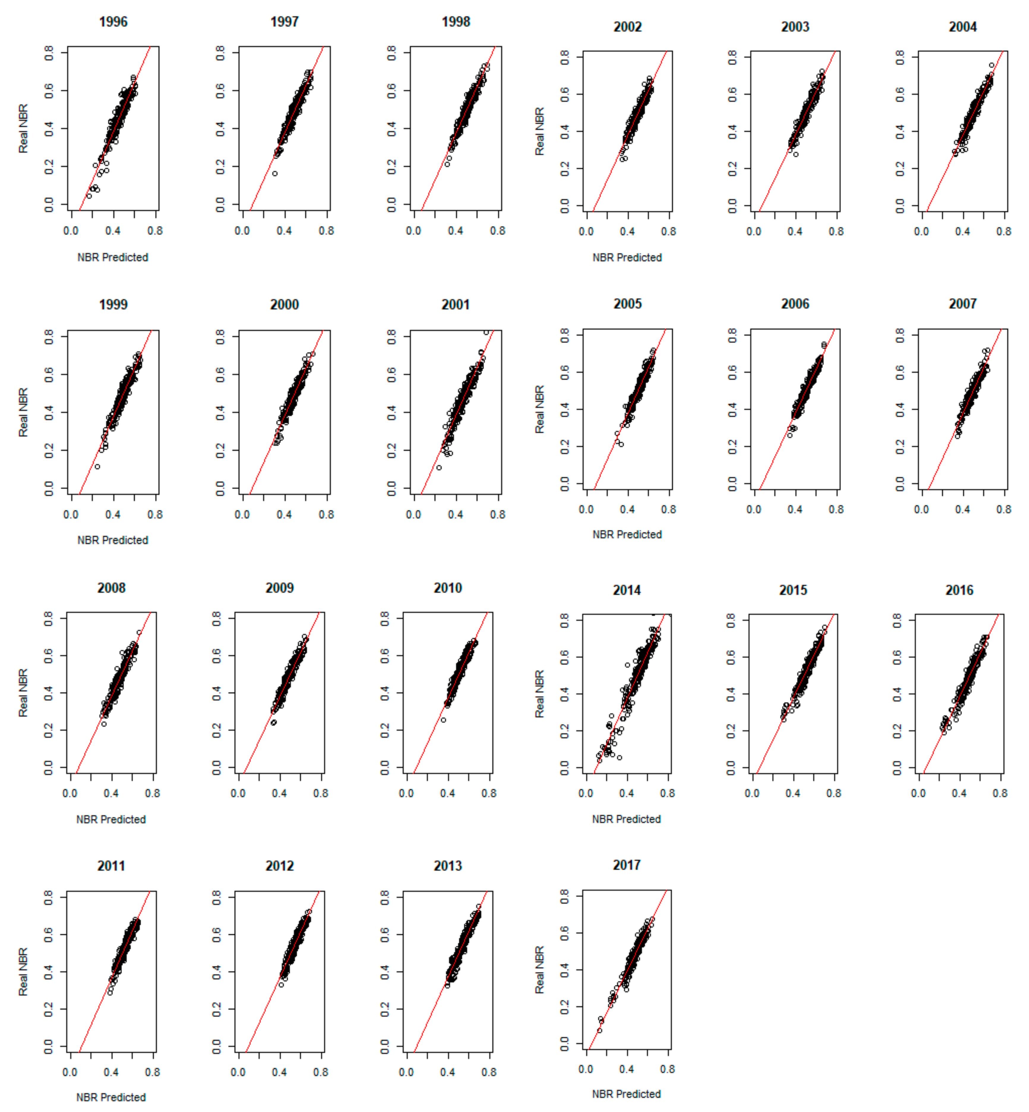
To test the precision of the model along the temporal series, every year was input and tested separately, and the predicted NBR was compared with the real NBR in the same year. Their correlation coefficient and error were calculated. Every statistic result was based upon the 255 sample points.

3. Results

3.1. Estimating Stand Defoliation from Vegetation Indices

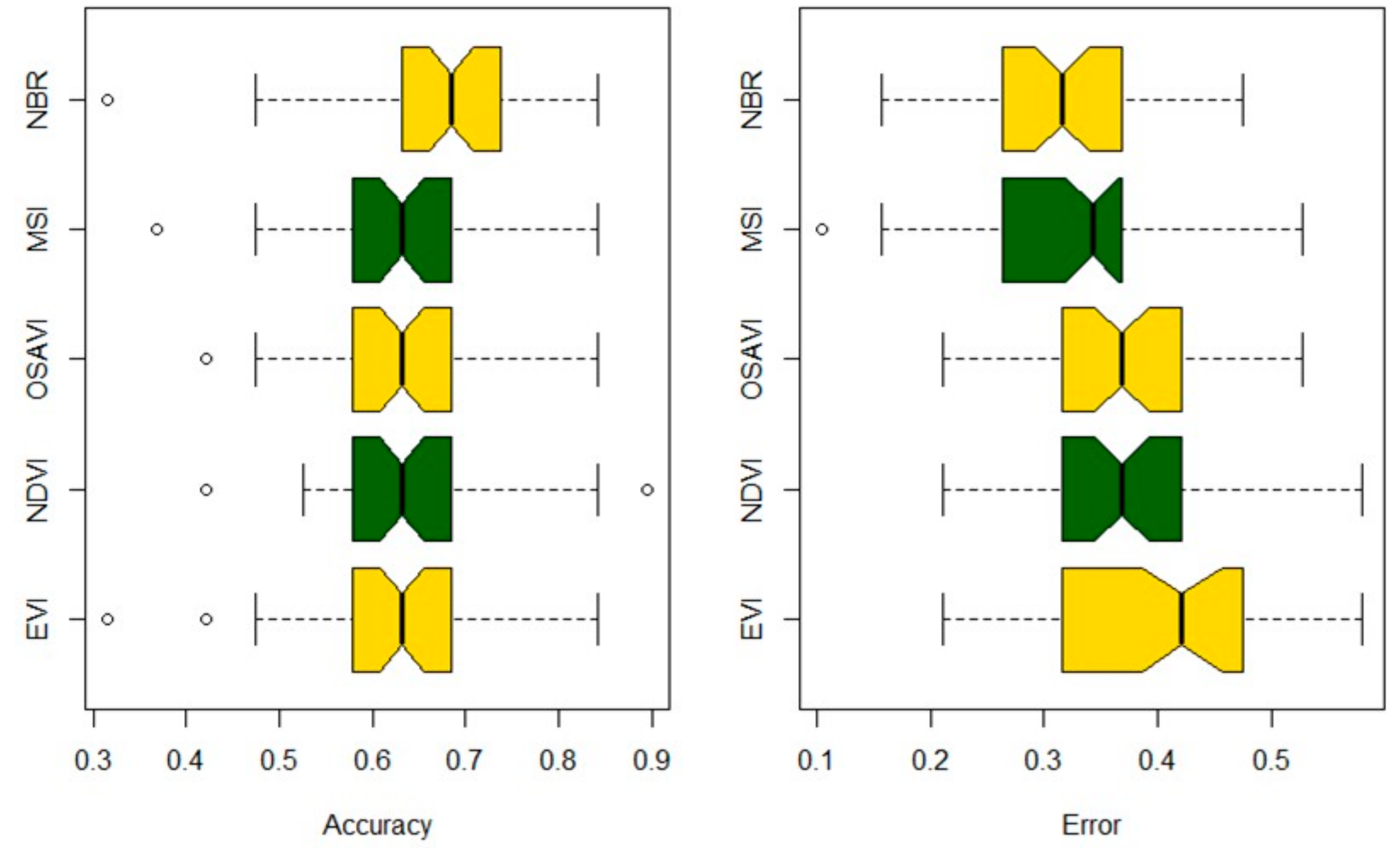
The hold-out cross-validation between the defoliation and VIs is presented in Figure 3. All VIs considered were sensitive to variation in defoliation, nevertheless, the spectral indices that cover different infrared or SWIR areas of the electromagnetic spectrum, showed a strong relationship to defoliation with global accuracy from 0.65 to 0.67 for all of them. The best correlation relationships were observed between the defoliation and MSI and NBR. However, OSAVI, NDVI and EVI showed lower values of accuracy and higher error values. The errors value of NBR was 0.32, slightly better than those of the other VIs, with moderate accuracy prediction results (errors from 0.65 to 0.67), and therefore NBR was used as defoliation input for both model training and temporal trends.

3.2. Relationship between NBR and Hydrological Variables

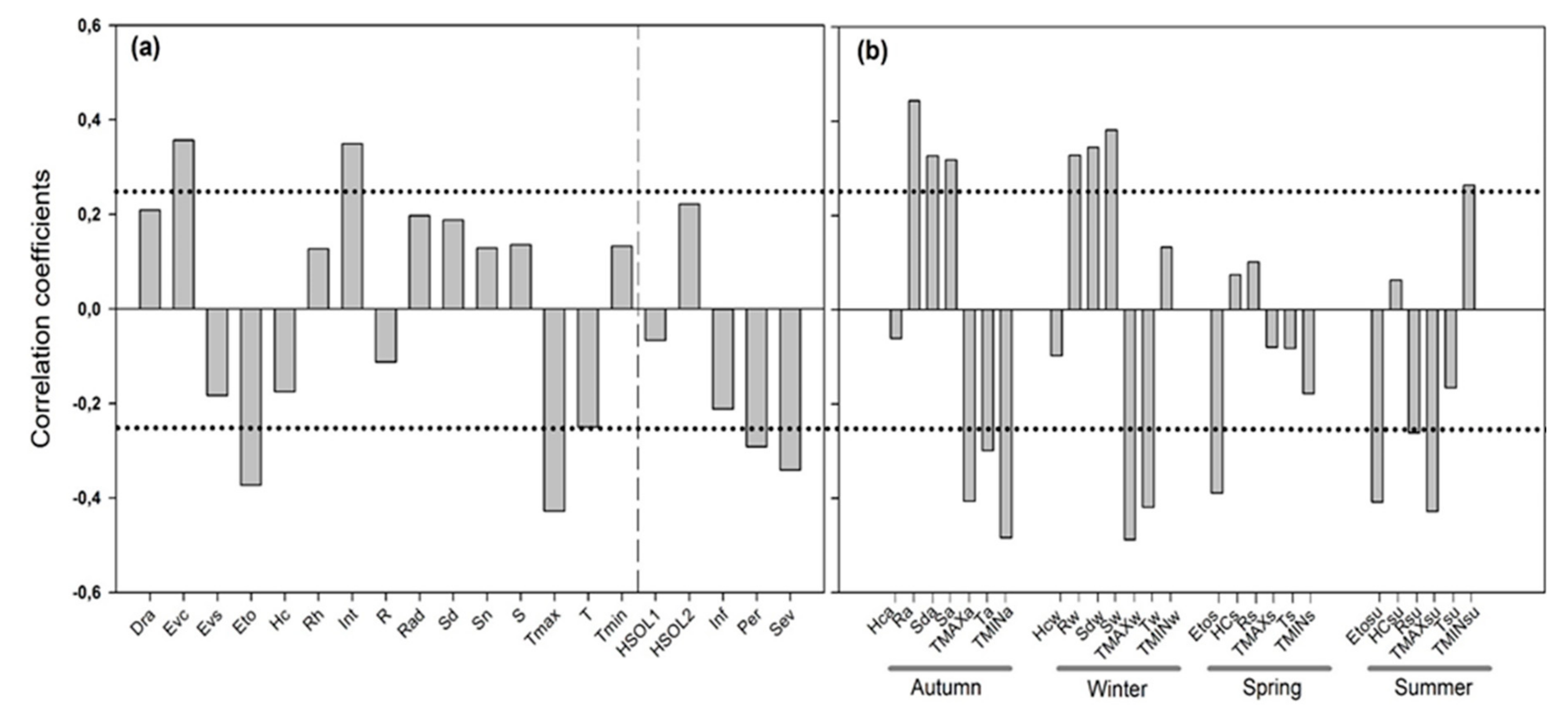
The correlation analysis (Spearman´s test) (Figure 4) revealed a significant relationship between the spatial values of NBR and the hydrological variables. Climate variables at the seasonal scale were better correlated with the NBR index than were the annual variables. Autumn temperatures had significant correlation coefficients (e.g., r = −0.48 with minimum temperature, r = −0.40 with maximum temperature and r = −0.30 with mean temperature). The variables involved in the water balance showed a moderate response to the NBR, with the rainfall as the only variable highly correlated (r = 0.44). Winter temperatures also showed similar correlations (e.g., r = −0.49 with maximum temperature and r = −0.42 with mean temperature). In this season, the value of NBR was significantly related, not only with the variables involved in the water balance, but also with those involved in the snow layer dynamics (r = −0.38 with snowfall and r = 0.34 with snow days). Spring and summer climatic variables showed a similar behavior in the defoliation-climate correlations. In spring the only significant correlation was negatively with the potential evapotranspiration (r = −0.39), and in summer, NBR was negatively correlated to the maximum temperature (r = −0.43) and potential evapotranspiration (r = −0.40). For annual average values, the highest significant correlation coefficients with the NBR were obtained with the maximum temperature (r = −0.43), potential evapotranspiration (r = −0.37), evaporation (r = 0.35), interception (r = 0.34) and soil evaporation (r = −0.34).

3.3. Hydrological Variables Selection

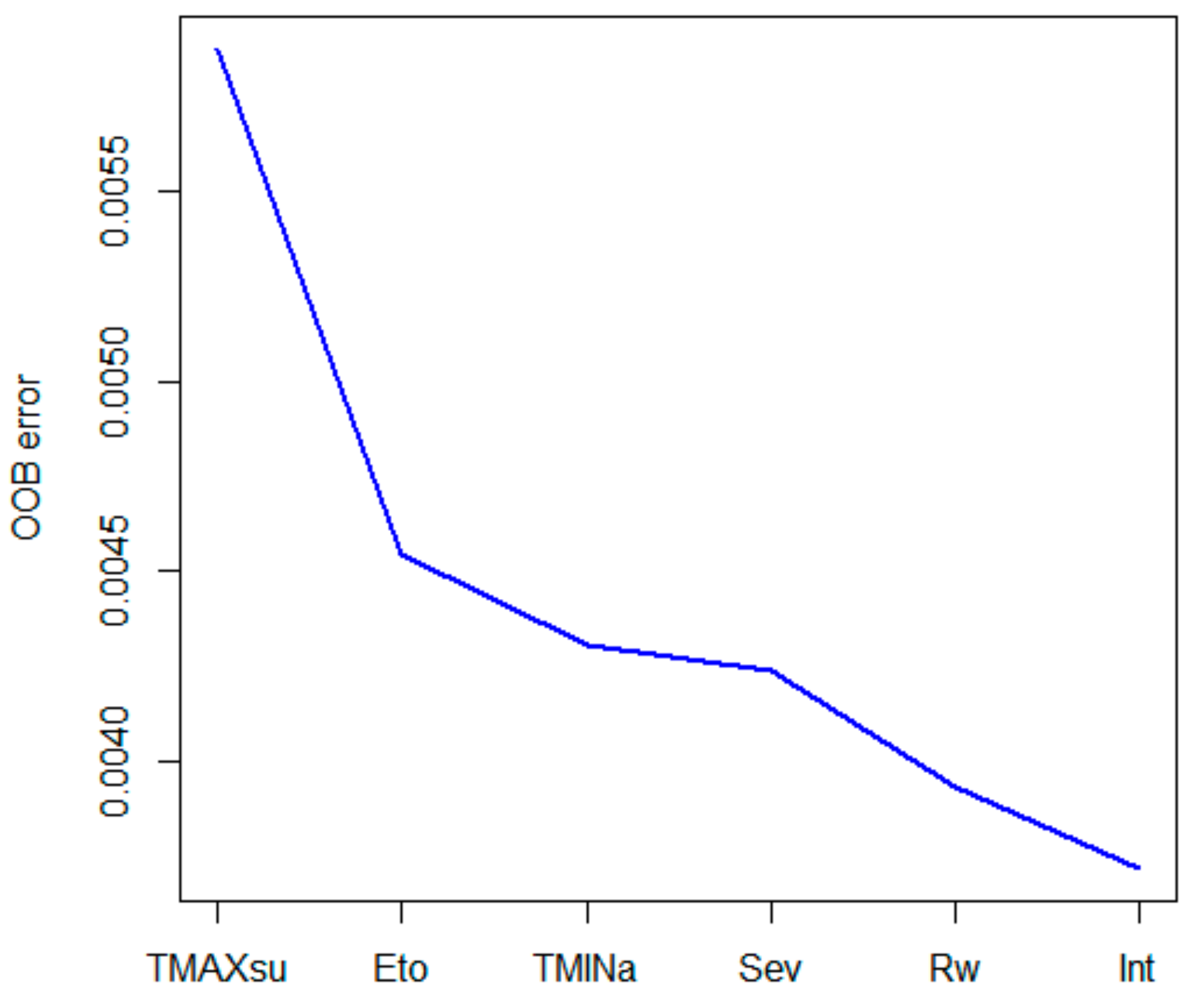
After selecting significant correlations and removing collinear variables, the initial 45 hydrological variables obtained from the WiMMed model were reduced to nine variables by a variable selection procedure based upon RF (VSURF) (Table S1 Supplementary Material). Table S2 (Supplementary Material) contains the relative importance values obtained for each variable, having a higher importance for those related to temperature (maximum temperature, potential evapotranspiration and minimum temperature). The second-highest scores were the variables associated with the soil–water balance (soil evaporation, rainfall and infiltration), while the snow-related variables (e.g., snowfall and number of snow days) had lower values of relative importance (Figure S1 Supplementary Material). The selected variables were those that provided important information and reduced the Out-of-bag (OOB) error (Figure 5), the most-important predictor variables being: Maximum temperature of summer, potential evapotranspiration, minimum temperature of autumn, soil evaporation, rainfall of winter and interception, and three variables were eliminated: (Infiltration, snow days in winter and snowfall in autumn).
Then we used random forest (RF), artificial neural networks (ANN) and support vector machines (SVM) to estimate defoliation (Table 2; Figure 6, Figure S2 Supplementary Material). The defoliation models based on regression methods provided R2 values that ranged from 0.70 to 0.79 (Table 2), with RMSECV and RMSE below 12%. The RF model achieved the highest overall accuracy (R2 = 0.79; RMSECV = 0.05). The SVM and NN models showed similar behavior regarding the performance metrics, with R2 values of 0.70 and 0.71, respectively. The models showed moderate values of S and AVE.

3.4. Temporal Trends

To test the precision of the model, every year of the Landsat temporal series was tested separately. The NBR of the predicted year was calculated by the real NBR in the last year. Then, the predicted NBR was compared with the real NBR in the same year (Figure 6). Every statistic result was based on the 255 sample points. The correlation coefficient between the predicted NBR and the real NBR ranged from 0.84–0.36 (Table S3 Supplementary Material). Of the 34 predicted years, 1994 obtained the best prediction, and there were also some years with a lower correlation coefficient, such as 1996, 1999, 2007 and 2011. This result showed that the NBR model could effectively forecast the defoliation of the damaged P. pinaster trees, and could provide the basis for prediction of the forest defoliation occurrence.

4. Discussion

In the presented study, we investigated the cause-effect relationship between the defoliation of Pinus pinaster forests in southern Spain using vegetation indices derived from Landsat satellite data and hydrological variables at the site scale, obtained with the hydrological model WiMMed, using three machine learning methods: RF, SVM and ANN. This study demonstrates the usefulness of integrating the NBR index derived from Landsat data and hydrological models in the assessment of forest decline-defoliation and environmental drivers, over more conventional remote sensing approaches that only map the defoliation images.

4.1. Vegetation Indexes and Defoliation

Forest decline processes are evident in the spectral properties of sensors which are reflected on vegetation indexes [69]. Visible-near infrared single spectral indices (e.g., NDVI, EVI and OSAVI) have been the most commonly used index for mapping forest defoliation, because they are better related with the chlorophyll content and physiological status of vegetation [70]. Other remote sensing studies of defoliation have found that spectral indices covering different shortwave-infrared or SWIR bands (e.g., NDMI, MSI) are more sensitive to plant water content [71]. More recently, NBR has been proposed to assess forest decline, since those processes are related to chlorosis and structural changes in the canopy caused by tree defoliation and mortality with a spectral behavior similar to forest fires [69,71]. In our case, visible-near infrared spectral indices (NDVI, OSAVI and EVI) performed worse than SWIR bands indices (NBR and MSI). We speculate that visible-near infrared spectral indices were less sensitive to defoliation as a result of saturation effects, and correlate better in more severe defoliation classes [72]. On the contrary, the use of NBR to defoliation assessment is online with previous studies, which also found a robust relationship of canopy defoliation with SWIR data for detecting forest decline processes [71]. It could be explained because defoliated pine forest canopy exposed more soil information on the image, and remaining needles also turned dry, decreasing the total amount of chlorophyll in the canopy leading to strong contrasts in NBR values [73]. Therefore, it is reliable and feasible to apply NBR to assess the forest damage involved with needle canopy changes, both related to simultaneous defoliation and needle mortality.
On this study, only Landsat images acquired at the highest potential defoliation occurrence (end of summer) were used. Considering an image at the end of the more stressful season for Mediterranean forests (summer) can offer a final annual “season-integrated” assessment of defoliation, providing a relatively robust assessment in forest condition over the course of the year. Coniferous decline is often associated with a sudden decrease in one or several spectral indices, different to other gradual processes of coniferous defoliation [74,75]. In fact, there is evidence that coniferous defoliators processes are commonly longer in period than decline processes, with the latter leading to tree mortality within a few years [76]. This suggests that modifications in leaf area are more essential for detecting tree mortality than adjustments in water content or canopy structure.
Another relevant question when studying coniferous defoliation is the use of severity categories (i.e., trace, low, medium, strong defoliation) instead of considering defoliation as a continuous variable based on field data measures [71,77]. On this study, we used a concept of defoliation included in the ICP manual (http://icp-forests.net/page/icp-forests-manual; Part IV), in particular compared to assessing the loss in foliage within one year to estimate the severity of defoliation in terms of canopy changes. Other remote sensing products, as photographic aerial data, have been frequently used as the primary approach for large-scale defoliation assessment [78]. However, visual interpretation is highly subjective and difficult to cover large areas, and does not provide the spatial continuity, multi-temporal assessment and potential for near-real-time and longer-term assessment of annual temporal defoliation processes [79]. Thus, the Landsat defoliation assessment is better to differentiate the magnitude of defoliation and mapping.

4.2. Defoliation and Hydrological Variables

Several studies have identified water availability as the most-important factor in mortality processes in coniferous forests [13]. However, there is a lack of understanding of the long-term interactions between forests status and water balance at the watershed scale. The NBR-defoliation product provides a continuous estimate of defoliator damage at a 30 m spatial resolution covering the whole study area and showing a spatial pattern of defoliation. However, understanding the cause-effect relationship between forest health and hydrological patterns is mandatory to understand the influence of water availability on forest conditions. Thus, we analyzed the correlation between NBR-defoliation and hydrological variables, such as rainfall [80], evapotranspiration [81], temperature [82] and soil moisture [83].
Here, by using the WiMMed hydrological model, we obtained spatially-distributed hydrological variables for the entire study area at a 30 m spatial resolution to examine spatially-explicit relationships between mortality processes and the hydrological regime.
The non-linear approach in defoliation studies has gained heightened research interest in the last decade [27]. Remotely-sensed and ancillary data used in heterogeneous landscapes can be non-normal, multi-model and categorical [84]. For this reason, non-parametric methods have been widely used, especially when a complex interaction among variables exists. Random forest, SVMs and NNs are some of the ML methods most widely used in the context of forests defoliation assessment [32]. In particular, the ability of methods based upon RF to identify ecologically-important predictors has been tested already [85]. On this study, RF developed the most-accurate model (RMSECV = 0.059, R2 = 0.79), showing a high model performance and a very good agreement between the data and predictions, although SVMs and NNs also demonstrated a high performance (R2 > 0.7). These results are in line with the observations of [86] and [87], who also compared different ML approaches in satellite-based land-cover mapping research.
The RF model selected the maximum temperature of summer, potential evapotranspiration, minimum temperature of autumn, soil evaporation, rainfall of winter and interception as the most-important predictors of the defoliation of Maritime pine stands in the study area. This finding is in line with previous studies based on dendrochronological data and the analysis of climate series, showing the impact of climate trends to predispose forests to decline, in particular, a high sensitivity of the growth of defoliated trees to precipitation and maximum temperatures [5,36,88]. This suggests that tree growth decline, and subsequent needle loss, was caused by warming-induced drought stress. Nevertheless, defoliation was not affected solely by the variables involved in the evaporation processes. A positive, linear relationship between NBR and variables involved in the water balance (e.g., rainfall and snowfall) was also observed. A similar significant correlation was obtained in a close area (Guadalfeo watershed-Granada) by [89], who found that the natural vegetative cover was a good indicator of soil moisture conditions. These results confirmed that drought-related defoliation-mortality processes occur more frequently on dry and warm microsites. These were in accordance with the effects of temperature and drought duration, and events in combination with low-water quality sites cause on defoliation-mortality drought processes, and lead to changes in physiological processes related to forest decline [90]. Therefore, the low quality hydrological conditions increased P. pinaster forest mortality in contrast, sites with water compensation balance (e.g., north face and deeper soils) offer “microsites” refuges to some pine stands.

4.3. Temporal Trends

The selection of the reference year for fitting defoliation models is a critical step in Landsat Temporal series analysis process. However, in the study area, defoliation events may have occurred more frequently and more progressively in previous decades, therefore, we cannot assume a 30-year stable base period leading up to our 2017 monitoring period. In other near forests (Pinus sylvestris, P. nigra at Sierra de los Filabres), defoliation processes have been described in previous decades [5,88], although in our location, the defoliation and mortality of P. pinaster and P. halepensis have recently occurred abruptly [34,36]. Because the model is based on a long temporal cycle, information from the time series should improve the ability to fit the models necessary for generating long term assessment. Use of the temporal domain can also be adjusted to generalize our approach to other decline events, including severe outbreaks pests [34]. By targeting condition monitoring at periods associated with specific defoliation causes, it may be possible to study defoliation cycles as observed on this study. We have observed years of severe defoliation associated with drought (1994, [88]), and others with less severe defoliation (e.g., 1996, 1999, 2007 and 2011). The interpretation of temporal defoliation series will need to be dealt with long term environmental and site-defoliators diagnosis and their variation across large areas.
Some restrictions can be considered in this paper. The number of field plots was limited to 65 samples. However, the regressed result of the defoliation ratio by NBR was statistically significant, and it seems not affected by the field plots. Those were selected carefully on pure pine forest with a similar defoliation situation. However, although defoliation on the study region was mainly related to climatic drivers [36], in some locations pest damages and forest management disturbance could have also caused defoliation, and therefore induce some sources of error in the predictions. This can be observed on the better accuracy of the defoliation model in the drought damage years (e.g., 1994, 1998, 2006, 2012 and 2015). Additionally, the effect of pine forests growth over the study period modified VI values [34]. However, the effect of defoliation was considered much greater than pine growth, and the inversion of the defoliation model can be accepted in accordance with other dendrochronological records in the study area [88]. Finally, the hydrological factors were clearly related to the defoliation process, but study is still needed to improve the interpretation of environmental variables into the WiMMed model in order to increase its accuracy. Thus, the integration of the spatiotemporal hydrological prediction model with long time-series prediction could optimize the damage prediction results and make the interpolation of hydrological WiMMed variables more realistic.

4.4. Toward an Integrated Defoliation Monitoring System

Previous studies have suggested that it is possible to estimate defoliation at regional scales using Landsat temporal series [34], offering an operationally monitoring defoliation tool. Therefore, we consider this work as a new relevant contribution to illustrate how dense time series data could be used as part of a near-real-time defoliation monitoring system. Additionally, the Landsat-based disturbance monitoring system has demonstrated to be very useful to be a complementary approach enabling a rapid detection of potential defoliation outbreak events over large spatial extents. Finally, our near-real-time monitoring results can be also used to determine the environmental and hydrological causes behind defoliation outbreaks. This information could be used to inform foresters, concentrating silvicultural efforts on places shown to be impacted at operational scales over large areas. Furthermore, the integration of free remote sensing data (e.g., Sentinel-2) or high resolution satellites (e.g., WorldView-2 sensor) would notably improve the spatial and temporal assessments [28,32].

5. Conclusions

Our findings offer evidence of the effect of the hydrological regime, specifically variables related to the soil–water content, on defoliation processes in Maritime pine plantation in Sierra de Baza (Andalusia-Granada). The Normalized Burn Ratio index (NBR) of Landsat data was strongly proven appropriate to assess and predict the defoliation processes of Pinus pinaster plantations. The patterns of hydrological variables in the study site were simulated through a physically-based, distributed hydrological model (WiMMed). Defoliation was significantly correlated with variables involved in the evaporation processes, such as the maximum temperature of summer (TMAXsu) and potential evapotranspiration (Eto), followed by the minimum temperature of autumn (TMINa), the soil evaporation (Sev), the rainfall of winter (Rw) and the interception (Int). We evaluated the performance of three machine learning methods (random forest, support vector machines and neural networks), concluding that the random forests model was the most stable (R2 = 0.79; RMSECV = 0.05). Finally, temporal trends were assessed for the response variables providing useful information about the extent and direction of their effects. The integration of information derived from hydrological models with temporal series of Landsat images represents a helpful methodology for assessing and predicting the defoliation damage done by complex, environmental, long-term processes that influence drought-triggered mortality. This information provides forest managers with the basis to develop adaptive silvicultural strategies to protect drought-sensitive Mediterranean pine plantations. We presented a set of working hypotheses that will help identify which environmental variables and associated silvicultural systems best meet current and future management goals on these plantations.

Supplementary Materials

The following are available online at https://www.mdpi.com/2072-4292/11/19/2291/s1, Figure S1. Hydrological variables derived from your WiMMed model. Average summer Maximum temperature (TMAXsu), Potential evapotranspiration (Eto), Average annual Minimum temperature (TMINa), Soil evaporation (Sev), Winter rainfall (Rw), Infiltration (Inf), Snowdays in winter (SDw), Annual Snowfall (Sa), Interception (Int), Figure S2. Performance of regression models as a function of training data size used to study the defoliation of Pinus pinaster forests in Sierra de Baza (Andalusia-Granada). (a) Regression model random forest, (b) support vector machines, (c) neural networks, Table S1. Hydrological variables generated from the WiMMed model. In italics, variables obtained from the first and second step of the variable selection procedure (correlation analysis and VIF). In black italic type, chosen variables by VSURF variable selection to build the regression models, Table S2. Relative importance values for hydrological variables according to VSURF variable selection used to assess Maritime pine stands in the decline process in Sierra de Baza (Andalusia-Granada), Table S3. Relative importance values for hydrological variables according to VSURF variable selection used to assess Maritime pine stands in decline process in Sierra de Baza (Andalusia-Granada).

Author Contributions

Conceptualization, R.N. and A.S.; Methodology, A.S., R.N., M.J.P.; Formal Analysis, A.S., R.N. and M.J.P.P.; Investigation, A.S., R.N., and M.J.P.P.; Writing—Original Draft Preparation, R.N. and A.S.; Writing—Review & Editing, R.N., A.S., F.B., M.J.P. and M.J.P.P.

Funding

This research was funded by the Ministerio de Ciencia, Innovación y Universidades (Spain), through the ESPECTRAMED (CGL2017-86161-R), ECOPOTENTIAL (grant agreement No.641762), and ISO-Pine (UCO-1265298) projects.

Acknowledgments

The authors thank the Andalusia Department of Agriculture and Environment, which provided access to and background information on the field site, in particular to the forest health technicians (Red SEDA), JM Ruiz Navarro, MA Gómez de Dios, and A Muñoz Risueño. Also to mention the help provided by “Plan Propio de la UGR” and “Programa de Unidades de Excelencia”, for the publication of this article. We are very grateful to Javier Herrero Latarón, Carlos Rodríguez, Cristina Acosta and Francisco Ruiz-Gómez, for their valuable assistance during fieldwork and data acquisition and processing (without them, this project would not have been possible), and to David Walker, for the linguistic revision of the manuscript. We also acknowledge the institutional support of the University of Cordoba-Campus de Excelencia CEIA3.

Conflicts of Interest

The authors declare no conflict of interest.

References

  1. Barbero, M.; Bonin, G.; Loisel, R.; Quézel, P. Changes and disturbances of forest ecosystems caused by human activities in the western part of the mediterranean basin. Vegetatio 1990, 87, 151–173. [Google Scholar] [CrossRef]
  2. García, J.P.; Goñi, I.I.; Leza, F.J.L. La Restauración forestal de España: 75 años de una ilusión; Ministerio de Agricultura y Pesca, Alimentación y Medio Ambiente: Madrid, Spain, 2017; ISBN 978-84-491-1495-3. [Google Scholar]
  3. Pausas, J.G.; Bladé, C.; Valdecantos, A.; Seva, J.P.; Fuentes, D.; Alloza, J.A.; Vilagrosa, A.; Bautista, S.; Cortina, J.; Vallejo, R. Pines and oaks in the restoration of Mediterranean landscapes of Spain: New perspectives for an old practice—A review. Plant Ecol. 2004, 171, 209–220. [Google Scholar] [CrossRef]
  4. O’Neill, B.C.; Oppenheimer, M.; Warren, R.; Hallegatte, S.; Kopp, R.E.; Pörtner, H.O.; Scholes, R.; Birkmann, J.; Foden, W.; Licker, R.; et al. IPCC reasons for concern regarding climate change risks. Nat. Clim. Chang. 2017, 7, 28–37. [Google Scholar] [CrossRef] [Green Version]
  5. Sánchez-Salguero, R.; Navarro-Cerrillo, R.M.; Camarero, J.J.; Fernández-Cancio, Á. Selective drought-induced decline of pine species in southeastern Spain. Clim. Chang. 2012, 113, 767–785. [Google Scholar] [CrossRef]
  6. Sánchez-Salguero, R.; Camarero, J.J.; Dobbertin, M.; Fernández-Cancio, Á.; Vilà-Cabrera, A.; Manzanedo, R.D.; Zavala, M.A.; Navarro-Cerrillo, R.M. Contrasting vulnerability and resilience to drought-induced decline of densely planted vs. natural rear-edge Pinus nigra forests. For. Ecol. Manag. 2013, 310, 956–967. [Google Scholar] [CrossRef]
  7. Camarero, J.J.; Gazol, A.; Sangüesa-Barreda, G.; Oliva, J.; Vicente-Serrano, S.M. To die or not to die: Early warnings of tree dieback in response to a severe drought. J. Ecol. 2015, 103, 44–57. [Google Scholar] [CrossRef]
  8. Allen, C.D.; Macalady, A.K.; Chenchouni, H.; Bachelet, D.; McDowell, N.; Vennetier, M.; Kitzberger, T.; Rigling, A.; Breshears, D.D.; Hogg, E.H.; et al. A global overview of drought and heat-induced tree mortality reveals emerging climate change risks for forests. For. Ecol. Manag. 2010, 259, 660–684. [Google Scholar] [CrossRef] [Green Version]
  9. Choat, B.; Brodribb, T.J.; Brodersen, C.R.; Duursma, R.A.; López, R.; Medlyn, B.E. Triggers of tree mortality under drought. Nature 2018, 558, 531–539. [Google Scholar] [CrossRef]
  10. Adams, H.D.; Zeppel, M.J.B.; Anderegg, W.R.L.; Hartmann, H.; Landhäusser, S.M.; Tissue, D.T.; Huxman, T.E.; Hudson, P.J.; Franz, T.E.; Allen, C.D.; et al. A multi-species synthesis of physiological mechanisms in drought-induced tree mortality. Nat. Ecol. Evol. 2017, 1, 1285–1291. [Google Scholar] [CrossRef]
  11. Yang, J.; Weisberg, P.J.; Bristow, N.A. Landsat remote sensing approaches for monitoring long-term tree cover dynamics in semi-arid woodlands: Comparison of vegetation indices and spectral mixture analysis. Remote Sens. Environ. 2012, 119, 62–71. [Google Scholar] [CrossRef]
  12. Caldwell, P.V.; Kennen, J.G.; Sun, G.; Kiang, J.E.; Butcher, J.B.; Eddy, M.C.; Hay, L.E.; LaFontaine, J.H.; Hain, E.F.; Nelson, S.A.C.; et al. A comparison of hydrologic models for ecological flows and water availability. Ecohydrology 2015, 8, 1525–1546. [Google Scholar] [CrossRef]
  13. Anderegg, W.R.L.; Martinez-Vilalta, J.; Cailleret, M.; Camarero, J.J.; Ewers, B.E.; Galbraith, D.; Gessler, A.; Grote, R.; Huang, C.; Levick, S.R.; et al. When a Tree Dies in the Forest: Scaling Climate-Driven Tree Mortality to Ecosystem Water and Carbon Fluxes. Ecosystems 2016, 19, 1133–1147. [Google Scholar] [CrossRef] [Green Version]
  14. Polo, M.J.; Herrero, J.; Aguilar, C.; Millares, A.; Monino, A.; Nieto, S.; Losada, M. WiMMed, a Distributed Physically-Based Watershed Model (I): Description and Validation: Environmental Hydraulics: Theoretical, Experimental & Computational Solutions; CRC Press/Balkema: Boca Raton, FL, USA, 2009; pp. 225–228. [Google Scholar]
  15. Anderegg, W.R.L.; Hicke, J.A.; Fisher, R.A.; Allen, C.D.; Aukema, J.; Bentz, B.; Hood, S.; Lichstein, J.W.; Macalady, A.K.; McDowell, N.; et al. Tree mortality from drought, insects, and their interactions in a changing climate. New Phytol. 2015, 208, 674–683. [Google Scholar] [CrossRef] [PubMed]
  16. Hernández-Clemente, R.; Hornero, A.; Mottus, M.; Penuelas, J.; González-Dugo, V.; Jiménez, J.C.; Suárez, L.; Alonso, L.; Zarco-Tejada, P.J. Early Diagnosis of Vegetation Health from High-Resolution Hyperspectral and Thermal Imagery: Lessons Learned from Empirical Relationships and Radiative Transfer Modelling. Curr. For. Rep. 2019, 5, 169–183. [Google Scholar] [CrossRef]
  17. Hall, R.J.; van der Sanden, J.J.; Freeburn, J.T.; Thomas, S.J. Remote Sensing of Natural Disturbance Caused by Insect Defoliation and Dieback: A Review; Open File 25; Natural Resources Canada, Geomatics Canada: Edmonton, AB, Canada, 2016. [Google Scholar] [CrossRef]
  18. Banskota, A.; Kayastha, N.; Falkowski, M.J.; Wulder, M.A.; Froese, R.E.; White, J.C. Forest Monitoring Using Landsat Time Series Data: A Review. Can. J. Remote Sens. 2014, 40, 362–384. [Google Scholar] [CrossRef]
  19. Vogelmann, J.E.; Gallant, A.L.; Shi, H.; Zhu, Z. Perspectives on monitoring gradual change across the continuity of Landsat sensors using time-series data. Remote Sens. Environ. 2016, 185, 258–270. [Google Scholar] [CrossRef] [Green Version]
  20. Brodrick, P.G.; Asner, G.P. Remotely sensed predictors of conifer tree mortality during severe drought. Environ. Res. Lett. 2017, 12, 115013. [Google Scholar] [CrossRef] [Green Version]
  21. Navarro-Cerrillo, R.M.; Trujillo, J.; de la Orden, M.S.; Hernández-Clemente, R. Hyperspectral and multispectral satellite sensors for mapping chlorophyll content in a Mediterranean Pinus sylvestris L. plantation. Int. J. Appl. Earth Obs. Geoinf. 2014, 26, 88–96. [Google Scholar] [CrossRef]
  22. Zarco-Tejada, P.J.; Hornero, A.; Beck, P.S.A.; Kattenborn, T.; Kempeneers, P.; Hernández-Clemente, R. Chlorophyll content estimation in an open-canopy conifer forest with Sentinel-2A and hyperspectral imagery in the context of forest decline. Remote Sens. Environ. 2019, 223, 320–335. [Google Scholar] [CrossRef]
  23. Zhu, C.; Zhang, X.; Zhang, N.; Hassan, M.A.; Zhao, L. Assessing the Defoliation of Pine Forests in a Long Time-Series and Spatiotemporal Prediction of the Defoliation Using Landsat Data. Remote Sens. 2018, 10, 360. [Google Scholar] [CrossRef]
  24. Mather, P.; Tso, B. Classification Methods for Remotely Sensed Data; CRC Press, Taylor & Francis Group: Boca Raton, FL, USA, 2016. [Google Scholar]
  25. Kamavisdar, P.; Saluja, S.; Agrawal, S. A Survey on Image Classification Approaches and Techniques. Int. J. Adv. Res. Comput. Commun. Eng. 2013, 2, 5. [Google Scholar]
  26. Adelabu, S.; Dube, T. Employing ground and satellite-based QuickBird data and random forest to discriminate five tree species in a Southern African Woodland. Geocarto Int. 2015, 30, 457–471. [Google Scholar] [CrossRef]
  27. Anees, A.; Aryal, J.; O’Reilly, M.M.; Gale, T.J.; Wardlaw, T. A robust multi-kernel change detection framework for detecting leaf beetle defoliation using Landsat 7 ETM+ data. ISPRS J. Photogramm. Remote Sens. 2016, 122, 167–178. [Google Scholar] [CrossRef]
  28. Lottering, R.; Mutanga, O.; Peerbhay, K.; Ismail, R. Detecting and mapping Gonipterus scutellatus induced vegetation defoliation using WorldView-2 pan-sharpened image texture combinations and an artificial neural network. J. Appl. Remote Sens. 2019, 13, 014513. [Google Scholar] [CrossRef]
  29. Lary, D.J.; Alavi, A.H.; Gandomi, A.H.; Walker, A.L. Machine learning in geosciences and remote sensing. Geosci. Front. 2016, 7, 3–10. [Google Scholar] [CrossRef] [Green Version]
  30. Belgiu, M.; Drăguţ, L. Random forest in remote sensing: A review of applications and future directions. ISPRS J. Photogramm. Remote Sens. 2016, 114, 24–31. [Google Scholar] [CrossRef]
  31. Heydari, S.S.; Mountrakis, G. Effect of classifier selection, reference sample size, reference class distribution and scene heterogeneity in per-pixel classification accuracy using 26 Landsat sites. Remote Sens. Environ. 2018, 204, 648–658. [Google Scholar] [CrossRef]
  32. Hawryło, P.; Bednarz, B.; Wężyk, P.; Szostak, M. Estimating Defoliation of Scots Pine Stands Using Machine Learning Methods and Vegetation Indices of Sentinel-2. Eur. J. Remote Sens. 2017, 51, 194–204. Available online: https://www.tandfonline.com/doi/full/10.1080/22797254.2017.1417745 (accessed on 23 September 2019). [CrossRef]
  33. Tai, X.; Mackay, D.S.; Sperry, J.S.; Brooks, P.; Anderegg, W.R.L.; Flanagan, L.B.; Rood, S.B.; Hopkinson, C. Distributed Plant Hydraulic and Hydrological Modeling to Understand the Susceptibility of Riparian Woodland Trees to Drought-Induced Mortality. Water Resour. Res. 2018, 54, 4901–4915. [Google Scholar] [CrossRef]
  34. Trujillo-Toro, J.; Navarro-Cerrillo, R.M. Analysis of Site-dependent Pinus halepensis Mill. Defoliation Caused by ‘Candidatus Phytoplasma pini’ through Shape Selection in Landsat Time Series. Remote Sens. 2019, 11, 1868. [Google Scholar] [CrossRef]
  35. Fernández-Cancio, A.; Navarro-Cerrillo, R.M.; Sánchez-Salguero, R.; Fernández, R.F.; Menéndez, E.M. Viabilidad fitoclimática de las repoblaciones de pino silvestre (Pinus sylvestris L.) en la Sierra de los Filabres (Almería). Revista Ecosistemas 2011, 20, 124–144. [Google Scholar]
  36. Navarro-Cerrillo, R.M.; Rodriguez-Vallejo, C.; Silveiro, E.; Hortal, A.; Palacios-Rodríguez, G.; Duque-Lazo, J.; Camarero, J.J. Cumulative Drought Stress Leads to a Loss of Growth Resilience and Explains Higher Mortality in Planted than in Naturally Regenerated Pinus pinaster Stands. Forests 2018, 9, 358. [Google Scholar] [CrossRef]
  37. Ferreti, M. (Ed.) 1994: Especies forestales mediterrá—Google Académico. Available online: https://scholar.google.es/scholar?hl=es&as_sdt=0%2C5&q=FERRETI+M.+%28Editor%29%2C+1994%3A+Especies+forestales+mediterr%C3%A1neas.+Gu%C3%ADa+para+la+evaluaci%C3%B3n+de+las+copas.+CEE%C2%ADUN%2FECE.+Bruselas+Ginebra.&btnG= (accessed on 23 August 2019).
  38. Corcuera, L.; Gil-Pelegrín, E.; Notivol, E. Differences in hydraulic architecture between mesic and xeric Pinus pinaster populations at the seedling stage. Tree Physiol. 2012, 32, 1442–1457. [Google Scholar] [CrossRef] [PubMed] [Green Version]
  39. Scaramuzza, P.; Micijevic, E.; Chander, G. SLC previous termGapnext term-filled Products Phase One Methodology, 5. 2004. Available online: http://landsat.usgs.gov/documents/SLC_Gap_Fill_Methodology.pdf. (accessed on 20 July 2019).
  40. Mishra, N.; Helder, D.; Barsi, J.; Markham, B. Continuous calibration improvement in solar reflective bands: Landsat 5 through Landsat 8. Remote Sens. Environ. 2016, 185, 7–15. [Google Scholar] [CrossRef] [PubMed] [Green Version]
  41. Li, P.; Jiang, L.; Feng, Z. Cross-Comparison of Vegetation Indices Derived from Landsat-7 Enhanced Thematic Mapper Plus (ETM+) and Landsat-8 Operational Land Imager (OLI) Sensors. Remote Sens. 2014, 6, 310–329. [Google Scholar] [CrossRef]
  42. Flood, N. Continuity of Reflectance Data between Landsat-7 ETM+ and Landsat-8 OLI, for Both Top-of-Atmosphere and Surface Reflectance: A Study in the Australian Landscape. Remote Sens. 2014, 6, 7952–7970. [Google Scholar] [CrossRef] [Green Version]
  43. Schroeder, T.A.; Cohen, W.B.; Song, C.; Canty, M.J.; Yang, Z. Radiometric correction of multi-temporal Landsat data for characterization of early successional forest patterns in western Oregon. Remote Sens. Environ. 2006, 103, 16–26. [Google Scholar] [CrossRef]
  44. Canty, M.J.; Nielsen, A.A.; Schmidt, M. Automatic radiometric normalization of multitemporal satellite imagery. Remote Sens. Environ. 2004, 91, 441–451. [Google Scholar] [CrossRef] [Green Version]
  45. Hantson, S.; Chuvieco, E. Evaluation of different topographic correction methods for Landsat imagery. Int. J. Appl. Earth Obs. Geoinf. 2011, 13, 691–700. [Google Scholar] [CrossRef]
  46. Silva, C.R.; Olthoff, A.E.; de la Mata, J.A.D.; Alonso, A.P. Remote monitoring of forest insect defoliation. A review. For. Syst. 2013, 22, 377–391. [Google Scholar]
  47. Ramachandran, B.; Justice, C.O.; Abrams, M.J. Land Remote Sensing and Global Environmental Change: NASA’s Earth Observing System and the Science of ASTER and MODIS; Springer Science & Business Media: New York, NY, USA, 2010; ISBN 978-1-4419-6749-7. [Google Scholar]
  48. Hunt, E.R.; Rock, B.N. Detection of changes in leaf water content using Near- and Middle-Infrared reflectances. Remote Sens. Environ. 1989, 30, 43–54. [Google Scholar]
  49. Key, C.H.; Benson, N.; Ohlen, D.; Howard, S.; McKinley, R.; Zhu, Z. The Normalized Burn Ratio and Relationships to Burn Severity: Ecology, Remote Sensing and Implementation. Available online: https://www.indexdatabase.de/db/r-single.php?id=62 (accessed on 23 August 2019).
  50. Rouse, W.; Haas, R.H.; Schell, J.A.; Deering, D.W. In Monitoring vegetation systems in the Great Plains with ERTS; Third ERTS Symposium. NASA SP-351: Washington, DC, USA, 1974; pp. 309–317. [Google Scholar]
  51. Rondeaux, G.; Steven, M.; Baret, F. Optimization of soil-adjusted vegetation indices. Remote Sens. Environ. 1996, 55, 95–107. [Google Scholar] [CrossRef]
  52. Paola, J.D.; Schowengerdt, R.A. A review and analysis of backpropagation neural networks for classification of remotely-sensed multi-spectral imagery. Int. J. Remote Sens. 1995, 16, 3033–3058. [Google Scholar] [CrossRef]
  53. Atkinson, P.M.; Tatnall, A.R.L. Introduction Neural networks in remote sensing. Int. J. Remote Sens. 1997, 18, 699–709. [Google Scholar] [CrossRef]
  54. Chen, L.-C.; Papandreou, G.; Kokkinos, I.; Murphy, K.; Yuille, A.L. Semantic Image Segmentation with Deep Convolutional Nets and Fully Connected CRFs. arXiv 2014, arXiv:14127062. [Google Scholar]
  55. Jung, Y.; Hu, J. A K-fold averaging cross-validation procedure. J. Nonparametr. Stat. 2015, 27, 167–179. [Google Scholar] [CrossRef] [PubMed]
  56. Herrero, J.; Aguilar, C.; Polo, M.J.; Losada, M. Mapping of meteorological variables for runoff generation forecast in distributed hydrological modeling. In Proceedings of the Hydraulic Measurements & Experimental Methods 2007, Lake Placid, NY, USA, 10–12 September 2007. [Google Scholar]
  57. Porcar-Castell, A.; Tyystjärvi, E.; Atherton, J.; van der Tol, C.; Flexas, J.; Pfündel, E.E.; Moreno, J.; Frankenberg, C.; Berry, J.A. Linking chlorophyll a fluorescence to photosynthesis for remote sensing applications: Mechanisms and challenges. J. Exp. Bot. 2014, 65, 4065–4095. [Google Scholar] [CrossRef]
  58. Duque-Lazo, J.; Navarro-Cerrillo, R.M. What to save, the host or the pest? The spatial distribution of xylophage insects within the Mediterranean oak woodlands of Southwestern Spain. For. Ecol. Manag. 2017, 392, 90–104. [Google Scholar] [CrossRef]
  59. Breiman, L. Random Forests. Mach. Learn. 2001, 45, 5–32. [Google Scholar] [CrossRef] [Green Version]
  60. Paola, J.D.; Schowengerdt, R.A. A detailed comparison of backpropagation neural network and maximum-likelihood classifiers for urban land use classification. IEEE Trans. Geosci. Remote Sens. 1995, 33, 981–996. [Google Scholar] [CrossRef]
  61. Huang, G.-B.; Ding, X.; Zhou, H. Optimization method based extreme learning machine for classification. Neurocomputing 2010, 74, 155–163. [Google Scholar] [CrossRef]
  62. Genuer, R.; Poggi, J.-M.; Tuleau-Malot, C. VSURF: An R Package for Variable Selection Using Random Forests. R J. 2015, 7, 19–33. [Google Scholar] [CrossRef] [Green Version]
  63. Liaw, A.; Wiener, M. Classifcation and Regression by randomForest (R news). 2002. Available online: https://www.r-project.org/doc/ Rnews/Rnews_2002-3.pdf (accessed on 10 May 2019).
  64. Crookston, N.L.; Finley, A.O. yaImpute: An R package for kNN imputation. J. Stat. Softw. 2008, 23. [Google Scholar] [CrossRef]
  65. Kuhn, M. Building Predictive Models in R Using the caret Package. J. Stat. Softw. 2008, 28. [Google Scholar] [CrossRef]
  66. Liaw, A.; Wiener, M. The randomforest package. R News 2002, 2, 18–22. [Google Scholar]
  67. Hornik, K.; Meyer, D.; Karatzoglou, A. Support Vector Machines in R. J. Stat. Softw. 2006, 15, 1–28. [Google Scholar]
  68. Ripley B nnet: Feed-Forward Neural Networks and Multinomial Log-Linear Models. R package version 7.3-9, 2015. Available online: http://CRAN.R-project.org/package=nnet.
  69. Senf, C.; Pflugmacher, D.; Wulder, M.A.; Hostert, P. Characterizing spectral–temporal patterns of defoliator and bark beetle disturbances using Landsat time series. Remote Sens. Environ. 2015, 170, 166–177. [Google Scholar] [CrossRef]
  70. Xue, J.; Su, B. Significant Remote Sensing Vegetation Indices: A Review of Developments and Applications. Available online: https://www.hindawi.com/journals/js/2017/1353691/abs/ (accessed on 23 August 2019).
  71. Townsend, P.A.; Singh, A.; Foster, J.R.; Rehberg, N.J.; Kingdon, C.C.; Eshleman, K.N.; Seagle, S.W. A general Landsat model to predict canopy defoliation in broadleaf deciduous forests. Remote Sens. Environ. 2012, 119, 255–265. [Google Scholar] [CrossRef]
  72. Marx, A.; Kleinschmit, B. Sensitivity analysis of RapidEye spectral bands and derived vegetation indices for insect defoliation detection in pure Scots pine stands. IForest Biogeosci. For. 2017, 10, 659. [Google Scholar] [CrossRef]
  73. Szporak-Wasilewska, S.; Krettek, O.; Berezowski, T.; Ejdys, B.; Sławik, Ł.; Borowski, M.; Chormański, J. Leaf area index of forests using ALS, Landsat and ground measurements in Magura National Park (SE Poland). EARSeL eProc. 2014, 13, 103–111. [Google Scholar]
  74. Vogelmann, J.E.; Tolk, B.; Zhu, Z. Monitoring forest changes in the southwestern United States using multitemporal Landsat data. Remote Sens. Environ. 2009, 113, 1739–1748. [Google Scholar] [CrossRef]
  75. Meigs, G.W.; Kennedy, R.E.; Cohen, W.B. A Landsat time series approach to characterize bark beetle and defoliator impacts on tree mortality and surface fuels in conifer forests. Remote Sens. Environ. 2011, 115, 3707–3718. [Google Scholar] [CrossRef]
  76. Neumann, M.; Mues, V.; Moreno, A.; Hasenauer, H.; Seidl, R. Climate variability drives recent tree mortality in Europe. Glob. Chang. Biol. 2017, 23, 4788–4797. [Google Scholar] [CrossRef] [PubMed]
  77. Rullán-Silva, C.; Olthoff, A.E.; Pando, V.; Pajares, J.A.; Delgado, J.A. Remote monitoring of defoliation by the beech leaf-mining weevil Rhynchaenus fagi in northern Spain. For. Ecol. Manag. 2015, 347, 200–208. [Google Scholar] [CrossRef]
  78. Goodbody, T.R.H.; Coops, N.C.; Hermosilla, T.; Tompalski, P.; McCartney, G.; MacLean, D.A. Digital aerial photogrammetry for assessing cumulative spruce budworm defoliation and enhancing forest inventories at a landscape-level. ISPRS J. Photogramm. Remote Sens. 2018, 142, 1–11. [Google Scholar] [CrossRef]
  79. Johnson, E.W.; Ross, J. Quantifying error in aerial survey data. Aust. For. 2008, 71, 216–222. [Google Scholar] [CrossRef]
  80. Ji, L.; Peters, A.J. Assessing vegetation response to drought in the northern Great Plains using vegetation and drought indices. Remote Sens. Environ. 2003, 87, 85–98. [Google Scholar] [CrossRef]
  81. Groeneveld, D.P. Remotely-sensed groundwater evapotranspiration from alkali scrub affected by declining water table. J. Hydrol. 2008, 358, 294–303. [Google Scholar] [CrossRef]
  82. Wang, J.; Rich, P.M.; Price, K.P. Temporal responses of NDVI to precipitation and temperature in the central Great Plains, USA. Int. J. Remote Sens. 2003, 24, 2345–2364. [Google Scholar] [CrossRef]
  83. Adegoke, J.O.; Carleton, A.M. Relations between Soil Moisture and Satellite Vegetation Indices in the U.S. Corn Belt. J. Hydrometeorol. 2002, 3, 395–405. [Google Scholar] [CrossRef] [Green Version]
  84. Ghimire, B.; Rogan, J.; Galiano, V.R.; Panday, P.; Neeti, N. An Evaluation of Bagging, Boosting, and Random Forests for Land-Cover Classification in Cape Cod, Massachusetts, USA. GISci. Remote Sens. 2012, 49, 623–643. [Google Scholar] [CrossRef]
  85. Vitale, M.; Proietti, C.; Cionni, I.; Fischer, R.; De Marco, A. Random Forests Analysis: A Useful Tool for Defining the Relative Importance of Environmental Conditions on Crown Defoliation. Water Air Soil Pollut. 2014, 225, 1992. [Google Scholar] [CrossRef]
  86. Yu, L.; Liang, L.; Wang, J.; Zhao, Y.; Cheng, Q.; Hu, L.; Liu, S.; Yu, L.; Wang, X.; Zhu, P.; et al. Meta-discoveries from a synthesis of satellite-based land-cover mapping research. Int. J. Remote Sens. 2014, 35, 4573–4588. [Google Scholar] [CrossRef]
  87. Lu, D.; Weng, Q. A survey of image classification methods and techniques for improving classification performance. Int. J. Remote Sens. 2007, 28, 823–870. [Google Scholar] [CrossRef]
  88. Sánchez-Salguero, R.; Navarro, R.M.; Camarero, J.J.; Fernández-Cancio, Á. Drought-induced growth decline of Aleppo and maritime pine forests in south-eastern Spain. For. Syst. 2010, 19, 458–470. [Google Scholar] [CrossRef]
  89. Gómez-Giráldez, P.J.; Aguilar, C.; Polo, M.J. Natural vegetation covers as indicators of the soil water content in a semiarid mountainous watershed. Ecol. Indic. 2014, 46, 524–535. [Google Scholar] [CrossRef]
  90. Klein, T. Drought-induced tree mortality: From discrete observations to comprehensive research. Tree Physiol. 2015, 35, 225–228. [Google Scholar] [CrossRef] [PubMed]
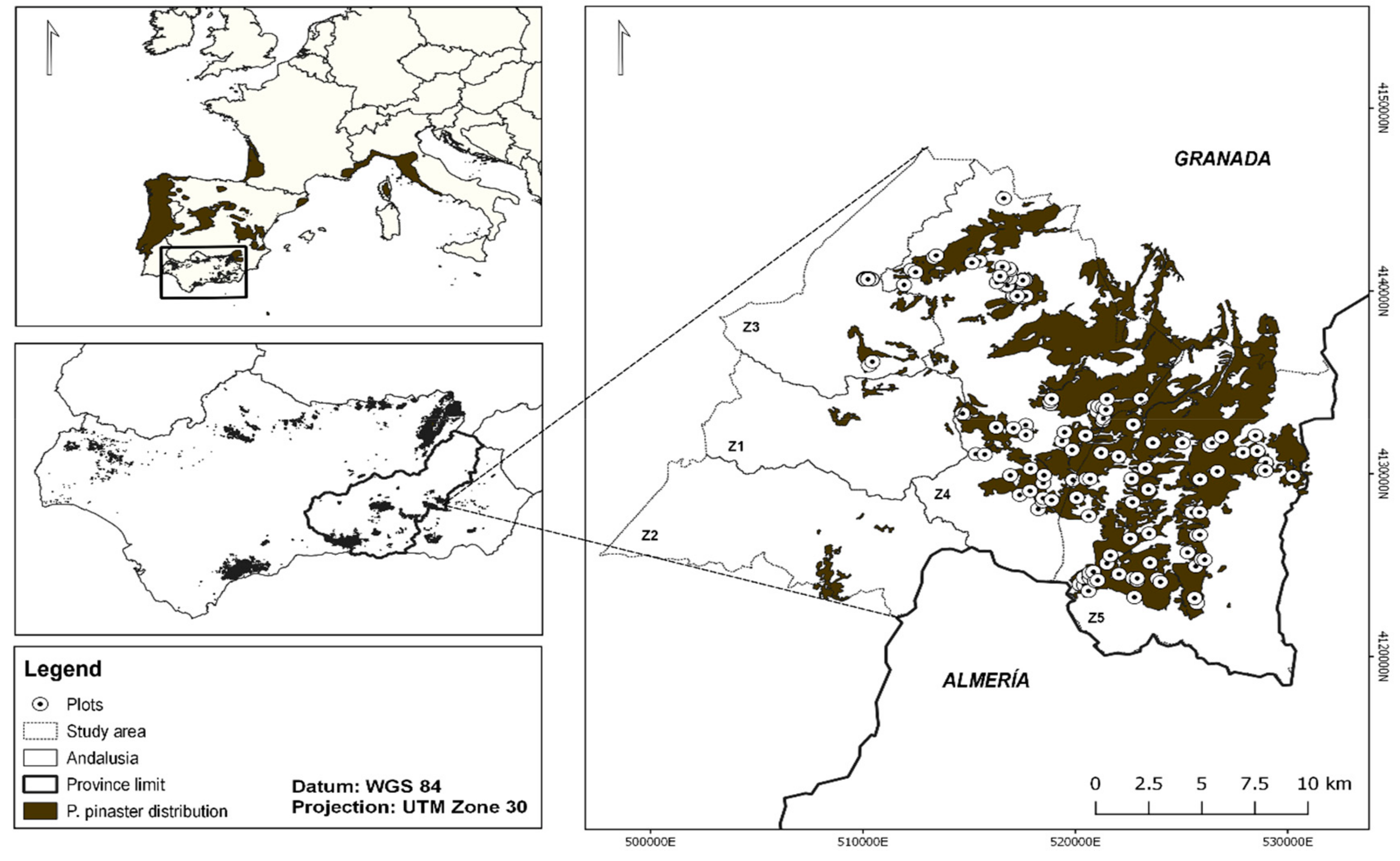
Figure 1. Location of Pinus pinaster forests in Sierra de Baza (37°13′N, 2°32′W) and sampled plots (N = 64; circles). A map showing the distribution of Maritime pine in the western Mediterranean Basin (upper inset left, brown area) with a square (black box) indicating the study area in SE Spain (Andalusia-Granada, lower inset left).
Remotesensing 11 02291 g001
Figure 2. Flowchart describing the methodological steps to integrate Landsat time-series of Normalized Burn Ratio (NBR) and hydrological modeling to assess the forest defoliation of Pinus pinaster Aiton., in south-eastern Spain.
Remotesensing 11 02291 g002
Figure 3. Global error and overall accuracy values of The Normalized Burn Ratio (NBR); Moisture Stress Index (MSI); Optimized Soil Adjusted Vegetation Index (OSAVI); Normalized Difference Vegetation Index (NDVI); and Enhanced Vegetation Index (EVI) for classification defoliation grades of Pinus pinaster forests obtained through hold-out cross-validation (NN: Neural Networks).
Remotesensing 11 02291 g003
Figure 4. Spearman´s correlation coefficients obtained by comparing defoliation (proxi NBR) and hydrological variables for Pinus pinaster forests affected by the defoliation process in Sierra de Baza (Andalusia-Granada). In (a), the variables were then computed for the hydrological year (01 October to September 30, inclusive), and (b) mean values were then computed at the seasonal scale. At the right of dashed line, hydrological variables related to the soil water content. Dotted lines are significant values (p < 0.05). See Table S1 for a list of the variables.
Remotesensing 11 02291 g004
Figure 5. Out-of-bag (OOB) error obtained in the prediction defoliation model of Maritime pine stands in a decline process in the variance, reached a local optimum, including the 80% of the data in the training set. Importance of environmental predictors in predicting the presence or absence of defoliation in southeastern Andalusia (Spain). Importance is measured by Random Forest (RF).
Remotesensing 11 02291 g005
Figure 6. Comparison of the predicted NBR and the real NBR of 255 tested points in the period 1996–2017. The solid line was the regressed line of the sample points with the least square regression method (see also Table S3 for the whole period 1984–2017).
Remotesensing 11 02291 g006
Table 1. Vegetation indices (VIs) considered in the study of Maritime pine stands in decline process in Sierra de Baza (Andalusia-Granada).
AcronymVegetation IndexEquationReferences
EVIEnhanced Vegetation Index 2.5 × NIR RED ( NIR + C 1 RED C 2 BLUE ) + L [47]
MSIMoisture Stress Index SWIR 1 NIR [48]
NBRNormalized Burn Ratio ( NIR SWIR 2 ) ( NIR + SWIR 2 ) [49]
NDVINormalized Difference Vegetation Index ( NIR RED ) ( NIR + RED ) [50]
OSAVIOptimized Soil Adjusted Vegetation Index ( 1 + L ) ( NIR RED ) ( NIR + RED + 0.16 ) [51]
Table 2. Summary of the statistical criteria computed for the evaluation of regression models used to study the defoliation of Pinus pinaster forests in Sierra de Baza (Southern Spain, Andalusia-Granada). Root Mean Squared Error (RMSE); average error (AVE), R-squared (R2), Spearman´s ρ (S) and root-mean-squared error of the cross-validation (RMSECV).
ModelRMSEAVER2SRMSECV
Random Forest0.06520.01120.79930.70300.0595
Support Vector Machines0.06420.00360.70460.58610.0731
Neural Network0.0737−0.00960.71110.50120.0714