Article

Toward Quantifying Oil Contamination in Vegetated Areas Using Very High Spatial and Spectral Resolution Imagery

1
Office National d’Études et de Recherches Aérospatiales (ONERA), 31055 Toulouse, France
2
TOTAL S.A., Pôle d’Études et de Recherches de Lacq, 64170 Lacq, France
3
EcoLab, Université de Toulouse, CNRS, INPT, UPS, 31062 Toulouse, France
4
DynaFor, Université de Toulouse, INRA, 31326 Castanet-Tolosan, France
5
TOTAL S.A., Centre Scientifique et Technique Jean-Féger, 64000 Pau, France
*
Author to whom correspondence should be addressed.
Remote Sens. 2019, 11(19), 2241; https://doi.org/10.3390/rs11192241
Submission received: 9 September 2019 / Revised: 24 September 2019 / Accepted: 25 September 2019 / Published: 26 September 2019
(This article belongs to the Special Issue Monitoring Soil Degradation by Remote Sensing)

Abstract

:
Recent remote sensing studies have suggested exploiting vegetation optical properties for assessing oil contamination, especially total petroleum hydrocarbons (TPH) in vegetated areas. Methods based on the tracking of alterations in leaf biochemistry have been proposed for detecting and quantifying TPH under controlled and field conditions. In this study, we expand their use to airborne imagery, in order to monitor oil contamination at a larger scale. Airborne hyperspectral images with very high spatial and spectral resolutions were acquired over an industrial site with oil-contamination (mud pits) and control sites both colonized by Rubus fruticosus L. The method of oil detection exploiting 14 vegetation indices succeeded in classifying the sites in the case of high TPH contamination (overall accuracy ≥ 91.8%). Two methods, based on either the PROSAIL (PROSPECT + SAIL) radiative transfer model or elastic net multiple regression, were also developed for quantifying TPH. Both methods were tested on reflectance measurements in the field, at leaf and canopy scales, and on the image, and achieved accurate predictions of TPH concentrations (RMSE ≤ 3.28 g/kg−1 and RPD ≥ 1.90). The methods were validated on additional sites and open up promising perspectives of operational application for oil and gas companies, with the emergence of new hyperspectral satellite sensors.

Graphical Abstract

1. Introduction

Since the beginning of the 20th century, oil and gas supply has constantly increased to satisfy a growing demand worldwide [1,2]. Along with the development of the oil industry, important efforts have been made to mitigate the associated environmental risks [3,4,5]. Oil spills and leakages are of major concern in the onshore domain. They are likely to occur at every step of the production process (i.e., oil extraction, refining, and transportation) contaminating the soil and groundwater and remaining as mud pits after their cessation [6,7,8]. The resulting soil contamination causes important ecological alterations (e.g., landscape fragmentation and habitat loss) [9,10,11,12]. To avoid such consequences, fast and accurate detection and quantification of oil contamination are, therefore, necessary.
Total petroleum hydrocarbons (TPH) are good indicators of oil contamination in soils [13,14]. They are the main constituent of oil and show high toxicity toward organisms. (In this study, the terms oil and TPH were used indifferently.) Among the methods proposed for detecting and quantifying TPH contamination, hyperspectral remote sensing has become a promising one [15,16]. Recent advances in this field allow monitoring industrial facilities (e.g., pipelines and storage tanks) at a large scale using airborne or satellite imagery [17,18], however, this approach is based on the detection of apparent oil at the surface, so its application in vegetated regions remains impossible. This causes a critical issue in regions with dense vegetation and intensive oil production activities. In this context, alternative approaches based on exploiting vegetation optical properties have emerged during the last decade [8,19,20,21,22].
TPH induce strong alterations in leaf anatomy and biochemistry related to their optical properties in the reflective domain (400–2500 nm) [23,24,25,26,27]. These alterations lead to modifications in the spectral signature of vegetation and suggest being able to detect oil in vegetated areas using optical remote sensing [28,29,30]. On the basis of this assumption, a few studies have attempted to map oil spills and leakages using multi- and hyperspectral airborne or satellite imagery with four to 30 m spatial resolution (mainly Landsat, Hyperion, and Hymap systems) [8,19,31,32]. Most of them have relied on comparisons of vegetation indices between healthy and contaminated sites, but only a few have proposed a method to detect oil contamination automatically, and even fewer have evaluated its performance. In addition, none of these studies attempted to quantify TPH. In most cases, the method of detection was applied to entire images [19,32]. This gave rise to the apparition of false alarms, caused by differences in species’ sensitivity to oil, bare soil-mixed vegetation pixels, and the presence of other vegetation stressors (e.g., water deficit). False alarms have been more pronounced using multispectral satellite imagery. Thus, several conclusions emerged from these studies. First, very high spatial (1–2 m) and spectral (<10 nm) resolutions are needed to achieve accurate detection of oil. Then, prior application to entire images, i.e., it is necessary to calibrate the methods over restricted areas with known species and contamination. Then, the methods should be validated on spatially independent sites with the same species and, as a last step, applied to entire images, provided that the target species’ location is known.
Species established around industrial oil facilities are naturally tolerant to soil contamination and difficult to distinguish from healthy vegetation [33,34]. It is, therefore, challenging to develop methods for detecting and quantifying TPH adapted to these species and intended to be applied to airborne and satellite hyperspectral images. Detecting and quantifying TPH is even more difficult in the presence of other environmental factors (e.g., water deficit). As suggested in previous work, this could be achieved by experiments carried out under controlled conditions [28,35]. Several studies have aimed to characterize the effects of oil on vegetation reflectance under controlled conditions [29,36,37,38]. Vegetation indices and spectrum transformations (first and second derivatives, continuum removal) have been frequently used for this purpose [20,30,38,39,40]. The wavelengths linked to pigment and water contents were particularly suitable for distinguishing healthy and oil-exposed vegetation with no or minor confusion [21,34]. More recently, Lassalle et al. [28] succeeded in discriminating among various types of oil contamination at leaf and canopy scales using vegetation indices. The same approach performed well for detecting mud pits contaminated by TPH in the field, by exploiting the reflectance of an oil-tolerant species (Rubus fruticosus L.). Radiative transfer models also sparked great interest for tracking alterations in leaf pigment contents caused by oil. For example, Arellano et al. [41] inverted the PROSPECT model [42] to detect changes in leaf chlorophyll content (LCC) resulting from an oil spill under tropical region. The same model was recently used for quantifying TPH in mud pit soils from leaf reflectance measurements performed in the field [43]. As suggested, its coupling with the SAIL canopy model [44] (forming the PROSAIL model [45]) might be of great interest for quantifying oil contamination in vegetated areas, from hyperspectral images. This challenge remains, however, very difficult, as it implies being able to track subtle changes in LCC from airborne or satellite sensors.
In the continuity of the abovementioned studies [28,43], this work aims to detect and quantify oil contamination (i.e., soil TPH content) in vegetated areas using airborne hyperspectral images with very high spatial and spectral resolutions. To achieve this, a method of detection previously developed under controlled conditions, hereafter summarized, was first applied to the images. Then, two approaches, either PROSAIL or multiple regression, are proposed to quantify TPH. Both were assessed in the field and on airborne hyperspectral images, on selected vegetation patches with known species.

2. Materials and Methods

2.1. Study Area and Soil Sampling

The study was carried out in a temperate region, on an industrial area subject to important oil and gas activities. During the past 50 years, oil production residues were accumulated in mud pits, which resulted in contamination of soil by TPH. Some of these mud pits remain and have been colonized by oil-tolerant vegetation, mainly Rubus fruticosus L. (bramble) (Figure 1c). The study focused on this species, as it is generally well-established in temperate industrial areas. Bramble served for developing the methods of oil detection and quantification under controlled and field conditions [28,34,43] and was suitable for application to hyperspectral imagery.
Five mud pits were identified for the study (Figure 1a), and the largest one (approximately 40 × 100 m, hereafter described as “brownfield”) was used for calibrating the methods. Within this site, 10 homogeneous and spatially correlated plots of 16 to 20 m2, mainly covered by R. fruticosus (>95%), were defined in the field (Figure 1b). Their geographical coordinates were acquired, and soil analyses were performed in two locations of each plot. Analyses revealed C10-C40 TPH concentrations ranging from 17 to 39 g/kg−1 on the site. The same sampling procedure was carried out on the four other mud pits, which were not spatially correlated with the brownfield. A single plot was defined on each of them, since they occupied a much smaller area. One of these mud pits exhibited comparable TPH concentrations (24 g/kg−1) (Table 1) and low concentrations were found in the other mud pits (≤3.15 g/kg−1). More information about the mud pits, including soil properties, can be found in our previous studies [28,34,43]. In addition, one large (~ 20 × 20 m) and five smaller control sites colonized by R. fruticosus were identified in the same region and used for the calibration and validation of the detection method, respectively, Figure 1d–f. No TPH were detected in soil analyses for any of the control sites. These sites, however, differed slightly in soil properties, especially in texture and the surrounding ecosystem (poplar plantation, grassland, and riparian forest). They were thus suitable for assessing the robustness of the method of detection.

2.2. Hyperspectral Data Acquisition and Preprocessing

2.2.1. Airborne Images

Hyperspectral images were acquired over the study area on July 5, 2017 at 1:15 p.m., at 2103 m above sea level in the absence of cloud, using airborne VNIR-1600 and SWIR-320m-e HySpex cameras (Norsk Elektro Optikk AS, Lørenskog, Norway) (Figure 1a,d). These images had a spatial resolution of 1 and 2.5 m and a spectral resolution of 5.2 and 7.8 nm in the visible-near infrared (VNIR, 400–1000 nm) and short-wave infrared (SWIR, 1000–2500 nm) domains, respectively. The SWIR image was resampled to 1 m spatial resolution using a nearest neighborhood filter, in order to preserve the spatial information, and registered according to the VNIR image using the Gefolki algorithm [46]. The resulting spectral radiance image was then converted to spectral reflectance using the empirical line method (ELM) [47,48], because of the lack of knowledge about the composition of the local industrial atmosphere. This provided a 1 m resampled reflectance image with 409 spectral bands covering the reflective domain (400–2500 nm). Because of the low signal-to-noise ratio (SNR), we did not conserve the bands with atmospheric transmission below 80%, as described in [49]. A Savitzky–Golay smoothing filter [50] was applied to improve the SNR at the remaining bands, and the final 1 m georeferenced reflectance image was used for calibrating and validating the methods of detection and quantification described hereafter.

2.2.2. Field Reflectance

On the day of image acquisitions, a field campaign was carried out on the 10 plots of the large mud pit (“brownfield”) (Figure 1b). On each plot, 18 and 9 spectral signatures of brambles were acquired at leaf and canopy scales, respectively, using an ASD FieldSpec 4 Hi-Res spectroradiometer (Malvern Panalytical, Malvern, UK). Data were acquired in radiance between 11:30 a.m. and 2:00 p.m. and converted to reflectance, as described in [28]. Leaf measurements were performed with a leaf clip. Canopy reflectance was acquired using a 25 mm wide fore optics placed 45 cm above the target at nadir, providing a 20 cm wide acquisition footprint. All spectral signatures were then resampled to the spectral resolution of the airborne image and the same band removal and smoothing procedures (atmospheric transmittance <80% and Savitzky–Golay smoothing filter) were applied. These data were used for calibrating the method of TPH quantification.

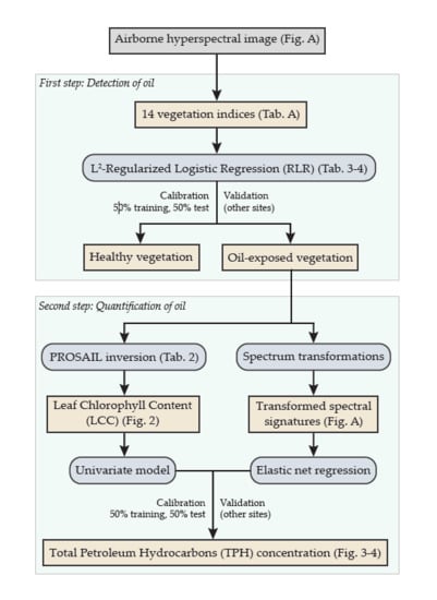
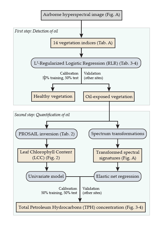
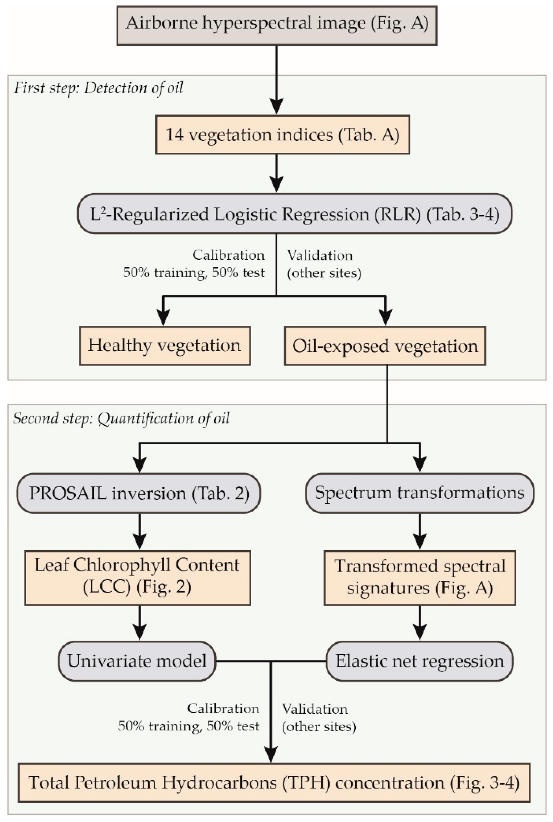
2.3. First Step of the Approach: Detection of Oil Contamination

A comprehensive flowchart of this study is presented in Figure A2 in the Appendix A. The approach proposed in this study is divided into the following two successive steps: (1) the detection of oil contamination and (2) the quantification of TPH. The first one relies on the application of a method previously developed in the same context of study, under controlled conditions. The method exploits 14 vegetation indices, computed from the spectral signatures, and the L2 regularized logistic regression (RLR) [51] classifier to determine whether vegetation is, or has been, exposed to oil (see [28] for a detailed description of the method). These indices have been linked to the effects specifically induced by oil on leaf pigment and water contents of bramble. They are listed in Table A1 in the Appendix A. The method succeeded in detecting oil contamination under controlled conditions, at leaf and canopy scales [28]. It has been validated under natural conditions on the brownfield, and therefore, in this study, we focused on its application to the airborne hyperspectral image.
The method was first tested on the 10 plots of the brownfield and on the large control site (Figure 1b,e). The corresponding spectral signatures were extracted from the image and the 14 vegetation indices were computed. Data were split into 50% training and 50% test sets using the Kennard–Stone algorithm [52], with an equal proportion of pixels from the brownfield and the control site in each. The RLR classifier was fitted on the training set and applied to the test set. Predictions made on the test set were evaluated using the overall accuracy (OA), Cohen’s kappa coefficient, and confusion matrices [49,53,54]. The method was then validated on the other contaminated and control sites (n = 4 and 5 sites, respectively, Table 1).

2.4. Second Step of the Approach: Quantification of Soil TPH Content

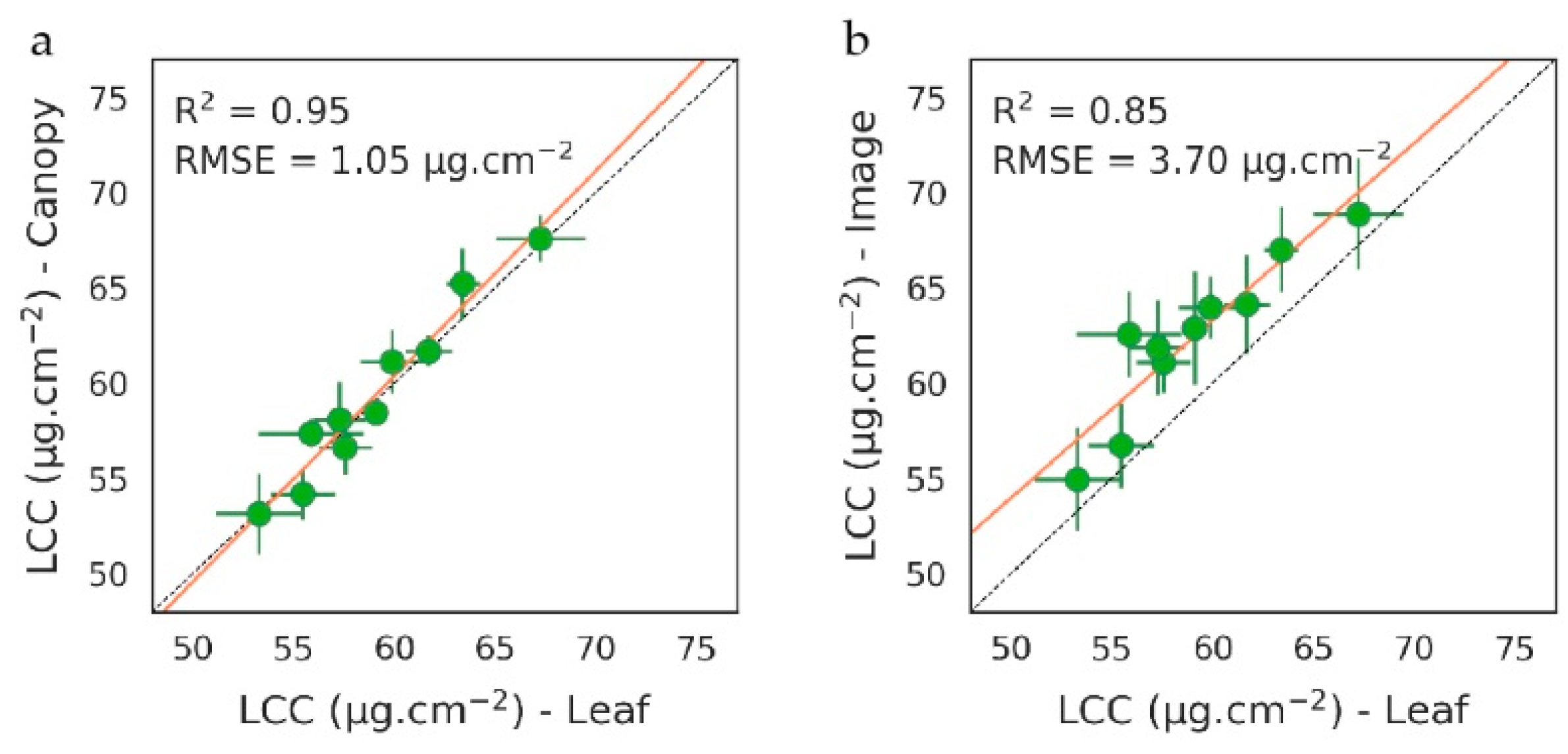
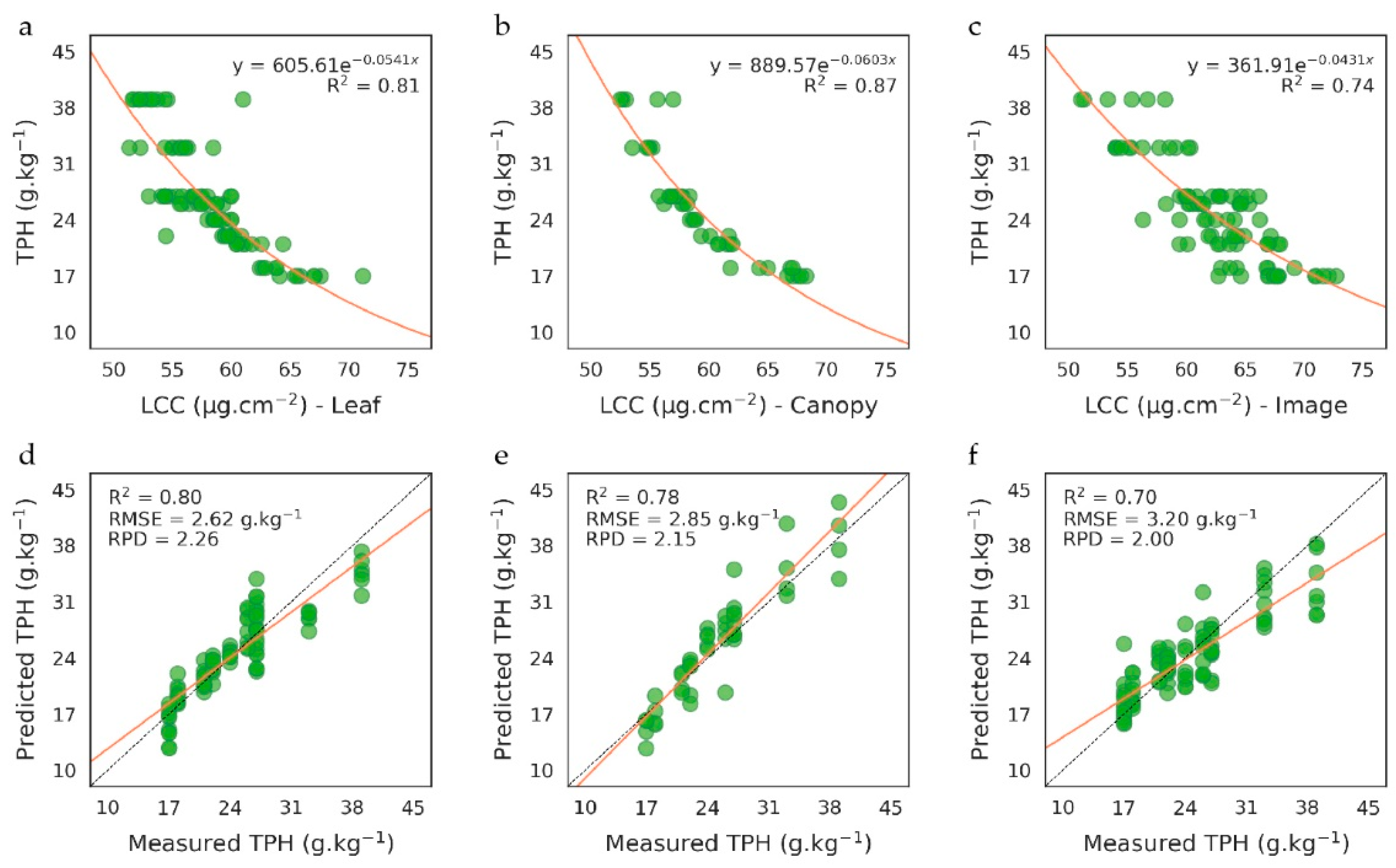
2.4.1. First Method Based on PROSPECT and PROSAIL

The first method proposed for quantifying soil TPH content relies on the retrieval of LCC by inverting the PROSPECT and PROSAIL radiative transfer models [42,44,45]. The PROSPECT model simulates the hemispherical reflectance and transmittance spectra of leaves in the reflective domain, knowing their biophysical and biochemical parameters (listed in Table 2). The model can be inverted to retrieve these parameters from reflectance measurements, using an iterative optimization approach [55,56]. The latter consists in successively testing different sets of parameters (denoted by the vector θ) and retaining the one that best simulates the measured spectral signature [57,58]. This is achieved by minimizing the cost function J, defined as:
J ( θ ) = λ min λ max ( R meas ( λ )     R sim ( λ ,   θ ) ) 2 ,
where Rsim and Rmeas denote the simulated and measured reflectance in the [λminmax] spectral range, respectively. In previous work, the LCC of R. fruticosus estimated using PROSPECT inversion was consistent with laboratory analyses and strongly linked to TPH concentrations [43]. This method was developed in the field and performed well for predicting the contamination level (i.e., TPH concentration) at leaf scale. In this study, we propose to assess its robustness on field measurements performed at canopy scale and on the airborne images, using the PROSAIL model. PROSAIL results from the coupling of PROSPECT and SAIL models [45]. It expands the scope of PROSPECT to dense canopy reflectance data by taking the influence of canopy architecture, leaf area index (LAI) and bare soil, and illumination and viewing geometry into account [59,60]. The inversion of the model follows the same procedure as that of PROSPECT. In this study, PROSAIL was used for retrieving LCC.
The principle of this method is to quantify TPH from LCC, so we applied it to the contaminated sites. PROSPECT was inverted on leaf reflectance measurements performed on the 10 plots of the brownfield (n = 180). On the same plots, PROSAIL was inverted on both field canopy measurements (n = 90) and on the pixels from the airborne image (n = 184). Inversions were computed using the differential evolution algorithm [43,61] and the model parameters listed in Table 2. The LCC values retrieved from canopy measurements and from the image were compared to those of leaves using the R2 and the root mean square error (RMSE) [43].
LCC was then used for quantifying TPH. Each data type (leaf, canopy, and image) was split into 50% training and 50% test sets. Negative exponential models were fitted between LCC and TPH concentrations on the training set and then applied to the test set [43]. TPH predictions were compared to the measured concentrations by computing the R2, the RMSE, and the residual predictive deviation (RPD) [66,67]. Since the method was calibrated for TPH concentrations ranging from 17 to 39 g/kg−1, it was validated on the mud pit with 24 g/kg−1 TPH only.

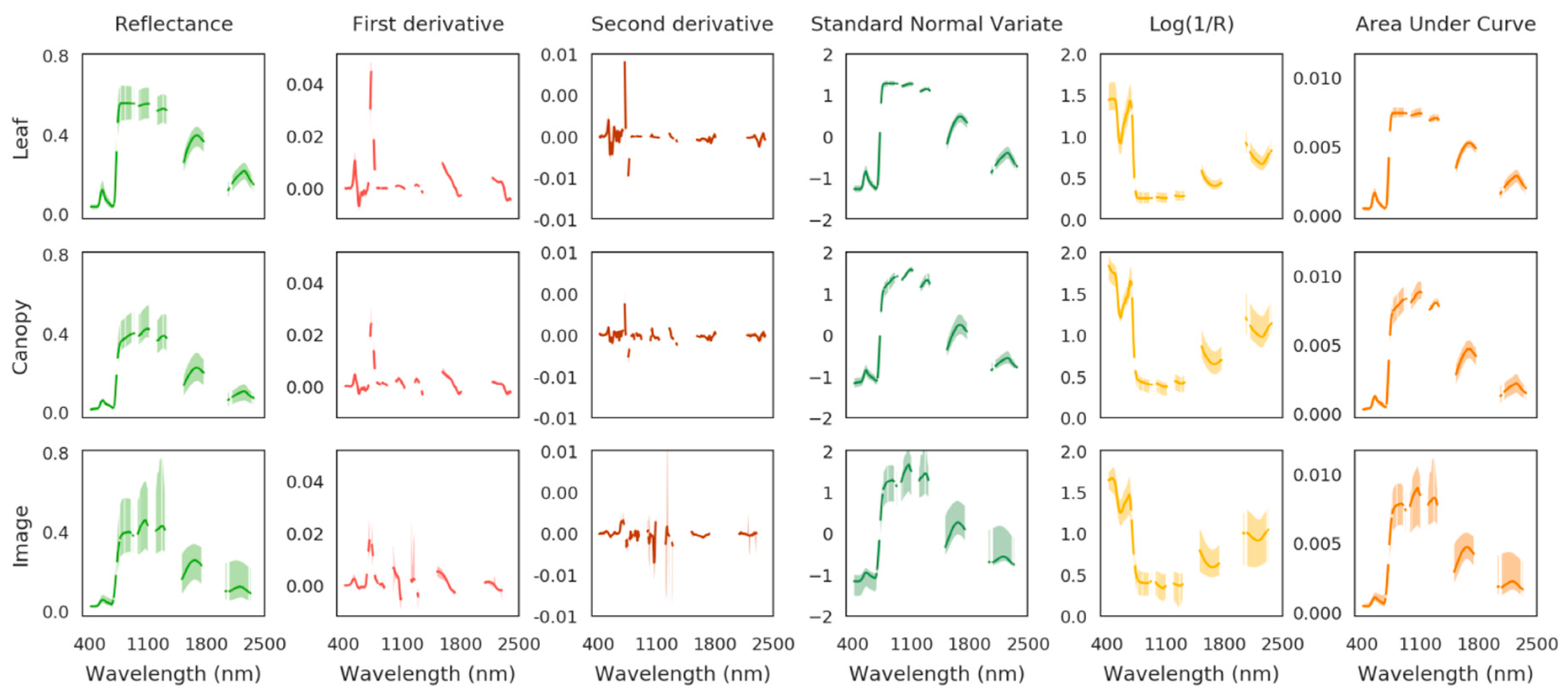
2.4.2. Second Method Based on Elastic Net Regression

The second method of quantification consists of linking the spectral signatures to TPH concentrations directly using multiple regression. Several approaches have been proposed in previous studies aiming to quantify heavy metals from vegetation reflectance in the field, especially partial least square regression (PLSR) [66,68]. PLSR is not suitable for TPH quantification [43], therefore, in this study, we proposed another regression approach, the elastic net (ENET [69]), which shows multiple advantages but remains underexploited in remote sensing of vegetation [70,71]. ENET is a penalized least squared approach that allows efficient variable selection under multicollinearity, which is a major limitation of other multiple regression approaches when dealing with hyperspectral data. Moreover, ENET performed well for tracking alterations in leaf biochemistry induced by oil in a previous study [28].
In the present study, ENET was used for predicting TPH concentration from the spectral signature of vegetation while selecting the most contributing spectral bands. For this purpose, several spectrum transformations were tested which included first and second derivatives, standard normal variate (SNV), Log(1/R), and area under curve normalization (AUCN) (see [34,66,72] for a detailed description of the transformations). All these transformations are likely to enhance the information contained in the spectral signature and to improve TPH predictions. They are illustrated in Figure A1 in the Appendix A. The method was applied to the spectral signatures acquired in the field (at leaf and canopy scales) and on the airborne image, following the same procedure as the PROSAIL method (i.e., training and test steps on the brownfield and validation on the other mud pits). The accuracy of TPH predictions were compared between the two methods, as well as their respective advantages.

3. Results

3.1. Calibration of the Methods

3.1.1. Detection of Oil Contamination

The RLR-based method exploiting vegetation indices performed well for discriminating between healthy and oil-exposed vegetation from the airborne image. The classification trained on the 10 zones of the brownfield and the large control site reached OA and Kappa of 98% and 0.95 on the test set, respectively. Only little confusions were made between healthy and oil-exposed vegetation (Table 3). Within the brownfield, the misclassified pixels came from the least contaminated plots (17–18 g/kg−1). Almost all pixels from the large control site were correctly classified. These results were consistent with those of previous studies carried out under controlled and field conditions on the same species, at leaf and canopy scales [28,34].
The robustness of the method to upscaling (i.e., at leaf and canopy scales and imagery) is due to the limited influence of plant architecture, bare soil, and illuminating and viewing geometry on the selected vegetation indices at high spatial resolution. These factors usually affect the ability of vegetation indices to detect changes in leaf biochemistry from canopy measurements or optical images [73,74,75]. This phenomenon was likely to induce confusion between healthy and oil-exposed vegetation, however, the 14 indices used in the method have been specifically selected for their robustness to upscaling and their link with oil-induced effects on leaf biochemistry [76,77,78]. These indices mainly depend on chlorophylls a and b, β-carotene, and lutein contents for bramble [28] (see Table A1 in the Appendix A). They are weakly affected by the abovementioned factors (especially bare soil). Therefore, they allow tracking alterations in leaf pigment contents specifically induced by oil with good accuracy, regardless of the acquisition scale [28].

3.1.2. Quantification of Soil TPH Content

PROSAIL-Based Method

LCC estimated from the inversions of PROSPECT and PROSAIL models on the 10 plots of the brownfield is presented in Figure 2. LCC estimations were strongly consistent among data types (i.e., leaf, canopy, and airborne image), especially in the field (R2 = 0.95 and RMSE = 1.05 µg/cm−2, Figure 2a) and ranged from 53 to 69 µg/cm−2, which is particularly high for vegetation exposed to contamination. This highlights the tolerance of bramble to oil exposure and explains its establishment on industrial sites under temperate regions [36,43,79,80]. PROSAIL is a one-layer model adapted to dense vegetation. Its application to the airborne image succeeded in retrieving LCC, thanks to very high spatial resolution. As expected, estimations were slightly less accurate and showed a higher variability within the plots than for field measurements (R2 = 0.85, RMSE = 3.70 µg/cm−2, Figure 2b).
LCC exhibited a close negative relationship with soil TPH content on the training set (0.74 < R2 < 0.87, Figure 3a–c). The more the soil was contaminated, the more LCC decreased. This relationship has been previously noticed under controlled conditions for oil-sensitive species and has been linked to the reduction of water and nutrient availability in soil and the alteration of root uptake capacities [23,81,82]. Similar observations have been made under natural conditions on bramble at leaf scale [43]. However, our method is the first to bring evidence of this relationship at leaf and canopy scales and on airborne images. Its application to the test set resulted in accurate predictions of TPH concentrations (Figure 3d–f). Results were very close at leaf and canopy scales (RMSE = 2.62 and 2.85 g/kg−1 and RPD = 2.26 and 2.15, respectively), thanks to consistent LCC described above (Figure 2a). A higher variability in LCC was observed on the image and led to a lower accuracy in TPH predictions (RMSE = 3.2 g/kg−1 and RPD = 2), in comparison to field measurements. The highest level of contamination (39 g/kg−1) was more difficult to predict and contributed considerably to inaccuracies. As previously observed at leaf scale, TPH are particularly difficult to quantify above a certain concentration [43], probably because variations in LCC become too subtle to be caught from imagery. In contrast, LCC rapidly shifts for moderate levels of contamination (20–30 g/kg−1) and makes predictions more accurate.

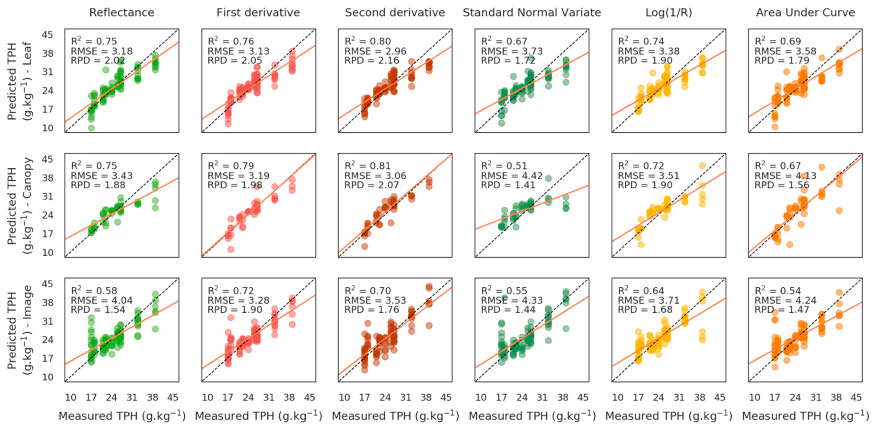
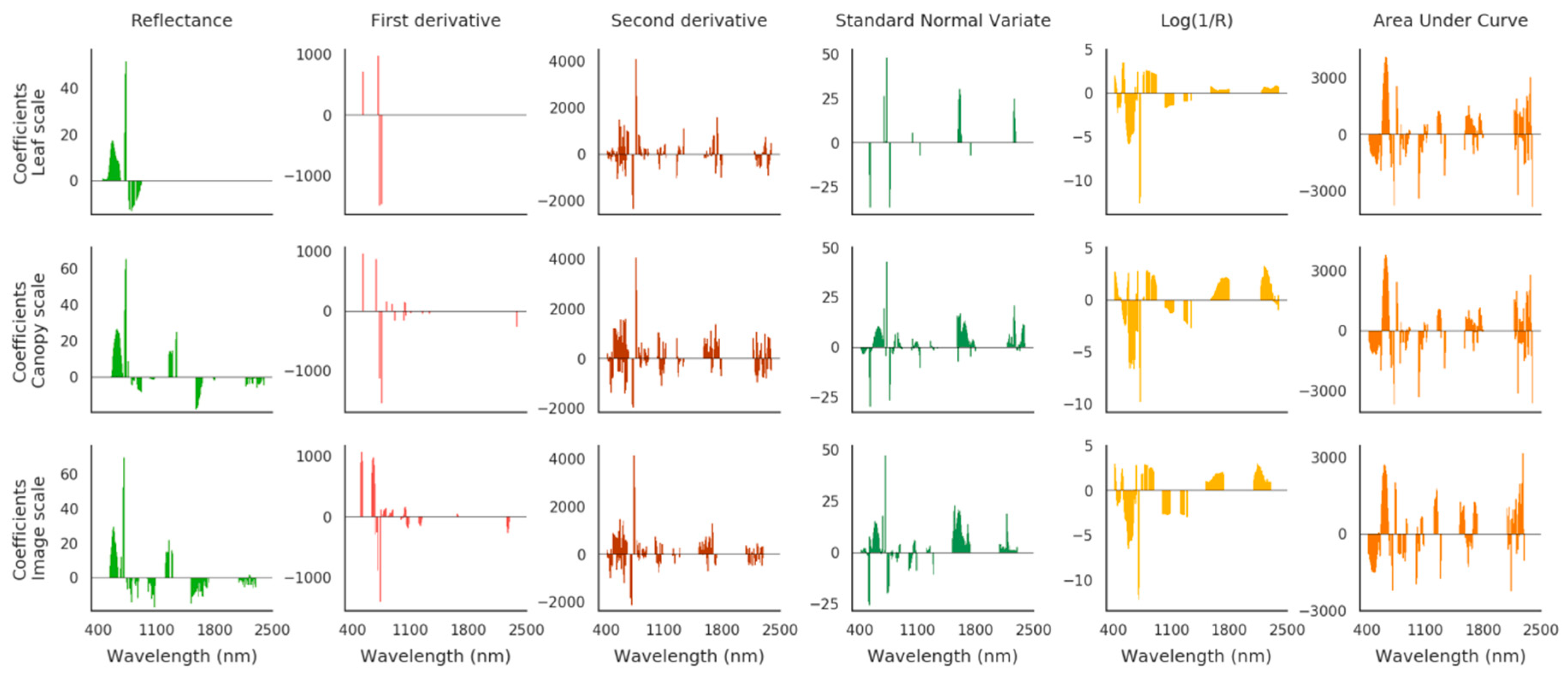
Elastic Net Based Method

The ENET regression based on the original and transformed spectral signatures also succeeded in predicting TPH concentrations on the brownfield (Figure 4). However, the overall performance of the method was lower than that based on PROSPECT and PROSAIL inversions, regardless of the transformation. Although TPH predictions were good for the original-reflectance-spectra for all scales (RMSE ≤ 4.04 g/kg−1), they were improved using first and second derivatives (RMSE ≤ 3.53 g/kg−1), mainly due to better quantification of the highest level of contamination (39 g/kg−1) at canopy scale and on the airborne image. Conversely, predictions were almost unchanged with the Log(1/R) transformation and less accurate using SNV and AUCN ones. As for the PROSPECT and PROSAIL based method, the accuracy of predictions was reduced while increasing acquisition scale (best RPD = 2.16, 2.07 and 1.9 at leaf and canopy scales and on the image, respectively, Figure 4).
Spectrum transformations have been extensively used for detecting vegetation stress in various contexts, including oil contamination [30,34,83,84]. The first derivative sparked particular interest, as it allows tracking shifts in the red edge position (REP) caused by chlorophyll alteration [20,29,85]. Therefore, the REP has been many times depicted as a reliable indicator of alterations in vegetation health following exposure to TPH [86], however, many other environmental stressors also affect the REP [22,83], which might lead to inaccuracies in TPH quantification. In our case, the ENET method highlighted the importance of the red edge, and to a greater extent the VIS region, for quantifying TPH, since most contributing bands were concentrated around 550 and 700 nm. This trend remained consistent among data types (leaf, canopy, and image) and between reflectance and derivative spectra (Figure 5), and therefore confirmed the involvement of chlorophylls in the response of vegetation to oil. The red edge was almost sufficient alone for predicting TPH using first derivative spectra, especially at leaf and canopy scales. Additional spectral bands from the SWIR region were often selected on the airborne image. These bands have been linked to leaf water, cellulose, and lignin contents in previous studies [87,88], but remained of less contribution to TPH predictions in our case. In contrast, SNV, Log(1/R), and AUCN transformation degraded TPH predictions, and did not provide a clear interpretation of the contributing spectral bands (Figure 5). These transformations are usually employed for reducing the high variability of spectral signatures while enhancing the information they contain [34,66]. In our case, reflectance varied little along the gradient of TPH (≤10% at 550 nm and in the red edge), because of the strong tolerance of bramble to oil exposure, in comparison to other species [20,30]. SNV, Log(1/R), and AUCN transformations were unable to conserve this information in the transformed spectra, which introduced inaccuracies in TPH predictions.

3.2. Validation of the Methods

3.2.1. Validation of Oil Detection

When applied to the validation sites, the method of oil detection based on the vegetation indices succeeded in detecting healthy vegetation. The ecological differences among the sites (soil properties and surrounding ecosystem) were challenging, because they could introduce variability in reflectance, and thus in index values, however, this had only a little influence on the performance of the method, since more than 91% of the pixels from the five control sites used for validation were correctly labelled (OA = 91.8%, Table 4). Conversely, the level of oil contamination was critical for the detection of mud pits. Accuracy averaged 50.5% on the four validation mud pits and resulted from strong differences among sites. As expected, the most contaminated one (24 g/kg−1) was well classified (95.5%), as it was in the range of the method calibration (17–39 g/kg−1). Conversely, accuracy rapidly fell for the other mud pits, where low TPH concentrations were observed. More precisely, the two least contaminated sites (0.25 and 0.38 g/kg−1 TPH) were poorly classified (accuracy of 6.1% and 15%, respectively, Table 4), because vegetation indices from these sites exhibited values similar to that of the control ones. These results emphasize the limits of the method. Below a certain concentration, oil no longer alters leaf pigment and water contents, so soil contamination becomes very difficult to detect using vegetation reflectance [21,28,30]. This detection limit strongly depends on the sensitivity of the species, and is higher for oil-tolerant species [20,33,38,89]. Thus, the closer the level of contamination to this limit, the less accurate the classification. In our case, this level was probably below the detection limit for bramble in the two least contaminated sites. Conversely, the method performed well for detecting the fourth validation mud pit contaminated by 3.15 g/kg−1 TPH. More than 85% of pixels from this site were correctly labelled, despite its contamination level being outside the calibration range. Hence, oil still induces important effects on leaf biochemistry of bramble at moderate contamination levels, which can be detected using the proposed method.

3.2.2. Validation of TPH Quantification

The two methods of quantification were applied to the mud pit contaminated by 24 g/kg−1 TPH and confirmed their potential for application to airborne hyperspectral images. The TPH concentrations were estimated to 23.69 (± 1.93) and 23.39 (± 2.41) g/kg−1 using PROSAIL inversions and ENET with first derivative spectra, respectively. Predictions were slightly less accurate using other spectrum transformations (SNV, Log(1/R), and AUCN), but remained very close to the measured level of contamination (data not shown). Both methods, thus, provide reliable quantification of TPH in the context of our study. It is, however, important to note that the concentration observed on this mud pit corresponded to that for which best predictions were obtained on the brownfield (Figure 3 and Figure 4). This explains the high accuracy of predictions observed here. Unfortunately, none of the four validation mud pits exhibited TPH concentrations above 35 g/kg−1 which was probably the most difficult to predict. It was thus not possible to validate the methods for such concentrations, but an underestimation would be probably observed, as on the brownfield. More generally, some inaccuracies in both methods of quantification might result from local variations in soil TPH content. These local variations introduce variability in bramble reflectance and might have affected TPH predictions, as suspected at leaf scale in previous study [43].

4. Discussion and Perspectives

To date, there was no remote sensing method for both detecting and quantifying oil contamination in vegetated areas based on hyperspectral imagery [19,31,32]. Our study is the first to achieve it using very high spatial resolution images acquired in a temperate region. This opens up encouraging perspectives for application of the methods over oil industrial facilities. In a perspective of operational use, it is essential that remote sensing provides reliable detection and quantification of oil over large vegetated areas. Until now, the proposed methods remained poorly effective outside the calibration site [19,32,90], making them unusable operationally. Conversely, those developed in this study were successfully validated, by detecting and quantifying oil on independent mud pits that did not serve for method calibration. Our methods were, however, applied under several assumptions. Since we focused on R. fruticosus in the temperate context, the methods were only adapted to this species. Thus, they could be applied for identifying new contaminated mud pits and for quantifying TPH, provided the sites are colonized by dense R. fruticosus covers with known location. This is of great interest for monitoring contamination, because this species is widespread on industrial sites under temperate regions [36,79,91]. In an operational perspective, the methods should be applicable at a large scale (i.e., to entire images) in a wide range of contexts (in terms of species, contamination type and level, and environmental conditions). No extensive computational time was noticed in this study, but this should be considered when applying our methods to entire images. Thanks to a good revisit time and large spatial coverage [22], satellite-embedded sensors show great interest for monitoring oil contamination continuously over industrial facilities, however, our methods were tested on a single date, so they should be first validated over a longer time scale [22,43]. In addition, to date, none of the operating and planned hyperspectral satellite-embedded sensors covering the reflective domain offer a spatial resolution higher than 8 m with more than 250 spectral bands. It is highly probable that, when applying our methods to satellite imagery, changes in spatial and spectral resolutions will affect their performance. Thus, in order to support oil exploration and contamination monitoring, the methods should improve in two ways. First, by extending their scope, and then, by adapting them to satellite imagery. These two perspectives are discussed jointly in this section.
At this stage, the need to know the location of R. fruticosus is one of the most important limits to the application of the methods at a large scale. The mapping of R. fruticosus could be achieved quite easily for homogenous and dense covers, such as those studied here. Conversely, R. fruticosus is more likely to be mixed with other species and bare soil in pixels using satellite imagery, affecting the values of the 14 VI used in the detection method and consequently reducing its accuracy. Likewise, PROSAIL inversions might experience difficulties in retrieving LCC accurately for sparse of plurispecific vegetation, because of the influence of bare soil and differences in optical properties, leaf orientation, and sensitivity to oil among species [45,62]. In response to this limit, spectral unmixing [92,93,94,95] seems a promising solution. It could be used for mapping R. fruticosus, even mixed with bare soil or other species, before applying our methods of oil detection and quantification. A successful mapping of R. fruticosus has been achieved using unmixing methods on HyMap images (spatial resolution < 10 m) in a previous study [95]. Future studies should focus on assessing unmixing methods on known sites with this species, for example by degrading 1 m spatial resolution airborne images to 8 m and 30 m resolution. In that sense, it might be interesting not to limit to a single species in our case. This would be spatially too restrictive from an operational point of view, so an important effort remains to adapt our methods to other species. Other temperate species might serve for detecting and quantifying oil,- such as Q. pubescens and P. canadensis, as highlighted in our previous study [43]. Thus, they could be used along with R. fruticosus for assessing mud pit contamination at a large scale, after being identified by spectral unmixing.
Even if the methods can be applied to entire images, provided that the target species have been identified, it is important to note that their performance depends on the level of contamination. With respect to R. fruticosus, the method of detection was initially adapted to a high TPH concentration (≥17 g/kg−1). Satisfying accuracy was obtained for low-contaminated mud pit (3.15 g/kg−1 TPH), but accuracy fell below 1 g/kg−1 TPH. This helped determining a lower detection limit. Conversely, the method of quantification based on LCC retrieval was accurate within the range of TPH studied. Its exact range of effectiveness remains, however, unknown. Thus, further research should focus on determining the exact limits of detection and quantification of the methods. These limits may vary among species, depending on their sensitivity. All of them do not allow detecting and quantifying mud pit contamination in the same range. Species with different sensitivities could be complementary for quantifying TPH over a wide range of concentrations. Spatial resolution might be also crucial, especially if TPH concentrations vary locally. In the case of 8 m or 30 m satellite imagery, pixels may include vegetation exposed to varying levels of contamination, making it difficult to quantify accurately. An important effort still remains to determine which species are suitable for applying the methods and their respective range of effectiveness at different spatial resolutions.
Although the scope of the methods is restricted to assessing mud pit contamination (i.e., production residues and oil sludge) at this stage, it should extend to other scenarios. Crude oil or petroleum product leaks deriving from pipeline or storage tank failures are a priority. Along with wastewater, they represent the main sources of contaminant release from oil industry [6,96]. Moreover, the detection of crude oil is of great interest in microseepage prospecting. This represents a major way of improvements toward operational applications. From the perspective of operational application, one possible limit to applying our methods may arise at the spatial resolution of satellite images for punctual oil patches. Microseepage and mud pits generally occupy large areas (>30 m), but pipeline and storage tank leaks can occur on a few square meters [17,97]. Their detection might be very difficult without very high spatial resolution, because pixels will rarely include only oil-exposed vegetation. Thus, it is important to keep in mind that the needed spatial resolution also depends on the purpose of the detection and quantification of oil.

5. Conclusions

This study aimed to detect and quantify oil contamination (i.e., TPH) in soils in temperate vegetated areas using airborne imagery with very high spatial and spectral resolutions. A two-step approach was proposed. As a first step, a method of detection exploiting 14 vegetation indices performed well for discriminating between healthy and oil-exposed bramble plants (OA = 98% and kappa = 0.95). This method was tested on additional sites and succeeded in detecting oil contamination levels similar to those of the calibration site (17–39 g/kg−1). Then, the performance of the method decreased for lower levels of contaminations, especially below 1 g/kg−1. As a second step, two methods of TPH quantification were proposed and assessed on the same contaminated sites. The first one, which relied on LCC retrieval using PROSPECT and PROSAIL models, achieved accurate predictions of TPH concentrations both in the field, at leaf and canopy scales, and on the airborne image (RMSE ≤ 3.20 g/kg−1 and RPD ≥ 2), thanks to consistent LCC estimations. The second method combined spectrum transformations with ENET regression. This method provided slightly less accurate quantification of TPH (best RMSE ≤ 3.28 g/kg−1 and RPD ≥ 1.9) and required only few spectral bands in the VIS and the red edge regions. Both methods were validated on another contaminated site and their performances were compared.
In the continuity of previous work, this multiscale study highlighted the importance of controlled and field conditions for developing reliable methods that can be applied to hyperspectral imagery. Our methods focused on tracking oil-induced alterations in leaf biochemistry while preventing from undesired effects (plant architecture, bare soil, and illuminating and viewing geometry), which made them accurate regardless of the acquisition scale. High spatial resolution helped achieving this. As discussed above, further studies are needed to adapt our methods to various ecological contexts subject to oil contamination. In addition, promising perspectives of operational use will arise in the future with the emergence of new hyperspectral satellite sensors.

Author Contributions

Conceptualization, G.L., A.E., A.C., D.D. and S.F.; methodology, software, and validation, G.L.; formal analysis, G.L.; investigation, G.L., A.E., A.C., R.H., G.B., D.D. and S.F.; resources, S.F., A.C. and R.H.; data curation, G.L.; writing—original draft preparation, G.L.; writing—review and editing, G.L., A.E., A.C., G.B., D.D. and S.F.; visualization, G.L.; supervision, S.F., A.E. and D.D.; project administration, G.L., A.E., A.C., D.D. and S.F.; funding acquisition, A.C. and D.D.

Funding

This research was funded by TOTAL.

Acknowledgments

This work was performed in the frame of the NAOMI project between TOTAL and the ONERA, with the support of the EcoLab and the DynaFor research units of Toulouse. The authors gratefully acknowledge V. Tardivat for the field access authorizations; V. Achard, K. Adeline, and P. Borderies for their assistance in field sampling; and P. Déliot and L. Poutier for their implication in image acquisitions and atmospheric correction.

Conflicts of Interest

The authors declare no conflict of interest.

Appendix A

Table A1. Vegetation indices used in the method of detection. For each index, the related biochemical parameters are specified. These parameters have been identified in a previous study carried out on R. fruticosus, under controlled conditions [28]. (Chl, total chlorophylls; Lut, lutein; B-car, β-carotene; Ant, antheraxanthin; Zea, zeaxanthin; Vio, violaxanthin; and LWC, leaf water content).
IndexFormulaReferenceRelated Farameter
Chlorophyll/Carotenoids Index CCI = D 720 / D 700 [98]Chl, B-car
Carter Index 2 CTR 2 = R 695 / R 760 [99]Chl, Lut
Gitelson & Merzlyak Index 1 GM 1 = R 750 / R 550 [77]Chl, B-car
Gitelson & Merzlyak Index 2 GM 2 = R 750 / R 700 [77]Chl, B-car
modified Simple Ratio 705 nm mSR 705 = ( R 750 R 445 ) / ( R 750 + R 445 ) [26]Chl, B-car
MERIS Terrestrial Chlorophyll Index MTCI = ( R 754 R 709 ) / ( R 709 + R 681 ) [76]Chl, B-car
Normalized Difference 705 nm ND 705   or   NDVI 705   = ( R 750 R 705 ) / ( R 750 + R 705 ) [26]Chl, B-car
Photochemical Reflectance Index 2 PRI 2 = ( R 531 R 570 ) / ( R 531 + R 570 ) [100]Chl, B-car
Photochemical Reflectance Index 3 PRI 3 = ( R 570 R 539 ) / ( R 570 + R 539 ) [100]Lut, B-car
Structure Intensive Pigment Index 2 SIPI 2 = ( R 800 R 505 ) / ( R 800 + R 690 ) [73]Lut, Ant
Simple Ratio 705 nm SR 705 = R 750 / R 705 [26]Chl, B-car
Vogelmann Index 2 VOG 2 = ( R 734 R 747 ) / ( R 715 + R 726 ) [78]Lut
Vogelmann Index 3 VOG 3 = ( R 734 R 747 ) / ( R 715 + R 720 ) [78]Lut
Disease Water Stress Index DWSI = ( R 800 R 550 ) / ( R 1660 + R 680 ) [101]LWC
Figure A1. Original and transformed spectral signatures acquired in the brownfield at leaf and canopy scales and from the airborne image. The bold curve represents the median spectral signature and the colored area represents the (min:max) interval.
Remotesensing 11 02241 g0a1
Figure A2. Flowchart of the approach proposed in this study. The method of oil detection was developed and tested at leaf and canopy scales in [28], so it was only evaluated on the airborne image in this study. The two methods of total petroleum hydrocarbons (TPH) quantification were tested in the field at leaf and canopy scales and on the airborne image. All the methods were first calibrated on study sites and validated on additional sites (see Table 1 for details about the sites).
Remotesensing 11 02241 g0a2

References

  1. Miller, R.G.; Sorrell, S.R.; Lane, H.; Kt, S. The future of oil supply. Philos. Trans. R. Soc. A 2014, 372, 20130179. [Google Scholar] [CrossRef] [PubMed] [Green Version]
  2. Sorrell, S.; Miller, R.; Bentley, R.; Speirs, J. Oil futures: A comparison of global supply forecasts. Energy Policy 2010, 38, 4990–5003. [Google Scholar] [CrossRef]
  3. Barraza, F.; Maurice, L.; Uzu, G.; Becerra, S.; López, F.; Ochoa-Herrera, V.; Ruales, J.; Schreck, E. Distribution, contents and health risk assessment of metal(loid)s in small-scale farms in the Ecuadorian Amazon: An insight into impacts of oil activities. Sci. Total Environ. 2018, 622–623, 106–120. [Google Scholar] [CrossRef] [PubMed]
  4. Shukla, A.; Karki, H. Application of robotics in onshore oil and gas industry—A review Part I. Rob. Auton. Syst. 2016, 75, 490–507. [Google Scholar] [CrossRef]
  5. Slonecker, T.; Fisher, G.B.; Aiello, D.P.; Haack, B. Visible and infrared remote imaging of hazardous waste: A review. Remote Sens. 2010, 2, 2474–2508. [Google Scholar] [CrossRef]
  6. Chang, J.I.; Lin, C.C. A study of storage tank accidents. J. Loss Prev. Process Ind. 2006, 19, 51–59. [Google Scholar] [CrossRef]
  7. Shadizadeh, S.R.; Zoveidavianpoor, M. A drilling reserve mud pit assessment in Iran: Environmental impacts and awareness. Pet. Sci. Technol. 2010, 28, 1513–1526. [Google Scholar] [CrossRef]
  8. Van der Werff, H.; van der Meijde, M.; Jansma, F.; van der Meer, F.; Groothuis, G.J. A Spatial-Spectral Approach for Visualization of Vegetation Stress Resulting from Pipeline Leakage. Sensors 2008, 8, 3733–3743. [Google Scholar] [CrossRef] [PubMed] [Green Version]
  9. Bi, X.; Wang, B.; Lu, Q. Fragmentation effects of oil wells and roads on the Yellow River Delta, North China. Ocean Coast. Manag. 2011, 54, 256–264. [Google Scholar] [CrossRef]
  10. Finer, M.; Jenkins, C.N.; Pimm, S.L.; Keane, B.; Ross, C. Oil and gas projects in the Western Amazon: Threats to wilderness, biodiversity, and indigenous peoples. PLoS ONE 2008, 3, e2932. [Google Scholar] [CrossRef]
  11. Jones, N.F.; Pejchar, L.; Kiesecker, J.M. The energy footprint: How oil, natural gas, and wind energy affect land for biodiversity and the flow of ecosystem services. Bioscience 2015, 65, 290–301. [Google Scholar] [CrossRef]
  12. Onyia, N.; Balzter, H.; Berrio, J.-C. Normalized Difference Vegetation Vigour Index: A New Remote Sensing Approach to Biodiversity Monitoring in Oil Polluted Regions. Remote Sens. 2018, 10, 897. [Google Scholar] [CrossRef]
  13. Kisic, I.; Mesic, S.; Basic, F.; Brkic, V.; Mesic, M.; Durn, G.; Zgorelec, Z.; Bertovic, L. The effect of drilling fluids and crude oil on some chemical characteristics of soil and crops. Geoderma 2009, 149, 209–216. [Google Scholar] [CrossRef]
  14. Wang, Z.; Fingas, M.; Page, D.S. Oil Spill Identification. J. Chromatogr. A 1999, 843, 369–411. [Google Scholar] [CrossRef]
  15. Correa Pabón, R.E.; de Souza Filho, C.R. Spectroscopic characterization of red latosols contaminated by petroleum-hydrocarbon and empirical model to estimate pollutant content and type. Remote Sens. Environ. 2016, 175, 323–336. [Google Scholar] [CrossRef]
  16. Scafutto, R.D.P.M.; de Souza Filho, C.R.; de Oliveira, W.J. Hyperspectral remote sensing detection of petroleum hydrocarbons in mixtures with mineral substrates: Implications for onshore exploration and monitoring. ISPRS J. Photogramm. Remote Sens. 2017, 128, 146–157. [Google Scholar] [CrossRef]
  17. Correa Pabón, R.E.; de Souza Filho, C.R.; Oliveira, W.J. de Reflectance and imaging spectroscopy applied to detection of petroleum hydrocarbon pollution in bare soils. Sci. Total Environ. 2019, 649, 1224–1236. [Google Scholar] [CrossRef] [PubMed]
  18. Hese, S.; Schmullius, C. High spatial resolution image object classification for terrestrial oil spill contamination mapping in West Siberia. Int. J. Appl. Earth Obs. Geoinf. 2009, 11, 130–141. [Google Scholar] [CrossRef]
  19. Arellano, P.; Tansey, K.; Balzter, H.; Boyd, D.S. Detecting the effects of hydrocarbon pollution in the Amazon forest using hyperspectral satellite images. Environ. Pollut. 2015, 205, 225–239. [Google Scholar] [CrossRef]
  20. Emengini, E.J.; Blackburn, G.A.; Theobald, J.C. Early detection of oil-induced stress in crops using spectral and thermal responses. J. Appl. Remote Sens. 2013, 7, 73596. [Google Scholar] [CrossRef]
  21. Gürtler, S.; de Souza Filho, C.R.; Sanches, I.D.; Alves, M.N.; Oliveira, W.J. Determination of changes in leaf and canopy spectra of plants grown in soils contaminated with petroleum hydrocarbons. ISPRS J. Photogramm. Remote Sens. 2018, 146, 272–288. [Google Scholar] [CrossRef]
  22. Gholizadeh, A.; Kopačková, V. Detecting vegetation stress as a soil contamination proxy: A review of optical proximal and remote sensing techniques. Int. J. Environ. Sci. Technol. 2019, 16, 2511–2524. [Google Scholar] [CrossRef]
  23. Baruah, P.; Saikia, R.R.; Baruah, P.P.; Deka, S. Effect of crude oil contamination on the chlorophyll content and morpho-anatomy of Cyperus brevifolius (Rottb.) Hassk. Environ. Sci. Pollut. Res. 2014, 21, 12530–12538. [Google Scholar] [CrossRef]
  24. Balliana, A.G.; Moura, B.B.; Inckot, R.C.; Bona, C. Development of Canavalia ensiformis in soil contaminated with diesel oil. Environ. Sci. Pollut. Res. 2017, 24, 979–986. [Google Scholar] [CrossRef] [PubMed]
  25. Nakata, C.; Qualizza, C.; MacKinnon, M.; Renault, S. Growth and physiological responses of Triticum aestivum and Deschampsia caespitosa exposed to petroleum coke. Water. Air. Soil Pollut. 2011, 216, 59–72. [Google Scholar] [CrossRef]
  26. Sims, D.A.; Gamon, J.A. Relationships between leaf pigment content and spectral reflectance across a wide range of species, leaf structures and developmental stages. Remote Sens. Environ. 2002, 81, 337–354. [Google Scholar] [CrossRef]
  27. Ustin, S.L.; Schaepman, M.E.; Gitelson, A.A.; Jacquemoud, S.; Schaepman, M.; Asner, G.P.; Gamon, J.A.; Zarco-Tejada, P. Retrieval of foliar information about plant pigment systems from high resolution spectroscopy. Remote Sens. Environ. 2009, 113, S67–S77. [Google Scholar] [CrossRef] [Green Version]
  28. Lassalle, G.; Fabre, S.; Credoz, A.; Hédacq, R.; Borderies, P.; Bertoni, G.; Erudel, T.; Buffan-Dubau, E.; Dubucq, D.; Elger, A. Detection and discrimination of various oil-contaminated soils using vegetation reflectance. Sci. Total Environ. 2019, 655, 1113–1124. [Google Scholar] [CrossRef] [PubMed]
  29. Rosso, P.H.; Pushnik, J.C.; Lay, M.; Ustin, S.L. Reflectance properties and physiological responses of Salicornia virginica to heavy metal and petroleum contamination. Environ. Pollut. 2005, 137, 241–252. [Google Scholar] [CrossRef]
  30. Sanches, I.D.; de Souza Filho, C.R.; Magalhães, L.A.; Quitério, G.C.M.; Alves, M.N.; Oliveira, W.J. Assessing the impact of hydrocarbon leakages on vegetation using reflectance spectroscopy. ISPRS J. Photogramm. Remote Sens. 2013, 78, 85–101. [Google Scholar] [CrossRef]
  31. Adamu, B.; Tansey, K.; Ogutu, B. Remote sensing for detection and monitoring of vegetation affected by oil spills. Int. J. Remote Sens. 2018, 39, 3628–3645. [Google Scholar] [CrossRef] [Green Version]
  32. Ozigis, M.S.; Kaduk, J.D.; Jarvis, C.H. Mapping terrestrial oil spill impact using machine learning random forest and Landsat 8 OLI imagery: A case site within the Niger Delta region of Nigeria. Environ. Sci. Pollut. Res. 2019, 26, 3621–3635. [Google Scholar] [CrossRef] [PubMed]
  33. Arellano, P.; Tansey, K.; Balzter, H.; Tellkamp, M. Plant family-specific impacts of petroleum pollution on biodiversity and leaf chlorophyll content in the Amazon rainforest of Ecuador. PLoS ONE 2017, 12, e0169867. [Google Scholar] [CrossRef] [PubMed]
  34. Lassalle, G.; Credoz, A.; Hédacq, R.; Fabre, S.; Dubucq, D.; Elger, A. Assessing Soil Contamination Due to Oil and Gas Production Using Vegetation Hyperspectral Reflectance. Environ. Sci. Technol. 2018, 52, 1756–1764. [Google Scholar] [CrossRef] [PubMed]
  35. Huang, S.; Chen, S.; Wang, D.; Zhou, C.; van der Meer, F.; Zhang, Y. Hydrocarbon micro-seepage detection from airborne hyper-spectral images by plant stress spectra based on the PROSPECT model. Int. J. Appl. Earth Obs. Geoinf. 2019, 74, 180–190. [Google Scholar] [CrossRef]
  36. Credoz, A.; Hédacq, R.; Barreau, C.; Dubucq, D. Experimental study of hyperspectral responses of plants grown on mud pit soil. In Proceedings of the Earth Resources and Environmental Remote Sensing/GIS Applications VII, Edinburgh, UK, 27–29 September 2016; Volume 10005, p. 100051E. [Google Scholar]
  37. Emengini, E.J.; Blackburn, G.A.; Theobald, J.C. Discrimination of plant stress caused by oil pollution and waterlogging using hyperspectral and thermal remote sensing. J. Appl. Remote Sens. 2013, 7, 73476. [Google Scholar] [CrossRef]
  38. Lassalle, G.; Credoz, A.; Fabre, S.; Elger, A.; Hédacq, R.; Dubucq, D. Hyperspectral signature analysis of three plant species to long-term hydrocarbon and heavy metal exposure. In Proceedings of the Earth Resources and Environmental Remote Sensing/GIS Applications VIII, Warsaw, Poland, 11–14 September 2017; Michel, U., Schulz, K., Eds.; SPIE: Bellingham, WA, USA, 2017; Volume 10428, p. 33. [Google Scholar]
  39. Noomen, M.F.; Skidmore, A.K.; van der Meer, F.D.; Prins, H.H.T. Continuum removed band depth analysis for detecting the effects of natural gas, methane and ethane on maize reflectance. Remote Sens. Environ. 2006, 105, 262–270. [Google Scholar] [CrossRef]
  40. Sanches, I.D.; Souza Filho, C.R.; Magalhães, L.A.; Quitério, G.C.M.; Alves, M.N.; Oliveira, W.J. Unravelling remote sensing signatures of plants contaminated with gasoline and diesel: An approach using the red edge spectral feature. Environ. Pollut. 2013, 174, 16–27. [Google Scholar] [CrossRef]
  41. Arellano, P.; Tansey, K.; Balzter, H.; Boyd, D.S. Field spectroscopy and radiative transfer modelling to assess impacts of petroleum pollution on biophysical and biochemical parameters of the Amazon rainforest. Environ. Earth Sci. 2017, 76, 1–14. [Google Scholar] [CrossRef]
  42. Jacquemoud, S.; Baret, F. PROSPECT: A model of leaf optical properties spectra. Remote Sens. Environ. 1990, 34, 75–91. [Google Scholar] [CrossRef]
  43. Lassalle, G.; Fabre, S.; Credoz, A.; Hédacq, R.; Bertoni, G.; Dubucq, D.; Elger, A. Application of PROSPECT for estimating total petroleum hydrocarbons in contaminated soils from leaf optical properties. J. Hazard. Mater. 2019, 377, 409–417. [Google Scholar] [CrossRef] [Green Version]
  44. Verhoef, W. Light scattering by leaf layers with application to canopy reflectance modeling: The SAIL model. Remote Sens. Environ. 1984, 16, 125–141. [Google Scholar] [CrossRef] [Green Version]
  45. Jacquemoud, S.; Verhoef, W.; Baret, F.; Bacour, C.; Zarco-Tejada, P.J.; Asner, G.P.; François, C.; Ustin, S.L. PROSPECT+SAIL models: A review of use for vegetation characterization. Remote Sens. Environ. 2009, 113, S56–S66. [Google Scholar] [CrossRef]
  46. Brigot, G.; Colin-Koeniguer, E.; Plyer, A.; Janez, F. Adaptation and Evaluation of an Optical Flow Method Applied to Coregistration of Forest Remote Sensing Images. IEEE J. Sel. Top. Appl. Earth Obs. Remote Sens. 2016, 9, 2923–2939. [Google Scholar] [CrossRef] [Green Version]
  47. Smith, G.M.; Milton, E.J. The use of the empirical line method to calibrate remotely sensed data to reflectance. Int. J. Remote Sens. 1999, 20, 2653–2662. [Google Scholar] [CrossRef]
  48. Roberts, D.A.; Smith, M.O.; Adams, J.B. Green vegetation, nonphotosynthetic vegetation, and soils in AVIRIS data. Remote Sens. Environ. 1993, 44, 255–269. [Google Scholar] [CrossRef]
  49. Erudel, T.; Fabre, S.; Houet, T.; Mazier, F.; Briottet, X. Criteria Comparison for Classifying Peatland Vegetation Types Using In Situ Hyperspectral Measurements. Remote Sens. 2017, 9, 748. [Google Scholar] [CrossRef]
  50. Savitzky, A.; Golay, M.J.E. Smoothing and Differentiation of Data by Simplified Least Squares Procedures. Anal. Chem. 1964, 36, 1627–1639. [Google Scholar] [CrossRef]
  51. Hoerl, A.E.; Kennard, R.W. Ridge regression: Biased estimation for nonorthogonal problems. Technometrics 1970, 12, 55–67. [Google Scholar] [CrossRef]
  52. Kennard, R.W.; Stone, L.A. Computer Aided Design of Experiments. In Technometrics; Palgrave Macmillan: London, UK, 1969; Volume 11, pp. 137–148. [Google Scholar]
  53. Story, M.; Congalton, R.G. Remote Sensing Brief Accuracy Assessment: A User’s Perspective. Photogramm. Eng. Remote Sens. 1986, 52, 397–399. [Google Scholar]
  54. Wei, C.; Huang, J.; Wang, X.; Blackburn, G.A.; Zhang, Y.; Wang, S.; Mansaray, L.R. Hyperspectral characterization of freezing injury and its biochemical impacts in oilseed rape leaves. Remote Sens. Environ. 2017, 195, 56–66. [Google Scholar] [CrossRef] [Green Version]
  55. Feret, J.B.; François, C.; Asner, G.P.; Gitelson, A.A.; Martin, R.E.; Bidel, L.P.R.; Ustin, S.L.; le Maire, G.; Jacquemoud, S. PROSPECT-4 and 5: Advances in the leaf optical properties model separating photosynthetic pigments. Remote Sens. Environ. 2008, 112, 3030–3043. [Google Scholar] [CrossRef]
  56. Féret, J.B.; Gitelson, A.A.; Noble, S.D.; Jacquemoud, S. PROSPECT-D: Towards modeling leaf optical properties through a complete lifecycle. Remote Sens. Environ. 2017, 193, 204–215. [Google Scholar] [CrossRef] [Green Version]
  57. Jacquemoud, S.; Baret, F.; Andrieu, B.; Danson, F.M.; Jaggard, K. Extraction of Vegetation Biophysical Parameters by Inversion of the PROSPECT + SAIL Models on Sugar Beet Canopy Reflectance Data. Application to TM and AVIRIS Sensors. Remote Sens. Environ. 1995, 52, 163–172. [Google Scholar] [CrossRef]
  58. Sun, J.; Shi, S.; Yang, J.; Du, L.; Gong, W.; Chen, B.; Song, S. Analyzing the performance of PROSPECT model inversion based on different spectral information for leaf biochemical properties retrieval. ISPRS J. Photogramm. Remote Sens. 2018, 135, 74–83. [Google Scholar] [CrossRef]
  59. Darvishzadeh, R.; Skidmore, A.; Schlerf, M.; Atzberger, C. Inversion of a radiative transfer model for estimating vegetation LAI and chlorophyll in a heterogeneous grassland. Remote Sens. Environ. 2008, 112, 2592–2604. [Google Scholar] [CrossRef]
  60. Zarco-Tejada, P.J.; Camino, C.; Beck, P.S.A.; Calderon, R.; Hornero, A.; Hernández-Clemente, R.; Kattenborn, T.; Montes-Borrego, M.; Susca, L.; Morelli, M.; et al. Previsual symptoms of Xylella fastidiosa infection revealed in spectral plant-trait alterations. Nat. Plants 2018, 4, 432–439. [Google Scholar] [CrossRef]
  61. Storn, R.; Price, K. Differential Evolution—A Simple and Efficient Heuristic for Global Optimization over Continuous Spaces. J. Glob. Optim. 1997, 11, 341–359. [Google Scholar] [CrossRef]
  62. Berger, K.; Atzberger, C.; Danner, M.; D’Urso, G.; Mauser, W.; Vuolo, F.; Hank, T. Evaluation of the PROSAIL model capabilities for future hyperspectral model environments: A review study. Remote Sens. 2018, 10, 85. [Google Scholar] [CrossRef]
  63. Botha, E.J.; Leblon, B.; Zebarth, B.; Watmough, J. Non-destructive estimation of potato leaf chlorophyll from canopy hyperspectral reflectance using the inverted PROSAIL model. Int. J. Appl. Earth Obs. Geoinf. 2007, 9, 360–374. [Google Scholar] [CrossRef]
  64. Si, Y.; Schlerf, M.; Zurita-Milla, R.; Skidmore, A.; Wang, T. Mapping spatio-temporal variation of grassland quantity and quality using MERIS data and the PROSAIL model. Remote Sens. Environ. 2012, 121, 415–425. [Google Scholar] [CrossRef]
  65. Balandier, P.; Marquier, A.; Casella, E.; Kiewitt, A.; Coll, L.; Wehrlen, L.; Harmer, R. Architecture, cover and light interception by bramble (Rubus fruticosus): A common understorey weed in temperate forests. Forestry 2013, 86, 39–46. [Google Scholar] [CrossRef]
  66. Shi, T.; Liu, H.; Wang, J.; Chen, Y.; Fei, T.; Wu, G. Monitoring arsenic contamination in agricultural soils with reflectance spectroscopy of rice plants. Environ. Sci. Technol. 2014, 48, 6264–6272. [Google Scholar] [CrossRef] [PubMed]
  67. Wang, J.; Wang, T.; Skidmore, A.K.; Shi, T.; Wu, G. Evaluating different methods for grass nutrient estimation from canopy hyperspectral reflectance. Remote Sens. 2015, 7, 5901–5917. [Google Scholar] [CrossRef]
  68. Zhou, C.; Chen, S.; Zhang, Y.; Zhao, J.; Song, D.; Liu, D. Evaluating Metal Effects on the Reflectance Spectra of Plant Leaves during Different Seasons in Post-Mining Areas, China. Remote Sens. 2018, 10, 1211. [Google Scholar] [CrossRef]
  69. Zou, H.; Hastie, T. Regression and variable selection via the elastic net. J. R. Stat. Soc. Ser. B (Stat. Methodol.) 2005, 67, 301–320. [Google Scholar] [CrossRef]
  70. Hong, Y.; Chen, Y.; Yu, L.; Liu, Y.; Liu, Y.; Zhang, Y.; Liu, Y.; Cheng, H. Combining fractional order derivative and spectral variable selection for organic matter estimation of homogeneous soil samples by VIS-NIR spectroscopy. Remote Sens. 2018, 10, 479. [Google Scholar] [CrossRef]
  71. Prospere, K.; McLaren, K.; Wilson, B. Plant species discrimination in a tropical wetland using in situ hyperspectral data. Remote Sens. 2014, 6, 8494–8523. [Google Scholar] [CrossRef]
  72. Peng, X.; Shi, T.; Song, A.; Chen, Y.; Gao, W. Estimating soil organic carbon using VIS/NIR spectroscopy with SVMR and SPA methods. Remote Sens. 2014, 6, 2699–2717. [Google Scholar] [CrossRef]
  73. Blackburn, G.A. Quantifying chlorophylls and carotenoids at leaf and canopy scales: An evaluation of some hyperspectral approaches. Remote Sens. Environ. 1998, 66, 273–285. [Google Scholar] [CrossRef]
  74. Broge, N.H.; Leblanc, E. Comparing prediction power and stability of broadband and hyperspectral vegetation indices for estimation of green leaf area index and canopy chlorophyll density. Remote Sens. Environ. 2000, 76, 156–172. [Google Scholar] [CrossRef]
  75. Verrelst, J.; Schaepman, M.E.; Koetz, B.; Kneubühler, M. Angular sensitivity analysis of vegetation indices derived from CHRIS/PROBA data. Remote Sens. Environ. 2008, 112, 2341–2353. [Google Scholar] [CrossRef]
  76. Dash, J.; Curran, P.J. Evaluation of the MERIS terrestrial chlorophyll index (MTCI). Adv. Space Res. 2007, 39, 100–104. [Google Scholar] [CrossRef]
  77. Gitelson, A.A.; Merzlyak, M.N. Remote estimation of chlorophyll content in higher plant leaves. Int. J. Remote Sens. 1997, 18, 2691–2697. [Google Scholar] [CrossRef]
  78. Zarco-Tejada, P.J.; Miller, J.R.; Noland, T.L.; Mohammed, G.H.; Sampson, P.H. Scaling-up and model inversion methods with narrowband optical indices for chlorophyll content estimation in closed forest canopies with hyperspectral data. IEEE Trans. Geosci. Remote Sens. 2001, 39, 1491–1507. [Google Scholar] [CrossRef] [Green Version]
  79. Nujkić, M.M.; Dimitrijević, M.M.; Alagić, S.Č.; Tošić, S.B.; Petrović, J.V. Impact of metallurgical activities on the content of trace elements in the spatial soil and plant parts of Rubus fruticosus L. Environ. Sci. Process. Impacts 2016, 18, 350–360. [Google Scholar] [CrossRef] [PubMed] [Green Version]
  80. Yoon, J.; Cao, X.; Zhou, Q.; Ma, L.Q. Accumulation of Pb, Cu, and Zn in native plants growing on a contaminated Florida site. Sci. Total Environ. 2006, 368, 456–464. [Google Scholar] [CrossRef]
  81. Athar, H.R.; Ambreen, S.; Javed, M.; Hina, M.; Rasul, S.; Zafar, Z.U.; Manzoor, H.; Ogbaga, C.C.; Afzal, M.; Al-Qurainy, F.; et al. Influence of sub-lethal crude oil concentration on growth, water relations and photosynthetic capacity of maize (Zea mays L.) plants. Environ. Sci. Pollut. Res. 2016, 23, 18320–18331. [Google Scholar] [CrossRef]
  82. Han, G.; Cui, B.X.; Zhang, X.X.; Li, K.R. The effects of petroleum-contaminated soil on photosynthesis of Amorpha fruticosa seedlings. Int. J. Environ. Sci. Technol. 2016, 13, 2383–2392. [Google Scholar] [CrossRef] [Green Version]
  83. Smith, K.L.L.; Steven, M.D.D.; Colls, J.J.J. Use of hyperspectral derivative ratios in the red-edge region to identify plant stress responses to gas leaks. Remote Sens. Environ. 2004, 92, 207–217. [Google Scholar] [CrossRef]
  84. Zarco-Tejada, P.J.; Pushnik, J.C.; Dobrowski, S.; Ustin, S.L. Steady-state chlorophyll a fluorescence detection from canopy derivative reflectance and double-peak red-edge effects. Remote Sens. Environ. 2003, 84, 283–294. [Google Scholar] [CrossRef]
  85. Zhu, L.; Chen, Z.; Wang, J.; Ding, J.; Yu, Y.; Li, J.; Xiao, N.; Jiang, L.; Zheng, Y.; Rimmington, G.M. Monitoring plant response to phenanthrene using the red edge of canopy hyperspectral reflectance. Mar. Pollut. Bull. 2014, 86, 332–341. [Google Scholar] [CrossRef] [PubMed]
  86. van der Meer, F.; van Dijk, P.; van der Werff, H.; Yang, H. Remote sensing and petroleum seepage: A review and case study. Terra Nov. 2002, 14, 1–17. [Google Scholar] [CrossRef]
  87. Sims, D.A.; Gamon, J.A. Estimation of vegetation water content and photosynthetic tissue area from spectral reflectance: A comparison of indices based on liquid water and chlorophyll absorption features. Remote Sens. Environ. 2003, 84, 526–537. [Google Scholar] [CrossRef]
  88. Wang, Z.; Skidmore, A.K.; Wang, T.; Darvishzadeh, R.; Hearne, J. Applicability of the PROSPECT model for estimating protein and cellulose+lignin in fresh leaves. Remote Sens. Environ. 2015, 168, 205–218. [Google Scholar] [CrossRef]
  89. Emengini, E.J.; Ezeh, F.C.; Chigbu, N. Comparative Analysis of Spectral Responses of Varied Plant Species to Oil Stress. Int. J. Sci. Eng. Res. 2013, 4, 1421–1427. [Google Scholar]
  90. Noomen, M.F.; van der Werff, H.M.A.; van der Meer, F.D. Spectral and spatial indicators of botanical changes caused by long-term hydrocarbon seepage. Ecol. Inform. 2012, 8, 55–64. [Google Scholar] [CrossRef]
  91. Dorrington, V.H.; Pyatt, F.B. Some aspects of tissue accumulation and tolerance to available heavy metal ions by Rubus Fruticosus L., A Colonizer of spoil tips in S.W. England. Int. J. Environ. Stud. 1983, 20, 229–237. [Google Scholar] [CrossRef]
  92. Bioucas-Dias, J.M.; Plaza, A.; Dobigeon, N.; Parente, M.; Du, Q.; Gader, P.; Chanussot, J. Hyperspectral unmixing overview: Geometrical, statistical, and sparse regression-based approaches. IEEE J. Sel. Top. Appl. Earth Obs. Remote Sens. 2012, 5, 354–379. [Google Scholar] [CrossRef]
  93. Zhong, Y.; Zhao, L.; Zhang, L. An adaptive differential evolution endmember extraction algorithm for hyperspectral remote sensing imagery. IEEE Geosci. Remote Sens. Lett. 2014, 11, 1061–1065. [Google Scholar] [CrossRef]
  94. Stagakis, S.; Vanikiotis, T.; Sykioti, O. Estimating forest species abundance through linear unmixing of CHRIS/PROBA imagery. ISPRS J. Photogramm. Remote Sens. 2016, 119, 79–89. [Google Scholar] [CrossRef]
  95. Dehaan, R.; Louis, J.; Wilson, A.; Hall, A.; Rumbachs, R. Discrimination of blackberry (Rubus fruticosus sp. agg.) using hyperspectral imagery in Kosciuszko National Park, NSW, Australia. ISPRS J. Photogramm. Remote Sens. 2007, 62, 13–24. [Google Scholar] [CrossRef]
  96. Cunha, S.B. da A review of quantitative risk assessment of onshore pipelines. J. Loss Prev. Process Ind. 2016, 44, 282–298. [Google Scholar] [CrossRef]
  97. Asadzadeh, S.; de Souza Filho, C.R. Spectral remote sensing for onshore seepage characterization: A critical overview. Earth-Science Rev. 2017, 168, 48–72. [Google Scholar] [CrossRef] [Green Version]
  98. Sims, D.A.; Luo, H.; Hastings, S.; Oechel, W.C.; Rahman, A.F.; Gamon, J.A. Parallel adjustments in vegetation greenness and ecosystem CO2 exchange in response to drought in a Southern California chaparral ecosystem. Remote Sens. Environ. 2006, 103, 289–303. [Google Scholar] [CrossRef]
  99. Carter, G.A. Ratios of leaf reflectances in narrow wavebands as indicators of plant stress. Int. J. Remote Sens. 1994, 15, 517–520. [Google Scholar] [CrossRef]
  100. Gamon, J.A.J.A.; Peñuelas, J.; Field, C.B.B.; Penuelas, J.; Field, C.B.B. a Narrow-Waveband Spectral Index That Tracks Diurnal Changes in Photosynthetic Efficiency. Remote Sens. Environ. 1992, 41, 35–44. [Google Scholar] [CrossRef]
  101. Apan, A.; Held, A.; Phinn, S.; Markley, J. Detecting sugarcane ‘orange rust’ disease using EO-1 Hyperion hyperspectral imagery. Int. J. Remote Sens. 2004, 25, 489–498. [Google Scholar] [CrossRef]
Figure 1. (a,d) Subsets of the airborne hyperspectral image acquired over (a) the contaminated and (d) the control sites. The calibration sites are illustrated by polygons. Circles correspond to the validation sites (red: contaminated, white: control). (b,e) Zoom on (b) the brownfield (10 plots) and (e) the control sites used for calibrating the methods, respectively. (c,f) R. fruticosus on (c) the brownfield and (f) on the control site in March.
Remotesensing 11 02241 g001
Figure 2. (ab) Leaf chlorophyll content (LCC) (mean ± SD) retrieved from PROSPECT and PROSAIL model inversions on the 10 plots of the brownfield. (a) Comparison between leaf and canopy measurements from the field and (b) between leaf measurements and the airborne image.
Remotesensing 11 02241 g002
Figure 3. (ac) Relationship between LCC and soil total petroleum hydrocarbons (TPH) content observed on the training set on the 10 plots of the brownfield, at (a) leaf and (b) canopy scales and (c) on the airborne image. (df) Comparison between measured and predicted TPH concentrations on the test set, at (d) leaf and (e) canopy scales and (f) on the airborne image.
Remotesensing 11 02241 g003
Figure 4. Comparison between measured and predicted TPH concentrations on the test set on the 10 plots of the brownfield using the elastic net regression on the original and transformed spectral signatures (in columns). First, second, and third rows show the results obtained at leaf and canopy scales and on the airborne image, respectively.
Remotesensing 11 02241 g004
Figure 5. Coefficients obtained by the elastic net (ENET) method on the 10 plots of the brownfield using the original and transformed spectral signatures (in columns). First, second, and third rows show the results obtained at leaf and canopy scales and on the airborne image, respectively. The spectral bands contributing to TPH predictions are denoted by nonzero coefficients.
Remotesensing 11 02241 g005
Table 1. Description of the sites used for testing and validating the methods. (<DL, below detection limit).
StepZone TypeNumber of Zones (n)Total Pixel CountC10-C40 TPH (g/kg−1)
training + testcontrol1388<DL
training + testmud pit (“brownfield”)1018417–39
validationcontrol5211<DL
validationmud pit4330.25
200.38
483.15
2224
Table 2. Parameter bounds used to compute PROSPECT and PROSAIL (PROSPECT + SAIL) inversions.
ParameterUnitRangeReference
PROSPECT:
Leaf structure (N) 1–5[43]
Chlorophyll a + b (Cab)µg/cm−21–100
Carotenoids (Ccx)µg/cm−21–50
Brown pigments (Cbp)µg/cm−20.01–1
Water (Cw)g/cm−20.001–0.1
Dry matter (Cm)g/cm−20.001–0.1
SAIL:
Leaf Area Index (LAI)m2/m−20.1–5[59,60,62,63,64]
Hotspot (hot)m/m−10.01–0.1
Leaf Inclination Distribution Function (LIDF) Planophile 1
Soil brightness 2 (bright) 0.5–1.5
Solar zenith angle (θs)deg.Fixed (30°)
Viewing zenith angle (θv)deg.Fixed (0°)
Relative azimuth angle (φsv)deg.Fixed (0°)
1 As specified for Rubus fruticosus L. in [65]. 2 The recent version of PROSAIL includes a simple lambertian soil reflectance model. A brightness parameter (bright) was added to account for soil moisture and roughness [59,64].
Table 3. Confusion matrix obtained from the regularized logistic regression (RLR) classification on the test set using the 14 vegetation indices. The brownfield class denotes the pixels from the 10 zones of the brownfield, and the control denotes those from the large control site.
BrownfieldControlUser’s Accuracy (%)
Brownfield88495,7
Control219299.0
Producer’s accuracy (%)97.898.0
Table 4. Confusion matrix obtained from the RLR classification on the validation sites using the 14 vegetation indices.
C10-C40 TPH (g/kg−1)Mud PitControlUser’s Accuracy (%)
Control 1<DL1314691.8
Mud pit0.252316.1
0.3831715
3.1541785.4
2421195.5
1 The five control sites were grouped for more concision.

