Airborne Hyperspectral Imaging for Submerged Archaeological Mapping in Shallow Water Environments

Abstract

Nearshore areas around the world contain a wide variety of archeological structures, including prehistoric remains submerged by sea level rise during the Holocene glacial retreat. While natural processes, such as erosion, rising sea level, and exceptional climatic events have always threatened the integrity of this submerged cultural heritage, the importance of protecting them is becoming increasingly critical with the expanding effects of global climate change and human activities. Aerial archaeology, as a non-invasive technique, contributes greatly to documentation of archaeological remains. In an underwater context, the difficulty of crossing the water column to reach the bottom and its potential archaeological information usually requires active remote-sensing technologies such as airborne LiDAR bathymetry or ship-borne acoustic soundings. More recently, airborne hyperspectral passive sensors have shown potential for accessing water-bottom information in shallow water environments. While hyperspectral imagery has been assessed in terrestrial continental archaeological contexts, this study brings new perspectives for documenting submerged archaeological structures using airborne hyperspectral remote sensing. Airborne hyperspectral data were recorded in the Visible Near Infra-Red (VNIR) spectral range (400–1000 nm) over the submerged megalithic site of Er Lannic (Morbihan, France). The method used to process these data included (i) visualization of submerged anomalous features using a minimum noise fraction transform, (ii) automatic detection of these features using Isolation Forest and the Reed–Xiaoli detector and (iii) morphological and spectral analysis of archaeological structures from water-depth and water-bottom reflectance derived from the inversion of a radiative transfer model of the water column. The results, compared to archaeological reference data collected from in-situ archaeological surveys, showed for the first time the potential of airborne hyperspectral imagery for archaeological mapping in complex shallow water environments.

1. Introduction

Whether of natural (e.g., erosion, rising sea level and exceptional climatic events) or human (e.g., urbanization, agriculture, and pollution) origin, threats to archaeological heritage are increasingly significant [1,2]. Documenting and monitoring archaeological sites is consequently increasingly becoming a crucial aspect of conserving cultural heritage. In an underwater context, documenting archaeological remains requires mapping seabed details to interpret various forms of past human traces [3,4,5]. While much underwater archaeological research has been oriented to shipwrecks [5,6,7], nearshore areas contain a wide variety of ancient structures, including prehistoric remains submerged by the sea rise initiated 15,000 years ago by the Holocene glacial retreat. On a global scale, the now-submerged landscapes that were once attractive terrestrial habitats for prehistoric human occupation are estimated to cover ca. 20 million km² [8].

In the last few decades, active remote-sensing methods have successfully detected and recorded submerged archaeological sites in deep and shallow water. From the water surface, multibeam echo sounders (MBES) installed on hydrographic vessels or USV (unmanned surface vehicles) are used for archaeological applications. Despite high costs of operation and relatively low spatial coverage per time unit, MBES remain the preferred solution for seabed prospection, especially in deep water [9]. In coastal shallow waters, however, rock outcrops and rough sea conditions can reduce the potential area of operation due to safety issues, and multipath acoustic propagation interference also decreases the quality of acoustic measurements [10]. More recently, underwater hyperspectral imagers have also shown considerable potential for underwater archaeological surveys [11]; however, their use is limited to in-situ observations and low spatial coverage. Airborne LiDAR bathymetry (ALB) has gained great interest for underwater archaeological mapping [12,13,14]. When operated in topo-bathy mode, it can cover the intertidal zone and provide seamless representation of terrestrial and submerged topography. ALB has drawbacks, however, including relatively high deployment costs and difficulty in retrieving reliable depth measurements in very shallow water [15,16].

In comparison, passive remote-sensing data, such as multispectral or hyperspectral airborne and spatial imagery, have so far focused almost exclusively on terrestrial archaeological contexts. Airborne hyperspectral instruments measure, for a large number of pixels (millions) and wavelengths (tens to hundreds), the radiation (spectral radiance) received at the sensor. The data they collect are generally presented in the form of a data cube (2 spatial dimensions × 1 spectral dimension). Depending on sensor characteristics, the spectral dimension covers specific wavelength ranges, such as the Visible Near Infra-Red (VNIR) range, corresponding to wavelengths of 400–1000 nm. Due to its ability to acquire highly detailed spectral information, airborne hyperspectral imagery (AHI) has been used for various types of earth observation: land-cover/land-use mapping [17,18], target detection [19], geology [20] and coastal mapping [21]. For archaeological applications, airborne hyperspectral data have been greatly valuable for terrestrial mapping [22,23,24,25,26,27,28,29,30,31], but to our knowledge, no studies have yet assessed AHI in a submerged context. Using it for underwater mapping requires addressing challenges related to the complexity of (i) the data (including high dimensionality and signal-to-noise ratio), (ii) the object of study (degraded and partially documented structures) and (iii) the environment, especially the complex light-matter interactions in water, affected by multiple environmental factors such as water constituents, surface conditions and benthic composition.

Thus, the aim of this study was to evaluate the potential of AHI for detecting and documenting submerged sites in coastal archeology. The questions addressed are (a) can submerged archaeological structures be visible using AHI? (b) Can they be detected automatically? (c) Can they be characterized spatially and spectrally?

2. Materials and Methods

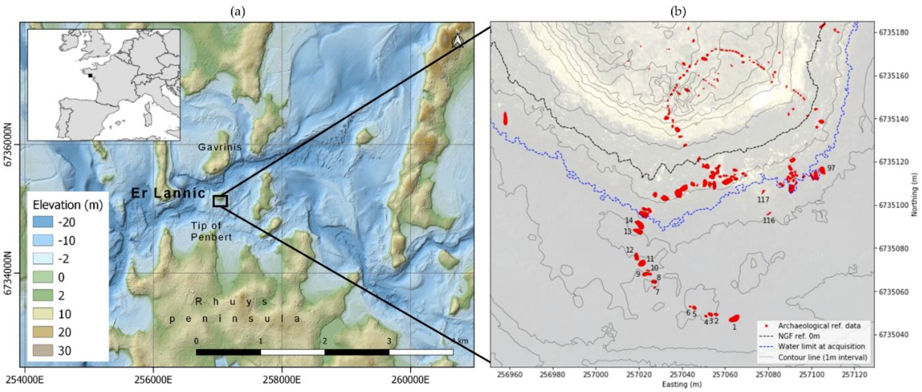
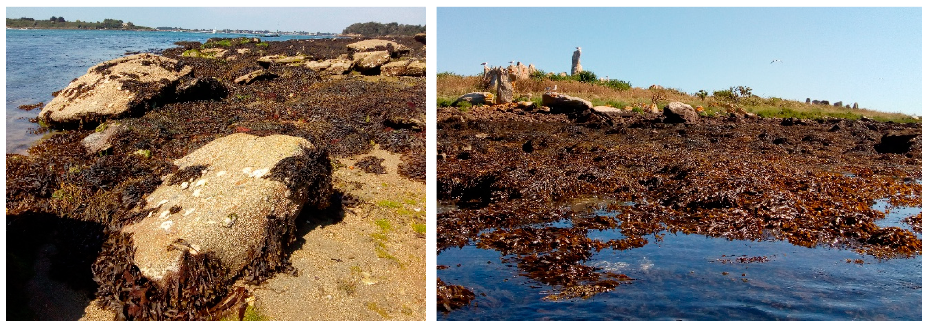
2.1. Study Area

The Gulf of Morbihan (France) has one of the most important architectural heritages of megaliths in the world. Due to their density and exceptional character, these Neolithic monuments, built from the 5th to 3rd millennia BC, are candidates for the UNESCO World Heritage List. One of the most emblematic sites in this region is the islet of Er Lannic and its two semicircular stone monuments.

The islet of Er Lannic, 80 ha in size, lies between the island of Gavrinis (with an imposing tumulus and abundant Neolithic engravings), 300 m to the north, and the Point of Penbert, on the Rhuys peninsula, 500 m to the south (Figure 1a). The islet borders the main channel of the Gulf of Morbihan, which has one of the strongest tidal currents in Europe.

The two semicircular stone monuments, each 50–60 m wide, are located on the southern end of Er Lannic. After its construction by Neolithic humans, the site was submerged due to the rise in sea level during the post-glacial marine transgression [32]. The coastline of the Gulf of Morbihan is estimated to have been ca. 5 m below the current sea level during the Neolithic period [32]. The megalithic site of Er Lannic (Figure 2) was first mentioned in 1866 by archaeologist G. de Closmadeuc [33]. Initially, only the terrestrial part of the monument was discovered and identified as a complete stone circle. The submerged structures were then revealed to archaeologists several years later by an extremely low tide. The first site map, depicting two adjacent stone circles, was drawn in 1882 [34]. Since then, several archaeological operations have been performed on site to complement and improve the site map. However, the strong tidal current and rock outcrops at the sea surface complicate surveys of the subtidal rocky platform, preventing any MBES surveys by boat. Despite the scientific interest of the site, few underwater measurements have been taken. The most recent documented underwater surveys were performed in the early 1990s [35] using traditional topographic techniques with a theodolite and a leveling rod, the latter being held in shallow water by divers during each measurement.

2.2. Airborne Hyperspectral Data

The study was based on AHI acquired by Hytech Imaging (Plouzané, France) with a NEO HySpex VNIR-1600 push broom sensor (

Table 1. Characteristics of the HySpex Visible Near Infra-Red (VNIR)-1600 sensor.

Spectral Range	Spatial Pixels	Spectral Resolution	Spectral Sampling	Number of Bands	FOV across Track	Pixel FOV across/Along Track	Coding
0.4–1.0 µm	1600	4.5 FWHM	3.7 nm	160	17°	0.18 mrad/0.36 mrad	12 bits

). The sensor was coupled with an IMAR iTrace-RT-F200 system and an OmniSTAR L1/L2 GNSS antenna to measure position and orientation.

The aerial survey was performed on 14 September 2018 at an altitude of ca. 1200 m to obtain a ground sampling distance of 50 cm (

Table 2. Parameters of the aerial survey.

Flight Altitude	Ground Sampling Distance	Swath	Integration Time	Viewing Angle	Solar Zenith Angle
1200 m	50 cm	176 m	10.1 ms	16.75°	16.75°

).

During the survey, images were collected in clear sky and calm sea conditions (preconditions to reduce sun-glint effects and solar irradiance variation). Er Lannic was overflown at 13:00 UTC, corresponding to low-tide conditions (tide coefficient of 85).

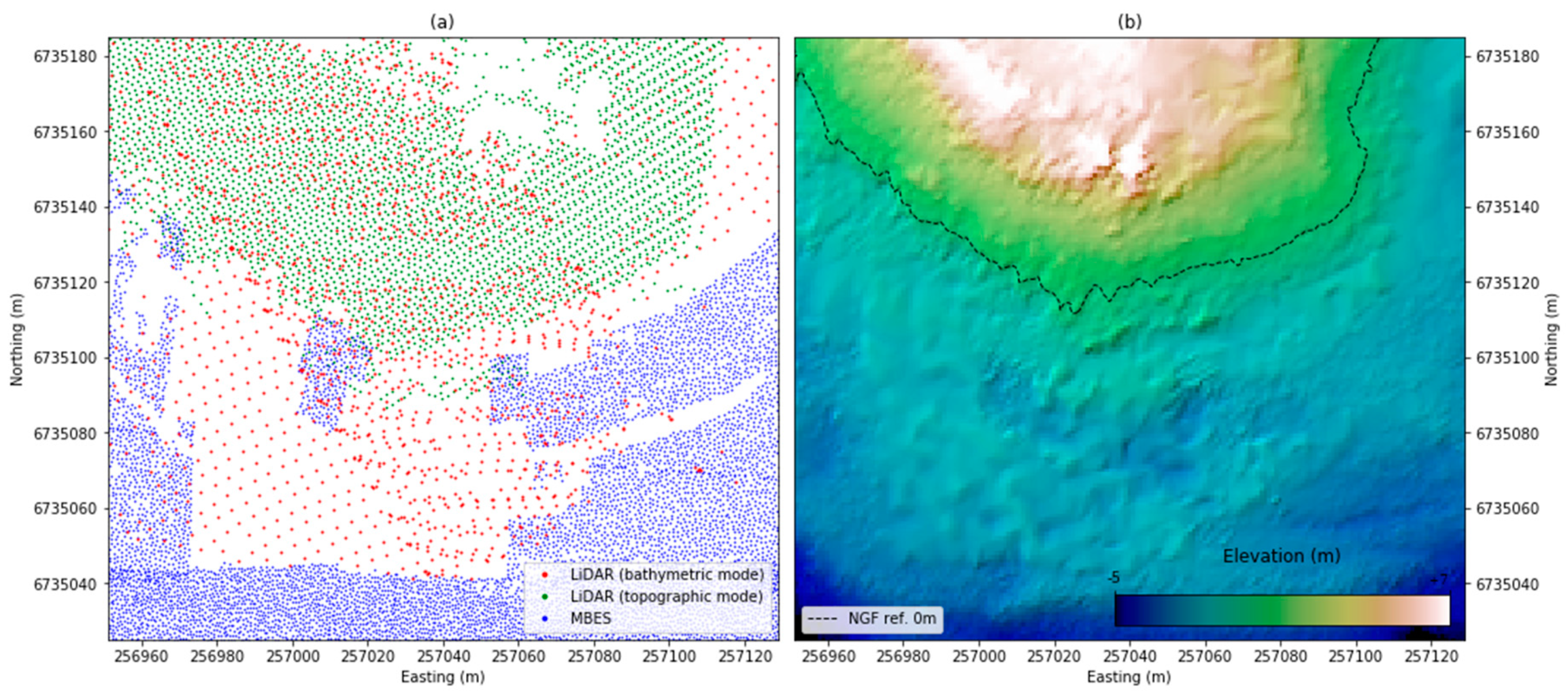
2.3. Bathymetric Reference Data

The reference bathymetric data used for this study are based on the Litto3D project [36,37] of the French Naval Hydrographic and Oceanographic Office (Shom) and the French National Geographic Institute (IGN). This project produced a seamless, high-resolution topographic and bathymetric model of French coastal areas using multiple survey techniques (Topographic LiDAR, ALB, MBES). For the Gulf of Morbihan, the Litto3D data consist of three complementary, locally overlapping surveys:

• ALB (SHOALS-1000T) by Shom (2005):

  ○

  Topographic and bathymetric modes: spot spacing 2 and 5 m, altitude 900 and 400 m, absolute planimetric accuracy < 1.5 and < 2.8 m, and absolute vertical accuracy < 0.3 and < 0.5 m, respectively

• MBES by Shom (2003) and IFREMER (2013)

Shom/IGN provided the data as a merged 3D point cloud with source identifiers (Figure 3a). Each point is defined as XYZ coordinates in Lambert93 system using the RGF93 geodetic system (EPSG: 2154) and NGF/IGN69 height reference for elevation. The merged point cloud was converted to a raster of 1 m resolution using Triangulated Irregular Networks interpolation (Figure 3b).

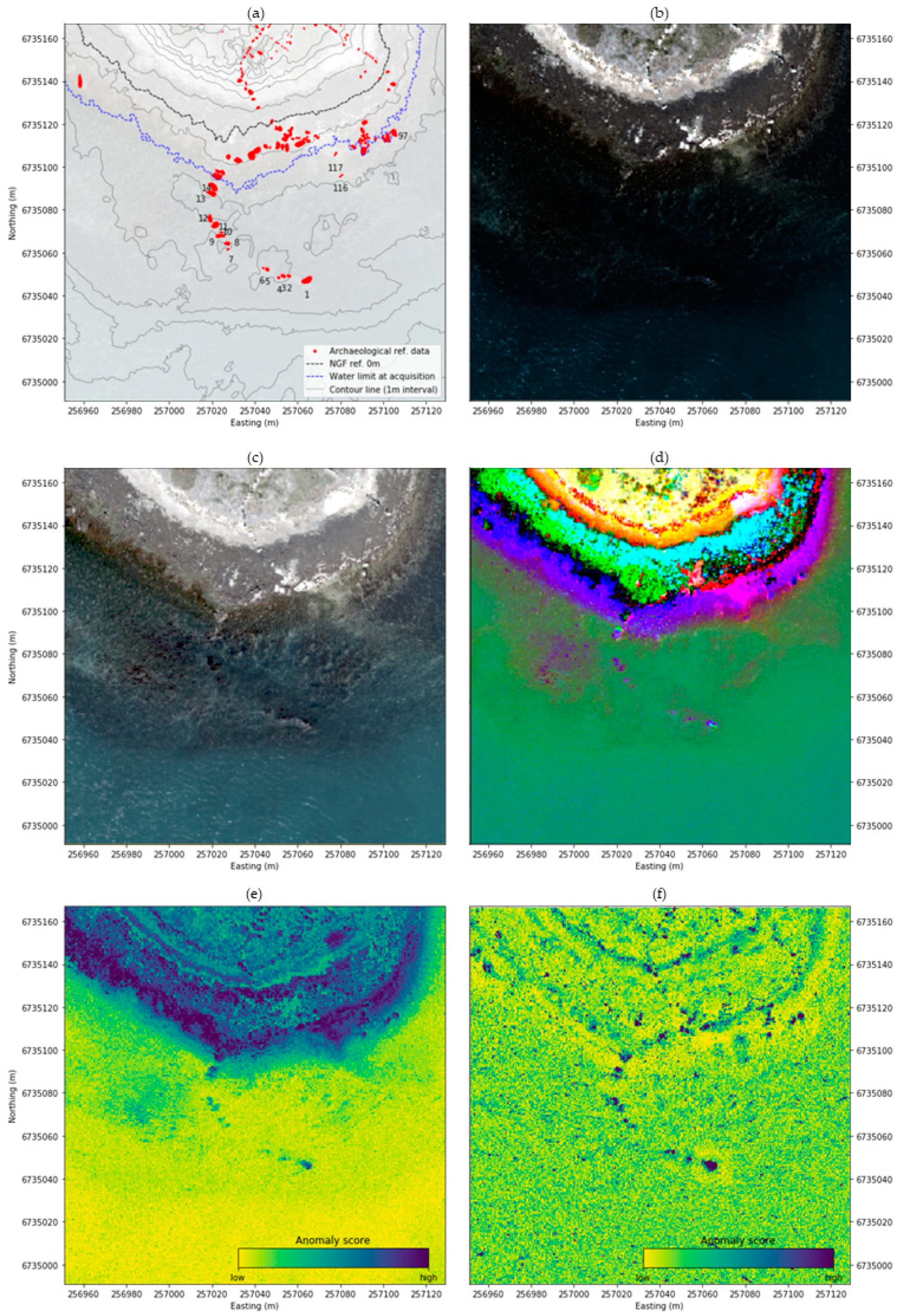
2.4. Archaeological Reference Data

Archaeological reference data for this study came from a georeferenced 2D map (Figure 1b) of each stone (or stele) of the site recorded by archaeologists from 1990-2018 [38,39,40]. The Regional Archaeological Service of Brittany (DRAC/SRA) currently uses this map. The map is projected in the Lambert93 system using the RGF93 geodetic system (EPSG: 2154).

Spatially, the northernmost semicircular stone monument, composed of ca. 60 steles—collapsed or erect—is entirely visible at lowest astronomical tide. The second semicircular stone monument, composed of 29 steles, is submerged and sits on the shore platform 2–3 m below mean sea level. Additional steles are also present at the junction of the semicircles, near a granite outcrop north of the second semicircle, and at isolated points away from the semicircles. The steles, most of them metamorphic orthogneiss, vary in projected horizontal area from < 0.5–11 m².

For identification purposes, steles are numbered from 1-201 [38] (i.e., $St{l}_{\#1}$ to $St{l}_{\#201}$). Based on the tide and sea conditions when the images were acquired, 17 steles ($St{l}_{\#1}$ to $St{l}_{\#14}$, $St{l}_{\#97}$, $St{l}_{\#116}$ and $St{l}_{\#117}$) were located beyond the shoreline, of which 15 were completely submerged and 2 ($St{l}_{\#1}$ and $St{l}_{\#14})$ were partially submerged.

2.5. Dimensionality Reduction and Visualization

Dimensionality reduction techniques concentrate information by projecting the original data, with high dimensionality, into a lower dimensional space. Its objective is to decrease computational burden (i.e., reduce the number of bands), remove spectrally redundant information or noise and highlight informative spectral variation in the imagery. For remote-sensing hyperspectral data, for which interband correlation is high and noise omnipresent, dimensionality reduction algorithms are used to enhance visual interpretation or as pre-processing before other procedures, such as classification [30]. These algorithms include Principal Component Analysis (PCA) and Minimum Noise Fraction (MNF) [41]. PCA projects data into a new subspace where the projected components maximize the variance of the data under the constraint that each component is orthogonal to its preceding component. PCA can thus reduce dimensionality of the data while conserving the maximum amount of information. When applied to hyperspectral imagery, however, PCA is not the most suitable method, notably because of its limitation with noisy observations. MNF is a linear transformation based on two sequential PCA rotations. The first rotation decorrelates and scales the noise using a noise covariance matrix calculated by estimating local noise using the difference between adjacent pixels. The result is a hyperspectral data cube in which noise has unit variance and no band-to-band correlation (white noise). The second rotation performs a PCA on the noise-whitened data cube to separate noise from data and thus maximize the signal-to-noise ratio (SNR).

2.6. Unsupervised Anomaly Detection

In the machine learning field, unsupervised learning is the task of identifying structures or relationships in the input data without prior knowledge by mean of reference or labelled data. Since submerged archaeological structures might be undescribed in nature, degraded or covered (with sediments, vegetation or biofilm), archaeological prospection using remote-sensing data usually seeks anomalies rather than looking for known signatures [24,31]. Unsupervised anomaly-detection techniques are adapted to these conditions, since they require no predefined target characteristics and try to separate common observations from unusual observations. Doing the latter requires two main assumptions: anomalies are (i) spectrally different from the surrounding background and (2) represent a minority of pixels in an image (low occurrence). Existing unsupervised anomaly-detection algorithms include the Reed–Xiaoli detector (RXD) and associated variants, and the Isolation Forest (IF) algorithm.

RXD, developed by [42], is based on a statistical distance (Mahalanobis distance) calculated between the observation (a pixel) and the image background. Global RXD relies on a pre-calculated background at the image level, while local RXD (LRXD) is based on a local background estimated using a sliding window that can have inner and outer sizes to adapt to specific anomaly sizes.

IF, developed by [43], is based on the widely used Random Forest classification algorithm. IF combines multiple weak decision trees to calculate an anomaly score that reflects how much an observation differs from other observations. Each tree is created recursively by randomly selecting a feature and an associated random threshold value. Each observation is passed through the tree and compared to each node (feature and threshold) until it can be isolated from other observations (reaching an external node). The shorter an observation’s path in the tree, the higher is its anomaly score. The final anomaly score equals the mean score of all trees.

2.7. Radiative Transfer Model over Shallow Water

Over optically shallow water (inland or coastal waters whose bottom is visible from the surface), total radiance measured by the remote sensor includes contributions from the atmosphere, the water surface, the water column and the water bottom. Hyperspectral remote sensing uses this radiative relationship to characterize the water column and water bottom physically. The radiative transfer model of Lee [44] calculates subsurface remote-sensing reflectance $R_{rs}^{-}$ as:

$$R_{rs}^{-}=R_{rs}^{\infty }\left(1-A_1{e}^{-\left(K_d+k_{uW}\right)Z}\right)+A_2{R}_{rs}^B{e}^{-\left(K_d+k_{uB}\right)Z}$$

(1)

where $R_{rs}^{\infty }$ is the remote-sensing reflectance for optically deep water; $K_d$, $k_{uW}$, $k_{uB}$ are diffuse coefficients related to downwelling irradiance, upwelling radiance of the water column, and upwelling radiance from bottom reflection, respectively; $A_1$ and $A_2$ are constants; $R_{rs}^B$ is the bottom reflectance and $Z$ is the bottom depth.

Equation (1) verifies that for $Z\to \infty$, $R_{rs}^{-}\to R_{rs}^{\infty }$, and for $Z\to 0$, $R_{rs}^{-}\to R_{rs}^B$. This semi-analytical model is then inversed to retrieve the parameters (including $R_{rs}^B$ and $Z$) that minimize the difference between the observed and modeled spectra [45].

This radiative-transfer–based method, unlike empirical approaches, has the advantage of not requiring prior bathymetric data (existing elevation model or in-situ measurements) for the inversion process and derivation of bottom depth [21].

3. Methodology

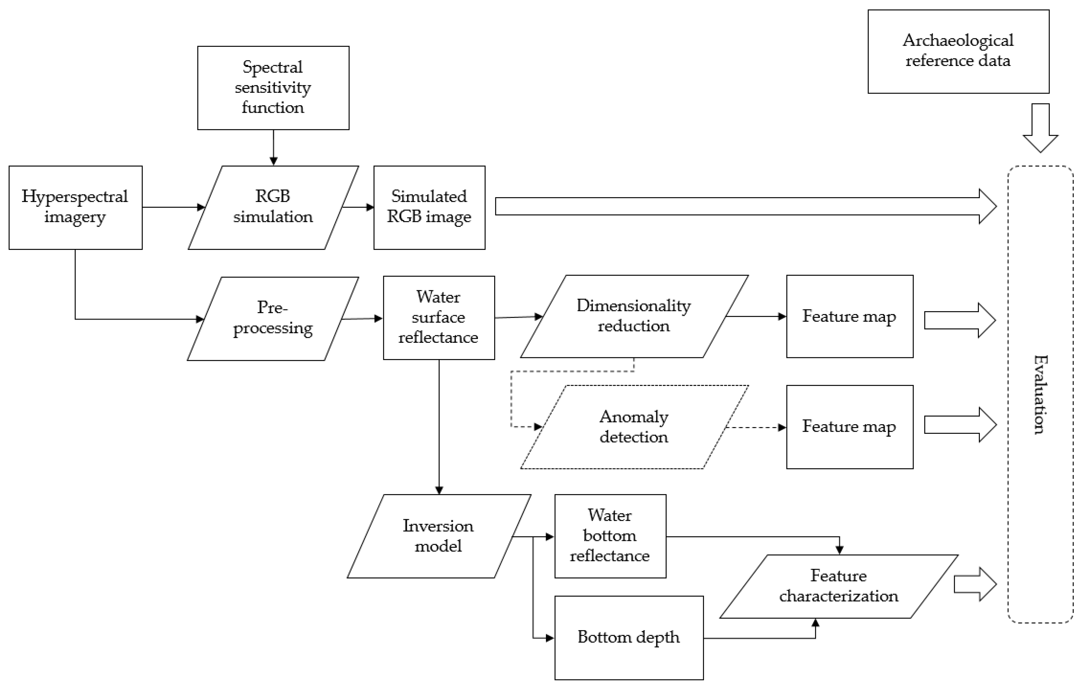
3.1. Workflow

The methodology developed and the associated workflow (Figure 4) were organized in subsections corresponding to the research questions of this study.

3.2. Pre-processing

The hyperspectral images were processed from level 0 (raw) to level1b (radiometrically and geometrically calibrated) using the HYPIP (HYPperspectral Image Preprocessing) chain of Hytech-imaging that includes ATCOR/PARGE software applications (ReSe Applications, Wil, Switzerland) to obtain georeferenced images in spectral radiance ($W.m^{-2}.s{r}^{-1}.\mu m^{-1})$. Surface reflectance was then obtained by performing atmospheric corrections in a two-step process: (i) atmospheric corrections using ATCOR-4 software and (ii) empirical adjustment of each spectrum by applying coefficients (gain and bias) calculated per spectral band by linear regression between surface reflectance data and the reflectance signature of pre-calibrated targets (tarps) positioned near the area of interest and overflown during the survey. The resulting hyperspectral products (at-sensor radiance, surface reflectance) were then spatially subset to a 2048 px × 2048 px tile (representing an area of ca. 1 km²), encompassing the area of interest of Er Lannic islet.

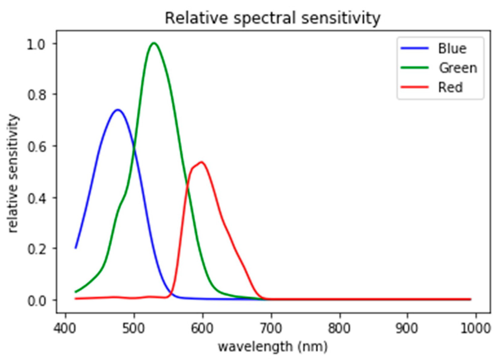
3.3. Simulation of True-color Image

The initial hypothesis of the study was that VNIR AHI carries information valuable for visualizing submerged archaeological structures. To evaluate the contribution of hyperspectral data compared to that of traditional true-color photography, a red-green-blue (RGB) image was simulated using the spectra sensitivity response (Figure 5) of a digital single-lens reflex camera (DSLR Canon EOS 10D) and the hyperspectral cube.

Red, green and blue bands of the simulated image were produced by convolution products (Equations (2), (3) and (4), respectively):

$$Re{d}_{sim}={\displaystyle \sum }_{\mathsf{\lambda }400}^{\mathsf{\lambda }700}RS{S}_r\left(\mathsf{\lambda }\right)\ast L{\left(\mathsf{\lambda }\right)}_{tot.}^s$$

(2)

$$Gree{n}_{sim}={\displaystyle \sum }_{\mathsf{\lambda }400}^{\mathsf{\lambda }700}RS{S}_g\left(\mathsf{\lambda }\right)\ast L{\left(\mathsf{\lambda }\right)}_{tot.}^s$$

(3)

$$Blu{e}_{sim}={\displaystyle \sum }_{\mathsf{\lambda }400}^{\mathsf{\lambda }700}RS{S}_b\left(\mathsf{\lambda }\right)\ast L{\left(\mathsf{\lambda }\right)}_{tot.}^s$$

(4)

where $L{\left(\mathsf{\lambda }\right)}_{tot.}^s$ is the at-sensor radiance from hyperspectral imagery, and $RS{S}_r\left(\mathsf{\lambda }\right),RS{S}_g\left(\mathsf{\lambda }\right),andRS{S}_b\left(\mathsf{\lambda }\right)$ are relative spectral sensitivity functions of the red, green and blue channel, respectively, of the DSLR ([46] citing [47]).

The contrast/brightness of the simulated RGB image was then adjusted using gamma correction (γ = 0.4) to improve visualization [48].

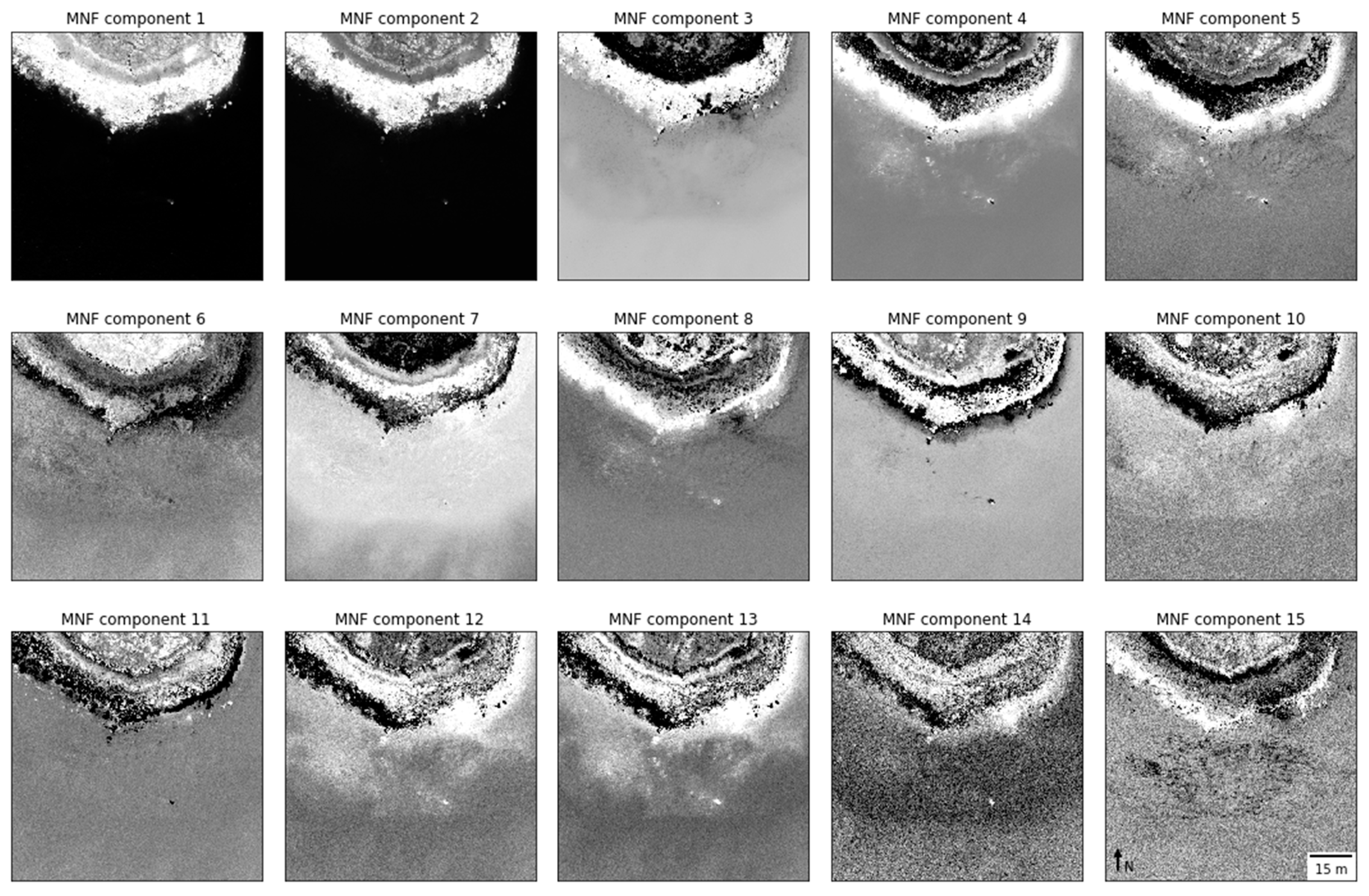
3.4. Dimensionality Reduction Using MNFMinimum Noise Fraction Transform

MNF transform was then applied to the reflectance hyperspectral images. Full spectral information from 400–1000 nm wavelengths was kept for the MNF decomposition. Noise was estimated by (i) selecting a homogeneously dark area of the image and (ii) extracting the noise covariance matrix from it using the shift difference method (i.e., the processed pixel minus its top-right neighbor). This procedure respectively exploits the facts that (i) signal variation in a homogeneously dark area of an image is due primarily to environmental and instrumental noise and (ii) the signal at any point in the image is strongly correlated with the signal at neighboring pixels, while noise is not or only weakly spatially correlated [41].

Given the site context and to allow for continuous visual interpretation of terrestrial and submerged structures (including rock outcrops or emerging steles), the MNF transform was applied to the entire subset of the imagery, including terrestrial and submerged areas. Only MNF components with a SNR ≥ 5 were conserved. The resulting components were visualized individually and in multiple pseudo-colored images (combining three components selected to highlight spectral and spatial variation in the data) to enhance visualization of submerged features. The results were compared to (i) the synthetically created true-color image and (ii) the georeferenced archaeological reference data identifying each stele.

3.5. Automatic Anomaly Detection

LRXD and IF unsupervised anomaly-detection algorithms were used to identify submerged anomalies automatically and compare them to the known archaeological reference data. The algorithms were applied to the MNF results calculated from the surface reflectance image. LRXD was applied to the MNF subset within a sliding window of 30 px × 30 px (outer window) and 15 px × 15 px (inner window). The IF model was trained with 100 decision trees, 100 randomly drawn observations and 10 randomly drawn features to train each tree.

For both algorithms, results were evaluated visually and statistically. Visually, the anomaly score map was compared to the georeferenced archaeological reference data. Statistically, the receiver operating characteristic (ROC) curve was calculated to illustrate the trade-off between the true positive rate and false positive rate at different score thresholds. Accuracy was assessed by calculating a normalized confusion matrix of the binary classification with a threshold defined from the ROC curve. Statistical evaluation was limited to the submerged area to focus on submerged anomalies.

3.6. Depth and Bottom Reflectance Estimation

Before inverting the radiative transfer model, a mask for the water was applied using the normalized difference water index (NDWI) [49]:

$$NDWI=\frac{R\left({\lambda }_{550}\right)+R\left({\lambda }_{850}\right)}{R\left({\lambda }_{550}\right)-R\left({\lambda }_{850}\right)}$$

(5)

where $R\left({\lambda }_{550}\right)$ and $R\left({\lambda }_{850}\right)$ are the pixel reflectance values in the green and near-infrared areas of the spectrum, respectively.

To reduce variability due to noise, reflectance was extracted using the median values within ± 20 nm of each central wavelength (550 or 850 nm).

The semi-analytical radiative-transfer model, as seen in Equation (1) was inverted using SWIM (Shallow Water mappIng using optical reMote sensor(s)) [45,50] to estimate bottom reflectance ($R_{rs}^b)$, bottom depth ($Z)$ and water column parameters ($C_{cdom},C_{phy},C_{NAP}$) from the observed subsurface reflectance $(R_{rs}^{-}$). The inversion problem is solved by minimizing a least square cost function representing distance between the observed subsurface reflectance and the modelled subsurface reflectance. Optimization was performed using the Levenberg-Marquardt. For each pixel, the algorithm converged to a solution for a vector of parameters ($R_{rs}^b,Z,C_{cdom},C_{phy},C_{NAP}$). $R_{rs}^b$ and $Z$ were used subsequently for further analysis. No external data (in-situ depth measurements or existing elevation model) was used for refining the bottom-depth estimation.

The bottom depth in raster format was post-processed using a median filter of 5 × 5 px to reduce the salt-and-pepper noise that can decrease interpretability for archaeological purposes. The data were then corrected for the tidal effect using tide information available from Shom and converted from the hydrographic reference to the terrestrial height reference NGF/IGN69 using the RAM product (maritime altimetric reference values) provided by Shom. The results were compared to the archaeological reference data as well as to the Litto3D continuous topo-bathymetric reference dataset collected from MBES and ALB by Shom/IGN on the Gulf or Morbihan.

4. Results

4.1. Analysis of the Simulated Rgb Image

The northernmost and terrestrial semicircle of Er Lannic was visible on the RGB image, as were the locations of archaeological structures (individually for large steles and linear shapes for groups of smaller steles) (Figure 6b,c). Bright colors of on-shore steles and shadows projected by standing steles facilitated visualization and interpretation. On the submerged part of the site, large terrestrial steles on the upper intertidal platform were apparent, but the continuity of the submerged semicircle was difficult to perceive without prior knowledge of the site or the reference archaeological data. Effects of the water surface were visible at the southern tip of the semicircle and corresponded to the presence of an emerging stele ($St{l}_{\#1}$).

4.2. Analysis of the Hyperspectral Imagery

According to the MNF components extracted from AHI, the hyperspectral data did not greatly improve visualization or description of the northernmost semicircle (Figure 7). However, the variability in the ground spectral signature near the steles highlighted many natural ground features (e.g., sands, granitic rocks, dry algae, grass). On intertidal and submerged platforms, the presence of features (local variations in MNF) through the water-column was visually confirmed, especially from MNF components 3, 4, 5, 8, 9, 12 and 13. Local variations were visually interpreted to identify the presence of the submerged semicircle.

The pseudo-color image, created from visual selection of components 3 (green), 4 (blue) and 9 (red) of the MNF, confirmed the identification of submerged anomalies corresponding to the submerged steles ($St{l}_{\#1}$ to $St{l}_{\#14}$, $St{l}_{\#97}$, $St{l}_{\#116}$ and $St{l}_{\#117}$) (Figure 6d).

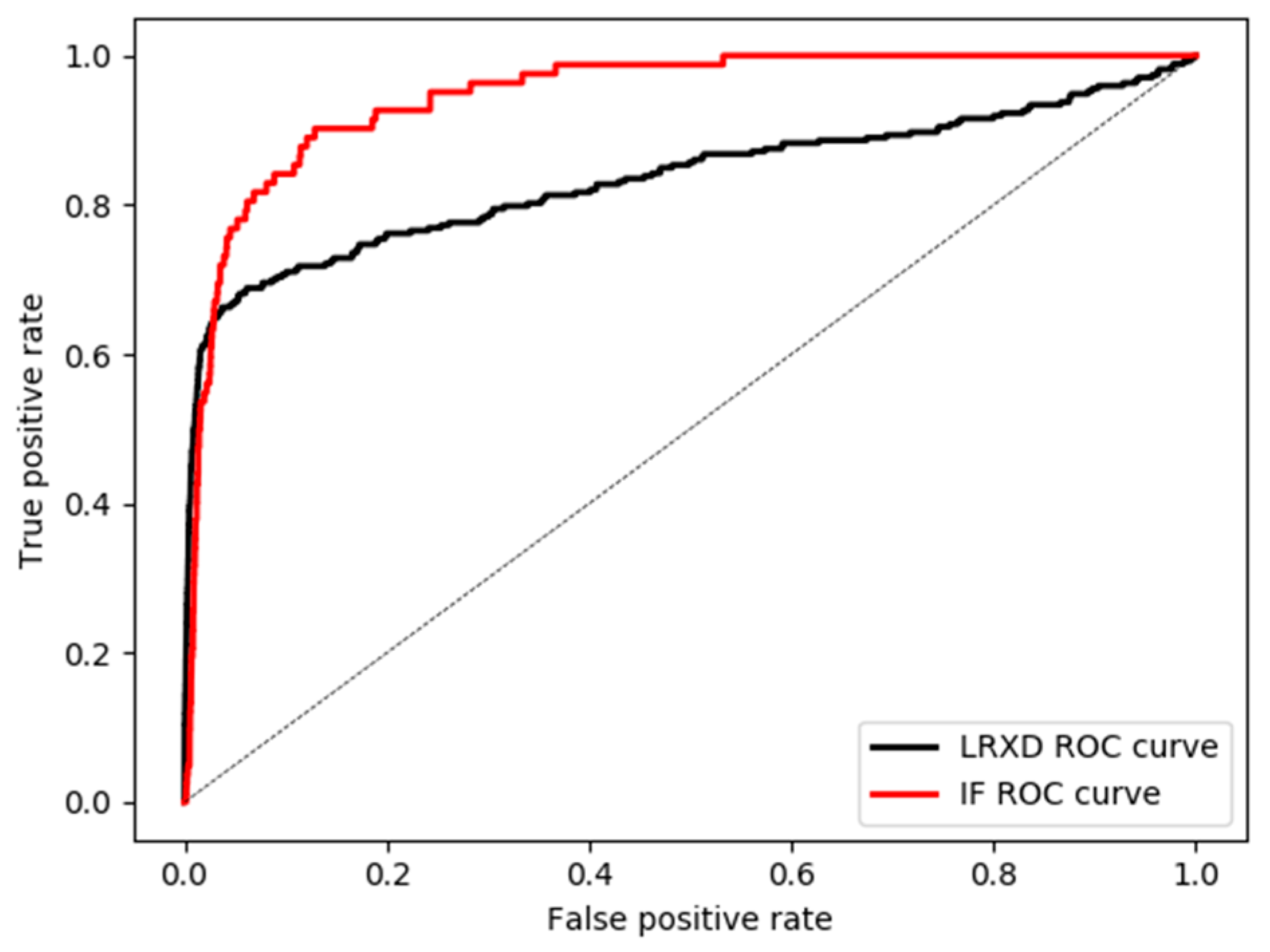
4.3. Automatic Detection of Archeological Structures

According to IF, the most anomalous pixels were located mainly on-shore due to the high variability in spectral signatures (Figure 6e). Submerged archaeological structures had lower scores (i.e., less anomalous than on-shore structures) but were clearly visible and spatially defined due to their difference with the background (common observations). In contrast, structures at the land/water interface were not clearly defined due to little difference in the anomaly score.

Results obtained with the LRXD algorithm emphasized the location and shape of each submerged structure (Figure 6f). While LRXD is subject to impulse noise due to anomalous single-pixel observations, the spatial pattern of the submerged monuments was clearly distinguishable as a whole and as individual steles.

Comparing statistical results of the submerged area (at the time of acquisition) of the IF and LRXD methods, IF performed better than LRXD because LRXD (i) tended to enlarge anomalies spatially and (ii) generated a higher false positive rate (0.16, vs. 0.08 for IF) because it detected more anomalies on the submerged area (

Table 3. Normalized confusion matrix for Isolation Forest (IF) and local Reed–Xiaoli detector (LRXD) anomaly detection of submerged structures.

	Predicted Label “Standard”	Predicted Label “Anomaly”
True label “standard”	0.92 (IF) 0.84 (LRXD)	0.08 (IF) 0.16 (LRXD)
True label ”anomaly”	0.12 (IF) 0.27 (LRXD)	0.88 (IF) 0.73 (LRXD)

, Figure 8).

4.4. Characterization of Archeological Structures

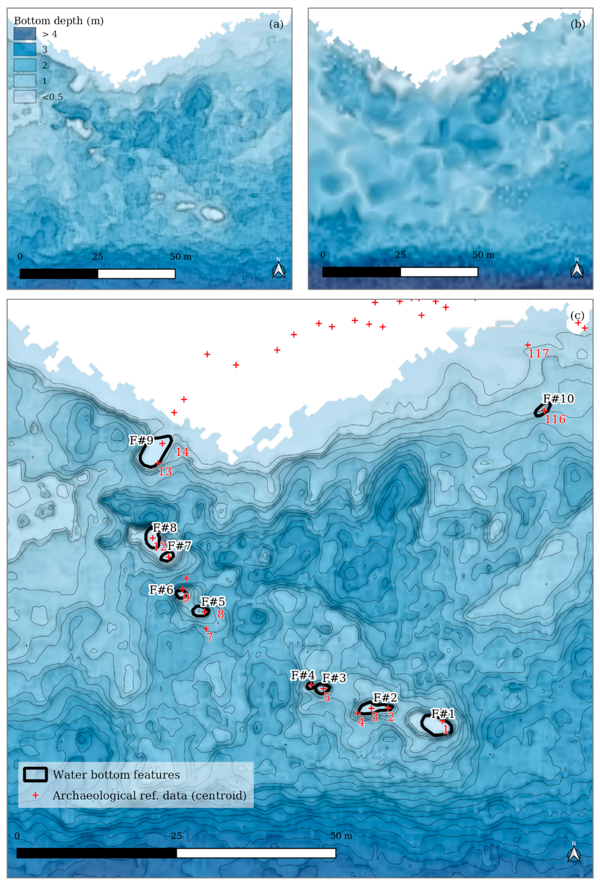
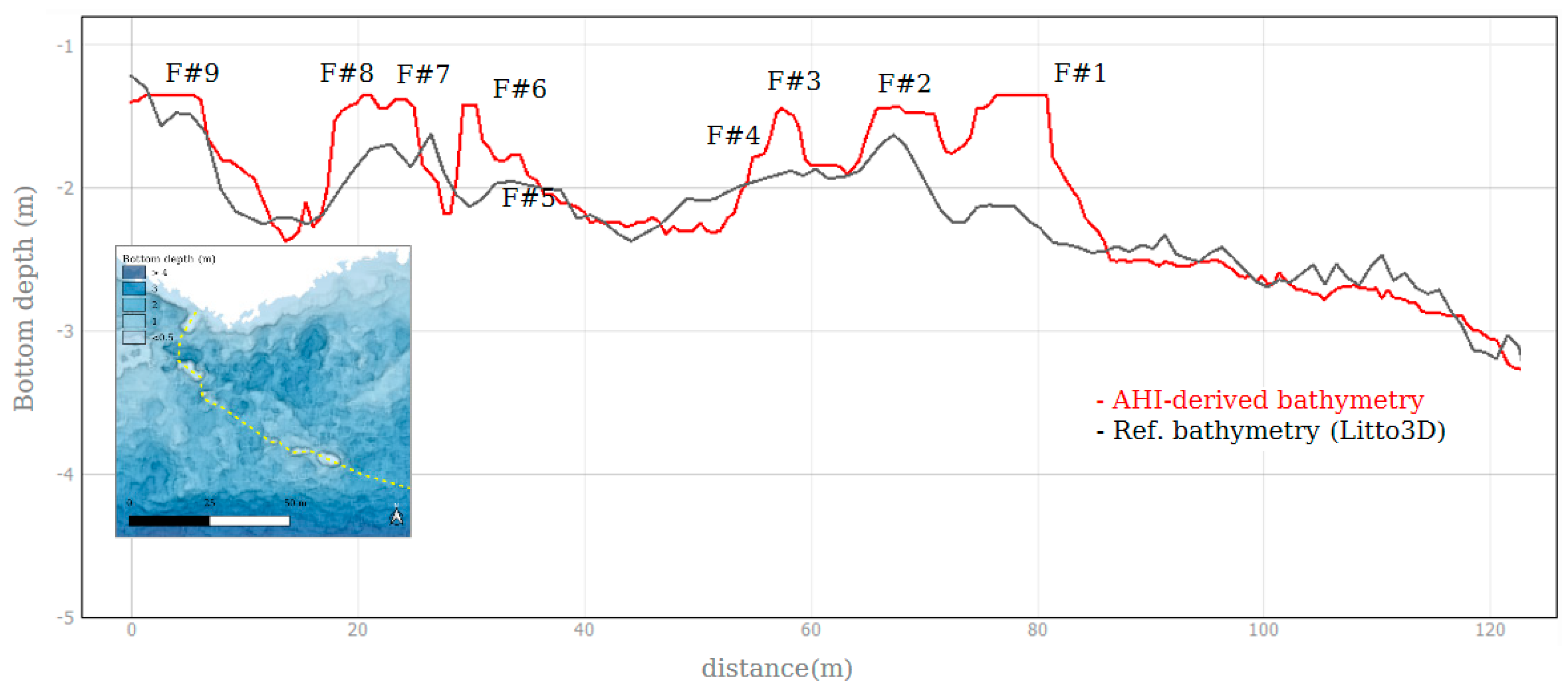
4.4.1. Morphological Characterization

The Bathymetric Digital Elevation Model (DEM) derived from AHI showed topographic variations corresponding to the submerged steles. An adapted view (using slope and colored-ramp overlay blending and 0.1 m contour lines) of the estimated water bottom highlighted the features (local maxima) and provided an initial morphological description (shape, area). On the submerged semicircle, 10 features on the DEM were interpreted as archaeological structures (Figure 9). Eight of these features (denoted F#) were associated with single steles (F#1: $St{l}_{\#1}$, F#3: $St{l}_{\#5}$, F#4: $St{l}_{\#6}$, F#5: $St{l}_{\#8}$, F#6: $St{l}_{\#9}$, F#7: $St{l}_{\#11}$, F#8: $St{l}_{\#12}$, F#10: $St{l}_{\#116}$), while the other two were associated with aggregations of multiple steles (F#2: $St{l}_{\#2}$, $St{l}_{\#3}$, $St{l}_{\#4}$; F#9: $St{l}_{\#13}$, $St{l}_{\#14}$) since individual DEM signals for them were not apparent. Submerged steles $St{l}_{\#7}$, $St{l}_{\#10}$ and $St{l}_{\#117}$ were not identified from the AHI-derived water-bottom morphology.

The area of the features extracted (2D projected horizontal area) were then compared to those of the archaeological reference data (

Table 4. Area of airborne hyperspectral imagery-derived water-bottom features compared those of steles from archaeological reference data. Coefficient of determination R² = 0.72.

Feature ID $\left(\mathit{F}\mathit{e}\mathit{a}{\mathit{t}}_{\#\mathit{n}}\right)$	Feature Area (m2)	Stele IDs $\left(\mathit{S}\mathit{t}{\mathit{l}}_{\#\mathit{n}}\right)$	Stele Area (m2)
1	10.3	$St{l}_{\#1}$	9.8
2	5.8	$St{l}_{\#2}$, $St{l}_{\#3}$, $St{l}_{\#4}$	4.7 (1.4, 2.4, 0.9)
3	2.5	$St{l}_{\#5}$	2.1
4	0.7	$St{l}_{\#6}$	0.5
5	4.0	$St{l}_{\#8}$	9.0
6	1.5	$St{l}_{\#9}$	4.8
7	2.0	$St{l}_{\#11}$	6.9
8	5.1	$St{l}_{\#12}$	4.7
9	15.1	$St{l}_{\#13},St{l}_{\#14}$	16.1 (6.9, 9.2)
10	2.8	$St{l}_{\#116}$	0.7

). Linear regression between the two indicated relatively good agreement (R² = 0.72).

Visualization of a path profile of bottom depth along the submerged semicircle (Figure 10) allowed AHI-derived bathymetry and Litto3D reference bathymetry to be compared. AHI-derived bathymetry described water-bottom morphology in more detail, and the presence of local maxima at the location of known archaeological structures confirmed its ability to visualize submerged structures and, to some extent, describe their morphological characteristics (i.e., shape, depth, and area).

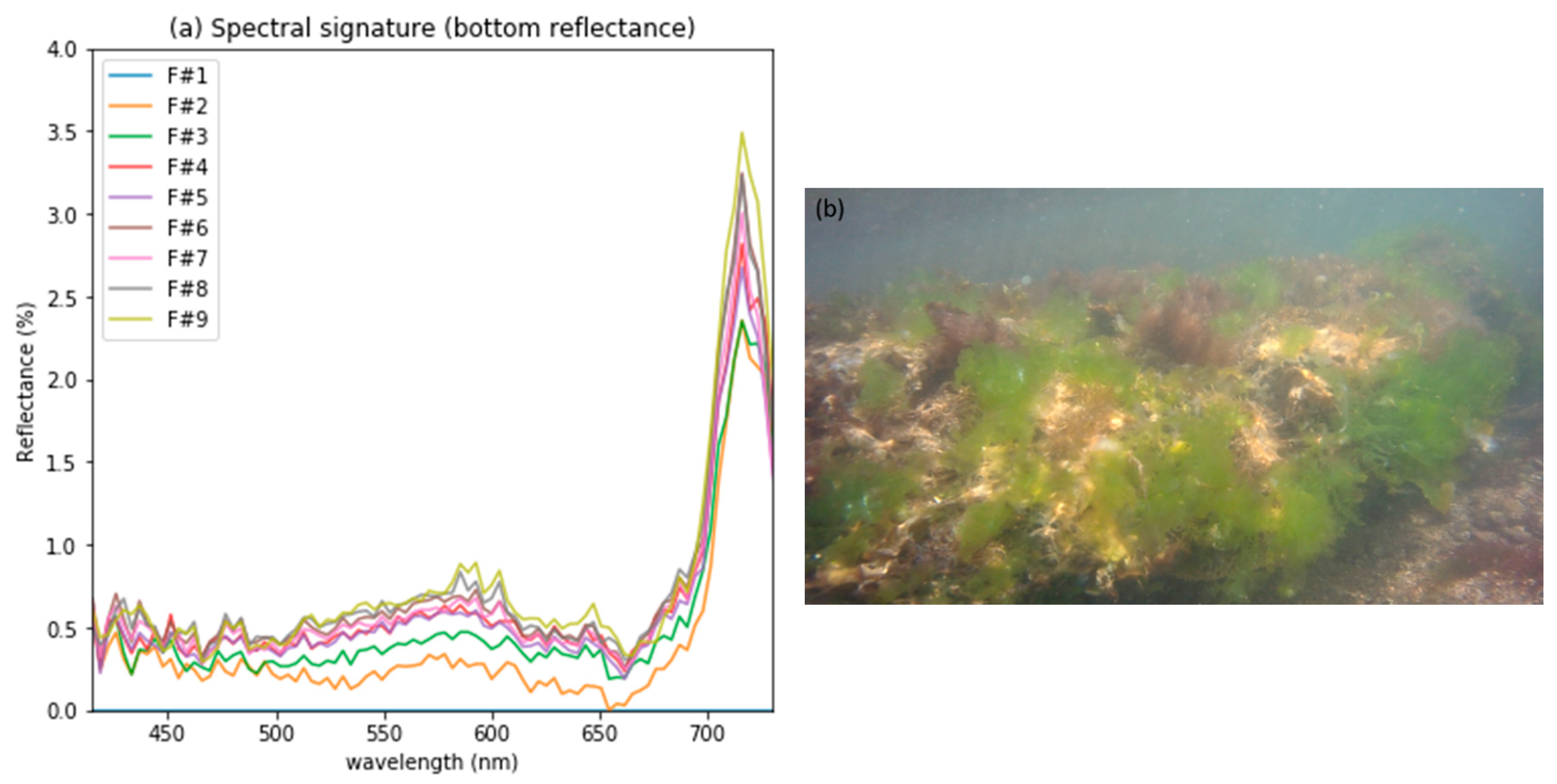
4.4.2. Spectral Characterization of the Archeological Structures

Spectral signatures (bottom reflectance) selected on the submerged semicircle (Figure 11a) had a low amplitude of estimated reflectance (< 1%) due to low reflectivity of the water bottom. It also revealed green (around 580nm) and red-edge (increase in spectral reflectance from 650–720 nm) peaks on the submerged features, which reflected the presence of vegetation in plant-based biofilm (i.e., micro-algae) or macro-algae on the steles. In-situ observations (Figure 11b) confirmed the presence and the diversity of macro-algae (green and brown) on the steles.

5. Discussion and Perspectives

5.1. AHI: Potential for Application to Underwater Archaeology

Until recently, ALB was considered the only aerial remote-sensing technique that could collect high-resolution data in very shallow water [51]. Development of AHI for shallow water mapping, first in academic contexts and more recently towards operational usages, shows that passive remote sensing is becoming a potential alternative for estimating bathymetry and describing water-bottom morphology and benthic cover types at a fine scale (meter or sub-meter resolution) [21,52]. The present study opens new perspectives for underwater cultural heritage monitoring and archaeological prospection. Benefits of AHI for these applications include lower survey costs than those of ALB [53] and high spectral and spatial description. However, AHI also has drawbacks. As AHI is an optical remote sensing system (such as ALB), the efficiency of AHI for accessing water bottom information depends on environmental factors such as turbidity, water surface condition and sea state, bottom depth and bottom reflectance. Moreover, as a passive optical system, the quality of the data is also dependent on the illumination conditions and cloud cover [54]. While additional investigations are required to determine the dependency of the proposed approach on these environmental variables, the management of AHI surveys for archaeological mapping in a shallow water environment remains a sensitive aspect of the workflow.

5.2. Data Uncertainty and Statistical Results

The statistical results for unsupervised detection of anomalies were influenced by uncertainties in the context and input data. Since the target structures we sought had areas of 0.5–10 m², they were represented by clusters of a few pixels in the image (spatial resolution: 50 cm). Given this resolution, the sensor’s point spread function and the uncertainty in horizontal precision (usually 1-2 pixels), the probability of having local/spatial discrepancies between the collected data and the reference data was relatively high. Another source of uncertainty was the reference archaeological data. Like for other archaeological reference data, a “ground truth” map is limited by at least two factors. The first is the measurement itself: every spatial measurement is inaccurate (as it never exactly matches with the true value which remains undefined), especially for archaeological sites of limited accessibility (i.e., partially or entirely submerged), and the uncertainty in location can be high. The second is the exhaustiveness of the reference data, which is never guaranteed. Since the reference map of an archaeological site evolves with methods and techniques, it should be considered a “current state of knowledge” rather than a “ground truth”. Since we did not consider any of these sources of uncertainty, the results must be analyzed with care. They should not be considered a baseline for similar approaches in different archaeological contexts, but rather a baseline for comparing novel anomaly-detection methods in the same experimental conditions.

5.3. From Anomaly to Archaeological Structure

As shown in this study, morphological and spectral characterization of submerged archaeological structures can be complex. The weak reflectance (and consequently low SNR) in water conditions, combined with the continuous presence of vegetation (micro- or macro-algae) on submerged mineral structures, limited the ability to distinguish between archaeological and natural structures spectrally. Thus, the use of the term "morphological or spectral characterization" could be an inappropriate description of hyperspectral remote sensing if it is assumed to provide information similar to that from in-situ archaeological analysis. Considering the information provided by remote sensing to be a faithful description of archaeological structures is premature. Instead, the information provided by AHI should be considered a proxy or surrogate description of archaeological structures. For example, archaeologists consider that algae covering steles are not part of the archaeological structures (in fact, algae are regularly removed from the steles of Er Lannic that are accessible at low tide). Therefore, the morphological or spectral descriptors of submerged features extracted from remote sensing data describe not only archaeological structures but the natural environment that surrounds them (their envelope). Nevertheless, a first characterization of the bottom spectral properties is a valuable information offered by AHI and an advantage over ALB for which the backscattering intensity of a single wavelength signal is less adapted for the description of benthic composition [55].

5.4. Perspectives and Future Research Directions

This study was an initial approach to demonstrate the potential of hyperspectral imagery for prospecting and monitoring submerged archaeological structures in shallow water environments. It opens new perspectives. First, from an archaeological perspective, the study focused on a known archaeological site built during the Neolithic period. The archaeological potential in coastal shallow water environment, for example in Brittany, is important and a major challenge from a scientific perspective and with regard to cultural heritage management. Our objective is to broaden this study to prospect or monitor archaeological sites of different chrono-typologies.

Second, from a remote-sensing and data-analysis perspective, we intend to continue research on unsupervised and supervised anomaly detection. For archaeological prospection, anomaly detection is a key challenge for identifying structures for which only partial knowledge usually exists. Indeed, the state of conservation and surface condition of archaeological structures, especially in water conditions, is a priori undefined, and the expected characteristics that reference typologies provide, although informative, can mislead prospections for predefined morphological structures that differ from the complex in-situ situation. To address this limitation, our future research will aim to go further in the use of unsupervised or self-supervised anomaly detection algorithms, including deep-learning techniques such as convolutional autoencoders in 2D (spatial) or 3D (spatial/spectral), to extract informative patterns from the hyperspectral cube for application to archaeology.

6. Conclusions

We demonstrated AHI’s potential for submerged archaeological prospection and monitoring in shallow water environments. While AHI is regularly used for terrestrial archaeology, its use has not yet been assessed for underwater archaeology. By taking advantage of the high-resolution spatial and spectral characteristics of AHI data, the study showed that AHI passive remote-sensing could be a valuable alternative to active remote-sensing techniques for mapping submerged archaeological structures. The study was performed on the megalithic site of Er Lannic in Morbihan (France), composed of two semicircles of steles, one of which lay on the water bottom 2–3 m below the mean sea level. The method was divided into three steps: (i) visualize submerged structures, (ii) detect submerged anomalies automatically and (iii) characterize the features identified by estimating their morphological and spectral characteristics. The results showed that hyperspectral data can collect underwater information necessary for archaeological mapping. This information was extracted from AHI either by data-driven analysis (dimensionality reduction/anomaly detection) or by estimating physical parameters such as water depth and bottom reflectance by the inversion of a radiative transfer model. Comparing the information extracted to archaeological and bathymetric reference data confirmed AHI’s potential for archaeological prospection and monitoring. Although this study focused on a single archaeological site (i.e., chrono-typology), the approach will be further explored to assess its application to a wider range of structures and archaeological and environmental contexts. Future research will also assess unsupervised or self-supervised machine-learning techniques to reduce dimensionality and detect submerged anomalies in hyperspectral images.

References

- Daire, M.-Y.; López-Romero, E.; Proust, J.-N.; Regnauld, H.; Pian, S.; Shi, B. Coastal Changes and Cultural Heritage (1): Assessment of the Vulnerability of the Coastal Heritage in Western France. J. Isl. Coast. Archaeol. 2012, 7, 168–182. [Google Scholar] [CrossRef]
- Reeder-Myers, L.A. Cultural Heritage at Risk in the Twenty-First Century: A Vulnerability Assessment of Coastal Archaeological Sites in the United States. J. Isl. Coast. Archaeol. 2015, 10, 436–445. [Google Scholar] [CrossRef]
- Singh, H.; Adams, J.; Mindell, D.; Foley, B. Imaging Underwater for Archaeology. J. Field Archaeol. 2000, 27, 319–328. [Google Scholar]
- Guzinski, R.; Spondylis, E.; Michalis, M.; Tusa, S.; Brancato, G.; Minno, L.; Hansen, L.B. Exploring the Utility of Bathymetry Maps Derived with Multispectral Satellite Observations in the Field of Underwater Archaeology. Open Archaeol. 2016, 2. [Google Scholar] [CrossRef]
- Costa, E. The progress of survey techniques in underwater sites: the case study of cape stoba shipwreck. ISPRS Int. Arch. Photogramm. Remote Sens. Spat. Inf. Sci. 2019, 69–75. [Google Scholar] [CrossRef]
- Ruppe, C.V.; Barstad, J.F. International Handbook of Underwater Archaeology; Springer: New York, NY, USA, 2013; ISBN 978-1-4615-0535-8. [Google Scholar]
- Westley, K.; Plets, R.; Quinn, R.; Mcgonigle, C.; Sacchetti, F.; Dale, M.; McNeary, R.; Clements, A. Correction to: Optimising protocols for high-definition imaging of historic shipwrecks using multibeam echosounder. Archaeol. Anthr. Sci. 2019, 11, 3647–3648. [Google Scholar] [CrossRef]
- Harff, J.; Bailey, G.N.; Lüth, F. Geology and archaeology: Submerged landscapes of the continental shelf: An introduction. Geol. Soc. Lond. Spec. Publ. 2016, 411, 1–8. [Google Scholar] [CrossRef]
- Plets, R.; Quinn, R.; Forsythe, W.; Westley, K.; Bell, T.; Benetti, S.; McGrath, F.; Robinson, R. Using Multibeam Echo-Sounder Data to Identify Shipwreck Sites: Archaeological assessment of the Joint Irish Bathymetric Survey data: Using multibeam echo-sounder data to identify shipwreck sites. Int. J. Naut. Archaeol. 2011, 40, 87–98. [Google Scholar] [CrossRef]
- Xu, T.; Xu, L. Digital Underwater Acoustic Communications; Elsevier: Amsterdam, The Netherlands, 2017; ISBN 978-0-12-803009-7. [Google Scholar]
- Ødegård, Ø.; Mogstad, A.A.; Johnsen, G.; Sørensen, A.J.; Ludvigsen, M. Underwater hyperspectral imaging: A new tool for marine archaeology. Appl. Opt. 2018, 57, 3214–3223. [Google Scholar] [CrossRef]
- Doneus, M.; Doneus, N.; Briese, C.; Pregesbauer, M.; Mandlburger, G.; Verhoeven, G. Airborne laser bathymetry—Detecting and recording submerged archaeological sites from the air. J. Archaeol. Sci. 2013, 40, 2136–2151. [Google Scholar] [CrossRef]
- Shih, P.T.Y.; Chen, Y.H.; Chen, J.C. Historic Shipwreck Study in Dongsha Atoll with Bathymetric LiDAR. Archaeol. Prospect. 2014, 21, 139–146. [Google Scholar] [CrossRef]
- Doneus, M.; Miholjek, I.; Mandlburger, G.; Doneus, N.; Verhoeven, G.; Briese, C.; Pregesbauer, M. Airborne laser bathymetry for documentation of submerged archaeological sites in shallow water. ISPRS Int. Arch. Photogramm. Remote Sens. Spat. Inf. Sci. 2015, 40, 99–107. [Google Scholar] [CrossRef]
- Bachmann, C.M.; Nichols, C.R.; Montes, M.J. Airborne Remote Sensing of Trafficability in the Coastal Zone. NRL Rev. 2009, 223–228. [Google Scholar]
- Yang, E.; LaRocque, P.; Guenther, G.; Reid, D.; Pan, W.; Francis, K. Shallow Water Depth Extraction—Progress and Challenges. In Proceedings of the US Hydrographic Conference, Norfolk, VA, USA, 14–17 May 2007; p. 13. [Google Scholar]
- Adam, E.; Mutanga, O.; Rugege, D. Multispectral and hyperspectral remote sensing for identification and mapping of wetland vegetation: A review. Wetl. Ecol. Manag. 2010, 18, 281–296. [Google Scholar] [CrossRef]
- Roessner, S.; Segl, K.; Heiden, U.; Kaufmann, H. Automated differentiation of urban surfaces based on airborne hyperspectral imagery. IEEE Trans. Geosci. Remote Sens. 2001, 39, 1525–1532. [Google Scholar] [CrossRef]
- Manolakis, D.; Marden, D.; Shaw, G.A. Hyperspectral Image Processing for Automatic Target Detection Applications. Linc. Lab. J. 2003, 14, 79–116. [Google Scholar]
- Van Der Meer, F.D.; Van Der Werff, H.M.; Van Ruitenbeek, F.J.; Hecker, C.A.; Bakker, W.H.; Noomen, M.F.; Van Der Meijde, M.; Carranza, E.J.M.; De Smeth, J.B.; Woldai, T.; et al. Multi- and hyperspectral geologic remote sensing: A review. Int. J. Appl. Earth Obs. Geoinf. 2012, 14, 112–128. [Google Scholar] [CrossRef]
- Dekker, A.G.; Phinn, S.R.; Anstee, J.; Bissett, P.; Brando, V.E.; Casey, B.; Fearns, P.; Hedley, J.; Klonowski, W.; Lee, Z.P.; et al. Intercomparison of shallow water bathymetry, hydro-optics, and benthos mapping techniques in Australian and Caribbean coastal environments: Intercomparison of shallow water mapping methods. Limnol. Oceanogr. Methods 2011, 9, 396–425. [Google Scholar] [CrossRef]
- Doneus, M.; Verhoeven, G.; Atzberger, C.; Wess, M.; Ruš, M. New ways to extract archaeological information from hyperspectral pixels. J. Archaeol. Sci. 2014, 52, 84–96. [Google Scholar] [CrossRef]
- Savage, S.H.; Levy, T.E.; Jones, I.W. Prospects and problems in the use of hyperspectral imagery for archaeological remote sensing: A case study from the Faynan copper mining district, Jordan. J. Archaeol. Sci. 2012, 39, 407–420. [Google Scholar] [CrossRef]
- Cavalli, R.M.; Licciardi, G.A.; Chanussot, J. Detection of Anomalies Produced by Buried Archaeological Structures Using Nonlinear Principal Component Analysis Applied to Airborne Hyperspectral Image. IEEE J. Sel. Top. Appl. Earth Obs. Remote Sens. 2013, 6, 659–669. [Google Scholar] [CrossRef]
- Aqdus, S.A.; Hanson, W.S.; Drummond, J. The potential of hyperspectral and multi-spectral imagery to enhance archaeological cropmark detection: A comparative study. J. Archaeol. Sci. 2012, 39, 1915–1924. [Google Scholar] [CrossRef]
- Cavalli, R.M.; Colosi, F.; Palombo, A.; Pignatti, S.; Poscolieri, M. Remote hyperspectral imagery as a support to archaeological prospection. J. Cult. Herit. 2007, 8, 272–283. [Google Scholar] [CrossRef]
- Emmolo, D.; Franco, V.; Brutto, M.L.; Orlando, P.; Villa, B. Hyperspectral Techniques and GIS for Archaeological Investigation. In Proceedings of the ISPRS, Istanbul, Turkey, 12–23 July 2004. [Google Scholar]
- Cerra, D.; Agapiou, A.; Cavalli, R.M.; Sarris, A. An Objective Assessment of Hyperspectral Indicators for the Detection of Buried Archaeological Relics. Remote Sens. 2018, 10, 500. [Google Scholar] [CrossRef]
- Verhoeven, G.J. Are We There Yet? A Review and Assessment of Archaeological Passive Airborne Optical Imaging Approaches in the Light of Landscape Archaeology. Geoscience 2017, 7, 86. [Google Scholar] [CrossRef]
- Traviglia, A. MIVIS Hyperspectral Sensors for the Detection and GIS Supported Interpretation of Subsoil Archaeological Sites. In Proceedings of the 34th Conference on Digital Discovery: Exploring New Frontiers in Human Heritage, CAA, Fargo, ND, USA, 18–22 April 2006. [Google Scholar]
- Traviglia, A. Archaeological usability of hyperspectral images: Successes and failures of image processing techniques. BAR Int. Ser. 2006, 1568, 123. [Google Scholar]
- Baltzer, A.; Cassen, S.; Walter-Simonnet, A.V.; Clouet, H.; Lorin, A.; Tessier, B. Variations du niveau marin Holocène en Baie de Quiberon (Bretagne sud): Marqueurs archéologiques et sédimentologiques. Quaternaire 2015, 26, 105–115. [Google Scholar] [CrossRef]
- De Closmadeuc, G. Découverte d’un cromlec’h dans l’île d’El Lanic (Morbihan). Bull. Société Polymath. Morbihan 1867, 28–30. [Google Scholar]
- De Closmadeuc, G. Le cromlech d’Er Lanic et le Golfe du Morbihan à l’époque dite Celtique. Bulletin et Mémoires de la Société Polymathique du Morbihan 1882, 8–24. [Google Scholar]
- Gouezin, P. Le Site Mégalithique d’Er Lannic; Rapport Scientifique: Arzon, France, 1991. [Google Scholar]
- Pastol†, Y. Use of Airborne LIDAR Bathymetry for Coastal Hydrographic Surveying: The French Experience. J. Coast. Res. 2011, 62, 6–18. [Google Scholar] [CrossRef]
- Litto3D Terre Mer Altimétrie Bathymétrie Interface Terre-Mer Levé Lidar. Available online: https://diffusion.shom.fr/pro/risques/l3d-mar-morbihan-2015.html (accessed on 21 June 2019).
- Cassen, S. Corpus des Signes Gravés Néolithiques; Programme Collectif de Recherche; Université de Nantes: Nantes, France, 2018. [Google Scholar]
- Cassen, S.; Grimaud, V.; Boujot, C.; Chaigneau, C.; Collado, E.; De Jersey, P.; Querré, G.; Vigier, E.; Vourc’h, M. Quelques résultats 2018 du PCR “Corpus des Signes Gravés Néolithiques en Bretagne”; Journées du CReaAH: Rennes, France, 2019; pp. 16–17. [Google Scholar]
- Cassen, S.; Grimaud, V.; Obeltz, C. Architectures monumentales néolithiques submergées en Morbihan. Nouv. Archéologie 2019, 156, 60–64. [Google Scholar]
- Green, A.; Berman, M.; Switzer, P.; Craig, M. A transformation for ordering multispectral data in terms of image quality with implications for noise removal. IEEE Trans. Geosci. Remote Sens. 1988, 26, 65–74. [Google Scholar] [CrossRef]
- Reed, I.; Yu, X. Adaptive multiple-band CFAR detection of an optical pattern with unknown spectral distribution. IEEE Trans. Acoust. Speech Signal Process. 1990, 38, 1760–1770. [Google Scholar] [CrossRef]
- Liu, F.T.; Ting, K.M.; Zhou, Z.H. Isolation Forest. In Proceedings of the Eighth IEEE International Conference on Data Mining, Pisa, Italy, 15–19 December 2008; pp. 413–422. [Google Scholar]
- Lee, Z.; Carder, K.L.; Mobley, C.D.; Steward, R.G.; Patch, J.S. Hyperspectral remote sensing for shallow waters. 2. Deriving bottom depths and water properties by optimization. Appl. Opt. 1999, 38, 3831–3843. [Google Scholar] [CrossRef] [PubMed]
- Sicot, G.; Lennon, M.; Corman, D.; Gauthiez, F. Estimation of the Sea Bottom Spectral Reflectance in Shallow Water with Hyperspectral Data. In Proceedings of the International Geoscience and Remote Sensing Symposium, Milan, Italy, 26–31 July 2015; pp. 2311–2314. [Google Scholar]
- Zhao, H. Spectral Sensitivity Database. Available online: https://nae-lab.org/~rei/research/cs/zhao/database.html (accessed on 19 June 2019).
- Zhao, H.; Kawakami, R.; Tan, R.T.; Ikeuchi, K. Estimating Basis Functions for Spectral Sensitivity of Digital Cameras. In Proceedings of the Meeting on Image Recognition and Understanding, Miami, FL, USA, 20–25 June 2009; Volume 2009. [Google Scholar]
- Maini, R.; Aggarwal, H. A Comprehensive Review of Image Enhancement Techniques. arXiv 2010, arXiv:10034053. [Google Scholar]
- McFeeters, S.K. The use of the Normalized Difference Water Index (NDWI) in the delineation of open water features. Int. J. Remote Sens. 1996, 17, 1425–1432. [Google Scholar] [CrossRef]
- Lennon, M.; Sicot, G.; Thomas, N.; Smet, S.; Taillandier, C.; Corman, D.; Watremez, P.; Gauthiez, F. SWIM: Un Outil de Cartographie de la Zone de Petits Fonds à Partir de Données de Télédétection Optique Colloque Carhamb’ar, Cartographie des Habitats Marins Benthiques: De l’acquisition à la Restitution, Brest, 26–28 Mars 2013. In Proceedings of the Cartographie des Habitats Marins Benthiques: De L’acquisition à La Restitution, Brest, France, 26–28 March 2013; pp. 42–46. [Google Scholar]
- Lecours, V.; Dolan, M.F.J.; Micallef, A.; Lucieer, V.L. A review of marine geomorphometry, the quantitative study of the seafloor. Hydrol. Earth Syst. Sci. 2016, 20, 3207–3244. [Google Scholar] [CrossRef]
- Bajjouk, T.; Mouquet, P.; Ropert, M.; Quod, J.P.; Hoarau, L.; Bigot, L.; Le Dantec, N.; Delacourt, C.; Populus, J. Detection of changes in shallow coral reefs status: Towards a spatial approach using hyperspectral and multispectral data. Ecol. Indic. 2019, 96, 174–191. [Google Scholar] [CrossRef]
- Gao, J. Bathymetric mapping by means of remote sensing: Methods, accuracy and limitations. Prog. Phys. Geogr. Earth Environ. 2009, 33, 103–116. [Google Scholar] [CrossRef]
- Göritz, A.; Berger, S.A.; Gege, P.; Grossart, H.-P.; Nejstgaard, J.C.; Riedel, S.; Röttgers, R.; Utschig, C. Retrieval of Water Constituents from Hyperspectral In-Situ Measurements under Variable Cloud Cover—A Case Study at Lake Stechlin (Germany). Remote Sens. 2018, 10, 181. [Google Scholar] [CrossRef]
- Pan, Z.; Glennie, C.; Fernandez-Diaz, J.C.; Starek, M. Comparison of bathymetry and seagrass mapping with hyperspectral imagery and airborne bathymetric lidar in a shallow estuarine environment. Int. J. Remote Sens. 2016, 37, 516–536. [Google Scholar] [CrossRef]