Article

UoNGBR: A Regional Assimilation Barotropic Tidal Model for the Great Barrier Reef and Coral Sea Based on Satellite, Coastal and Marine Data

1
School of Engineering, The University of Newcastle, Callaghan, New South Wales 2308, Australia
2
Danish National Space Centre, Technical University of Denmark, DK-2800 Kongens Lyngby, Denmark
*
Author to whom correspondence should be addressed.
Remote Sens. 2019, 11(19), 2234; https://doi.org/10.3390/rs11192234
Submission received: 22 August 2019 / Revised: 19 September 2019 / Accepted: 23 September 2019 / Published: 25 September 2019
(This article belongs to the Section Coral Reefs Remote Sensing)

Abstract

:
All available satellite altimetry, coastal and marine data have been used to develop a new assimilative barotropic tidal model over the Great Barrier Reef (GBR) and Coral Sea using the Oregon State University Tidal Inverse Software (OTIS) with the specific consideration of bathymetry and drag coefficients. The model, named the University of Newcastle Great Barrier Reef (UoNGBR), has a 2′ × 2′ spatial resolution and includes 37 major and shallow water tidal constituents. The key to the development of UoNGBR is the use of a high-resolution bathymetry model gbr100 (3.6″ × 3.6″, corresponding to 100 meters resolution) and a recent baroclinic GBR1 hydrodynamic model. The gbr100 provides more detailed and accurate bottom topography, while the GBR1 hydrodynamic model provides spatially variable drag coefficients. These are particularly important in our study area due to the existence of numerous islands, coral reefs and complex bottom topography. The UoNGBR and seven existing tidal models have been used to detide independent datasets from the coastal tide gauges and Sentinel-3A altimeter mission. The detided datasets are then compared to the UoNGBR-detided data. The results show that UoNGBR has the minimum root sum square value (25.1 cm) when compared to those (between 26.1 and 66.7 cm) from seven other models, indicating that UoNGBR is among the best models in predicting tidal heights in the GBR and Coral Sea. Over coastline and coastal zones, the UoNGBR’s mean RMS errors are ~18 and 5 cm, respectively, smaller than TPXO models, as well as about 1–5 cm smaller than FES2012 and FES2014. These suggest that the UoNGBR model is a major improvement over other models in coastline and coastal zones.

Graphical Abstract

1. Introduction

The Great Barrier Reef and Coral Sea include 10 percent of the world’s reef ecosystems with more than 3000 coral reefs and 600 continental islands [1]. Due to bioenvironmental concerns about this marine conservation zone, an accurate knowledge of the hydrodynamics is a priority [2,3]. Tides cause tidal currents and variations in sea levels, which are considered as the major contributor to ocean hydrodynamics in the GBR [4]. Considerable fluctuations in bottom topography due to numerous continental islands and the existence of coral reefs lead to the tidal regime of the area being complicated [5,6,7]. There were many studies that have attempted to analyse tides over this region in northern and central GBR, as well as in Broad Sound [8,9,10,11,12].
Purely empirical tidal models, in which sea level observations from satellite altimetry and coastal tide-gauges are used, are not efficient in capturing the tidal complexity of this area [13]. This is mainly due to the lower spatial resolution of sea level observations and neglect of complexity of the bottom topography [14,15]. In addition, pure hydrodynamic models, in which conservations of mass and momentum are used to develop shallow water equations, are not of acceptable performance over this zone [14]. This is because these models are highly reliant on the uncertainties of bathymetry and bottom friction [15,16]. Inaccurate initial inputs lead to the development of an inefficient tidal model, this implies that modelling by just applying the conceptual equations cannot represent all details of tidal phenomena [17].
The assimilation approach improves the tidal model outputs by constraining tidal shallow water equations using empirical observations, which is an effective method to develop accurate tidal models over coastal zones [18,19]. Models such as HAMTIDE [20], FES2014 [21], FES2012 [22] and TPXO9 [23] have confirmed the capability of assimilation approaches in improving outcomes of the hydrodynamic models.
Due to complex bathymetry, knowing the exact bottom topography is crucial to study the dynamics of the area including the mixing patterns, ocean tides, current flow and surface circulations [24]. Therefore, an accurate bathymetry model is the main precursor to develop a new tidal model for coastal zones [25]. In this regard we use a high-resolution bathymetry model (3.6″ × 3.6″), named gbr100, in developing a new tidal model for the GBR and Coral Sea in this study. The gbr100 covers the entire GBR and Coral Sea region [24].
In addition, previous studies have shown that in contrast to a sand type of sea floor, over coral reefs, such as the GBR, drag coefficients and bottom friction fluctuate noticeably [26]. As such, detailed information about the variations of bottom drag coefficients will contribute to better understanding of tidal behaviour in this area. Such information is now available from a recent hydrodynamic model by [27]. Furthermore, long-term datasets are available for this region from multi-satellite altimetry missions, coastal tide gauges, current meters (mooring) and shipborne Acoustic Doppler Current Profiler (SBADCP).
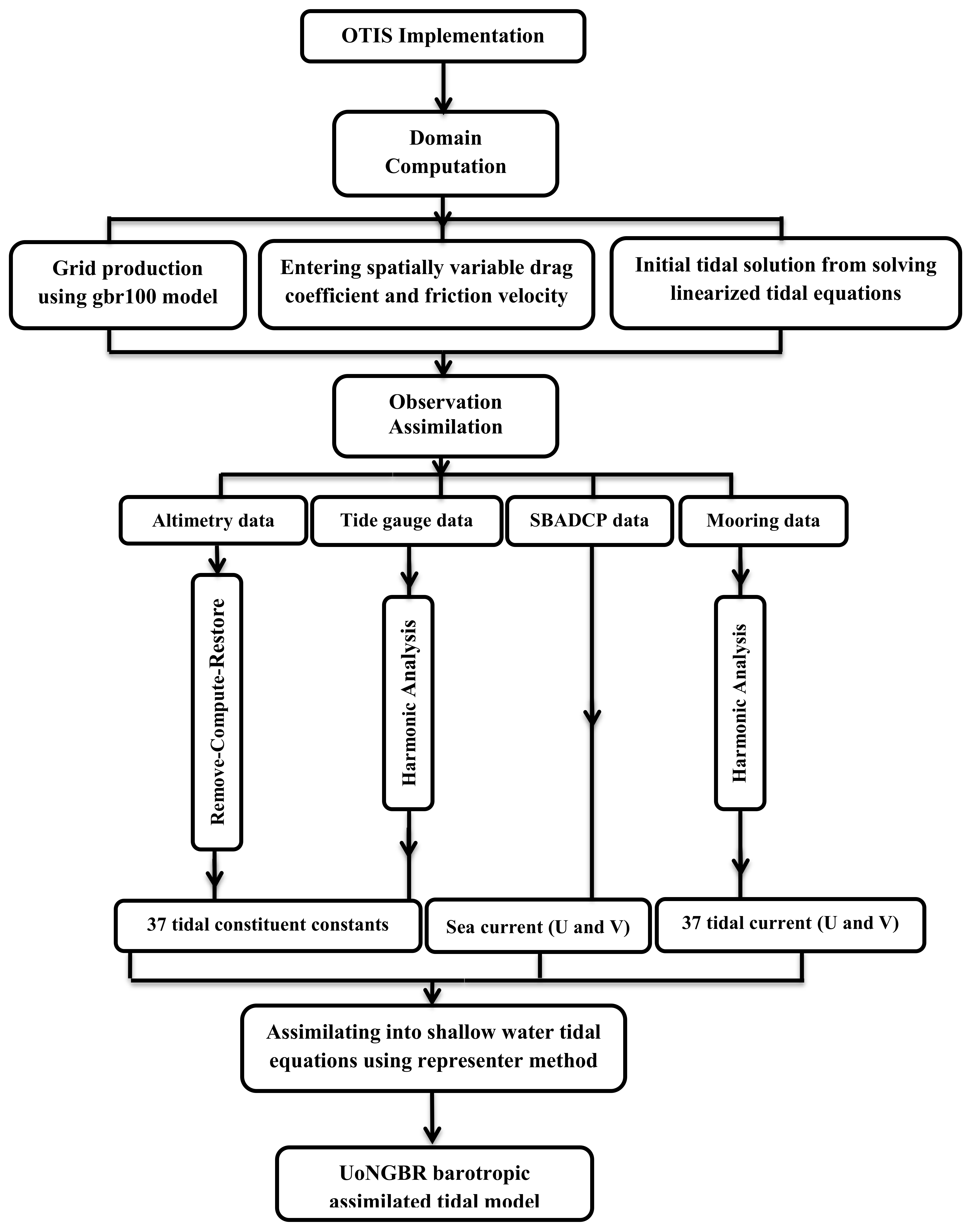
In this study, the Oregon State University Tidal Inversion Software (OTIS) by [28] is used to assimilate empirical observations into hydrodynamic equations in the GBR and Coral Sea. All available data and dynamics can be combined using the OTIS software tool to develop a new tidal model. This software uses a representer method [28] to assimilate available tidal data into shallow water equations. In this software a set of programs efficiently conduct representer calculation, generate efficient grids, prior model covariance, boundary conditions and implement tidal data inversion [29]. Compared to other assimilation algorithms, OTIS benefits from further simplifications, which facilitate tidal assimilation modelling over large scales but with limited computation expenses. In addition, further updates of this software provide users with capability of using sea surface current data from moorings and ship borne ADCPs [30].
The new tidal model for the GBR and Coral Sea developed in this study is named as the UoNGBR model. The resultant model has a spatial resolution of 2′ × 2′. It uses the most recent bathymetry model for the study area and addresses what role the reef plays in tidal behaviour of the region by accounting for variations of the drag coefficient over reef and non-reef areas. It includes 37 tidal constituents of major and shallow water types: M2, S2, K1, P1, N2, O1, Q1, S1, K2, 2N2, eps2, J1, L2, La2, R2, T2, M3, M4, M6, M8, MKS2, MK3, MN4, MS4, Mu2, Nu2, S4, N4, OO1, SO1, Mf, Mm, Sa, Ssa, Msf, Msqm and Mtm.
The remainder of the paper is structured as follows. The study area and datasets are described in Section 2. A description of implementing the model is presented in Section 3. In Section 4 sensitivity analysis of the contribution of bathymetry and drag coefficient data to the new model in the study area is discussed. The results, validations, conclusions and further discussions are presented in Section 5 and Section 6.

2. Study Area and Data

The study area is located in the GBR and Coral Sea, geographically extending from latitudes 10°S to 26°S and longitudes 142°E to 156°E and covering the continental shelf and slope of Queensland’s coastline, Australia. The GBR is located at the western margin of the Coral Sea with numerous reefs ranging in area from 0.01 to 100 km2, which has created a complex bottom topography and thus complex hydrodynamics [5,31].The average depth over the GBR is 35 m but plunging into more than 5000 m in the Coral Sea. Therefore, in this paper we define four different zones, namely coastline, coastal, shelf and (deep) ocean zones, according to bathymetry. The performance of the new tidal model UoNGBR will be evaluated over these zones (Figure 1).
The datasets used in the implementation and evaluation of UoNGBR are classified as model input and validation data. Both data types include satellite altimetry, coastal and marine observations that are further described in Section 2.1 and Section 2.2.

2.1. Input Data

The data from multi-satellite altimetry missions of Topex/Poseidon (T/P), Jason-1, Jason-2, Envisat and ERS-2 are used in the UoNGBR tidal modelling. Other input datasets include sea level and current measurements from coastal tide gauges, moorings and shipborne ADCP.

2.1.1. Multi-Satellite Altimetry Missions

During 1992–2002, the T/P altimeter provided unprecedented accurate observations of sea levels. Continuing on T/P’s observations and orbital arguments, the sea level was measured by Jason-1 from 2002 to 2009, and then followed by OSTM Jason-2 from 2009 to 2016. The current Jason-2 mission is still on the orbit and records sea level observations. Therefore, the sea level observation time series for this set of altimeter missions in this study is formed from 1992 to 2016, a total 25 years. The along-track distance between two successive footprints of a pass over the sea is about 7 km, while the distance between two passes is about 315 km at the equator. In addition, 3-year data from Jason-1’s interleaved orbit is also used in this study. These missions were specifically designed to study ocean dynamics, including circulations and tides [32]. Sea level observations from these missions are suitable to study ocean tides owing to their short repeat period of 9.9156 days and highly accurate orbital accuracy of few centimetres [33].
The ERS-2 and Envisat missions have a longer repeat period of 35 days, compared to that of the T/P series, and a smaller distance between two successive orbits at the equator. ERS-2 observed the sea level from 1995 to 2003, while Envisat extended the survey on the same orbit as ERS-2 from 2003 to 2010, producing altogether a valuable time-series of sea level observations. However, the sun-synchronous orbit of these missions fails to see sun-caused constituents such as S1, S2 and S4 [34]. The multi-mission altimetry data used in this study are available from the Radar Altimeter Database System (RADS, rads.tudelft.nl). The satellite data implemented in this study has been summarized in Table 1.

2.1.2. Coastal Tide Gauges

Sea-level observations recorded at 19 tide gauges between 1991 and 2015 (Table 2) were used in this study. The data have a high accuracy of 1 cm in all weather conditions [35] and a sample rate of one or half an hour. The tide gauge datasets are available from the Australian Bureau of Meteorology (BoM, http://www.bom.gov.au/oceanography/projects/abslmp/data/), Maritime Safety Queensland (http://www.msq.qld.gov.au/Tides/Open-data) and Permanent Service for Mean Sea Level (http://www.psmsl.org). The geographic distribution of tide gauges and altimetry tracks are depicted in Figure 2. The altimeter tracks are shown for T/P (in green), ERS-2/Envisat (in blue) and Sentinel-3A (in red). Tide gauge positions are shown in solid triangles.

2.1.3. Bathymetry

In order to address the importance of an accurate bathymetry model, two depth models of gbr100 [24] and General Bathymetric Chart of the Oceans (GEBCO) [36] are used in this study. The gbr100 bathymetry model uses the latest datasets obtained from ship-based multi-beam, single-beam and echo-sounder surveys, airborne LiDAR bathymetry surveys, and satellite remotely sensed data that is updated and delivered regularly. This model has a pixel size of 0.001-arc degree (or 3 arc seconds and is approximately 100 m) [24]. This model is available from the Deep Reef Explorer (https://www.deepreef.org/). The GEBCO model is the most publicly available depth model that provides bathymetry maps with different spatial resolutions at global and regional scales. This model benefits from new sounding data that has improved over shallow water regions. The GEBCO_2014 version of this bathymetry model with a spatial resolution of 30″ × 30″ is used in this investigation (http://www.gebco.net/data_and_products/gridded_bathymetry_data/). The accuracy of the bathymetry models has been determined as an approximate 0.5% of the depth value [37]. Thus, the deeper the grid node is located, the larger its depth error is expected to be. This source of error is due mainly to the sounding systematic and environmental associated errors [38], which escalate in deeper zones. The Mean Sea Level (MSL) is used as the height datum for depth values in both the gbr100 and GEBCO_2014 models [24,36].

2.1.4. Mooring Network

The National Mooring Network in Integrated Marine Observing System (IMOS, http://imos.org.au/) provides physical and biological measurements of Australian coastal waters for scientific research projects. More than nine permanent stations installed on the seabed bottom measure the meridional (V) and zonal (U) current velocities over the study area. These in-situ measurements are made on a 30 min temporal resolution. Table 3 shows the station name, geographic position and period of observation records for each current meter supplied by the IMOS.

2.1.5. Shipborne ADCP

The OTIS software has the capability of processing ship borne ADCP data [30]. The acoustic Doppler shift profilers can be mounted on voyage ships and record the zonal (U) and meridional (V) components of sea currents in different ocean depth layers and for numerous geographical positions along the ship sailing track. Figure 3 shows the locations of mooring stations and sail tracks of different voyages along which U and V components have been recorded. The ship-borne ADCP data are from the Commonwealth Scientific and Industrial Research Organisation’s (CSIRO) Marlin Metadata System (http://www.marlin.csiro.au).

2.1.6. Drag Coefficient Values

In assimilated tidal models, at either a global or regional scale, the drag coefficient is usually considered to be a constant value as the seabed is predominately sand over the majority of seas and oceans. However, studies in the eastern Irish Sea [39], northern Gulf of Mexico [40] and the North Sea [41] have revealed that the value of drag coefficients vary from 0.0025 to 0.0029 under different conditions. In the GBR region, it has been reported that different seabed types can pose spatially varying drag coefficient values [26]. This coefficient varies noticeably from 0.0025 to 0.0048 over the GBR and Coral Sea. When compared to the constant value (0.003) for sand beds, this is of a considerable difference. This fact leads to considering the drag coefficient as a variable parameter in our modelling procedure. The spatially varying drag coefficient value based on the GBR1 Hydrodynamics Model [27] is adopted in this study, which can be obtained from the GBR1 hydrodynamic model database (https://research.csiro.au/ereefs/).

2.2. Validation Data

In order to evaluate the efficiency of the UoNGBR model, recent satellite Sentinel-3A altimeter datasets (2016–2019) were used (Table 1). Data from Sentinel-3A can be considered as an independent dataset, as they have not been used by existing tidal models at the time of this study. This altimetry satellite is part of Sentinel missions designed to provide measurements for monitoring the global environment [42]. Sentinel-3A has a sun-synchronous orbit and repeats every 27 days. It has been designed to observe the sea surface with an approximate accuracy of 2–3 cm [43]. Over the coastline zone, the UoNGBR model was validated against three coastal tide-gauge stations that have not been used in the model development (Table 2). The distribution of Sentinel-3A tracks and validation tide gauges can be seen in Figure 2. In addition, the UoNGBR model was validated against seven existing tidal models. For this, the sea level anomalies that include tides (SLAt) were detided using seven existing tidal models: FES2012, FES2014, TPXO8, TPXO9, GOT 4.10, DTU10 and EOT11a. The detailed description of these models can be found in [15,44].

3. Modelling Procedure

The modelling procedure in this study comprises of two main phases. In the first phase an empirical model is developed based on analysing data from coastal tide gauges and multi-satellite altimetry missions. Then, this model is used at the second phase as the source of open boundary conditions for the initial solution in OTIS software.

3.1. Empirical Tidal Model

In order to develop the empirical tidal model, the Remove–Compute–Restore method is used. This is the most adopted and applied approach in geosciences, especially in geodesy. It has been widely used in modelling the regional geoid using satellite gravity data and developing semi-empirical tidal models in recent years [45,46,47,48,49]. In this approach a base model (FES2014) is used to remove tides from SLAt data to calculate the Sea Level Anomaly (SLA). The SLAs are then analysed to extract tidal corrections. Finally, the tidal corrections are added back to constituents interpolated from the base model.
In order to extract tidal constants for major and shallow water tidal constituents, both the harmonic analysis and response method are used. Tide-gauge data are analysed using the harmonic analysis, while for altimetry observations a combination of both harmonic and response approaches are used. The detailed description of the empirical model has been presented in [50]. The resultant 37 tidal constants of long-term, major and shallow water constituents are adopted as open boundary conditions in the forward solution of OTIS software.

3.2. Use of OTIS Software

The assimilation approach used in OTIS is a generalized inverse method (GIM), which is based on minimizing an explicitly defined penalty function [51]. It uses the GIM to assimilate data into the shallow water tidal equations. An explicitly defined penalty function, which includes both data and dynamics, is minimized using a least squares method [51]. The major difficulty in solving the GIM is the large size of the coefficient matrixes. For tackling this problem in OTIS an efficient representer method has been applied [52]. The large size of matrices can be reduced by eliminating velocities from shallow water equations, which decreases the number of unknowns [53]. However, instead of eliminating velocities, OTIS solves the linearized hydrodynamic equations using an iterative process that minimizes the penalty function [54]. For this purpose, an initial solution for the unknowns (i.e., tidal constituent constants) are calculated by solving linearized shallow water equations. Then, the initial solution is used through an iterative process to gain a solution that best fits both empirical observations and tidal hydrodynamic equations. The mathematical formulation of OTIS is briefly shown as follows [51,52,55]:
The empirical observations constitute equations as
d = L u
where d is the observation vector and L the measurement functions which relate the observed data to the unknown tidal state u. On the other hand, the tidal hydrodynamic equations are
S u = f 0
where u is the tidal state, including tidal zonal and meridional current components (U, V) and tidal height (ξ), S the matrix of hydrodynamic equations and f0 the astronomical forcing. Therefore, in the assimilation, the set of equations to be solved are of the form as
[ S L ] u = [ f 0 d ]
In order to estimate the true tidal state (u), Equation (3) must be solved. Although it is theoretically possible to find a solution of u0 which satisfies Equation (2), in general no tidal state (u) will satisfy Equation (3). This means that the operator, formed by a combination of data functional (L) and hydrodynamic (S) equations, is singular. The GIM, as used in OTIS, essentially constructs a generalized inverse of this operator [28]. Meanwhile, as there is no exact tidal state (u) to satisfy Equation (3), the inverse calculation is proposed as a fitting problem through an iterative process with both data and hydrodynamic constrains. However, the feasibility of this assimilation method has been of concern due to the size of matrices in computations. For tackling this problem in the representer approach, every element of data functional vector (Lk) is represented by element rk in the unknown parameters space (u), which is the reason that this method is known as representer approach. In the fitting iterative process, the final tidal state ( u ) is computed as
u = u 0 + k = 1 K b k r k
where b is the matrix of coefficients. Therefore, the inverse tidal problem in OTIS is based on the calculation of the representers (r) for the data functionals (L), and then solving Equation (4) in order to find the unknown vector ( u ). The location of these representers, according to the default of OTIS, is the altimetry crossover points where the empirical observations have a higher density.
In order to estimate 37 tidal constants using OTIS software in this study, the empirical model developed by [50] is used as the initial tidal model and consequently the source of open boundary conditions. The output of this stage will be an initial solution that is used in the assimilation procedure. Based on the features of OTIS, we design the modelling procedure of the UoNGBR model (Figure 4), which assimilates input data in GBR and Coral Sea into shallow water equations using OTIS software [56].
In the GBR, the mooring networks record the zonal (U) and meridional (V) velocities on a temporal resolution of 30 min (Table 3). These current meters mounted on the sea bottom are able to measure the sea current velocities at different depths (Figure 3). Therefore, we used the harmonic analysis to extract the amplitude and phase of U and V for tidal constituents that are to be assimilated using OTIS. In addition, the U and V from ADCP profiles shown in Figure 3 were also used in assimilation, as the OTIS software has the capability of processing shipborne ADCP data [30]. Furthermore, the tidal constants of 37 tidal constituents extracted from coastal tide-gauges (harmonic analysis) and satellite altimetry data (harmonic and response analysis) [50] are assimilated into hydrodynamic equations.
Before implementing OTIS software, in order to investigate the possible contribution of the new bathymetry model, gbr100, and spatially variable drag coefficient values to tidal modelling over the GBR, a sensitivity analysis was performed. The final output of OTIS implementation is the UoNGBR model with 37 tidal constituents.

4. Sensitivity Analysis

The hydrodynamics of shallow water regions, estuaries, straits and bays is affected by uncertainties in both bottom friction and bathymetric data [57,58,59,60,61]. Bathymetric data has been known as an important input to shallow water hydrodynamic modelling [62,63], while the influence of the drag coefficient value on tides in coastal regions has been reported by other studies [64,65].
Over coastal areas, the non-linearity of shallow water tidal equations is more important due to their contribution to complexity of the tidal spectrum in these regions [19,66]. This complex non-linearity results in shallow water tidal components being produced, which provide comparable amplitudes to some major constituents in coastal regions. The generation of these short wavelength waves is due to the interaction between major constituents with themselves or other components, which overall is caused by bottom topography and friction. In this section, a numerical assessment is implemented based on a sensitivity analysis to investigate the role of two main inputs of tidal hydrodynamic equations: Bathymetry and drag coefficients. For validation, Sentinel-3A and coastal tide gage data are used.
The sensitivity analysis was conducted using OTIS. In order to assess the improvement of bathymetry, both gbr100 and GEBCO models are considered. To evaluate the contribution of drag coefficient values, a constant value of 0.003, the default value in OTIS, and spatially variable drag coefficient values are considered. The test area subjected to this assessment is geographically bounded by longitudes 147°E to 153°E and latitudes 23°S to 19°S in the GBR.

4.1. Bathymetry Effects

This set of tests concerns the effect of different bathymetry models of gbr100 and GEBCO (cf. Section 2.1.3). First, the linearized shallow water equations are solved using the forward solution in OTIS software. This is done using depth from gbr100 and then GEBCO model, respectively, while keeping all other conditions unchanged in both implementations. Second, the estimated tidal constituents are used to predict the tidal height, which is consequently used to detide SLAts observed by Sentinel-3A and coastal tide gauges. Finally, the Root Mean Square (RMS) of the SLAs based on different bathymetry models (Table 4) are estimated and compared over coastline (CL), coastal (CZ), shelf (SZ) and deep ocean (OZ) zones (cf. Figure 1).
The results shown in Table 4 support that using a more accurate bathymetry model will generate a more efficient tidal model. The most significant contribution of gbr100 appears over coastline and coastal zones, where the difference between mean RMS errors of SLAs based on gbr100 and GEBCO is 15.9 cm and 13.7 cm, respectively. Over the shelf zone, the mean RMS error based on gbr100 is ~6 cm smaller than that based on GEBCO, while the difference of mean RMS errors can be neglected over the deep ocean zone. In order to further assess the difference between two models in estimating tidal constituents over four zones, eight semi-diurnal, diurnal and shallow water constituents (e.g., M2, S2, K1, P1, M4, M6, MK3 and S4) are considered. For a given constituent j, the RMS error of model difference is calculated as [67]
R M S j = ( 1 2 N i = 1 N ( H i g b r 100 H i G E B C O ) 2 ) 1 / 2
where N is the number of locations in a zone, and H the complex form of tidal amplitude and phase. Figure 5 shows the mean RMS errors of eight constitutes with the bathymetry gbr100 and GEBCO models. It can be seen that semi-diurnal constituents are mainly affected by the choice of bathymetry data when compared to shallow water constituents over this region. The M2 has a mean RMS of ~38 cm, ~25 cm and ~8.5 cm in coastline, coastal and shelf zones, respectively. The S2 has a mean RMS of ~15 cm, ~7.5 cm and ~3 cm in these three zones, respectively. Although the impact of bathymetry data on shallow water constituents is not considerable, M6 is more affected with the mean RMS error of ~0.4 cm and ~0.35 cm over the coastline and coastal zone, respectively. It was found that all types of constituents are insensitive to the selection of bathymetry data over the deep ocean zone.
It is acknowledged that the ocean bottom topography affects the coastal processes including tides. The tidal response of the oceans, wavelength of tidal waves proceeding to the coastline and interaction between major tidal constituents, that produces tidal shallow water components, are influenced by fluctuations of bathymetry [68,69,70]. Therefore, the high-resolution bathymetry model gbr100 significantly contributes to much more precise estimations of tidal constants than the GEBCO model.

4.2. Drag Coefficient Effects

The drag coefficient varies depending on the type of the sea bottom texture, which changes throughout the whole area of interest [26]. Most assimilative tidal models take this parameter as a constant value and assume that the sea bottom is mostly covered by sand. However, over the GBR and Coral Sea this parameter has been found to vary from 0.0025 to 0.0048 according to the GBR1 Hydrodynamics Model [27]. Therefore, in this section, the forward solution of OTIS software is used to assess the role of drag coefficient values in tidal modelling over the test area.
First, the linearized shallow water equations are solved with the OTIS default drag coefficient value (0.003). Second, a spatially varying drag coefficient value, which is one of the by-products of GBR1 hydrodynamic model, is used. Finally, the two models generated from the constant and varying drag coefficients are used to predict tidal heights and accordingly detide the sea level observations of coastal tide-gauges and SLAts from Sentinel-3A over the test area. Table 5 shows the numerical results of this statistical comparison. The mean RMS of calculated SLAs are estimated and discussed.
According to Table 5, over the coastline and coastal zones, the use of a spatially variable drag coefficient can better address the presence of the reefs over the study area. When comparing the results using varying drag coefficients to those using the constant coefficient, the mean RMS errors drop 2.1 cm, 1.8 cm, and 1.2 cm over CL, CZ and SZ zones, respectively. The results over the deep ocean zone show that models have the same quality no matter which types of drag coefficients are used. We also computed the mean RMS errors of the eight constituents with the constant and varying drag coefficients based on Equation 5 over four different zones (Figure 6).
From Figure 6, the drag coefficient mainly affects the semi-diurnal constituents, and less affects diurnal and shallow water constituents. The M2 has the maximum RMS errors of ~3.5 cm, ~3 cm and ~2.8 cm over coastline, coastal and shelf zones, respectively. The S2 has the second maximum RMS error around 1.0 cm over all zones, except for the deep ocean. Using the spatially variable drag coefficient or constant value does not significantly influence the diurnal constituents (RMS < 0.4 cm), and the shallow water constituents (RMS < 2 mm) in particular.
The drag coefficient is an important factor in determining the bottom friction in tidal hydrodynamics [71]. Tidal waves are interacting with seabed bottom on their way proceeding to coastal and shelf zones. Considering a realistic value for drag coefficients in a coastal region contributes to precise estimation of tidal constituents [72]. Therefore, accounting for variations of drag coefficients over coastline, coastal and shelf zones, induced by the type of the sea bottom, is another factor that contributes to the new assimilative tidal model over this area. Our sensitivity analysis results (Table 5 and Figure 6) suggest that using the spatially variable drag coefficient will better address the presence of reefs in an assimilative tidal model than using the constant value.

5. Results

From results shown in the sensitivity analysis in 
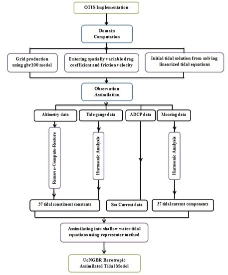
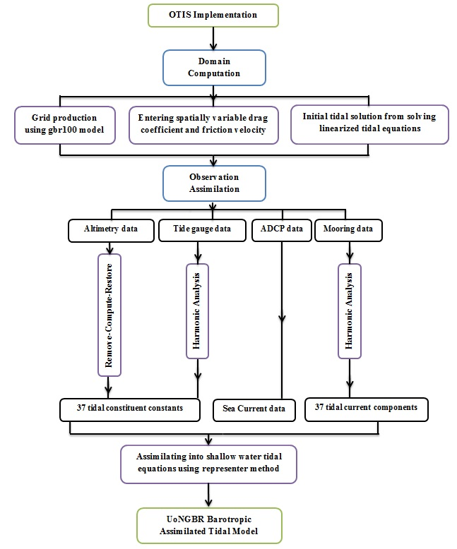
Section 4, it can be seen that over the GBR and Coral Sea, in particular over coastal and shelf zones, the high-resolution bathymetry and non-constant drag coefficient have to be considered. Followed the flowchart (Figure 4) and using the OTIS software, our assimilative tidal model UoNGBR was, thus, generated by the datasets from more than 25 years of satellite altimetry, coastal tide gauges, mooring and ship-born ADCP data, bathymetry model gbr100 and spatially varying drag coefficient values based on the GBR1 Hydrodynamics Model [
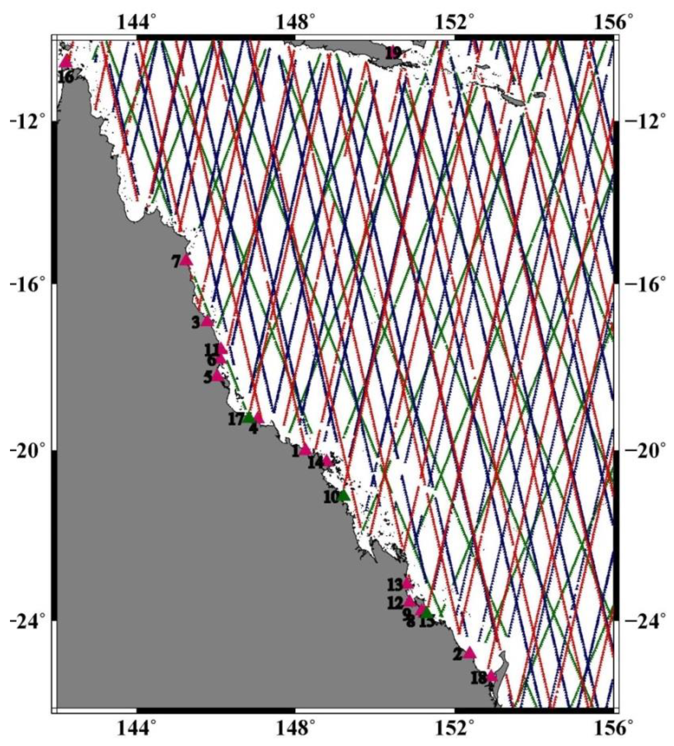
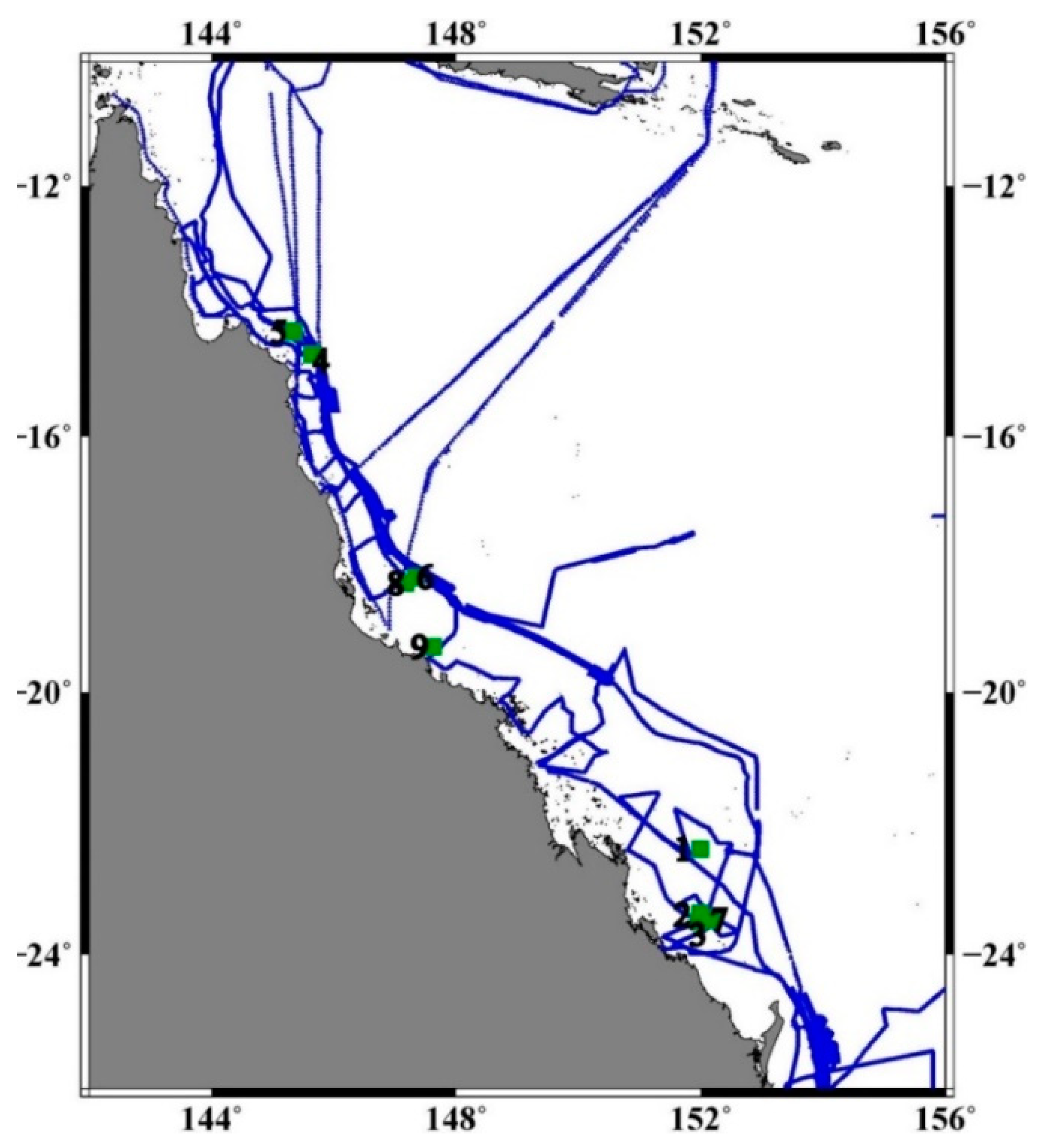
27]. In order to evaluate the efficiency of the UoNGBR model, coastal tide gauges and Sentinel-3A SLAts were used (cf. Figure 2). The results and performance of the UoNGBR model over the study area are discussed in this section.
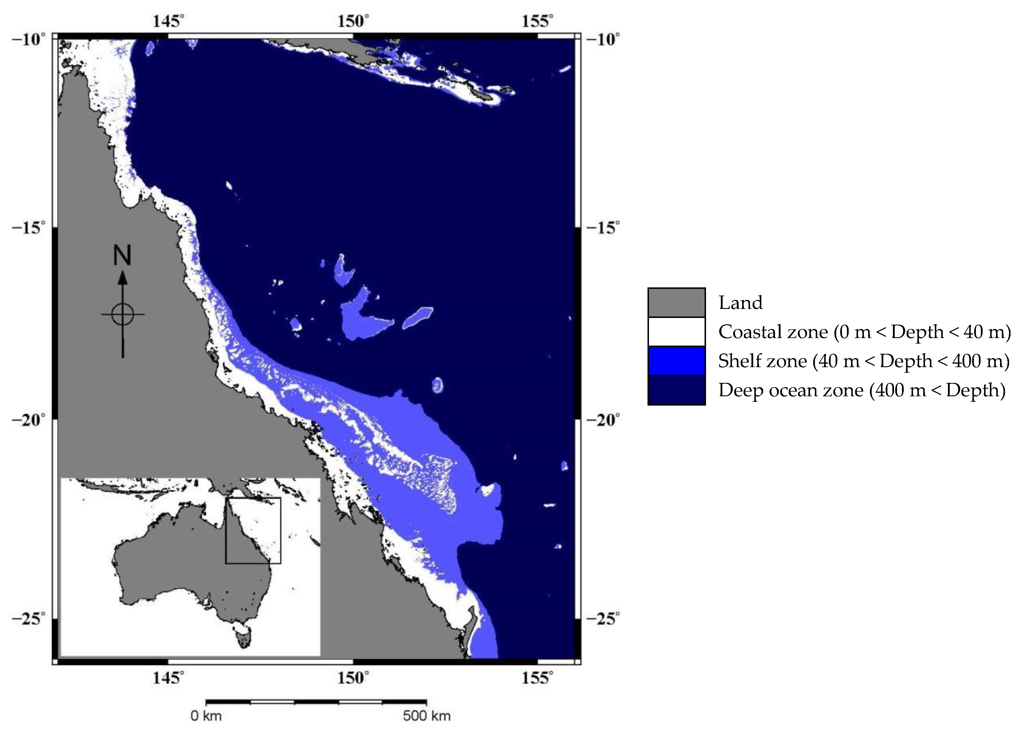
The performance of the UoNGBR model is assessed in four different zones (cf. Figure 1). For model validation, the UoNGBR-derived ocean tide corrections are used to detide the SLAts made by both tide gauges and Sentinel-3A. In addition, the SLAts are detided using other seven tidal models, including FES2012, FES2014, TPXO8, TPXO9, GOT 4.10, DTU10 and EOT11a. The RMS of the detided SLAs is then computed for each tidal model. The magnitude of RMS of the SLAs can be used to assess the efficiency of the tidal models, with the small RMS indicating the better performance of the model. The comparison among computed mean RMS errors are shown in Table 6 and Figure 7. In order to assess the overall performance of models, the Root Sum Square (RSS) of mean RMS values over all four zones were calculated from:
R S S = ( i = 1 4 R M S i 2 ) 1 / 2
In Table 6, both TPXO8 and TPXO9 have been implemented by the representer approach proposed in OTIS, which is the same approach as used for UoNGBR. It can be seen that UoNGBR performs more efficiently than TPXO9 and TPXO8 with the mean RMS differences (TPXO-UoNGBR) of 19.3 cm and 16.3 cm, respectively, over the coastline. In addition, mean RMS differences between TPXO models and UoNGBR over coastal and shelf zones are ~5 cm and ~3 cm, respectively. These noticeable mean RMS differences suggest that tidal estimations have been significantly improved in UoNGBR due to several reasons, such as using a more accurate bathymetry, spatial variable drag coefficients, editing the OTIS default for representer locations and including more tidal constituents. The major improvement lies in shallow water regions, where an accurate knowledge of bathymetry is crucial. According to Andersen (1999), the spatial advection of tidal energy from deep to shallow zones is proportional to the square of the water level. This fact reflects on the contribution of the accurate bathymetry used in UoNGBR (i.e., gbr100). Over the deep ocean zone, the three models of UoNGBR, TPXO9 and TPXO8 show similar performance.
The numerical results shown in Table 6 indicate that spatially varying drag coefficients make important contributions to efficiency of the assimilative tidal model UoNGBR. A seabed of reef type has large drag coefficient values compared to the sand seafloor [26]. In global tidal models, such as TPXO8 and TPXO9, the drag coefficient may be represented as a constant value, as the majority of sea and ocean beds is of sand type. However, for regional tidal models over GBR, due to the presence of reefs, neglecting the variations of drag coefficients can reduce the accuracy of the model. The UoNGBR is modelled using spatially varying drag coefficients with a more realistic representation of the seabed type, exposing the model to an accurate bottom friction and consequently more accurate tidal constituent amplitudes and phases.
While every altimetry along-track profile and tide gauge locations can be considered as representers, it is impractical to run OTIS due to the size of the matrices. Egbert et al. (1994) proposed that a subset of data locations can be used as representers to tackle matrix size issues. It has been found that the most efficient data locations to be used as representers are where higher density of observations exist [56]. Therefore, altimetry crossover points are ideal data locations to be considered as representer positions. However, through the modelling experiments it was found that the crossovers located close to the coastlines should be excluded. This is due to the errors associated with altimetry sea-level observations over shallow waters [73]. Thus, these altimeter crossovers were excluded from the list of representer locations, and were replaced by the closest tide gauge. This resulted in more accurate tidal height predictions from the UoNGBR model.
In the GBR area, empirical models (e.g., DTU10, GOT4.10 and EOT11a) fail to provide accurate tidal heights in comparison to UoNGBR (Table 6), as expected. Although both DTU10 and GOT 4.10 show more efficient results than EOT11a, they are far less accurate than UoNGBR, especially over coastline, coastal and shelf zones. FES2012 outperforms its successor, FES2014, with the mean RMS difference of ~3 cm over the coastline and coastal zones, while over the shelf and deep ocean zones they both are similar (RMS errors 8.8 cm vs. 8.9 cm). UoNGBR outperforms FES2012 (RMS errors 18.8 cm vs. 19.7 cm) and FES2014 (RMS errors 18.8 cm vs. 23.1 cm) over the coastline. In the coastal zone, this model is still more favourable with the mean RMS being ~1 cm and ~5 cm smaller than FES2012 and FES2014, respectively. The new UoNGBR model performs at the same accuracy level as FES2012 and FES2014 over the shelf and deep ocean zones.
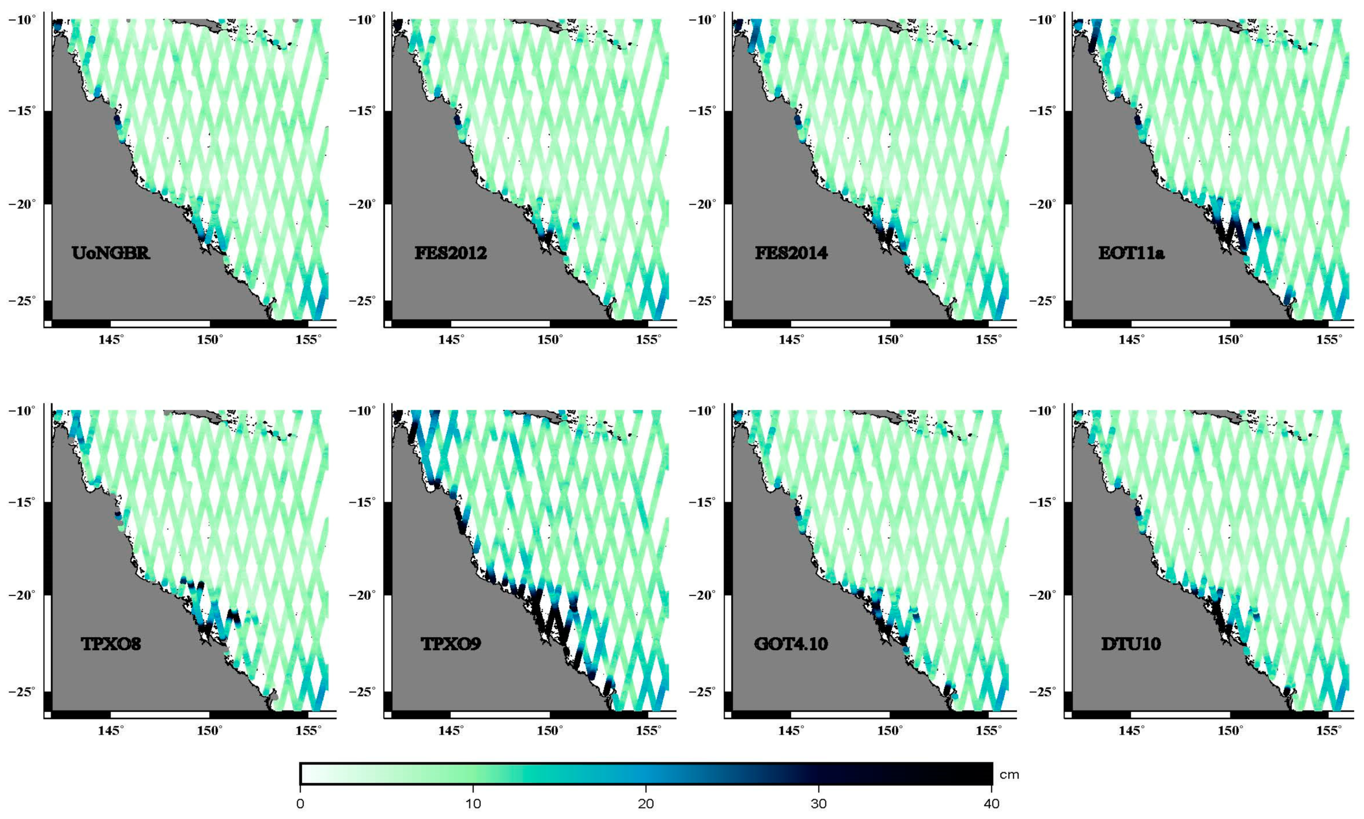
To assess the model capability of predicting tidal heights, Figure 7 shows the geographical distribution of calculated pointwise RMS values of SLAs over the study area. From Figure 7, it seems that all models act similarly in deep oceans, while in the shelf zone EOT11a is not as accurate as other models in terms of the tidal height prediction. The models of EOT11a, FES2014, TPXO9, GOT4.10 and DTU10 appear to have inefficiencies, with RMS errors > ~30 cm, in tidal high prediction over all or parts of this area. FES2012 shows an overall acceptable performance and is known as the best model for this region [44]. However, it is observed that FES2012 is slightly less accurate than UoNGBR at ~1 cm of mean RMS over coastline and coastal zone from Table 6. The area with large uncertainties along the coastline can be clearly seen in Figure 7.
The coastline and coastal zone are the main regions that model discrepancies are observed. Over these areas, UoNGBR shows a higher performance, followed by FES2012, GOT4.10 and DTU10. According to Figure 7, the area bounded by latitudes 20°S to 23°S and longitudes 146° to 151° is where large accuracy discrepancies are shown among models. Our previous study has found that there are sudden fluctuations in bottom topography due to existence of small islands [60], which is the main reason behind the model inefficiencies. Therefore, we defined this area as the challenging area [44]. Table 7 shows the performance of models in different zones of the challenging area.
Table 7 reveals the prime performance of UoNGBR over other models in the challenging area. The RSS differences between UoNGBR and FES2012, FES2014 and TPXO8 are ~4, ~21 and ~10 cm, respectively. The considerable difference in the challenging area between UoNGBR and other models mainly lays in coastal zones. Coastal zones in the challenging area include Broad Sound and the Southern GBR, where it is well known to have a complex tidal regime due to complicated bathymetry. Since this area is featured with high fluctuation of bathymetry, the superior efficiency of UoNGBR can be assigned to the use of the high-resolution bathymetry model gbr100. A closer look at the amplitude and phase of M
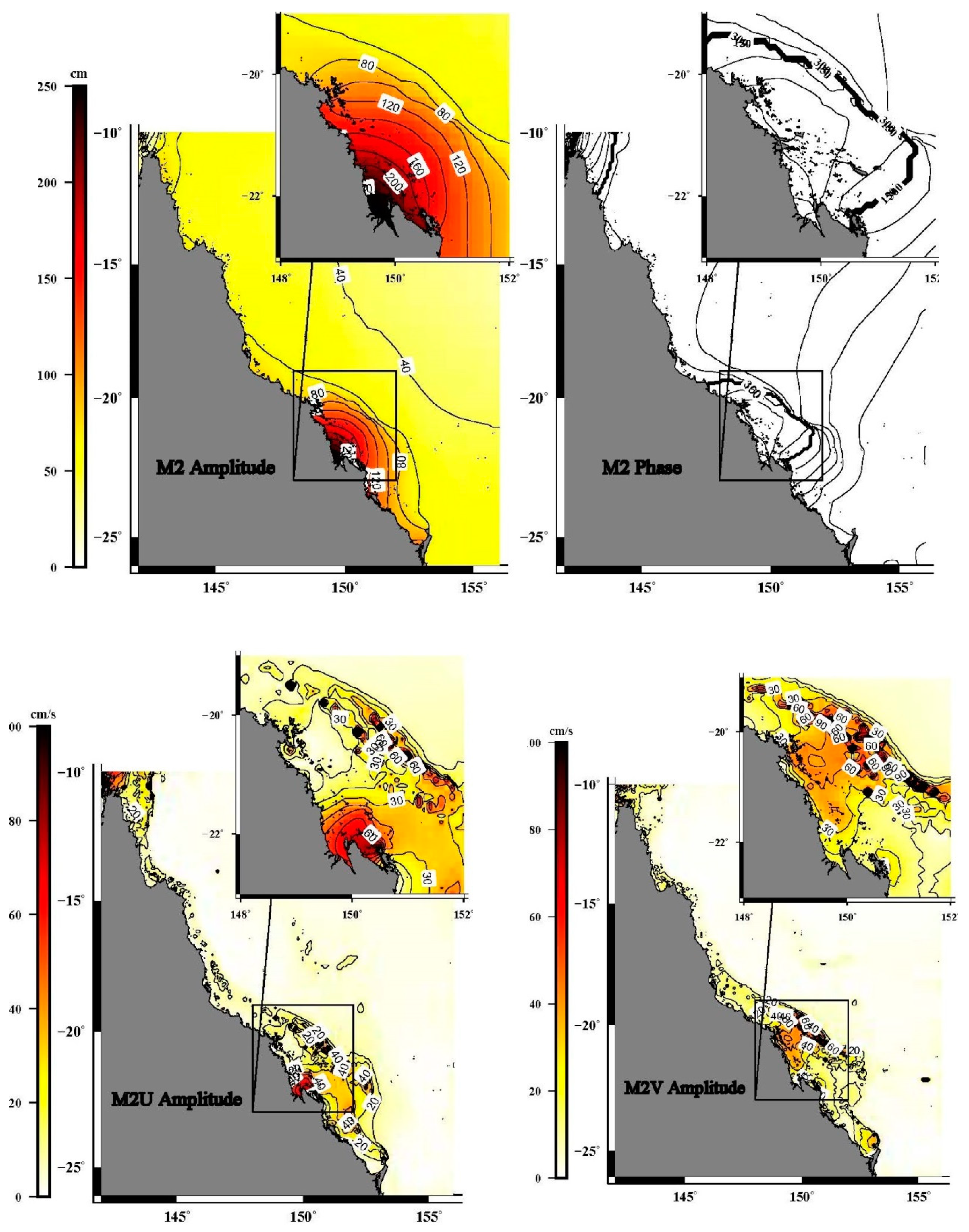
2, interpolated from the UoNGBR model, reveals why tidal models face difficulties in modelling the tidal wave over coastal zones especially in the challenging zone (Figure 8).
From Figure 8, it can be seen that over most of the GBR and Coral Sea the amplitude of M2 (top left) shows a monotonic behaviour. Over coastal zones, where most of coral reefs are located, this constituent’s amplitude is magnified, in particular in the challenging area, where amplitudes exceed more than 150 cm near the coastline. The intense variations can also be seen in the phase map (top right in Figure 8) over the continental slope, where the depth reduces from more than 2000 m to 100 m. This sudden variation in depth affects the phase and amplitude of long wavelength M2 waves, which are further magnified when proceeding to the coastline. This confirms the fact that accurate knowledge of the bottom geometry of this area is crucial, for which this study has addressed the issue by using the more accurate bathymetry model gbr100.
The U and V tidal current maps of M2 (bottom panels in Figure 8) show the fact how existence of small islands and coral reefs along the Queensland coastline shapes the pattern of tidal currents. While the tidal current speed is within a few cm/s over most of the study area, it exceeds 60 cm/s in the challenging zone. The tidal currents may contribute to (or threaten) growth and maintenance of the reef and its ecosystem health through exchanging nutrients and pollutants, as well as sediment and sand transport [9,74,75,76,77]. According to Figure 8, tidal currents in inner reefs are of high amplitudes, which play an important role in exchanging these materials on a daily basis.

6. Conclusions and Recommendations

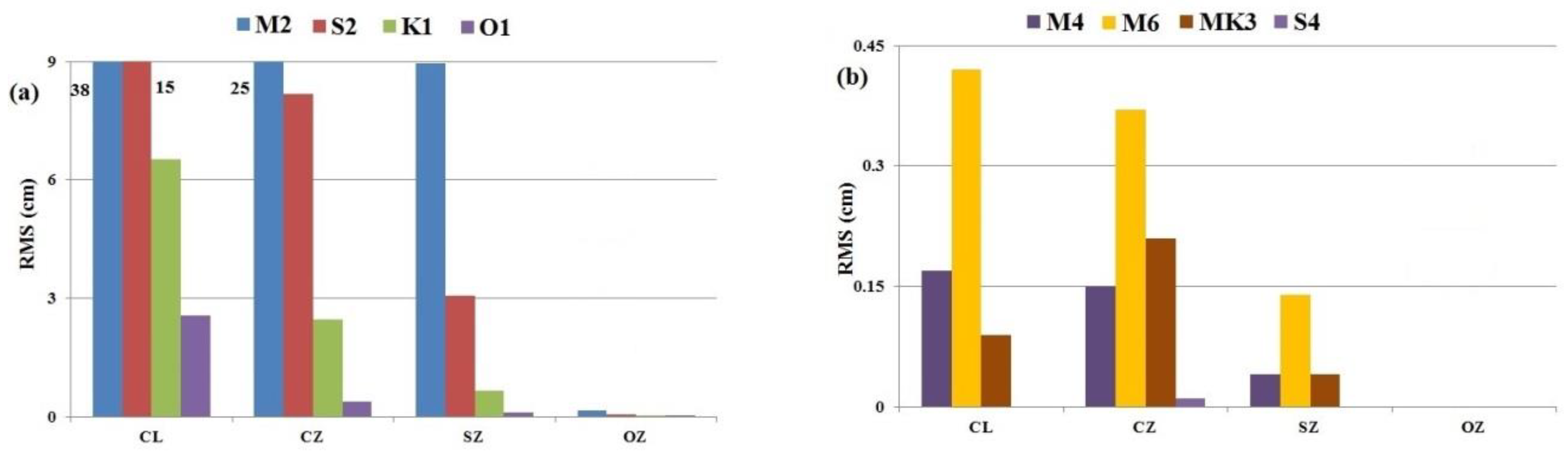
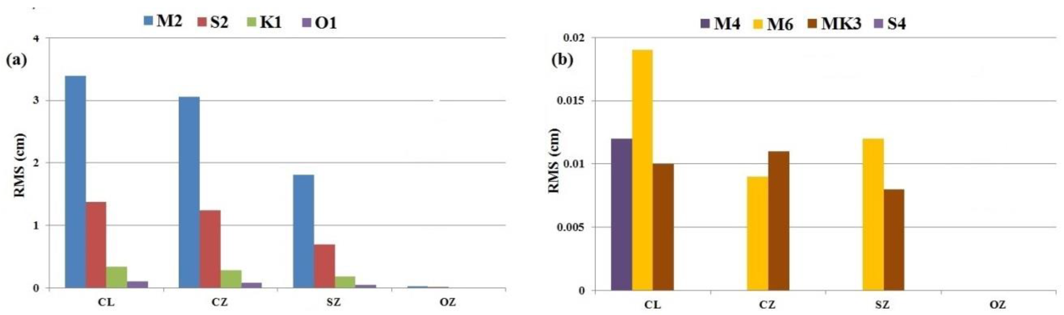
In this study, the UoNGBR barotropic assimilated tidal model was developed using OTIS software for the GBR and Coral Sea. All available satellite altimetry and coastal sea level observations and marine sea current data for the region are used to constraint the shallow water tidal equations. This model includes 37 major and shallow water tidal constituents that have been spread on a regular grid of 2’ × 2’. The influences of using the new bathymetry model, gbr100, and spatially variable drag coefficient were investigated in a sensitivity analysis and the results are shown in Figure 5 and Figure 6 and Table 3 and Table 4. The sensitivity analysis shows that using the high-resolution bathymetry model, gbr100, and spatially variable drag coefficients largely contribute to the estimation of major tidal constituents in this area. Since the new bathymetry has a high spatial resolution of 3.6″ × 3.6″, it is able to provide accurate information about sudden fluctuations in bathymetry due to the small islands and coral reefs. Figure 5 and Figure 6 reveal that new datasets improve the accuracy of major tidal constituents more than shallow water components. Our new tidal model benefited from detailed information about dynamics of the area, resulting in relatively superior performance to other models especially over areas with highly complex bottom topography. The UoNGBR data can be found in supplementary files associated with this paper.
There are challenges over the GBR region, which can be the main error sources for the UoNGBR model and thus subject to future studies. Some parts of the GBR region are too shallow at low tides and become deeper at high tides. This proposes the high rate of variations in bottom friction. Although the drag coefficient variations have been spatially considered in this study, their temporal variation features have not yet been investigated. In addition, the simplifications made in OTIS, such as using linearized shallow water equations, can be a source of error for the new model. Furthermore, a cross validation of how input datasets with different temporal and spatial scales affect the robustness of assimilated models should be considered in future studies.
The bathymetry in this study has been considered as constant in value. However, in reality due to the existence of numerous islands and coral reefs, bathymetry varies noticeably [6]. The constant bathymetry may not represent the reality of seafloor topography. In addition, while the 2′ × 2′ grid resolution was generated for the UoNGBR model, it is possible to use a multiple resolution grid for this area due to existence of the higher spatial resolution bathymetry [24]. In other words, a denser grid can be used over highly varying bathymetry areas, while the sparse grids can be taken over deeper ocean zones. Therefore, for future research, it is suggested that using higher order terms of bottom friction, time variant bathymetry and multi-resolution grids can further contribute to better understanding of tides in the GBR and Coral Sea.

Supplementary Materials

Supplementary File 1

Author Contributions

Conceptualization, F.S. and X.D.; METHODOLOGY and Validation, all authors; Software, F.S.; Formal Analysis and Investigation, F.S. and X.D.; Resources, all authors; Data Curation, F.S; Writing—Original Draft Preparation, F.S.; Writing—Review & Editing, all authors; Supervision, X.D. and O.B.A.; Funding Acquisition, X.D.

Funding

This research was funded by the Australian Research Council’s Discovery Project funding scheme (Project number DP150100615), and the International Tuition Fee Scholarship from the University of Newcastle, Australia.

Acknowledgments

The authors are thankful to AVISO and RADS for providing tidal models and altimetry data, to Australian Bureau of Meteorology and Maritime Safety Queensland for tide gauge data and CSIRO for providing mooring and ship-mounted ADCP data. We also would appreciate Robin Beaman for providing the latest version of gbr100 bathymetry model, Farhan Rizvi for access to high resolution spatially variable drag coefficient values and David Bretreger for proofreading the manuscript. The figures in this study were drawn with GMT software [78].

Conflicts of Interest

Authors declare that there is no conflict of interest. The sponsors had no role in any stage of this study.

References

  1. Dechnik, B.; Webster, J.M.; Webb, G.E.; Nothdurft, L.; Dutton, A.; Braga, J.-C.; Zhao, J.; Duce, S.; Sadler, J. The evolution of the Great Barrier Reef during the Last Interglacial Period. Glob. Planet. Chang. 2017, 149, 53–71. [Google Scholar] [CrossRef] [Green Version]
  2. Lambrechts, J.; Hanert, E.; Deleersnijder, E.; Bernard, P.-E.; Legat, V.; Remacle, J.F.; Wolanski, E. A multi-scale model of the hydrodynamics of the whole Great Barrier Reef. Estuar. Coast. Shelf Sci. 2008, 79, 143–151. [Google Scholar] [CrossRef]
  3. Choukroum, S. The Surface Circulation of the Coral Sea and Great Barrier Reef; James Cook University: Douglas, Australia, 2010. [Google Scholar]
  4. Mao, Y.; Luick, J.L. Circulation in the southern Great Barrier Reef studied through an integration of multiple remote sensing and in situ measurements. J. Geophys. Res. Ocean. 2014, 119, 1621–1643. [Google Scholar] [CrossRef]
  5. Legrand, S.; Deleersnijder, E.; Hanert, E.; Legat, V.; Wolanski, E. High-resolution, unstructured meshes for hydrodynamic models of the Great Barrier Reef, Australia. Estuar. Coast. Shelf Sci. 2006, 68, 36–46. [Google Scholar] [CrossRef]
  6. Lewis, A.; Hutchinson, S. Great Barrier Reef Depth and Elevation Model: GBRDEM; CRC Reef Research Centre: Townsville, Australia, 1994. [Google Scholar]
  7. Bode, L.; Mason, L.B.; Middleton, J.H. Reef parameterisation schemes with applications to tidal modelling. Prog. Oceanogr. 1997, 40, 285–324. [Google Scholar] [CrossRef]
  8. Wolanski, E. Tides on the Northern Great Barrier Reef Continental Shelf. J. Geophys. Res. Ocean. 1983, 88, 5953–5959. [Google Scholar] [CrossRef]
  9. Church, J.A.; Andrews, J.C.; Boland, F.M. Tidal currents in the central Great Barrier Reef. Cont. Shelf Res. 1985, 4, 515–531. [Google Scholar] [CrossRef]
  10. Middleton, J.H.; Buchwald, V.T.; Huthnance, J.M. The anomalous tides near Broad Sound. Cont. Shelf Res. 1984, 3, 359–381. [Google Scholar] [CrossRef]
  11. Andrews, J.C.; Bode, L. The tides of the central Great Barrier Reef. Cont. Shelf Res. 1988, 8, 1057–1085. [Google Scholar] [CrossRef]
  12. King, B.; Wolanski, E. Tidal current variability in the Central Great Barrier Reef. J. Mar. Syst. 1996, 9, 187–202. [Google Scholar] [CrossRef]
  13. Ray, R.D.; Egbert, G.D.; Erofeeva, S.Y. Tide Predictions in Shelf and Coastal Waters: Status and Prospects. In Coastal Altimetry; Vignudelli, S., Kostianoy, A.G., Cipollini, P., Benveniste, J., Eds.; Springer: Berlin/Heidelberg, Germany, 2011; pp. 191–216. [Google Scholar]
  14. Kivman, G.A. Assimilating data into open ocean tidal models. Surv. Geophys. 1997, 18, 621–643. [Google Scholar]
  15. Stammer, D.; Ray, R.D.; Andersen, O.B.; Arbic, B.K.; Bosch, W.; Carrere, L.; Cheng, Y.; Chinn, D.S.; Dushaw, B.D.; Egbert, G.D.; et al. Accuracy assessment of global barotropic ocean tide models. Rev. Geophys. 2014, 52, 243–282. [Google Scholar] [CrossRef] [Green Version]
  16. Smith, A.J.E.; Ambrosius, B.A.C.; Wakker, K.F.; Woodworth, P.L.; Vassie, J.M. Comparison between the harmonic and response methods of tidal analysis using TOPEX/POSEIDON altimetry. J. Geod. 1997, 71, 695–703. [Google Scholar] [CrossRef]
  17. Drecourt, J.P. Kalman Filtering in Hydrological Modelling; DAIHM: Horsholm, Denmark, 2003. [Google Scholar]
  18. Schumachaer, M. Assimilation of GRACE Data into a Global Hydrological Model Using an Ensemble Kalman Filter. Master’s Thesis, University of Bonn, Bonn, Germany, 14 September 2012. [Google Scholar]
  19. Egbert, G.D.; Erofeeva, S.Y.; Ray, R.D. Assimilation of altimetry data for nonlinear shallow-water tides: Quarter-diurnal tides of the Northwest European Shelf. Cont. Shelf Res. 2010, 30, 668–679. [Google Scholar] [CrossRef]
  20. Taguchi, E.; Stammer, D.; Zahel, W. Inferring deep ocean tidal energy dissipation from the global high-resolution data-assimilative HAMTIDE model. J. Geophys. Res. Ocean. 2014, 119, 4573–4592. [Google Scholar] [CrossRef]
  21. Carrere, L.; Lyard, F.; Cancet, M.; Guillot, A. FES2014, a new tidal model on the global ocean with enhanced accuracy in shallow seas and in the Arctic region. In Proceedings of the EGU General Assembly, Viena, Austria, 12–17 April 2015. [Google Scholar]
  22. Carrère, L.; Lyard, F.; Cancet, M.; Guillot, A.; Roblou, L. FES2012: A new global tidal model taking advantage of nearly 20 years of Altimetry. In Proceedings of the Meeting 20 Years of Radar Altimetry Symposiu, Venice, Italy, 24–29 September 2013. [Google Scholar]
  23. Egbert, G.D.; Erofeeva, S.Y. TPXO9, A New Global Tidal Model in TPXO Series. In Proceedings of the Ocean Sciences Meeting 2018, Portland, OR, USA, 11–16 February 2018. [Google Scholar]
  24. Beaman, R. A high-resolution depth model for the Great Barrier Reef and Coral Sea. In Proceedings of the RRRC GBR Operations Committee Meeting 10, Townsville, Australia, 12 August 2009. [Google Scholar]
  25. Cancet, M.; Lyard, F.; Birol, F.; Roblou, L.; Lamouroux, J.; Lux, M.; Jeansou, E.; Boulze, D.; Bronner, E. Latest improvements in tidal modelling: A regional approach. In Proceedings of the 20 Years of Progress in Radar Altimatry, Venice, Italy, 24–29 September 2013. [Google Scholar]
  26. McDonald, C.B.; Koseff, J.R.; Monismith, S.G. Effects of the depth to coral height ratio on drag coefficients for unidirectional flow over coral. Limnol. Oceanogr. 2006, 51, 1294–1301. [Google Scholar] [CrossRef]
  27. Herzfeld, M.; Andrewartha, J.; Baird, M.; Brinkman, R.; Furnas, M.; Gillibrand, P.; Hener, M.; Joehnk, K.D.; Jones, E.; McKinnon, D.; et al. eReefs Marine Modelling: Final Report; CSIRO: Hobart, Australia, 2016. [Google Scholar]
  28. Egbert, G.D.; Bennett, A.F.; Foreman, M.G. TOPEX/POSEIDON tides estimated using a global inverse model. J. Geophys. Res. Ocean. 1994, 99, 24821–24852. [Google Scholar] [CrossRef] [Green Version]
  29. Bennett, A.F. Inverse Methods in Physical Oceanography; Cambridge University Press: Cambridge, UK, 1992. [Google Scholar]
  30. Erofeeva, S.Y.; Padman, L.; Egbert, G. Assimilation of Ship-Mounted ADCP Data for Barotropic Tides: Application to the Ross Sea. J. Atmos. Ocean. Technol. 2005, 22, 721–734. [Google Scholar] [CrossRef] [Green Version]
  31. Brinkman, R.; Wolanski, E.; Deleersnijder, E.; McAllister, F.; Skirving, W. Oceanic inflow from the Coral Sea into the Great Barrier Reef. Estuar. Coast. Shelf Sci. 2002, 54, 655–668. [Google Scholar] [CrossRef]
  32. Gerold Siedler, J.G.J.C.; Siedler, G.; Church, J.A.; Gould, J.; Gould, W.J.; Church, P.J.A. Ocean Circulation and Climate: Observing and Modelling the Global Ocean; Elsevier Science: Amsterdam, The Netherlands, 2001. [Google Scholar]
  33. Martin, S.; Seelye, M. An Introduction to Ocean Remote Sensing; Cambridge University Press: Cambridge, UK, 2004. [Google Scholar]
  34. Bosch, W.; Savcenko, R.; Flechtner, F.; Dahle, C.; Mayer-Gurr, T.; Stammer, D.; Taguchi, E.; Ilk, K.-H. Residual ocean tide signals from satellite altimetry, GRACE gravity fields, and hydrodynamic modelling. Geophys. J. Int. 2009, 178, 1185–1192. [Google Scholar] [CrossRef] [Green Version]
  35. Permanent Committee on Tides and Mean Sea Level. Australian Tides Manual; PCTMSL: Wollongong, NSW, Australia, 2011. [Google Scholar]
  36. Jones, M.T. GEBCO User’s Guide; GEBCO: Merseyside, UK, 2014. [Google Scholar]
  37. Lalancete, M.F.; Debese, N. Analysis of bathymetry datasets quality: A margin case study. In Service Hydrographique et Océanographique de la Marine; GEBCO Symposium: Brest, France, 2009. [Google Scholar]
  38. Hare, R. Depth and position error budgets for multibeam echosounding. Int. Hydrogr. Rev. 1995, 72, 31. [Google Scholar]
  39. Green, M.O.; McCave, I.N. Seabed drag coefficient under tidal currents in the eastern Irish Sea. J. Geophys. Res. Ocean. 1995, 100, 16057–16069. [Google Scholar] [CrossRef]
  40. Safak, I. Variability of bed drag on cohesive beds under wave action. Water 2016, 8, 131. [Google Scholar] [CrossRef]
  41. Green, M.O.; Huntley, D.A.; Dyer, K.R.; Jago, C.F. Hydrodynamics and Sediment Dynamics of North Sea Sand Waves and Sand Banks and Discussion. Philos. Trans. Phys. Sci. Eng. 1993, 343, 461–474. [Google Scholar]
  42. Donlon, C.; Berruti, B.; Buongiorno, A.; Ferreira, M.-H.; Femenias, P.; Frerick, J.; Goryl, P.; Klein, U.; Laur, H.; Mavrocordatos, C.; et al. The Global Monitoring for Environment and Security (GMES) Sentinel-3 mission. Remote Sens. Environ. 2012, 120, 37–57. [Google Scholar] [CrossRef]
  43. Fletcher, K. Sentinel‑3: ESA’s Global Land and Ocean Mission for GMES Operational Services; European Space Agency: Toronto, ON, Canada, 2012. [Google Scholar]
  44. Seifi, F.; Deng, X.; Andersen, O.B. Assessment of the Accuracy of Recent Empirical and Assimilated Tidal Models for the Great Barrier Reef, Australia, Using Satellite and Coastal Data. Remote Sens. 2019, 11, 1211. [Google Scholar] [CrossRef]
  45. Yildiz, H.; Forsberg, R.; Ågren, J.; Tscherning, C.; Sjöberg, L. Comparison of remove-compute-restore and least squares modification of Stokes’ formula techniques to quasi-geoid determination over the Auvergne test area. J. Geod. Sci. 2012, 2, 53. [Google Scholar] [CrossRef]
  46. Sjöberg, L.E. A discussion on the approximations made in the practical implementation of the remove-compute-restore technique in regional geoid modelling. J. Geod. 2005, 78, 645–653. [Google Scholar] [CrossRef]
  47. Featherstone, W.; Holmes, S.A.; Kirby, J.; Kuhn, M. Comparison of Remove-Compute-Restore and University of New Brunswick Techniques to Geoid Determination over Australia, and Inclusion of Wiener-Type Filters in Reference Field Contribution. J. Surv. Eng. 2004, 130, 40–47. [Google Scholar] [CrossRef]
  48. Cheng, Y.; Andersen, O.B. Multimission empirical ocean tide modeling for shallow waters and polar seas. J. Geophys. Res. Ocean. 2011, 116. [Google Scholar] [CrossRef] [Green Version]
  49. Savcenko, R.; Bosch, W.; Dettmering, D.; Seitz, F. EOT11a—Global Empirical Ocean Tide Model from Multi-Mission Satellite Altimetry, with Links to Model Results PANGAEA; Deutsches Geodätisches Forschungsinstitut: Munich, Germany, 2012. [Google Scholar]
  50. Seifi, F.; Deng, X.; Andersen, O.B. A new empirical tidal model for the Great Barrier Reef, Australia. Eur. Geosci. Union 2018, 20, 18922. [Google Scholar]
  51. Egbert, G.D.; Bennett, A.F. Data assimilation methods for ocean tides. In Modern Approaches to Data Assimilation in Ocean Modeling, Volume 61; Malanotte-Rizzoli, P., Ed.; Elsevier: Amsterdam, The Netherlands, 1996; pp. 147–179. [Google Scholar]
  52. Egbert, G.D.; Erofeeva, S.Y. Efficient Inverse Modeling of Barotropic Ocean Tides. J. Atmos. Ocean. Technol. 2002, 19, 183–204. [Google Scholar] [CrossRef] [Green Version]
  53. Lyard, F.H. Data Assimilation in a Wave Equation: A Variational Representer Approach for the Grenoble Tidal Model. J. Comput. Phys. 1999, 149, 1–31. [Google Scholar] [CrossRef]
  54. Egbert, G.D. Tidal data inversion: Interpolation and inference. Prog. Oceanogr. 1997, 40, 53–80. [Google Scholar] [CrossRef]
  55. Egbert, G.D.; Bennett, A.F.; Foreman, M.G. TOPEX/POSEIDON tides estimated using a global inverse model. Oceanogr. Lit. Rev. 1995, 42, 513. [Google Scholar] [CrossRef]
  56. Egbert, G.D.; Erofeeva, S.Y. OSU Tidal Inversion Software Documentation. 2002. Available online: http://www-po.coas.oregonstate.edu/~poa/www-po/research/po/research/tide/inv_doc.html (accessed on 6 June 2018).
  57. French, J.R. Hydrodynamic Modelling of Estuarine Flood Defence Realignment as an Adaptive Management Response to Sea-Level Rise. J. Coast. Res. 2008, 24, 1–12. [Google Scholar] [CrossRef]
  58. Piedra-Cueva, I.; Fossati, M. Residual currents and corridor of flow in the Rio de la Plata. Appl. Math. Model. 2007, 31, 564–577. [Google Scholar] [CrossRef]
  59. Sousa, M.; Dias, J. Hydrodynamic Model Calibration for a Mesotidal Lagoon: The Case of Ria de Aveiro (Portugal). J. Coast. Res. 2007, 1075–1080. [Google Scholar]
  60. Zheng, L.; Chen, C.; Liu, H. A modeling study of the Satilla River estuary, Georgia. I: Flooding-drying process and water exchange over the salt marsh-estuary-shelf complex. Estuaries 2003, 26, 651–669. [Google Scholar] [CrossRef]
  61. Li, C.; Valle-Levinson, A.; Atkinson, L.P.; Wong, K.C.; Lwiza, K.M.M. Estimation of drag coefficient in James River Estuary using tidal velocity data from a vessel-towed ADCP. J. Geophys. Res. Ocean. 2004, 109. [Google Scholar] [CrossRef]
  62. Cea, L.; French, J.R. Bathymetric error estimation for the calibration and validation of estuarine hydrodynamic models. Estuar. Coast. Shelf Sci. 2012, 100, 124–132. [Google Scholar] [CrossRef]
  63. Bricheno, L.M.; Wolf, J.; Islam, S. Tidal intrusion within a mega delta: An unstructured grid modelling approach. Estuar. Coast. Shelf Sci. 2016, 182, 12–26. [Google Scholar] [CrossRef] [Green Version]
  64. Adcock, T.A.A.; Draper, S.; Houlsby, G.T.; Borthwick, A.G.L.; Serhadlıoğlu, S. The available power from tidal stream turbines in the Pentland Firth. Proc. R. Soc. A Math. Phys. Eng. Sci. 2013, 469, 20130072. [Google Scholar] [CrossRef] [Green Version]
  65. Gillibrand, P.A.; Walters, R.A.; McIlvenny, J. Numerical Simulations of the Effects of a Tidal Turbine Array on Near-Bed Velocity and Local Bed Shear Stress. Energies 2016, 9, 852. [Google Scholar] [CrossRef]
  66. Andersen, O.B. Shallow water tidal determination from altimetry—The M4 constituent. Boll. di Geofis. Teor. ed Appl. 1999, 40, 427–437. [Google Scholar]
  67. King, M.A.; Padman, L. Accuracy assessment of ocean tide models around Antarctica. Geophys. Res. Lett. 2005, 32. [Google Scholar] [CrossRef]
  68. Andersen, O.B. Shallow water tides in the northwest European shelf region from TOPEX/POSEIDON altimetry. J. Geophys. Res. Ocean. 1999, 104, 7729–7741. [Google Scholar] [CrossRef]
  69. Cheng, R.T. Tides, Tidal and Residual Currents in San Francisco Bay California—Results of Measurements, 1979–1980; U.S. Geological Survey, Water Resources Division: Sunrise Valley Drive Reston, VA, USA, 1984.
  70. Prandle, D. Estuaries: Dynamics, Mixing, Sedimentation and Morphology; Cambridge University Press: Cambridge, UK, 2009. [Google Scholar]
  71. Lee, J.C.; Kim, C.S.; Jung, K.T. Comparison of Bottom Friction Formulations for Single-Constituent Tidal Simulations in Kyunggi Bay. Estuar. Coast. Shelf Sci. 2001, 53, 701–715. [Google Scholar] [CrossRef]
  72. Wang, D.; Liy, Q.; Lv, X. A Study on Bottom Friction Coefficient in the Bohai, Yellow, and East China Sea. Math. Probl. Eng. 2014, 2014, 7. [Google Scholar] [CrossRef]
  73. Deng, X.; Featherstone, W.E. A coastal retracking system for satellite radar altimeter waveforms: Application to ERS-2 around Australia. J. Geophys. Res. Ocean. 2006, 111. [Google Scholar] [CrossRef] [Green Version]
  74. Burrage, D.M.; Steinberg, C.R.; Skirving, W.J.; Kleypast, J.A. Mesoscale circulation features of the great barrier reef region inferred from NOAA satellite imagery. Remote Sens. Environ. 1996, 56, 21–41. [Google Scholar] [CrossRef]
  75. Luick, J.L.; Mason, L.; Hardy, T.; Furnas, M.J. Circulation in the Great Barrier Reef Lagoon using numerical tracers and in situ data. Cont. Shelf Res. 2007, 27, 757–778. [Google Scholar] [CrossRef]
  76. Andutta, F.P.; Ridd, P.V.; Wolanski, E. The age and the flushing time of the Great Barrier Reef waters. Cont. Shelf Res. 2013, 53, 11–19. [Google Scholar] [CrossRef] [Green Version]
  77. Hamylton, S.M.; Carvalho, R.C.; Duce, S.; Roelfsema, C.M.; Vila-Concejo, A. Linking pattern to process in reef sediment dynamics at Lady Musgrave Island, southern Great Barrier Reef. Sedimentology 2016, 63, 1634–1650. [Google Scholar] [CrossRef] [Green Version]
  78. Wessel, P.; Smith, W.H.F. New version of the generic mapping tools. Eos Trans. Am. Geophys. Union 1995, 76, 329. [Google Scholar] [CrossRef]
Figure 1. The bathymetry of the GBR based on the gbr100 model. It covers the deep ocean (dark blue), shelf (steel blue) and coastal (white) zones.
Remotesensing 11 02234 g001
Figure 2. Spatial distribution of altimeter ground tracks and tide gauge locations. Tracks are shown for T/P (in green), ERS-2/Envisat (in blue) and Sentinel-3A (in red), while tide gauges are shown in solid triangles. Of them, Sentinel-3A (in red) and three tide gauges (in green triangles) are used as validation datasets.
Remotesensing 11 02234 g002
Figure 3. The mooring network (green squares) and ship borne acoustic doppler current profiler (ADCP) tracks (in blue) in the study area.
Remotesensing 11 02234 g003
Figure 4. The flowchart demonstrating the implementation of the UoNGBR model with OTIS software. The U and V are tidal zonal and meridional current components, respectively.
Remotesensing 11 02234 g004
Figure 5. The mean RMS errors of the difference between two bathymetry models in estimating four major (a) and four shallow water (b) constituents. The RMS value in (a) is >9 cm. The values over Ocean Zone (OZ) are equal or close to zero.
Remotesensing 11 02234 g005
Figure 6. The mean RMS values of the difference between two models, developed based on constant and varying drag coefficient value, in estimated four major (a) and four shallow water (b) constituents. The values over Ocean Zone (OZ) are equal or close to zero.
Remotesensing 11 02234 g006
Figure 7. The pointwise RMS values shown along Sentinel-3A tracks.
Remotesensing 11 02234 g007
Figure 8. The M2 amplitude, Greenwich phase and its current components U and V. The inset shows these quantities in more detail in the challenging area.
Remotesensing 11 02234 g008
Table 1. The satellite data used in this study.
MissionYearsRepeat Period (Days)Cross Track Distance in GBR (km)Type *
T/P + Jason-1 + Jason-21992–20169.9156300I
Jason-1 Phase B2009–20129.9156300I
ERS-2 + Envisat1995–20103576I
Sentinel-3A2016–20192799V
* “I” stands for input and “V” for validation data.
Table 2. The geographic position and period of observation records for coastal tide gauges.
Station No.Tide Gauge DameLatitude (Degrees)Longitude (Degrees)Time DurationType *
Start DateEnd Date
1Bowen Storm−20.01148.2501/01/199631/12/2015I
2Bundaberg−24.76152.3801/01/199631/12/2015I
3Cairns Storm−16.93145.7801/01/199631/12/2010I
4Cape Ferguson−19.26147.0501/01/199631/12/2015I
5Cardwell−18.25146.0301/09/199131/12/2015I
6Clump Point−17.83146.101/01/199731/12/2015I
7Cook Town−15.45145.2501/01/199631/12/2015I
8Fishermans Landing−23.78151.1601/01/200231/12/2015I
9Gladstone−23.83151.2501/01/199631/12/2015I
10Mackay−21.1149.2101/01/199631/12/2006V
11Mourilyan−17.6146.1101/01/199631/12/2015I
12Port Alma−23.58150.8601/01/199631/12/2015I
13Rosslyn Bay−23.16150.801/01/200131/12/2015I
14Shute Harbour−20.28148.7801/01/199631/12/2015I
15South Trees−23.85151.301/01/199631/12/2015V
16Thursday Island−10.56142.2101/01/199631/12/2015I
17Townsville−19.25146.8301/01/199631/12/2011V
18Urangan−25.3152.9101/01/199631/12/2015I
19Alotau−10.31150.4501/01/199631/12/2015I
* “I” stands for input and “V” for validation data.
Table 3. The geographic position and period of observation records for mooring stations.
Mooring No.Mooring Station CodeLatitude (Degrees)Longitude (Degrees)Time Duration
Start DateEnd Date
1GBRCCH−22.4083151.994527/04/200902/10/2017
2GBRHIN−23.3836151.987016/10/200907/10/2012
3GBRHIS−23.5123151.955312/09/200705/10/2017
4GBRLSH−14.1718145.641203/06/200919/05/2014
5GBRLSL−14.3393145.343423/04/201120/05/2012
6GBRMYR−18.2184147.344806/06/200915/11/2017
7GBROTE−23.4830152.172817//08/201131/03/2017
8GBRPPS−18.3103147.163425/10/201217/11/2017
9NRSYON−19.3051147.622023/06/200826/09/2017
Table 4. Mean root mean square (RMS) of sea level anomalies (SLAs) based on bathymetry models gbr100 and GEBCO in the test area (cm).
ZoneMean RMS Based on gbr100Mean RMS Based on GEBCO
CL37.853.7
CZ17.831.5
SZ11.517.0
OZ6.66.7
Table 5. The role of drag coefficient values—mean RMS errors of SLA differences (cm).
ZoneMean RMS Based on Spatially Varying Drag CoefficientsMean RMS Based on the Constant Drag Coefficient
CL37.840.1
CZ17.819.6
SZ11.512.7
OZ6.66.6
Table 6. The mean RMS (cm) of the SLAs and Root Sum Square (RSS) (cm) in the study area with the bold value indicating the minimum mean RMS (or RSS).
ModelCoastlineCoastal ZoneShelf ZoneDeep Ocean ZoneRSS
UoNGBR18.811.68.88.125.1
FES201219.712.38.88.026.1
FES201423.116.48.98.130.8
TPXO835.116.010.48.240.8
TPXO938.117.411.28.344.2
GOT 4.1024.614.710.38.131.5
DTU1033.215.37.710.638.9
EOT11a56.329.517.910.466.7
Table 7. The mean RMS of the SLAs in the challenging area over different zones (cm) with bold value indicating the minimum mean RMS.
ModelCoastlineCoastal ZoneShelf ZoneDeep Ocean ZoneRSS
UoNGBR26.811.59.18.731.9
FES201231.113.19.18.636.0
FES201444.624.49.68.652.4
TPXO832.822.810.78.742.2
TPXO935.922.913.78.845.2
GOT 4.1029.218.611.38.537.4
DTU1028.621.111.88.733.7
EOT11a58.139.122.310.574.2

