Abstract
Near-real-time (NRT) satellite-based rainfall estimates (SREs) are a viable option for flood/drought monitoring. However, SREs have often been associated with complex and nonlinear errors. One way to enhance the quality of SREs is to use soil moisture information. Few studies have indicated that soil moisture information can be used to improve the quality of SREs. Nowadays, satellite-based soil moisture products are becoming available at desired spatial and temporal resolutions on an NRT basis. Hence, this study proposes an integrated approach to improve NRT SRE accuracy by combining it with NRT soil moisture through a nonlinear support vector machine-based regression (SVR) model. To test this novel approach, Ashti catchment, a sub-basin of Godavari river basin, India, is chosen. Tropical Rainfall Measuring Mission (TRMM) Multisatellite Precipitation Analysis (TMPA)-based NRT SRE 3B42RT and Advanced Scatterometer-derived NRT soil moisture are considered in the present study. The performance of the 3B42RT and the corrected product are assessed using different statistical measures such as correlation coefficient (CC), bias, and root mean square error (RMSE), for the monsoon seasons of 2012–2015. A detailed spatial analysis of these measures and their variability across different rainfall intensity classes are also presented. Overall, the results revealed significant improvement in the corrected product compared to 3B42RT (except CC) across the catchment. Particularly, for light and moderate rainfall classes, the corrected product showed the highest improvement (except CC). On the other hand, the corrected product showed limited performance for the heavy rainfall class. These results demonstrate that the proposed approach has potential to enhance the quality of NRT SRE through the use of NRT satellite-based soil moisture estimates.
1. Introduction
Accurate measurement of rainfall in near-real-time (NRT) is a primary requirement for forecasting and monitoring of floods [1,2]. Ground-based rain gauges provide reliable point rainfall values [3]. However, these ground-based rainfall values are often not available in NRT, especially in developing nations of Asia and Africa. Even the available ones are scarcely distributed, which makes the accuracy of areal rainfall questionable [4]. With the emergence of space-based sensors, plenty of satellite-based rainfall datasets, such as Climate Prediction Center MORPHing technique (CMORPH)[5], Global Satellite Mapping of Precipitation (GSMaP) [6], Indian National Satellite System Multispectral Rainfall Algorithm (IMSRA) [7,8], Tropical Rainfall Measuring Mission Multisatellite Precipitation Analysis (TMPA) [9], and Integrated Multi-satellitE Retrievals for Global Precipitation Measurement (IMERG) [10], are now available in NRT in the public domain with good spatial and temporal resolutions. Hence, satellite-based NRT rainfall estimates can be used as an alternative for forecasting and monitoring of disasters such as floods and droughts.
Several evaluation studies of satellite-based rainfall estimates (SREs) have been conducted across the world [11,12,13,14,15,16] to ascertain their accuracy. Most of the studies have concluded that SREs are associated with errors, and the magnitude of errors varies with season, region, intensity, and topography [17,18,19,20,21,22]. Even though NRT SREs are associated with more errors when compared to the postprocessed SREs [23,24,25,26,27], they are preferred over the postprocessed product for disaster monitoring, such as flood and drought. The postprocessed estimates are unavailable in NRT, due to the lack of ground-based rainfall observations, which is an essential requirement to improve the NRT SREs during postprocessing stage [19]. At the same time, the direct use of NRT SREs for disaster monitoring is problematic, as they are associated with large errors especially at local and catchment scales [28,29,30]. Hence, it is essential to employ error reduction methods to improve the NRT SREs before their application [31].
Various researchers have attempted to reduce the error or bias in SREs using different methods such as mean correction factor method [32], quantile mapping [33], and Bayesian approach [34]. However, these methods are associated with various limitations. For example, the mean correction factor method corrects only the mean value of the rainfall observations but does not correct the variance. Details of the limitations associated with these methods are given in [35,36]. Moreover, the error associated with SRE is very complex in nature due to its dependency on several factors, such as topography, location, climate, season, and rainfall intensities [37,38,39,40]. To overcome these issues, several authors [41,42] have used SREs along with topography and location variables to reduce error through a linear parametric model. However, the major limitations in these approaches are related to the assumption of the statistical distribution of rainfall and the presence of nonlinearity in the error [43]. These limitations can be overcome by using machine learning approaches [43,44]. For example, Yang and Luo [43] adopted an artificial neural network (ANN) approach to correct SREs by using topographic and location variables. Recently, Bhuiyan et al. [44] developed a nonparametric statistical model combining various SREs, reprocessed products, satellite-based soil moisture, and terrain variables to obtain a reliable reference rainfall product. Hence, it can be concluded that machine learning approaches have enough potential to combine several variables (static and dynamic) to improve SREs.
In a recent review, Maggioni and Massari [45] suggested merging soil moisture observations with satellite rainfall retrievals to improve rainfall estimates as the signature of soil moisture can persist from a few hours to several days after a rain event. Crow et al. [46] used soil moisture to correct the satellite-based rainfall estimates through a simple data assimilation approach and obtained an improved product. To follow up, Crow et al. [47] developed Soil Moisture Analysis Rainfall Tool (SMART) based on a relatively complex data assimilation and modelling approach using soil moisture and obtained even better results than Crow et al. [46]. Bhuiyan et al. [44] also found that the soil moisture is an important predictor to obtain a reliable reference rainfall product. However, ground-based soil moisture observation is rare and often limited to a few farms. Thus, remotely sensed soil moisture can be used to fill this gap. In the recent past, several studies have used satellite-based soil moisture [48,49,50,51,52] to obtain improvements in stream-flow prediction and rainfall estimations. These studies highlight the excellent capability of satellite-based soil moisture for hydrometeorological applications.
Considering the above facts, in this study, a machine learning approach called the support vector machine-based regression (SVR) model is chosen, in which NRT SRE is improved using satellite-based NRT soil moisture. As per the authors’ knowledge, this is the first study where NRT SRE is integrated with NRT soil moisture in a machine learning framework to improve NRT SRE. This article is organized into four sections: Following this introduction section, material and methods used are given in Section 2. The results and discussions of various analyses carried out are provided in Section 3. Finally, summary and conclusions of the study are described in Section 4.
2. Material and Methods
2.1. Study Area
The Ashti catchment is the test site for this study, which is a sub-basin of the Godavari River basin, India. The extent of this catchment lies between 78°0′ and 81°0′ East longitudes and 19°30′ and 22°50′ North latitudes, covering an area of approximately 50,000 km2. The elevation of the catchment varies from 144 to 1036 m above sea level [53]. Agricultural lands and forests are the major land use over the catchment [54]. Figure 1 represents the location of the catchment in India along with the observed monsoonal average rainfall during the study period. There are 86 rainfall grids of 0.25° × 0.25° spatial resolution enclosing the catchment. The entire study area is in the rainfed region and falls under the tropical climate zone. Most of the annual rainfall over Ashti catchment occurs during the southwest monsoon period between mid-June and mid-October [55]. Therefore, only the monsoon season is considered in the present study. The observed monsoonal average rainfall during study period varies from 1100 to 2100 mm in the rainfall grids over Ashti catchment (Figure 1b). Significant spatial variability in rainfall, complexity in terrain, and high vulnerability to floods make the Ashti catchment a suitable test site for the present study.
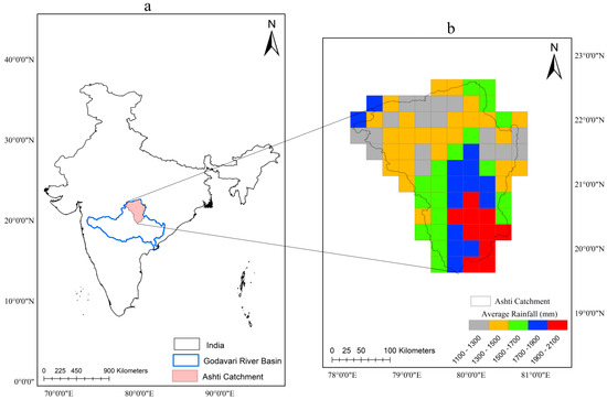
Figure 1.
(a) Location of the Ashti catchment and (b) Ashti catchment along with the observed monsoon average rainfall of each rainfall grids at a spatial resolution of 0.25° × 0.25° during the study period (Monsoon seasons 2012–2015).
2.2. Datasets
The datasets include rainfall and soil moisture estimates. The monsoon seasons of 2012–2015 are considered as the time span for this study. The time period is constrained by the availability of: (i) ground-based rainfall observations (up to 2015); and (ii) a consistent data record for Advanced Scatterometer (ASCAT)-based NRT soil moisture product (starting in August 2011). Description for each dataset is given in subsequent sections.
2.2.1. Rainfall
Observed Rainfall Data
The gridded observed daily rainfall data available at a high spatiotemporal resolution (0.25° × 0.25°, daily) have been obtained from the Indian Meteorological Department (IMD). This gridded dataset for India was prepared by Pai et al. [56], considering rainfall measurements from comparatively well spread rain gauge stations over Indian land region after expanded quality controls. This IMD gridded rainfall data is an officially certified commercial product to use in hydrometeorological applications across the Indian region. Many recent studies [52,57,58,59] have used IMD gridded rainfall as the reference data to evaluate SREs.
Satellite-Based Rainfall Data
The TMPA-based NRT SRE 3B42RT Version 7 (hereafter referred as 3B42RT) at high spatiotemporal resolution (0.25° × 0.25°, 3 h) is considered in the present study. 3B42RT relies on microwave observations from the low orbiting satellites. The spatial and temporal gaps in the microwave observations are filled with infrared (IR) data. 3B42RT has a latency period of 6–9 h, making it suitable for NRT applications such as monitoring of floods and droughts. Furthermore, 3B42RT performs relatively better compared with other contemporary NRT SREs [60,61,62,63]. Also, 3B42RT is the benchmark product for the current GPM Mission [27,64]. 3B42RT data can be freely downloaded by a simplified data search tool “Mirador” (NASA Goddard Space Flight Center, Greenbelt, MD, USA), developed at the NASA Goddard Earth Sciences Data and Information Services Center (GES DISC).
2.2.2. Soil Moisture
Satellite-Based Soil Moisture Data
The ASCAT-derived [65,66] satellite-based soil moisture products, H101 (Metop-A (European Space Agency, Paris, France)) and H16 (Metop-B (European Space Agency, Paris, France)) are considered due to their NRT availability (latency period of 130 min after sensing) along with good spatial and temporal resolutions [67]. Moreover, several studies have used the ASCAT-based soil moisture data for their research [2,68,69] and have obtained good performance in streamflow prediction and rainfall estimation. These satellite-based soil moisture products are distributed by EUMETSAT Satellite Application Facility on Support to Operational Hydrology and Water Management (H SAF). The ASCAT-based soil moisture provides water saturation up to 5 cm of topsoil layer and ranges between 0 and 100%. These estimates are obtained using backscatter coefficients measured by Metop-A (European Space Agency, Paris, France) and Metop-B (European Space Agency, Paris, France) satellites using the change detection method, developed at the Research Group Remote Sensing, Department for Geodesy and Geoinformation, Vienna University of Technology [70]. The native spatial sampling of the soil moisture product is 12.5 km × 12.5 km. The temporal resolution of the product is nearly once per day across India. The ASCAT-based NRT soil moisture data can be accessed freely through EUMETSAT’s website [71]. Note that the ASCAT-based soil moisture retrieved product is associated with larger errors/limitations, especially in orographic regions, frozen soils, and dense vegetation [72,73].
2.3. SVR Model
In the present study, the SVR model is chosen due to its exceptional capability to handle nonlinearity and complexity [74,75,76,77,78,79,80]. The support vector machine-based algorithms are supervised learning techniques originally developed for classification problems [81]. Further, they are expanded to solve regression problems [82,83,84]. In recent times, SVR models have gained popularity due to their excellent generalization capability as they seek to minimize the upper bound of the generalization error rather than the training error [85]. The SVR models have been extensively used in hydrological problems [86,87,88,89]. The main advantage of the SVR models over the other methods (e.g., artificial neural network, ANN) is that they can overcome major limitations such as trapping in local minimum and network overfitting [90]. Additionally, several studies, which have compared the relative performance of SVR and ANN [91,92,93,94], found SVR to be better suited for hydrological applications. Consequently, SVR is chosen for the proposed rainfall correction method.
The SVR model provides a solution to a regression problem with multiple inputs , and a target output , where, i = 1, 2, 3 ...... n (n represents the number of observations of inputs and output). The SVR equation can be represented as
where coefficients w and b are the weight vector and the offset vector, respectively. denotes the transformation function that maps the original input vectors into a high-dimensional feature space, and w and b are estimated by solving the following optimization problem:
such that
where C is a user-defined penalty constant, which represents the amount of trade-off between dispersion of weights and objective function. and are positive slack variables that quantify the positive difference over an error-tolerance variable [95]. The regression problem in Equation (1) is difficult to solve as the dimension of the feature space is high [96]. Hence, this problem can be solved in dual space by using Lagrange multipliers and . Finally, the regression model becomes
where K (, ) is a kernel function, which describes the inner product in D-dimensional feature space, xi and xj ε x. A detailed description of SVRs is available in literature [97,98]. The entire analysis and calculation of SVR in the present study are performed using the LIBSVM software, developed by Chang and Lin [99].
2.4. Construction of the SVR Model
The construction of the SVR model involves four main steps: 1. Preprocessing of satellite-based rainfall, soil moisture, and observed rainfall; 2. Correlation analysis between satellite-based rainfall and soil moisture with observed rainfall dataset; 3. Selection of kernel function for SVR; 4. Estimation of optimum value of the hyperparameters associated with the SVR model. Description of each of these steps is given in the following subsections:
2.4.1. Preprocessing of Dataset
3B42RT rainfall data are available at 3-h and daily temporal resolution, and the latter is accumulated at 00 UTC. However, IMD only provides daily observed rainfall at 0300 UTC. Hence, daily rainfall for 3B42RT is estimated from its 3-h data accumulated at 0300 UTC, for the sake of homogeneity in the analysis. The ASCAT-based NRT soil moisture estimates with a native resolution of 12.5 km are resampled to 0.25° to match the spatial resolution of IMD gridded rainfall. As IMD accumulates daily rainfall at 3:00 UTC, the nearby ASCAT morning pass datasets are only considered for this study. However, some temporal discontinuities are observed in morning pass ASCAT dataset, which are filled primarily by using the ASCAT’s evening pass dataset. On some days (~15% on average) when both morning and evening pass ASCAT data were not available, the values are filled by the available closest previous day data. Moreover, for both 3B42RT and IMD data, daily rainfall less than 0.5 mm is considered as no rainfall day, which is consistent with the previous studies [58,100].
In the present study, there are two input datasets (3B42RT and ASCAT-based NRT soil moisture) and one target/output dataset (IMD gridded rainfall). All the datasets are scaled between 0 and 1 before setting up the SVR model in order to prevent the model from being dominated by variables with large values. Finally, the model outputs are back-transformed to their original scale and the performance assessment is carried out.
2.4.2. Correlation Analysis of Datasets
Correlation analysis is necessary to check the importance or significance of the input variables to improve the target variable and has been performed in several previous studies [41,42,43,101,102,103]. Correlation accounts for the degree of agreement amongst two variables, which is typically quantified by the correlation coefficient (CC) having a range from −1 to +1. The values of +1, −1, and 0 for CC represent absolute direct, absolute inverse, and no correlation, respectively. In this study, correlation analysis is performed between the inputs (3B42RT and ASCAT-based NRT soil moisture) and the target variable (IMD gridded rainfall). The CC value between 3B42RT and IMD gridded rainfall (soil moisture and IMD gridded rainfall) ranges between 0.51 and 0.82 (0.21 to 0.43) with 95% significance level. As expected, 3B42RT rainfall shows better correlation as compared to ASCAT soil moisture with the observed rainfall. Moreover, to identify the multicollinearity problem between the inputs (3B42RT and ASCAT-based NRT soil moisture), a statistical measure, i.e., variance influence factor (VIF) [104], is obtained for all grids. The value of VIF for every grid is close to one, which indicates no multicollinearity problem between the inputs as the threshold of VIF for multicollinearity problem is for values greater than 5 [105,106].
2.4.3. Selection of Kernel Function for SVR
Selection of appropriate kernel function is essential for reliable performance of the SVR model. Several kernel functions, such as linear, sigmoid, polynomial, and radial functions, are available for SVR. However, various hydrometeorological studies show a favorable performance with radial basis kernel function [107,108,109]. In addition, the radial basis function (RBF) can effectively handle the nonlinear relation between inputs and output effectively. The RBF is also computationally simpler and more efficient than the polynomial kernel function, as the latter requires more parameters [110]. Therefore, RBF is used in the present study. The equation of RBF is given by
where xi and xj are the inputs in the ith and jth dimensions, respectively, and is a kernel width parameter.
2.4.4. Estimation of the Optimum Value of the Hyperparameters for SVR
The performance of SVR is dependent on the hyperparameters C, ε, and [111,112]. Hence, the optimum value of these hyperparameters is essential for efficient SVR model setup. However, there is no predefined value for the hyperparameters associated with SVR [113]. Hence, the optimum value of the parameters is obtained by using grid search optimization technique for their valid range [96,98,114,115,116]. The five-fold cross validation is used to avoid or minimize the risk of overfitting during the optimization process [91,117,118]. Minimum root mean square error (RMSE) is considered as the selection criterion to optimize C, ε, and . Once the optimum value of the parameters is obtained for each grid point (provided in Figure S1), the output is quantified on the basis of the optimal parameters for the training and testing periods.
2.5. Performance Metrics
CC, bias, and root mean square error (RMSE) have been selected to assess the performance of 3B42RT and the corrected product (obtained by integrating 3B42RT and ASCAT-based NRT soil moisture in the SVR model). Relevant contemporary studies [15,17,24,33,119,120,121] have also used these quantitative statistical measures to assess the performance of satellite-based products. Table 1 shows the possible ranges of these performance measures along with their optimal values.

Table 1.
Performance measures.
3. Results and Discussion
In this section, 3B42RT and the corrected product are evaluated and compared. It is noteworthy that the training and testing periods considered for this analysis cover the monsoon seasons of 2012–2014 and 2015, respectively. Section 3.1 presents the results in terms of box plot and spatial distribution of the adopted performance measures across the catchment for both the training and the testing periods. Rainfall intensity-based performance of the corrected product is also investigated and presented in Section 3.2. This is crucial for assessing the performance of rainfall products as the errors may be heterogeneous for different rainfall intensities [62]. In Section 3.3, time-series plots of IMD gridded rainfall, 3B42RT, and the corrected product for testing period are shown to visualize the performance of 3B42RT and the corrected product on a daily scale.
3.1. Performance Assessment Across the Ashti catchment
All the adopted statistical measures across the study area are shown in Figure 2 and Figure 3. The box plot in Figure 2 represents the results for the training and testing periods in terms of CC (Figure 2a), bias (Figure 2b), and RMSE (Figure 2c). The spatial distribution of these performance measures is presented in Figure 3. From Figure 2 and Figure 3, it can be clearly observed that there is a substantial improvement (mainly in terms of bias and RMSE) in the corrected product compared with 3B42RT during the training and testing periods. However, the improvement in the median value of CC in the corrected product when compared to 3B42RT is very limited (Figure 2a). The spatial distribution of CC also indicates small improvement in the corrected product over the catchment during the training and testing periods (Figure 3a–d). This limited improvement in CC is consistent with the study carried out by Crow et al. [46], which might be due to no/limited improvement in the residual error/random error in the corrected product compared to 3B42RT. On the other hand, bias and RMSE are improved, possibly due to improvements in the systematic error of the corrected product as compared to 3B42RT. From Figure 2b, it can be noted that the median bias value in 3B42RT is 3.57 mm/day (5.21 mm/day) during training (testing) period. However, the median bias value reduced significantly to −1.21 mm/day (0.17 mm/day) during training (testing) period in the corrected product. Similarly, the spatial plot of bias (Figure 3e–h) also indicates a notable reduction for corrected product compared to 3B42RT. Hence, it can be concluded that the bias is improved significantly all over the catchment. Figure 3e,g provides clear evidence for overestimation of 3B42RT as compared to the IMD gridded rainfall over the entire catchment during training and testing periods. From Figure 2c, it can be inferred that the median RMSE value is quite high for 3B42RT, i.e., 16.81 mm/day (17.28 mm/day) during training (testing) period. RMSE decreased greatly by 28% and 33% in training and testing periods, respectively, for the corrected rainfall product. The spatial distribution of RMSE also indicates a considerable improvement in the corrected product over 3B42RT throughout the catchment for both training and testing periods (Figure 3i–l).
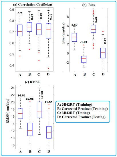
Figure 2.
Performance assessment of 3B42RT and the corrected product during training and testing periods across the Ashti catchment using box plots of (a) correlation coefficient (CC), (b) bias, and (c) root mean square error (RMSE). Bold values in the box plot represent the median values of the statistical measures.
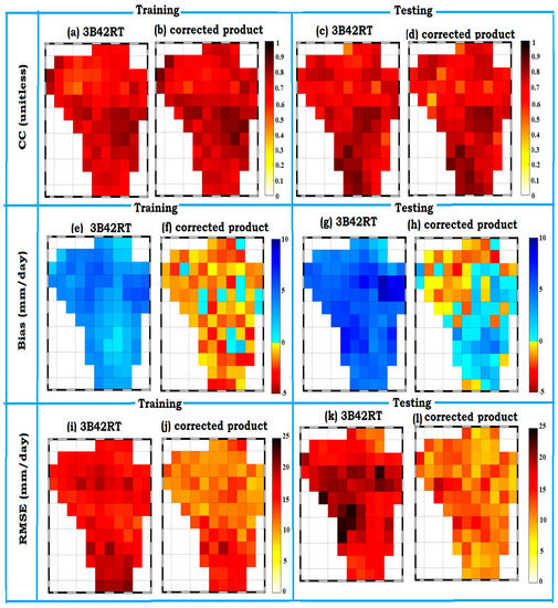
Figure 3.
Spatial distribution of the performance of 3B42RT and the corrected product using CC (a–d), bias (e–h), and RMSE (i–l) during the training and testing periods across the Ashti catchment.
3.2. Performance Assessment Based on Various Rainfall Intensity Classes
The IMD has classified the rainfall amounts into seven different classes based on intensity (mm/day). However, for this study, four classes are defined, i.e., no rainfall (<0.5 mm/day), light rainfall (0.5 to 7.5 mm/day), moderate rainfall (7.5 to 35.5 mm/day), and heavy rainfall (>35.5 mm/day), due to the low number of samples in some of the IMD-defined rainfall classes. Figure 4 presents the box plot of the statistical measures for these four rainfall classes over the training and testing periods. Spatial distribution of the statistical measures for these rainfall intensity classes during training and testing periods are shown in Figures S2 and S3, respectively.
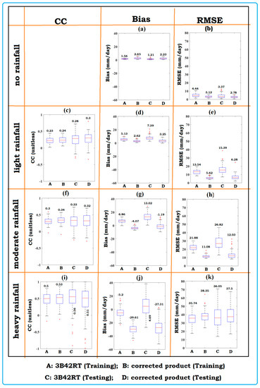
Figure 4.
Performance assessment of 3B42RT and the corrected product for different rainfall intensity classes, i.e., no rainfall (a–b), light rainfall (c–e), moderate rainfall (f–h), and heavy rainfall (i–k) during training and testing periods across the Ashti catchment using box plot of CC, bias and RMSE. Bold values in the box plot represent the median values of the statistical measures.
CC is only reported for three rainfall classes (light rainfall, moderate rainfall, and heavy rainfall) since no rainfall class contains a nil value of the observed IMD rainfall (Figure 4). For the no-rainfall class, 3B42RT shows an overestimation with median bias of 1.56 mm/day (1.21 mm/day) during the training (testing) period, which increased to 2.65 mm/day (2.23 mm/day) in the corrected product (Figure 4a). On the other hand, the median RMSE value in 3B42RT is 4.44 mm/day (3.38 mm/day) during the training (testing) period, which reduced by 29% (17%) in the corrected product (Figure 4b). Along with the box plot, the spatial distribution of RMSE (Figures S2b and S3b) also shows an improvement in the corrected product over 3B42RT across the catchment during training and testing periods. It indicates the improvement occurred throughout the catchment in the corrected product compared to 3B42RT. Note that the Bias is increased, whereas RMSE is decreased in corrected product, as compared to 3B42RT. This indicates a reduction in the random error for the corrected product as compared to 3B42RT, which is consistent with the study carried out by Bhuiyan et al. [44].
With regard to the light and moderate rainfall classes, a marginal improvement in the median value of CC is obtained in the corrected product compared to 3B42RT (Figure 4c,f). On the other hand, the median Bias in 3B42RT is 5.13 mm/day (7.39 mm/day) during the training (testing) period in the light rainfall class, which is drastically reduced by 50% (55%) for the corrected product (Figure 4d). For the moderate rainfall class, it is reduced from 6.86 mm/day (13.02 mm/day) to −4.07 mm/day (−1.19 mm/day) (Figure 4g). Similarly, the median RMSE value of 13.54 mm/day (15.39 mm/day) associated with 3B42RT during the training (testing) period for light rainfall is reduced by 58% (59%) for the corrected product (Figure 4e). For moderate rainfall, it is reduced from 21.88 mm/day (26.82 mm/day) in 3B42RT to 11.08 mm/day (12.03 mm/day) in the corrected product (Figure 4h). Besides these boxplots, the spatial plots also indicate a significant improvement in the bias and RMSE all over the catchment in the corrected product during light and moderate rainfall classes (Figures S2d,e,g,h and S3d,e,g,h). Therefore, a certain improvement in these rainfall classes is observed all over the catchment for the corrected product. The obtained results in these rainfall classes agree with the study carried out by Bhuiyan et al. [44].
For the heavy rainfall class, the median CC value hardly showed any improvement (Figure 4i) in the corrected product over the catchment, which can also be inferred from the spatial distribution maps (Figures S2i and S3i). Some of the grids show CC value near +1 or −1 in Figure S3i, which is due to the presence of very limited samples of heavy rainfall values during the testing period. From Figure 4j–k, it is clear that there is deterioration in the median value of Bias and RMSE in the corrected product as compared to 3B42RT during both training and testing periods. These results are consistent with the work carried out by Bhuiyan et al. [44], and this relatively poor performance may be attributed to fewer samples of heavy rainfall during the model training stage (Refer Figure S4).
In addition to the box plots (Figure 4), to demonstrate the reliability of the correction method, 2-dimensional histograms (Figure 5) along with the value of performance measures (Table 2) are shown for training and testing periods. Data from all the grids in this study (86) are considered in this plot. Overall, a significant scattering in 3B42RT is present along the 1:1 line, which is evidenced by the substantial bias and RMSE (shown in bold values in Figure 5a,c). However, scattering is considerably reduced and samples came near to the 1:1 line in the corrected product, which is reflected by the reduced RMSE and bias in the corrected product (shown in bold values in Figure 5b,d) compared with 3B42RT.
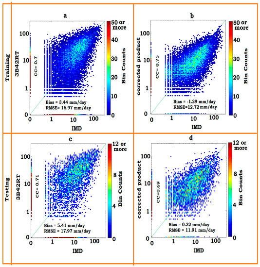
Figure 5.
2-Dimensional histogram of (a,c) 3B42RT versus Indian Meteorological Department (IMD) observed rainfall during training and testing periods; (b,d) corrected product versus IMD observed rainfall during training and testing periods. For better visualization, the rainfall values were plotted on logarithmic scale (with zero values assigned a small positive value of 0.1). The axes report the corresponding rainfall values in linear scale for interpretation purposes. The line of perfect agreement (1:1 line) is also indicated on each plot.
Table 2.
Statistical measures for 3B42RT (corrected product) across various rainfall classes during the training and testing periods.
Regarding intensity-based classes, it can be clearly observed that in the no-rainfall class, positive biases/overestimations are present in 3B42RT in training and testing periods (Figure 5a,c), which is obvious as rainfall cannot be negative. However, these positive biases/overestimations are also present in the corrected product, but with a reduced range of scattering (Figure 5b,d). This is why the RMSE is low in the corrected product for the no-rainfall class (Table 2). During light and moderate rainfall, a notable scattering along the 1:1 line is available in 3B42RT (Figure 5a,c), which introduces considerable biases as well as RMSE during the training and testing periods (Table 2). However, in the corrected product, these are reduced significantly as they approximate to the 1:1 line (Figure 5b,d), thereby reducing the value of bias and RMSE (Table 2). For the heavy rainfall class, scattering along the 1:1 line is not reduced in the corrected product compared to 3B42RT, which is evident from the performance measure (Table 2).
3.3. Performance Assessment Based on Time Series
In this section, the time series plots of IMD gridded rainfall, 3B42RT, and corrected product for the testing period are shown (Figure 6). Out of the 86 grid points enclosing the catchment, three points are selected on the basis of highest, medium, and no improvements of corrected product over 3B42RT (Figure 6a–c). From Figure 6a, it can be observed that 3B42RT shows an overestimation compared to IMD rainfall in most of the testing periods. In contrast, the corrected product is close to the IMD gridded rainfall for most of the testing period. This indicates the corrected product is superior to 3B42RT. However, during heavy rainfall events (more than 35.5 mm/day), the corrected product is not able to reconcile with the IMD gridded rainfall. These results are consistent with the previous results obtained in Section 3.2. Similar findings are also obtained for other grid points considered (Figure 6b,c). It is also evident that the performance of the corrected product (RMSE) deteriorated significantly with the higher frequency and magnitude of heavy rainfall (Figure 6a–c).
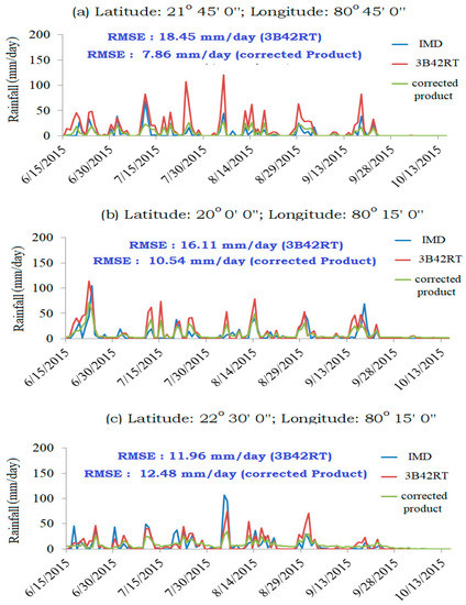
Figure 6.
Time-series of the IMD gridded rainfall, 3B42RT, and the corrected product at grid points having (a) highest (b) medium, and (c) no improvement. For the sake of visualization, only testing periods are shown. Bold values (in Figure 6a–c) represent the RMSE of 3B42RT and the corrected product with respect to IMD gridded rainfall.
4. Summary and Conclusions
In this study, 3B42RT NRT SRE and ASCAT-based NRT soil moisture data are integrated through a machine learning-based SVR model to improve 3B42RT. The statistical measures, i.e., CC, bias, and RMSE, have been chosen to assess the performance. All these performance measures are presented with boxplots and spatial plots. In addition, the time-series plots of IMD, 3B42RT, and the corrected product are also shown to assess the temporal performance of this integration approach.
The obtained results reveal that 3B42RT is associated with significant bias and RMSE. However, in the corrected product, bias and RMSE are significantly reduced compared to 3B42RT rainfall. Particularly, RMSE is decreased by 28% and 33% during the training and testing periods, respectively. With regard to the intensity-based performance, both bias and RMSE are reduced significantly in the corrected product during light and moderate rainfalls over the entire catchment. Even the range of the reduction in RMSE compared with 3B42RT in these two classes is about 50 to 60%. A marginal improvement is also observed in CC values for the corrected product. However, for the heavy rainfall class, no clear improvements are observed, indicating the developed algorithm’s limitation to capture heavy rainfall events. In the no rainfall class, RMSE (bias) is decreased (increased) in the corrected product as compared to 3B42RT, which is due to the improvement in the random error. The obtained results indicate that the proposed approach can effectively reduce the error associated with 3B42RT over Ashti catchment. However, the robustness of the approach needs to be tested rigorously in catchments located in different climatic conditions and using different rainfall products and soil moisture datasets.
Supplementary Materials
The following are available online at https://www.mdpi.com/2072-4292/11/19/2221/s1, Figure S1: Optimum value of the support vector machine-based regression model’s hyperparameters for various grid points across the Ashti catchment. Figure S2: Spatial distribution of the performance of 3B42RT and the corrected product for different rainfall intensity classes, i.e., (a, b) no rainfall; (c–e) light rainfall; (f–h) moderate rainfall; (i–k) heavy rainfall; across the Ashti catchment using CC, bias, and RMSE during the training period. Figure S3. Spatial distribution of the performance of 3B42RT and the corrected product for different rainfall intensity classes, i.e., (a, b) no rainfall; (c–e) light rainfall; (f–h) moderate rainfall; (i–k) heavy rainfall; across the Ashti catchment using CC, bias, and RMSE during the testing period. Figure S4. Number of samples corresponds to various classes of rainfall in 3B42RT and the corrected product during the training and testing periods.
Author Contributions
A.K. and R.R. designed the study. A.K. conducted the analysis and wrote the manuscript. R.R., L.B. and F.M.A. contributed to discussions and revisions of the manuscript, providing important feedback, comments and suggestions.
Funding
This work was funded by Department of Science and Technology (DST), New Delhi under INSPIRE Faculty Award (IFA-12-ENG-36). The article processing charge (APC) was funded by the Robert B. Daugherty Water for Food Global Institute (DWFI), University of Nebraska, Lincoln under the Water Advanced Research and Innovation (WARI) Program, which is supported by the Department of Science and Technology, Government of India, the Indo-US Science and Technology Forum (IUSSTF), the University of Nebraska-Lincoln (UNL).
Acknowledgments
Authors are grateful to Sebastian Hahn, Technische Universität Wien (TU Wien) for his valuable suggestion about Near-Real-Time ASCAT-based soil moisture dataset. We are extending our gratitude to the TRMM and EUMETSAT science teams for making the satellite-based rainfall and soil moisture data available publicly. Also, we are highly thankful to the anonymous reviewers for their constructive comments and suggestions.
Conflicts of Interest
The authors declare no conflict of interest.
References
- Román-Cascón, C.; Pellarin, T.; Gibon, F.; Brocca, L.; Cosme, E.; Crow, W.; Fernández-Prieto, D.; Kerr, Y.H.; Massari, C. Correcting satellite-based precipitation products through SMOS soil moisture data assimilation in two land-surface models of different complexity: API and SURFEX. Remote Sens. Environ. 2017, 200, 295–310. [Google Scholar] [CrossRef]
- Wanders, N.; Pan, M.; Wood, E.F. Correction of real-time satellite precipitation with multi-sensor satellite observations of land surface variables. Remote Sens. Environ. 2015, 160, 206–221. [Google Scholar] [CrossRef]
- Lanza, L.G.; Vuerich, E. The WMO field intercomparison of rain intensity gauges. Atmos. Res. 2009, 94, 534–543. [Google Scholar] [CrossRef]
- Lemma, E.; Upadhyaya, S.; Ramsankaran, R. Investigating the performance of satellite and reanalysis rainfall products at monthly timescales across different rainfall regimes of Ethiopia. Int. J. Remote Sens. 2019, 40, 4019–4042. [Google Scholar] [CrossRef]
- Joyce, R.J.; Janowiak, J.E.; Arkin, P.A.; Xie, P. CMORPH: A method that produces global precipitation estimates from passive microwave and infrared data at high spatial and temporal resolution. J. Hydrometeorol. 2004, 5, 487–503. [Google Scholar] [CrossRef]
- Kubota, T.; Shige, S.; Hashizume, H.; Aonashi, K.; Takahashi, N.; Seto, S.; Hirose, M.; Takayabu, Y.N.; Ushio, T.; Nakagawa, K.; et al. Global precipitation map using satellite-borne microwave radiometers by the GSMaP project: Production and validation. IEEE Trans. Geosci. Remote Sens. 2007, 45, 2259–2275. [Google Scholar] [CrossRef]
- Mishra, A.; Gairola, R.M.; Varma, A.K.; Agarwal, V.K. Remote sensing of precipitation over Indian land and oceanic regions by synergistic use of multisatellite sensors. J. Geophys. Res. Atmos. 2010, 115. [Google Scholar] [CrossRef]
- Prakash, S.; Mahesh, C.; Gairola, R.M.; Pal, P.K. Estimation of Indian summer monsoon rainfall using Kalpana-1 VHRR data and its validation using rain gauge and GPCP data. Meteorol. Atmos. Phys. 2010, 110, 45–57. [Google Scholar] [CrossRef]
- Huffman, G.J.; Bolvin, D.T.; Nelkin, E.J.; Wolff, D.B.; Adler, R.F.; Gu, G.; Hong, Y.; Bowman, K.P.; Stocker, E.F. The TRMM multisatellite precipitation analysis (TMPA): Quasi-global, multiyear, combined-sensor precipitation estimates at fine scales. J. Hydrometeorol. 2007, 8, 38–55. [Google Scholar] [CrossRef]
- Huffman, G.J.; Bolvin, D.T.; Dan, B.; Hsu, K.; Joyce, R.; Kidd, C.; Nelkin, E.J.; Sorooshian, S.; Tan, J.; Xie, P. Algorithm Theoretical Basis Document(ATBD) Version 5.2 NASA Global Precipitation Measurement (GPM) Integrated Multi-Satellite Retrievals for GPM (IMERG); NASA/GSFC: Greenbelt, MD, USA, 2018.
- Beaufort, A.; Gibier, F.; Palany, P. Assessment and correction of three satellite rainfall estimate products for improving flood prevention in French Guiana. Int. J. Remote Sens. 2019, 40, 171–196. [Google Scholar] [CrossRef]
- Bharti, V.; Singh, C.; Ettema, J.; Turkington, T.A.R. Spatiotemporal characteristics of extreme rainfall events over the Northwest Himalaya using satellite data. Int. J. Climatol. 2016, 36, 3949–3962. [Google Scholar] [CrossRef]
- Cai, Y.; Jin, C.; Wang, A.; Guan, D.; Wu, J.; Yuan, F.; Xu, L. Comprehensive precipitation evaluation of TRMM 3B42 with dense rain gauge networks in a mid-latitude basin, northeast, China. Theor. Appl. Climatol. 2016, 126, 659–671. [Google Scholar] [CrossRef]
- Gebere, S.; Alamirew, T.; Merkel, B.; Melesse, A. Performance of high resolution satellite rainfall products over data scarce parts of Eastern Ethiopia. Remote Sens. 2015, 7, 11639–11663. [Google Scholar] [CrossRef]
- Ringard, J.; Becker, M.; Seyler, F.; Linguet, L. Temporal and spatial assessment of four satellite rainfall estimates over French Guiana and North Brazil. Remote Sens. 2015, 7, 16441–16459. [Google Scholar] [CrossRef]
- Tan, M.; Duan, Z. Assessment of GPM and TRMM precipitation products over Singapore. Remote Sens. 2017, 9, 720. [Google Scholar] [CrossRef]
- Chen, S.; Hong, Y.; Gourley, J.J.; Huffman, G.J.; Tian, Y.; Cao, Q.; Yong, B.; Kirstetter, P.-E.; Hardy, J.H.; Li, Z.; et al. Evaluation of the successive V6 and V7 TRMM multisatellite precipitation analysis over the Continental United States. Water Resour. Res. 2013, 49, 8174–8186. [Google Scholar] [CrossRef]
- Hirpa, F.A.; Gebremichael, M.; Hopson, T. Evaluation of high-resolution satellite precipitation products over very complex terrain in Ethiopia. J. Appl. Meteorol. Clim. 2010, 49, 1044–1051. [Google Scholar] [CrossRef]
- Maggioni, V.; Meyers, P.C.; Robinson, M.D. A review of merged high-resolution satellite precipitation product accuracy during the Tropical Rainfall Measuring Mission (TRMM) era. J. Hydrometeorol. 2016, 17, 1101–1117. [Google Scholar] [CrossRef]
- Qin, Y.; Chen, Z.; Shen, Y.; Zhang, S.; Shi, R. Evaluation of satellite rainfall estimates over the Chinese Mainland. Remote Sens. 2014, 6, 11649–11672. [Google Scholar] [CrossRef]
- Yong, B.; Chen, B.; Gourley, J.J.; Ren, L.; Hong, Y.; Chen, X.; Wang, W.; Chen, S.; Gong, L. Intercomparison of the Version-6 and Version-7 TMPA precipitation products over high and low latitudes basins with independent gauge networks: Is the newer version better in both real-time and post-real-time analysis for water resources and hydrologic extremes? J. Hydrol. 2014, 508, 77–87. [Google Scholar]
- Zambrano-Bigiarini, M.; Nauditt, A.; Birkel, C.; Verbist, K.; Ribbe, L. Temporal and spatial evaluation of satellite-based rainfall estimates across the complex topographical and climatic gradients of Chile. Hydrol. Earth Syst. Sci. 2017, 21, 1295–1320. [Google Scholar] [CrossRef]
- Alazzy, A.A.; Lü, H.; Chen, R.; Ali, A.B.; Zhu, Y.; Su, J. Evaluation of satellite precipitation products and their potential influence on hydrological modeling over the Ganzi River Basin of the Tibetan Plateau. Adv. Meteorol. 2017, 2017, 3695285. [Google Scholar] [CrossRef]
- Guo, R.; Liu, Y. Evaluation of satellite precipitation products with rain gauge data at different scales: Implications for hydrological applications. Water 2016, 8, 281. [Google Scholar] [CrossRef]
- Liu, Z. Comparison of precipitation estimates between Version 7 3-hourly TRMM Multi-Satellite Precipitation Analysis (TMPA) near-real-time and research products. Atmos. Res. 2015, 153, 119–133. [Google Scholar] [CrossRef]
- Milewski, A.; Elkadiri, R.; Durham, M. Assessment and comparison of TMPA satellite precipitation products in varying climatic and topographic regimes in Morocco. Remote Sens. 2015, 7, 5697–5717. [Google Scholar] [CrossRef]
- Prakash, S.; Mitra, A.K.; AghaKouchak, A.; Pai, D.S. Error characterization of TRMM Multisatellite Precipitation Analysis (TMPA-3B42) products over India for different seasons. J. Hydrol. 2015, 529, 1302–1312. [Google Scholar] [CrossRef]
- Anjum, M.N.; Ding, Y.; Shangguan, D.; Ijaz, M.W.; Zhang, S. Evaluation of high-resolution satellite-based real-time and post-real-time precipitation estimates during 2010 extreme flood event in Swat River Basin, Hindukush region. Adv. Meteorol. 2016, 2016, 2604980. [Google Scholar] [CrossRef]
- Ren, P.; Li, J.; Feng, P.; Guo, Y.; Ma, Q. Evaluation of multiple satellite precipitation products and their use in hydrological modelling over the Luanhe River basin, China. Water 2018, 10, 677. [Google Scholar] [CrossRef]
- Yong, B.; Ren, L.L.; Hong, Y.; Wang, J.H.; Gourley, J.J.; Jiang, S.H.; Chen, X.; Wang, W. Hydrologic evaluation of Multisatellite Precipitation Analysis standard precipitation products in basins beyond its inclined latitude band: A case study in Laohahe basin, China. Water Resour. Res. 2010, 46. [Google Scholar] [CrossRef]
- Behrangi, A.; Khakbaz, B.; Jaw, T.C.; AghaKouchak, A.; Hsu, K.; Sorooshian, S. Hydrologic evaluation of satellite precipitation products over a mid-size basin. J. Hydrol. 2011, 397, 225–237. [Google Scholar] [CrossRef]
- Shah, R.D.; Mishra, V. Development of an experimental near-real-time drought monitor for India. J. Hydrometeorol. 2015, 16, 327–345. [Google Scholar] [CrossRef]
- Ringard, J.; Seyler, F.; Linguet, L. A quantile mapping bias correction method based on hydroclimatic classification of the Guiana shield. Sensors 2017, 17, 1413. [Google Scholar] [CrossRef] [PubMed]
- Tian, Y.; Peters-Lidard, C.D.; Eylander, J.B. Real-time bias reduction for satellite-based precipitation estimates. J. Hydrometeorol. 2010, 11, 1275–1285. [Google Scholar] [CrossRef]
- Ajaaj, A.A.; Mishra, A.K.; Khan, A.A. Comparison of BIAS correction techniques for GPCC rainfall data in semi-arid climate. Stoch. Environ. Res. Risk Assess. 2016, 30, 1659–1675. [Google Scholar] [CrossRef]
- Chen, J.; Brissette, F.P.; Chaumont, D.; Braun, M. Finding appropriate bias correction methods in downscaling precipitation for hydrologic impact studies over North America. Water Resour. Res. 2013, 49, 4187–4205. [Google Scholar] [CrossRef]
- Gebregiorgis, A.S.; Hossain, F. Understanding the dependence of satellite rainfall uncertainty on topography and climate for hydrologic model simulation. IEEE Trans. Geosci. Remote Sens. 2012, 51, 704–718. [Google Scholar] [CrossRef]
- Maggioni, V.; Sapiano, M.R.; Adler, R.F. Estimating uncertainties in high-resolution satellite precipitation products: Systematic or random error? J. Hydrometeorol. 2016, 17, 1119–1129. [Google Scholar] [CrossRef]
- Pipunic, R.C.; Ryu, D.; Costelloe, J.F.; Su, C.H. An evaluation and regional error modeling methodology for near-real-time satellite rainfall data over Australia. J. Geophys. Res. Atmos. 2015, 120, 10767–10783. [Google Scholar] [CrossRef]
- Yong, B.; Chen, B.; Tian, Y.; Yu, Z.; Hong, Y. Error-component analysis of TRMM-based multi-satellite precipitation estimates over mainland China. Remote Sens. 2016, 8, 440. [Google Scholar] [CrossRef]
- Upadhyaya, S.; Ramsankaran, R. Modified-INSAT Multi-Spectral Rainfall Algorithm (M-IMSRA) at climate region scale: Development and validation. Remote Sens. Environ. 2016, 187, 186–201. [Google Scholar] [CrossRef]
- Yin, Z.Y.; Zhang, X.; Liu, X.; Colella, M.; Chen, X. An assessment of the biases of satellite rainfall estimates over the Tibetan Plateau and correction methods based on topographic analysis. J. Hydrometeorol. 2008, 9, 301–326. [Google Scholar] [CrossRef]
- Yang, Y.; Luo, Y. Using the back propagation neural network approach to bias correct TMPA data in the arid region of Northwest China. J. Hydrometeorol. 2014, 15, 459–473. [Google Scholar] [CrossRef]
- Bhuiyan, M.A.E.; Efthymios, I.; Emmanouil, N. A nonparametric statistical technique for combining global precipitation datasets: Development and hydrological evaluation over the Iberian Peninsula. Hydrol. Earth Syst. Sci. 2018, 1607, 7938. [Google Scholar] [CrossRef]
- Maggioni, V.; Massari, C. On the performance of satellite precipitation products in riverine flood modeling: A review. J. Hydrol. 2018, 558, 214–224. [Google Scholar] [CrossRef]
- Crow, W.T.; Huffman, G.J.; Bindlish, R.; Jackson, T.J. Improving satellite-based rainfall accumulation estimates using spaceborne surface soil moisture retrievals. J. Hydrometeorol. 2009, 10, 199–212. [Google Scholar] [CrossRef]
- Crow, W.T.; van Den Berg, M.J.; Huffman, G.J.; Pellarin, T. Correcting rainfall using satellite-based surface soil moisture retrievals: The Soil Moisture Analysis Rainfall Tool (SMART). Water Resour. Res. 2011, 47. [Google Scholar] [CrossRef]
- Brocca, L.; Ciabatta, L.; Massari, C.; Moramarco, T.; Hahn, S.; Hasenauer, S.; Kidd, R.; Dorigo, W.; Wagner, W.; Levizzani, V. Soil as a natural rain gauge: Estimating global rainfall from satellite soil moisture data. J. Geophys. Res. Atmos. 2014, 119, 5128–5141. [Google Scholar] [CrossRef]
- Han, E.; Merwade, V.; Heathman, G.C. Implementation of surface soil moisture data assimilation with watershed scale distributed hydrological model. J. Hydrol. 2012, 416, 98–117. [Google Scholar] [CrossRef]
- Koster, R.D.; Brocca, L.; Crow, W.T.; Burgin, M.S.; De Lannoy, G.J. Precipitation estimation using L-band and C-band soil moisture retrievals. Water Resour. Res. 2016, 52, 7213–7225. [Google Scholar] [CrossRef]
- Loizu, J.; Massari, C.; Álvarez-Mozos, J.; Tarpanelli, A.; Brocca, L.; Casalí, J. On the assimilation set-up of ASCAT soil moisture data for improving streamflow catchment simulation. Adv. Water Resour. 2018, 111, 86–104. [Google Scholar] [CrossRef]
- Tarpanelli, A.; Massari, C.; Ciabatta, L.; Filippucci, P.; Amarnath, G.; Brocca, L. Exploiting a constellation of satellite soil moisture sensors for accurate rainfall estimation. Adv. Water Resour. 2017, 108, 249–255. [Google Scholar] [CrossRef]
- Hengade, N.; Eldho, T.I. Assessment of LULC and climate change on the hydrology of Ashti Catchment, India using VIC model. J. Earth Syst. Sci. 2016, 125, 1623–1634. [Google Scholar] [CrossRef]
- Das, J.; Nanduri, U.V. Assessment and evaluation of potential climate change impact on monsoon flows using machine learning technique over Wainganga River basin, India. Hydrol. Sci. J. 2018, 63, 1020–1046. [Google Scholar] [CrossRef]
- Central Water Commission. The Godavari River System. Available online: http://www.kgbo-cwc.ap.nic.in/About%20Basins/About%20Godavari%20Basin.pdf (accessed on 10 February 2019).
- Pai, D.S.; Sridhar, L.; Rajeevan, M.; Sreejith, O.P.; Satbhai, N.S.; Mukhopadhyay, B. Development of a new high spatial resolution (0.25 × 0.25) long period (1901–2010) daily gridded rainfall data set over India and its comparison with existing data sets over the region. Mausam 2014, 65, 1–18. [Google Scholar]
- Bharti, V.; Singh, C. Evaluation of error in TRMM 3B42V7 precipitation estimates over the Himalayan region. J. Geophys. Res. Atmos. 2015, 120, 12458–12473. [Google Scholar] [CrossRef]
- Prakash, S.; Mitra, A.K.; Rajagopal, E.N.; Pai, D.S. Assessment of TRMM-based TMPA-3B42 and GSMaP precipitation products over India for the peak southwest monsoon season. Int. J. Climatol. 2016, 36, 1614–1631. [Google Scholar] [CrossRef]
- Prakash, S.; Mitra, A.K.; AghaKouchak, A.; Liu, Z.; Norouzi, H.; Pai, D.S. A preliminary assessment of GPM-based multi-satellite precipitation estimates over a monsoon dominated region. J. Hydrol. 2018, 556, 865–876. [Google Scholar] [CrossRef]
- Hu, Q.; Yang, D.; Wang, Y.; Yang, H. Accuracy and spatio-temporal variation of high resolution satellite rainfall estimate over the Ganjiang River Basin. Sci. China Technol. Sci. 2013, 56, 853–865. [Google Scholar] [CrossRef]
- Maggioni, V.; Vergara, H.J.; Anagnostou, E.N.; Gourley, J.J.; Hong, Y.; Stampoulis, D. Investigating the applicability of error correction ensembles of satellite rainfall products in river flow simulations. J. Hydrometeorol. 2013, 14, 1194–1211. [Google Scholar] [CrossRef]
- Mei, Y.; Anagnostou, E.N.; Nikolopoulos, E.I.; Borga, M. Error analysis of satellite precipitation products in mountainous basins. J. Hydrometeorol. 2014, 15, 1778–1793. [Google Scholar] [CrossRef]
- Pipunic, R.; Ryu, D.; Costelloe, J.; Su, C.H. Evaluation of real-time satellite rainfall products in semi-arid/arid Australia. In Proceedings of the 20th International Congress on Modelling and Simulation, Adelaide, Australia, 1–6 December 2013; pp. 3106–3112. [Google Scholar]
- Schwaller, M.R.; Morris, K.R. A ground validation network for the global precipitation measurement mission. J. Atmos. Ocean. Tech. 2011, 28, 301–319. [Google Scholar] [CrossRef]
- Naeimi, V.; Scipal, K.; Bartalis, Z.; Hasenauer, S.; Wagner, W. An improved soil moisture retrieval algorithm for ERS and METOP scatterometer observations. IEEE Trans. Geosci. Remote Sens. 2009, 47, 1999–2013. [Google Scholar] [CrossRef]
- Wagner, W.; Lemoine, G.; Borgeaud, M.; Rott, H. A study of vegetation cover effects on ERS scatterometer data. IEEE Trans. Geosci. Remote Sens. 1999, 37, 938–948. [Google Scholar] [CrossRef]
- Brocca, L.; Crow, W.T.; Ciabatta, L.; Massari, C.; De Rosnay, P.; Enenkel, M.; Hahn, S.; Amarnath, G.; Camici, S.; Tarpanelli, A.; et al. A review of the applications of ASCAT soil moisture products. IEEE J. Sel. Top. Appl. Earth Obs. Remote Sens. 2017, 10, 2285–2306. [Google Scholar] [CrossRef]
- Brocca, L.; Moramarco, T.; Melone, F.; Wagner, W.; Hasenauer, S.; Hahn, S. Assimilation of surface-and root-zone ASCAT soil moisture products into rainfall–runoff modeling. IEEE Trans. Geosci. Remote Sens. 2012, 50, 2542–2555. [Google Scholar] [CrossRef]
- Massari, C.; Brocca, L.; Tarpanelli, A.; Moramarco, T. Data assimilation of satellite soil moisture into rainfall-runoff modelling: A complex recipe? Remote Sens. 2015, 7, 11403–11433. [Google Scholar] [CrossRef]
- Product User Manual Surface Soil Moisture ASCAT NRT Orbit. 2016. Available online: http://hsaf.meteoam.it/documents/PUM/ssm_ascat_nrt_o_pum.pdf (accessed on 1 March 2019).
- EUMETSAT. Available online: https://eoportal.eumetsat.int/userMgmt/login.faces (accessed on 12 March 2019).
- Brocca, L.; Hasenauer, S.; Lacava, T.; Melone, F.; Moramarco, T.; Wagner, W.; Dorigo, W.; Matgen, P.; Martínez-Fernández, J.; Llorens, P.; et al. Soil moisture estimation through ASCAT and AMSR-E sensors: An intercomparison and validation study across Europe. Remote Sens. Environ. 2011, 115, 3390–3408. [Google Scholar] [CrossRef]
- Wagner, W.; Hahn, S.; Kidd, R.; Melzer, T.; Bartalis, Z.; Hasenauer, S.; Figa-Saldaña, J.; de Rosnay, P.; Jann, A.; Schneider, S.; et al. The ASCAT soil moisture product: A review of its specifications, validation results, and emerging applications. Meteorol. Z. 2013, 22, 5–33. [Google Scholar] [CrossRef]
- Asefa, T.; Kemblowski, M.; McKee, M.; Khalil, A. Multi-time scale stream flow predictions: The support vector machines approach. J. Hydrol. 2006, 318, 7–16. [Google Scholar] [CrossRef]
- Shamshirband, S.; Petković, D.; Amini, A.; Anuar, N.B.; Nikolić, V.; Ćojbašić, Ž.; Kiah, M.L.M.; Gani, A. Support vector regression methodology for wind turbine reaction torque prediction with power-split hydrostatic continuous variable transmission. Energy 2014, 67, 623–630. [Google Scholar] [CrossRef]
- Kalra, A.; Ahmad, S. Estimating annual precipitation for the Colorado River Basin using oceanic-atmospheric oscillations. Water Resour. Res. 2012, 48. [Google Scholar] [CrossRef]
- Sudheer, C.; Maheswaran, R.; Panigrahi, B.K.; Mathur, S. A hybrid SVM-PSO model for forecasting monthly streamflow. Neural Comput. Appl. 2014, 24, 1381–1389. [Google Scholar] [CrossRef]
- Himanshu, S.K.; Pandey, A.; Yadav, B. Assessing the applicability of TMPA-3B42V7 precipitation dataset in wavelet-support vector machine approach for suspended sediment load prediction. J. Hydrol. 2017, 550, 103–117. [Google Scholar] [CrossRef]
- Khwairakpam, E.; Khosa, R.; Gosain, A.; Nema, A.; Mathur, S.; Yadav, B. Modeling Simulation of River Discharge of Loktak Lake Catchment in Northeast India. J. Hydrol. Eng. 2018, 23, 05018014. [Google Scholar] [CrossRef]
- Yadav, B.; Eliza, K. A hybrid wavelet-support vector machine model for prediction of lake water level fluctuations using hydro-meteorological data. Measurement 2017, 103, 294–301. [Google Scholar] [CrossRef]
- Vapnik, V. The Nature of Statistical Learning Theory, 2nd ed.; Springer: New York, NY, USA, 2000. [Google Scholar]
- Bishop, C.M. Pattern Recognition and Machine Learning; Springer: New York, NY, USA, 2006. [Google Scholar]
- Lima, A.R.; Cannon, A.J.; Hsieh, W.W. Nonlinear regression in environmental sciences by support vector machines combined with evolutionary strategy. Comput. Geosci. 2013, 50, 136–144. [Google Scholar] [CrossRef]
- Vapnik, V.; Golowich, S.E.; Smola, A.J. Support vector method for function approximation, regression estimation and signal processing. In Advances in Neural Information Processing Systems 9; Mozer, M., Jordan, M., Petsche, T., Eds.; MIT Press: Cambridge, MA, USA, 1997. [Google Scholar]
- Xu, T.; Valocchi, A.J. Data-driven methods to improve baseflow prediction of a regional groundwater model. Comput. Geosci. 2015, 85, 124–136. [Google Scholar] [CrossRef]
- Ahmad, S.; Kalra, A.; Stephen, H. Estimating soil moisture using remote sensing data: A machine learning approach. Adv. Water Resour. 2010, 33, 69–80. [Google Scholar] [CrossRef]
- Bray, M.; Han, D. Identification of support vector machines for runoff modelling. J. Hydroinform. 2004, 6, 265–280. [Google Scholar] [CrossRef]
- Yu, P.S.; Chen, S.T.; Chang, I.F. Support vector regression for real-time flood stage forecasting. J. Hydrol. 2006, 328, 704–716. [Google Scholar] [CrossRef]
- Zakaria, Z.A.; Shabri, A. Streamflow forecasting at ungaged sites using support vector machines. Appl. Math. Sci. 2012, 6, 3003–3014. [Google Scholar]
- ASCE. Task Committee on Application of Artificial Neural Networks in Hydrology. Artificial neural networks in hydrology. I: Preliminary concepts. J. Hydrol. Eng. 2000, 5, 115–123. [Google Scholar] [CrossRef]
- Behzad, M.; Asghari, K.; Coppola, E.A., Jr. Comparative study of SVMs and ANNs in aquifer water level prediction. J. Comput. Civ. Eng. 2009, 24, 408–413. [Google Scholar] [CrossRef]
- Karran, D.J.; Morin, E.; Adamowski, J. Multi-step streamflow forecasting using data-driven non-linear methods in contrasting climate regimes. J. Hydroinform. 2014, 16, 671–689. [Google Scholar] [CrossRef]
- Yoon, H.; Jun, S.C.; Hyun, Y.; Bae, G.O.; Lee, K.K. A comparative study of artificial neural networks and support vector machines for predicting groundwater levels in a coastal aquifer. J. Hydrol. 2011, 396, 128–138. [Google Scholar] [CrossRef]
- Yoon, H.; Kim, Y.; Ha, K.; Lee, S.H.; Kim, G.P. Comparative evaluation of ANN-and SVM-time Series models for predicting freshwater-saltwater interface fluctuations. Water 2017, 9, 323. [Google Scholar] [CrossRef]
- Yang, T.; Asanjan, A.A.; Welles, E.; Gao, X.; Sorooshian, S.; Liu, X. Developing reservoir monthly inflow forecasts using artificial intelligence and climate phenomenon information. Water Resour. Res. 2017, 53, 2786–2812. [Google Scholar] [CrossRef]
- Bhagwat, P.P.; Maity, R. Hydroclimatic streamflow prediction using least square-support vector regression. ISH. J. Hydraul. Eng. 2013, 19, 320–328. [Google Scholar] [CrossRef]
- Wang, W.C.; Chau, K.W.; Cheng, C.T.; Qiu, L. A comparison of performance of several artificial intelligence methods for forecasting monthly discharge time series. J. Hydrol. 2009, 374, 294–306. [Google Scholar] [CrossRef]
- Wu, C.L.; Chau, K.W.; Li, Y.S. River stage prediction based on a distributed support vector regression. J. Hydrol. 2008, 358, 96–111. [Google Scholar] [CrossRef]
- Chang, C.; Lin, C. LIBSVM: A Library for Support Vector Machines. ACM Trans. Intell. Syst. Technol. 2012, 2, 27. [Google Scholar] [CrossRef]
- Sunilkumar, K.; Narayana Rao, T.; Saikranthi, K.; Purnachandra Rao, M. Comprehensive evaluation of multisatellite precipitation estimates over India using gridded rainfall data. J. Geophys. Res. Atmos. 2015, 120, 8987–9005. [Google Scholar] [CrossRef]
- Nanda, T.; Sahoo, B.; Beria, H.; Chatterjee, C. A wavelet-based non-linear autoregressive with exogenous inputs (WNARX) dynamic neural network model for real-time flood forecasting using satellite-based rainfall products. J. Hydrol. 2016, 539, 57–73. [Google Scholar] [CrossRef]
- Rasouli, K.; Hsieh, W.W.; Cannon, A.J. Daily streamflow forecasting by machine learning methods with weather and climate inputs. J. Hydrol. 2012, 414, 284–293. [Google Scholar] [CrossRef]
- Yin, Z.Y.; Liu, X.; Zhang, X.; Chung, C.F. Using a geographic information system to improve Special Sensor Microwave Imager precipitation estimates over the Tibetan Plateau. J. Geophys. Res. Atmos. 2004, 109. [Google Scholar] [CrossRef]
- Craney, T.A.; Surles, J.G. Model-dependent variance inflation factor cutoff values. Qual. Eng. 2002, 14, 391–403. [Google Scholar] [CrossRef]
- Hair, J.F.; Black, W.C.; Babin, B.J.; Anderson, R.E. Multivariate Data Analysis: Pearson New International Edition, 7th ed.; Pearson/Prentice Hall: Upper Saddle River, NJ, USA, 2014. [Google Scholar]
- Yu, H.; Jiang, S.; Land, K.C. Multicollinearity in hierarchical linear models. Soc. Sci. Res. 2015, 53, 118–136. [Google Scholar] [CrossRef]
- Suryanarayana, C.; Sudheer, C.; Mahammood, V.; Panigrahi, B.K. An integrated wavelet-support vector machine for groundwater level prediction in Visakhapatnam, India. Neurocomputing 2014, 145, 324–335. [Google Scholar] [CrossRef]
- Yadav, B.; Ch, S.; Mathur, S.; Adamowski, J. Discharge forecasting using an online sequential extreme learning machine (OS-ELM) model: A case study in Neckar River, Germany. Measurement 2016, 92, 433–445. [Google Scholar] [CrossRef]
- Yu, X.; Liong, S.Y.; Babovic, V. EC-SVM approach for real-time hydrologic forecasting. J. Hydroinform. 2004, 6, 209–223. [Google Scholar] [CrossRef]
- Tripathi, S.; Srinivas, V.V.; Nanjundiah, R.S. Downscaling of precipitation for climate change scenarios: A support vector machine approach. J. Hydrol. 2006, 330, 621–640. [Google Scholar] [CrossRef]
- Zhao, W.; Tao, T.; Zio, E. System reliability prediction by support vector regression with analytic selection and genetic algorithm parameters selection. Appl. Soft Comput. 2015, 30, 792–802. [Google Scholar] [CrossRef]
- Yadav, B.; Mathur, S. River discharge simulation using variable parameter McCarthy—Muskingum and wavelet-support vector machine methods. Neural Comput. Appl. 2018, 31, 1–14. [Google Scholar] [CrossRef]
- Lin, J.Y.; Cheng, C.T.; Chau, K.W. Using support vector machines for long-term discharge prediction. Hydrol. Sci. J. 2006, 51, 599–612. [Google Scholar] [CrossRef]
- Raje, D.; Mujumdar, P.P. A comparison of three methods for downscaling daily precipitation in the Punjab region. Hydrol. Process. 2011, 25, 3575–3589. [Google Scholar] [CrossRef]
- Maity, R.; Bhagwat, P.P.; Bhatnagar, A. Potential of support vector regression for prediction of monthly streamflow using endogenous property. Hydrol. Process. 2010, 24, 917–923. [Google Scholar] [CrossRef]
- Baydaroğlu, Ö.; Koçak, K. SVR-based prediction of evaporation combined with chaotic approach. J. Hydrol. 2014, 508, 356–363. [Google Scholar] [CrossRef]
- Ch, S.; Anand, N.; Panigrahi, B.K.; Mathur, S. Streamflow forecasting by SVM with quantum behaved particle swarm optimization. Neurocomputing 2013, 101, 18–23. [Google Scholar] [CrossRef]
- Liu, S.; Tai, H.; Ding, Q.; Li, D.; Xu, L.; Wei, Y. A hybrid approach of support vector regression with genetic algorithm optimization for aquaculture water quality prediction. Math. Comput. Model. 2013, 58, 458–465. [Google Scholar] [CrossRef]
- Camici, S.; Ciabatta, L.; Massari, C.; Brocca, L. How reliable are satellite precipitation estimates for driving hydrological models: A verification study over the Mediterranean area. J. Hydrol. 2018, 563, 950–961. [Google Scholar] [CrossRef]
- Upadhyaya, S.; Ramsankaran, R. Comprehensive inter-comparison of INSAT multispectral rainfall algorithm estimates and TMPA 3B42-RT V7 estimates across different climate regions of India during southwest monsoon period. Environ. Monit. Assess. 2018, 190, 45. [Google Scholar] [CrossRef]
- Yuan, F.; Wang, B.; Shi, C.; Cui, W.; Zhao, C.; Liu, Y.; Ren, L.; Zhang, L.; Zhu, Y.; Chen, T.; et al. Evaluation of hydrological utility of IMERG Final run V05 and TMPA 3B42V7 satellite precipitation products in the Yellow River source region, China. J. Hydrol. 2018, 567, 696–711. [Google Scholar] [CrossRef]


© 2019 by the authors. Licensee MDPI, Basel, Switzerland. This article is an open access article distributed under the terms and conditions of the Creative Commons Attribution (CC BY) license (http://creativecommons.org/licenses/by/4.0/).