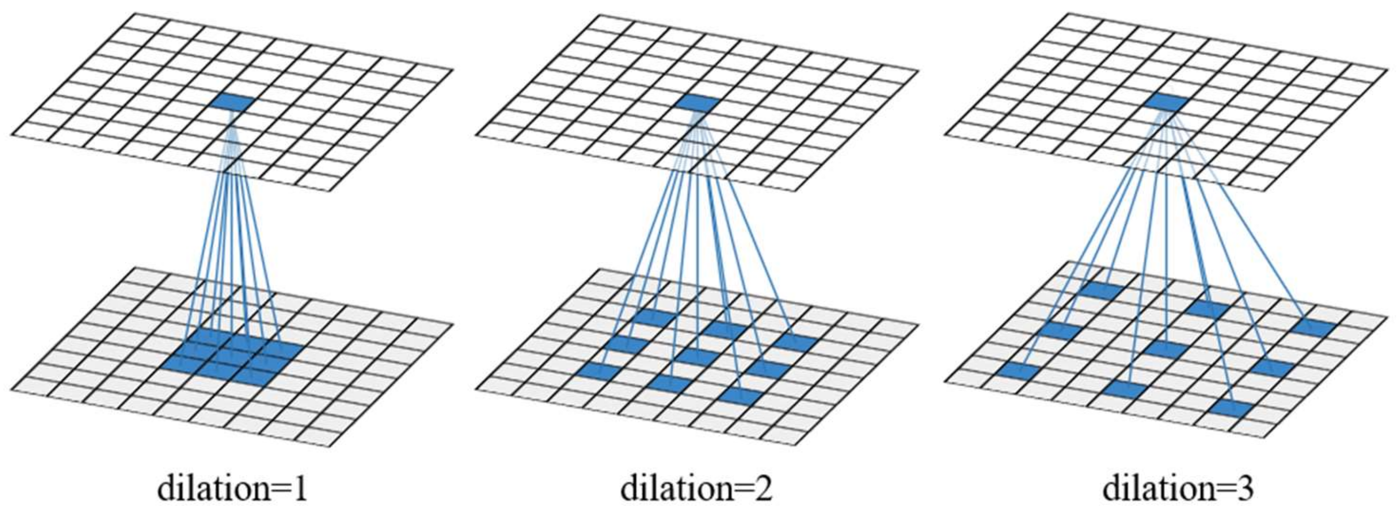
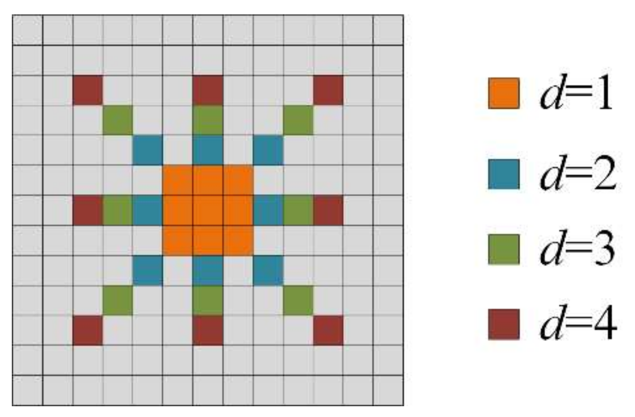
Article

Multiscale Spatial-Spectral Convolutional Network with Image-Based Framework for Hyperspectral Imagery Classification

1
College of Geoscience and Surveying Engineering, China University of Mining and Technology (Beijing), Beijing 100083, China
2
Key Laboratory of Digital Earth Science, Aerospace Information Research Institute, Chinese Academy of Sciences, Beijing 100094, China
3
College of Resources and Environment, University of Chinese Academy of Sciences, Beijing 100049, China
4
Institute of Spacecraft System Engineering (CAST), No.104 Youyi Road, Haidian, Beijing 100094, China
5
Strathclyde Hyperspectral Imaging Centre, Department of Electronic and Electrical Engineering, University of Strathclyde, Glasgow G1 1XQ, UK
*
Author to whom correspondence should be addressed.
Remote Sens. 2019, 11(19), 2220; https://doi.org/10.3390/rs11192220
Submission received: 5 September 2019 / Revised: 5 September 2019 / Accepted: 17 September 2019 / Published: 23 September 2019

Abstract

:
Jointly using spatial and spectral information has been widely applied to hyperspectral image (HSI) classification. Especially, convolutional neural networks (CNN) have gained attention in recent years due to their detailed representation of features. However, most of CNN-based HSI classification methods mainly use patches as input classifier. This limits the range of use for spatial neighbor information and reduces processing efficiency in training and testing. To overcome this problem, we propose an image-based classification framework that is efficient and straightforward. Based on this framework, we propose a multiscale spatial-spectral CNN for HSIs (HyMSCN) to integrate both multiple receptive fields fused features and multiscale spatial features at different levels. The fused features are exploited using a lightweight block called the multiple receptive field feature block (MRFF), which contains various types of dilation convolution. By fusing multiple receptive field features and multiscale spatial features, the HyMSCN has comprehensive feature representation for classification. Experimental results from three real hyperspectral images prove the efficiency of the proposed framework. The proposed method also achieves superior performance for HSI classification.

1. Introduction

Hyperspectral image (HSI) has attracted a lot of attention in recent years since it has hundreds of continuous observation bands throughout the electromagnetic spectrum, ranging from visible to near-infrared wavelengths. HSI has also been used in many applications due to its high-dimensionality and distinct spectral features [1,2,3]. Supervised classification is one of the most critical applications and is widely used in remote sensing. However, spectral-based classification methods typically only measure the spectral characteristics of objects and ignore spatial neighborhood information [4]. Hyperspectral image classification (HSIC) can be improved by considering both spatial and spectral information [5]. Moreover, the multiscale spatial-spectral classification method is well adapted for HSI since different scale regions contain complementary but interconnected information for classification.
Multiscale spatial-spectral classification methods can be categorized into two groups: multiscale superpixel segmentation [6,7,8,9] and multiscale image cubes [10,11,12,13,14,15]. Numerous methods have been developed to determine the optimal scale in multiscale superpixel segmentation. Yu et al. [6] proposed a multiscale superpixel-level support vector machine (SVM) classification method to exploit the spatial information within different superpixel scales. Zhang et al. [7] applied a multiscale superpixel-based sparse representation algorithm to obtain spatial structure information for different segmentation scales and generated a classification map using a sparse representation classifier. Similarly, Dundar et al. [8] added a guided filter to process the first three principal components and implemented multiscale superpixel segmentation. Chen et al. [9] used multiscale segmentation to obtain the spatial information from different levels, and the results of multiscale segmentation were treated as the input for a rotation forest classifier. Finally, the majority voting rule was used to combine the classification results from different segmentation scales.
An image pyramid refers to an image that is subject to repeated smoothing and subsampling and generates a series of weighted down images [10]. Li et al. [11] proposed a segmented principal component analysis and Gaussian pyramid decomposition-based multiscale feature fusion algorithm for HSIC. The Gaussian image pyramid was used to generate images with multiple spatial sizes following PCA dimension reduction. Fang et al. [12] applied a multiscale adaptive sparse representation for selecting the optimal regional scales for different HSIs with various structures. Liu et al. [13] proposed a multiscale representation based on random projection. This method modeled the spatial characteristics at all reasonable scales comprising each pixel and its neighbors. A multiscale joint collaborative representation with a locally adaptive dictionary was developed to incorporate complementary contextual information into classification by multiplying different scales with distinct spatial structures and characteristics [14]. He et al. [15] proposed feature extraction with a multiscale covariance map for HSIC. In their work, a series of multiscale cubes were constructed for each pixel in the dimension-reduced imagery. A Gaussian pyramid and edge-preserving filtering were also used to extract multi-scale features. The final classification map was produced using a majority voting method [16]. Most of these multiscale classification methods independently extract features or spatial structures at different image scales and fuse the classification results in the final prediction stage. Thus, there is no interaction between the features at different scales.
Deep learning-based models have also been introduced for the HSIC in recent years. Spatial-spectral features can be extracted using a deep convolutional neural network, and these features represent low-to-high level semantic information. Different deep learning architectures have also been introduced for HSIC [17,18,19,20,21,22,23]. Li et al. [17] proposed a pixel-pair method to significantly increase the number of training samples. This was necessary to overcome the imbalance between the high dimensionality of spectral features and limited training samples (also known as the Hughes phenomenon). A similar cube-pair 3-D convolution neural network (CNN) classification model has also been proposed [18]. Du et al. proposed an unsupervised network to extract high-level feature representations without any label information [19]. Recurrent neural network (RNN) and parametric rectified tanh activation functions have been introduced for HSIC [20]. Self-taught learning was used for unsupervised extraction of features from unlabeled HSI [21]. Lee et al. [22] proposed a network to extract features with multiple convolution filter sizes. Residual connection and 3-D convolution have also been applied to HSIC [23], and semi-supervised classification methods have been developed as well [24,25,26]. He et al. [24] proposed a semi-supervised model using generative adversarial networks (GAN) to use the limited labeled samples for HSIC. A multi-channel network was proposed to extract the joint spectral-spatial features using semi-supervised classification [25]. Zhan et al. [26] developed 1-D GAN to generate hyperspectral samples that were similar to real spectral vectors. Ahmad et. al [27] proposed a semi-supervised multi-kernel class consistency regularizer graph-based spatial-spectral feature learning framework.
More recently, various convolution neural networks with multiscale spatial-spectral features have been introduced for hyperspectral image classification [28,29,30,31,32,33,34,35,36,37,38,39,40,41]. Jiao et al. [28] used a pooling operation to generate multiple images from HSI, and a pretrained VGG-16 was introduced to extract multiscale features. Fusion features were then fed into classifiers. Liang et al. [29] also used pretrained VGG-16 to extract multiscale spatial structures and proposed an unsupervised cooperative sparse autoencoder method to fuse deep spatial features and spectral information. Multiscale feature extraction has also been proposed using multiple convolution kernel sizes and determinantal point process priors [30]. An automatic design CNN was introduced with automatic 1-D Auto-CNN and 3-D Auto-CNN [31]. An attention mechanism was also introduced for HSIC [32,33,34]. Fang et al. [32] proposed a 3-D dense convolutional network with a spectral attention network. Wang et al. [33] designed a spatial-spectral squeeze-and-excitation residual network to exploit the attention mechanism for HSIC. Mei et al. [34] used RNN and CNN to design a two-branch spatial-spectral attention network. Zhang et al. [35] proposed 3-D lightweight CNN for limited training samples and also presented two transfer learning strategies: (1) cross-sensor strategy and (2) cross-modal strategy. An unsupervised spatial-spectral feature learning strategy was proposed using 3-D CNN autoencoder to learn effective spatial-spectral features [36]. A multiscale deep middle-level feature fusion network was proposed to consider the complementary and related information among different scale features [37]. Two convolution capsule networks were proposed to enrich the spatial-spectral features [38,39]. Pan et. al [40] proposed rolling guidance filter and vertex component analysis network to utilize spatial-spectral information. Several other CNN-based HSIC methods were also proposed [41,42,43]. However, some of these multiscale methods still focus on independently extracting multiscale features based on different image scales. Most importantly, these methods only use image patches as model inputs, which limits the understanding of the remote sensing image.
This paper proposes an image-based classification framework for HSI to address the inefficient performance of existing methods. Based on this framework, this paper proposes a novel HyMSCN (Multiscale Spatial-spectral Convolutional Network for Hyperspectral Image) network to improve the representation ability for HSI. The main contribution of the proposed approach can be summarized as follows:
(1)
A novel image-based classification framework is proposed for hyperspectral image classification. The proposed framework is more universal, efficient, and straightforward for training and testing processes compared to the traditional patch-based framework.
(2)
Local neighbor spatial information is exploited using a residual multiple receptive field fusion block (ReMRFF). This block integrates residual learning and multiple dilated convolutions featured as lightweight and efficient feature extraction.
(3)
Multiscale spatial-spectral features are exploited using the proposed HyMSCN method. The method is based on the feature pyramid structure and considers both multiple receptive field fused features and multiscale spatial features at different levels. This approach allows for comprehensive feature representation.
The remainder of this paper is organized as follows. Section 2 introduces the dilation convolution and the feature pyramid. Section 3 presents the details of the proposed classification framework and HyMSCN. Section 4 evaluates the performances of our method compared with those of other hyperspectral image classifiers. Section 5 provides a discussion of the results, and the conclusion is presented in Section 6.

2. Related Works

2.1. Dilated Convolution

Dilated convolution, or atrous convolution, has been shown to be effective for semantic segmentation [44,45,46,47]. The dilated convolution refers to “convolution with a dilated filter”, and the operator of dilated convolution can apply the same filter at different ranges using different dilation factors [44]. It is likely constructed by inserting holes between each pixel in the convolution kernel. The operation of one 3×3 dilated convolution with different dilation factors is shown in Figure 1. It can be found that the dilation factor decides the sampling distance of the convolution kernel. Naturally, the extracted features represent spatial structure information at different scales. A larger convolution kernel can be used to enlarge the receptive field (such as 5×5 or 7×7). However, the number of parameters should be small to prevent overfitting since HSI contains a small number of training samples [5]. Dilated convolution can enlarge the receptive field with the same number of parameters, and is well adapted for HSIC.
A “gridding problem” is known to exist in the dilated convolution framework [44,45]. This can result in serration gridding, as shown in Figure 2. Wang et al. [46] addressed this problem by developing a hybrid dilated convolution (HDC) to choose a series of proper dilation factors to avoid gridding. Chen et al. [45,47] proposed atrous spatial pyramid pooling (ASPP) to exploit multiscale features by employing multiple parallel filters with different dilation factors. The main purpose of both methods is to ensure that the final size of the receptive field fully covers a square region without any holes or missing edges. Following their work, we also designed a lightweight dilated convolution block to fuse multiple receptive field features (see Section 3.2).

2.2. Feature Pyramid

Most hyperspectral image classification methods [11,14,15,16,28,29] construct image pyramids to extract multiscale features, such as in Figure 3a. These features are independently extracted for each image scale, which is a slow process. Most importantly, the image pyramid suffers from a deficiency in semantic classification and lacks interaction between different feature scales.
The feature pyramid network was first proposed by Lin et al. [48] for object detection. The method is developed to detect objects at different scales. Multiscale features enable the model to obtain a large range of scales at different pyramid levels for segmentation. A convolution network can extract hierarchical features layer by layer, and a convolution layer with a stride greater than one can change the feature spatial size to construct inherent multiscale features within a pyramid (Figure 3b). The feature pyramid produces multiscale features with strong semantic representation even at high-resolution feature scales. Additionally, the architecture combines low-to-high level features with top-down feature fusion which has rich semantics at all levels [48]. The hyperspectral image classification network was designed based on this strategy (see Section 3.3).

3. Proposed Methods

In this section, we propose an image-based framework for HSI that has greater flexibility and efficiency compared with the tradition patch-based classification framework (see Section 3.1). A novel multiscale spatial-spectral convolutional network, or HyMSCN, was developed based on this framework. The network is composed of two components, including a residual multiple receptive field fusion block (ResMRFF) and feature pyramid. ResMRFF mainly focuses on extracting multiple receptive field features with lightweight parameters to avoid overfitting (see Section 3.2). In Section 3.3, the network structure containing the feature pyramid is developed and used to extract multiple features that have strong semantics at different scales. The multiscale features are then fused for the final classification.

3.1. Patch-Based Classification and Image-Based Classification for HSI

Most deep learning-based hyperspectral image classification methods generate image patches as training data to extract spatial-spectral information. This is known as a patch-based classification for hyperspectral imagery. The patch-based classification framework is displayed in Figure 4. The training pixel and its neighbor pixels are selected as training patches. These patches are fed into the model to predict the labels for the center pixel of each patch. This method is observed to generate patches pixel by pixel during testing. Patches are then inputted into the model one by one and finally reshapes the predicted labels to the spatial size of the input image.
Obviously, the patch-based classification method has several disadvantages. Firstly, the patch size restricts the receptive field of the classification model. In CNN-based hyperspectral image classification models, the model cannot obtain information larger than the patch size even though the model is composed of a series of 3×3 convolution layers. Secondly, the model must be redesigned if the patch size changes. Most importantly, the optimal patch size is decided by the ground sample distance (GSD) of a remote sensing image. It is difficult to design a universal patch-based model to fit arbitrary images. Thirdly, the pixel-by-pixel processing of the test phase is inefficient. The testing patches will consume more memory than the original image because of the redundant information between different patches. In addition, for CNN-based model, the testing process with one by one processing will consume more bandwidth in the central processing unit (CPU) and graphics processing unit (GPU).
In this study, we propose an image-based classification framework as an alternative to overcome the above issues associated with patch-based classification (Figure 5). The image-based framework can utilize an arbitrary semantic segmentation model for hyperspectral image classification. Due to the fact that only a small number of pixels with labeled information can be used for training in HSIC. The training phase is different from the one of semantic segmentation model used in computer vision [34,35,36]. In training phase, the image containing training samples is used as the input, and the output is the predicted labels for all corresponding pixels. Since only part of pixels in this image has labels, the position of labeled samples acting as a mask covers the output to select the corresponding pixels. The loss is calculated between the selected pixels and labeled pixels. In testing phase, an image is used as input and the corresponding labels are predicted for all the pixels. The image-based classification framework can fully utilize the graphics processing unit during testing to accelerate the inference process with non-redundant information. Moreover, the receptive field is not affected by the patch size since there is no slicing operation, and the testing process is simple and straightforward. This can directly output the results of the test image in one inference instead of pixel-by-pixel processing each patch. This will save more computing resources than the patch-based classification framework.

3.2. Residual Multiple Receptive Field Fusion Block

The residual block is a popular CNN structure used in many computer vision tasks [49,50]. The method uses a skip connection to construct identity mapping which enables the block to learn the residual function. The residual function can be formulated as: Xi=f(Xi-1)+Xi-1, where Xi-1 and Xi refer to the input and output of one residual block and f(⋅) refers to the non-linear transformation. A typical illustration of the residual block is shown in Figure 6. This method suggests that the forward and backward signals can be directly propagated from one residual block to another block. This can enhance the gradient transfer from top to bottom of the network and mitigate the gradient disappearance in the deep network.
Following the strategy of the residual block, we designed a new block called ResMRFF which consists of residual learning and multiple receptive field fusion block (MRFF). In the new block, MRFF is used to replace the convolution layer of the original residual block to enlarge the receptive field with fewer parameters. MRFF is designed to enlarge the receptive field of features with fewer parameters based on the dilation convolution (Figure 7). The structure is designed following the reduce-transform-merge strategy. Firstly, a 1×1 convolution layer is used to reduce feature dimension. Secondly, dilation convolution layers are used to extract features with a variety of dilation factors. Lastly, multiple features are fused using a hierarchical feature fusion strategy [51]. Larger receptive field features are fused with smaller receptive field features to improve representation at different spatial ranges.
Due to only a small number of labeled samples are available in HSIC, it is reasonable to reduce the number of parameters to avoid overfitting. For an input feature X i 1 R H i n × W i n × C i n , a standard convolution layer contains Cout kernels k R k × k × C i n to produce output feature X i R H o u t × W o u t × C o u t . H, W, C, and k represent the height and width of the features, channels, and kernel sizes, respectively. The number of parameters is Cin×k×k×Cout for a standard convolution layer. The MRFF module is designed to follow the reduce-transform-merge strategy to reduce the number of parameters and to make the network more computationally efficient [52,53,54]. Firstly, a 1×1 convolution layer is introduced to reduce the feature dimension by a factor of 4. Secondly, dilated convolution layers with different dilation factors are utilized to obtain multiple spatial features in parallel. Finally, multiple spatial features are fused using a 1×1 convolution layer with a hierarchical feature fusion strategy. The MRFF module is thus stated to have ( C i n ) 2 / 4 + ( k C i n ) 2 / 4 + C i n C o u t parameters. Conversely, a standard convolution has Cin×k×k×Cout parameters. Generally, the MRFF has fewer parameters and this enables the module to be faster and more efficient.
Additionally, MRFF can obtain multiple receptive field features. A standard convolution layer has a k × k receptive field. Conversely, the receptive field of one dilated convolution layer is (k−1)d+1, where k and d refer to kernel size and dilation factor. In our MRFF module, four different dilation factors (1,2,3,4) are used and the receptive field of merged features is similar to Figure 8. MRFF employs multiple dilated convolutions to enlarge the diversity of features and remove the gridding artifact by hierarchical fusion before concatenation of multiple features.
A dropout layer, instance normalization layer, and a ReLU non-linearity activation function are added following MRFF to prevent overfitting and to improve the generalization of the network. The skip-connection should be replaced by a 1 × 1 convolution layer to implement the operation of an element-wise plus if C i n     C o u t or s t r i d e     1 , where stride refers to the pixel shifts over the input features. The stride is set to 1 or 2 in our method, and the corresponding illustration of each situation is shown in Figure 9. ResMRFF enables the output feature size to stay the same as the input when setting   s t r i d e   =   1 . Conversely, the ResMRFF will down-sample the feature size to produce hierarchical features at a low spatial scale when s t r i d e   =   2 . The pooling layer can also implement the down-sample operation. However, the fixed-function for pooling is disadvantageous for learning hierarchical features and a max-pooling or min-pooling operation can result in a loss of information.

3.3. Multiscale Spatial-Spectral Convolutional Network

Two networks were designed based on the ResMRFF module, HyMSCN-A, and HyMSCN-B (Figure 10). Both networks were designed using the bottom-up pathway to compute hierarchical features at several feature levels. The difference between these two networks relates to whether the feature pyramid has been used.
In both networks, a 1×1 convolution layer, instance normalization layer, and non-linearity activation function are combined to form the basic feature extraction module. The process is repeated three times to extract spectral features from HSI.
The two networks are observed to contain different feature extraction and utilization abilities. The first network (HyMSCN-A) is composed of several ResMRFF blocks with s t r i d e = 1 . The spatial size of all feature maps is the same since it does not contain any spatial scaling structure (see Figure 10a). The network takes hyperspectral imagery as input and learns the high-level spatial-spectral features to produce classification results. In comparison, the second network (HyMSCN-B) employs the feature pyramid structure to fully take advantage of the hierarchical features with different spatial scales as shown in Figure 10b. There are several stages in the network with different feature levels, where one stage refers to the blocks that produce features with the same spatial size. The output feature maps of one stage are used as inputs in the next stage and are then transferred to one pyramid level. Therefore, the feature pyramid is constructed based on the arrangement of multiscale features in the pyramid shape.
The features of different pyramid levels are fused using a top-down pathway. This suggests that a coarser-resolution but semantically stronger feature can be upsampled and merged with the feature from a previous pyramid level. Here, bilinear interpolation is used to upsample coarser-resolution features. Additionally, merged features are interpolated to the finest-resolution spatial size and concatenated together. Finally, two 1×1 convolution layers, a normalization layer, and an activation function are integrated to produce the output feature maps.
The output feature is sliced into a vector according to the position of training samples following the proposed image-based classification described in Section 3.1. Cross entropy [55] is used to calculate the loss between the vector labels and the corresponding true labels.
The parameters of the proposed networks are shown in Table 1. Here, the Indian Pines is used as an example and the spatial size of this image is 145×145. The differences between the output sizes for HyMSCN-A and the HyMSCN-B can be clearly observed. The output size for HyMSCN-A remains the same, while HyMSCN-B features a multiscale output size. Furthermore, we set two feature dimensions for each network to evaluate feature size performance. A-64 feature refers to the HyMSCN-A network with a feature size of 64, and A-128 feature refers to parts of the HyMSCN-A network that contain a larger feature size.

4. Experiment Results

4.1. Experiment Setup

Three hyperspectral images were used to evaluate the performance of the proposed model including Indian Pines, Pavia University, and Salinas.
(1) The first dataset included imagery of Indian Pines in Indiana and was gathered by the AVIRIS sensor. It contains 145 × 145 size with 220 spectral bands with a range of 400–2500 nm. However, 20 spectral bands were discarded due to atmospheric absorption. The GSD was 20 m and the available samples contained 16 classes as shown in Figure 11.
(2) The second dataset included imagery of Pavia University that was gathered by the ROSIS sensor using a flight campaign in Pavia, Italy. It contained 610 × 340 pixels and 115 spectral bands with a range of 430–860 nm. However, 12 bands were discarded due to atmospheric absorption. The GSD was 1.3 m. The color composite and reference data are displayed in Figure 12.
(3) The third dataset was collected by the AVIRIS sensor and was located in Salinas Valley, California. The imagery contained 512 × 217 pixels with 224 spectral bands. A total of 20 water absorption bands were discarded (nos. 108–112, 154–167, and 224). The GSD was 3.7 m per pixel and the ground truth contained 16 classes shown in Figure 13.
The Kaiming weight initialization method [42] was adopted to initialize the parameters of the proposed network. Considering the convergence speed and convergence accuracy, the network was trained using an Adam optimizer [56] with the default parameters set as: β 1 = 0.9 , β 2 = 0.999 , and = 10 8 . Taking account of the training stability, the initial learning rate was set as 3 × 10 4 after selecting the optimal parameter. The learning rate decay was 0.9 per 500 epochs and the total epochs was 2000. The batch size was set to one since only one input image was used in each experiment. The PyTorch deep learning framework [57] was used to train the proposed network. The computing environment consisted of the following specifications: i7-6700 CPU, 16 GB of RAM, and a GTX 1070 8GB GPU.

4.2. Experiments using the Indian Pines Dataset

Indian Pines data was used to compare the proposed model with other well-established models such as the support vector machine (SVM), SSRN [23], 3DCNN [58], DCCNN [59], UNet [60], and ESPNet [51]. SSRN, 3DCNN, DCNN were used as a means for comparing patch-based classification. UNet and ESPNet were used as classic semantic segmentation methods for the image-based classification network. Among these methods, SVM represents a typical classifier that only uses the information in the spectral domain, and the grid search was used to tune the hyper-parameters of SVM.
In our first test, 30 samples per class were randomly selected with a total of 444 training samples. This was a small training sample size that only accounted for approximately 4.3% of the total labeled samples. Only half of the sample size in this class were randomly selected in training if the number of samples of one class was less than 30. The overall accuracy (OA), average accuracy (AA), and kappa coefficient (k) were used to assess the performance of different methods. For SSRN, 3DCNN, and DCCNN, the patch size and optimizer methods were set as the original papers. Table 2 reports the individual classification results of different methods. Figure 14 shows the corresponding classification maps of different methods.
A number of observations can be made based on the above data. Firstly, SVM was observed to have the worst performance. This indicates that classifiers that only use spectral information cannot achieve high classification accuracy when using a small number of training samples. Secondly, image-based classifiers (e.g., UNet, ESPNet, HyMSCN) provided higher classification accuracy compared to SSRN, 3DCNN, and DCCNN. This demonstrates that image-based classification is a powerful framework for HSI. Thirdly, HyMSCN and ESPNet achieved superior results compared to UNet, proving that multiple receptive fields features can improve classification accuracy (where ESPNet also contains multiple dilation convolutions). Lastly, HyMSCN-B-128 provided the best results, thereby demonstrating that a well-designed network combining multiscale and multi-level features is suitable for HSIC. It should be noted that the classification map for HyMSCN-B-128 preserved the clear boundaries for ground objects shown in Figure 14j. Although the classification results in each class do not achieve the best accuracy, the overall classification accuracy is the highest. Compared with other methods, the classification results of the proposed method are more balanced.
In our second test using the Indian Pines dataset, we validated the performances of our proposed method using a different number of training samples. The sensitivity of the model to the number of samples was evaluated by randomly selecting 10, 20, 30, 40, and 50 samples per class. Table 3 reports the overall accuracy for these classification methods using different training samples. The results reveal similar conclusions to the first experiment presented above. First, although the classification accuracy of SVM can be improved by selecting optimal training samples to enhance the generalization performance of classifier [61,62,63]. In our work, SVM was observed to have the worst classification accuracy with the random non-optimized training samples. Secondly, image-based classifiers provided superior performance compared to the patch-based method. Lastly, HyMSCN-B-128 achieved the best accuracy in comparison to the other methods in each group. These results demonstrate that the proposed method is both reliable and robust.

4.3. Experiments Using the Pavia University Dataset

In this section, Pavia University dataset was used to compare the performance of different classification methods. Firstly, 30 samples per class were randomly selected as training data with a total of 270 samples (approximately 0.63% of the labeled pixels). Table 4 displays the overall accuracy, average accuracy, k statistic, and individual accuracy. Figure 15 displays the corresponding classification maps, training, and testing samples.
From Table 4, we can draw conclusions similar to the results of the Indian Pines experiment. The HyMSCN-B-128 network achieved the highest individual classification accuracy in most of the classes. Moreover, SSRN, 3DCNN, DCCNN, UNet, ESPNet, and HyMSCN provided a more homogeneous classification map compared to SVM. Conversely, the SVM classification map contained a large amount of salt-and-pepper noise. This demonstrates that the spatial-spectral classifier can greatly improve classification performance by taking advantage of the spatial neighborhood information.
The performances of the classification methods were further assessed using different training samples of Pavia University data. A training set was generated by randomly selecting 10, 20, 30, 40, and 50 samples per class. Table 5 displays the overall accuracy for each group. The proposed network was observed to achieve a high classification accuracy with a limited number of training samples. For instance, HyMSCN-B-128 yielded a 95.80% overall accuracy when only using 20 training samples per class. A comparison of the proposed network with other methods reveals that multiscale spatial features can capture spatial neighbor structure information at multiple feature levels and greatly improve classification accuracy.

4.4. Experiments Using the Salina Dataset

In this experiment, we first randomly selected 30 samples per class with a total of 480 samples (approximately 0.88% of the labeled pixels) to form the training set. The classification map and results obtained from different methods are shown in Figure 16 and Table 6. The HyMSCN-B-128 network was observed to provide the best performance. The proposed HyMSCN-B was observed to enhance the utilization of features from low-to-high levels in the network and improved the representation of multiscale features. Moreover, SSRN provided the worst performance, which indicates the instability and sensitivity of the method. HyMSCN-A also obtained higher classification accuracies relative to UNet and ESPNet by integrating local neighbor spatial information. HyMSCN-A and HyMSCN-B displayed more homogeneous classification maps with a clearer edge compared to the other methods.
A second test of the Salina data was used to evaluate the performance of various classification methods using a different number of training samples. These were randomly selected from 10 to 50 samples per class. Table 7 shows the overall accuracy produced by various classifiers. As expected, the classification accuracy increased with the number of training samples. The patch-based method provided unstable performance for the Salina dataset. This can be explained by the patch-based classification not being able to acquire a larger range of receptive field features, especially in the case of limited training samples. However, the proposed HyMSCN-A-128 and HyMSCN-B-128 networks achieved robust performance and high accuracy along with local spatial consistency and multiscale feature representation.
The above results suggest that the proposed HyMSCN method achieves superior individual and overall classification performance and provides more homogeneous classification maps with a clear object edge. The classification results for the different number of training samples also demonstrate the robustness of the proposed method.

5. Discussion

5.1. Comparing Time Consumed by Patch-Based Classification and Image-Based Classification

The training and testing times are investigated to compare the efficiency of patch-based and image-based classification. SSRN [23] and HyMSCN-B-64 were used as examples for patch-based classification and image-based classification, respectively. For a fair comparison, the maximum batch size was set based on the experimental conditions for SSRN. Conversely, the batch size for HyMSCN-B-64 was set to 1 since the image-based classification processes an entire image at one time. For these tests, 50 samples per class were randomly selected as training samples. Only half of the sample size in this class was used in training if the number of samples for one class was less than 50. Furthermore, we also investigated the effect of different patch sizes on training and testing times.
Table 8 lists the training and testing times for these two networks. Clearly, the training times of HyMSCN were 6 to 10 times shorter than those of SSRN. The number of training samples for Pavia University was 450, and one iteration contained all training samples when we set the batch size as 450 for SSRN. Despite this fact, SSRN training was still slower than HyMSCN. Similarly, a very large batch size was set for SSRN in the testing phase, and the results revealed the method lasted 160 to 800 times longer than HyMSCN. It can be imagined that the patch-based classification method will consume more time when processing a larger image. This is because adjacent patches contain a lot of redundant information and a large number of computer resources are wasted on repeated calculation. In contrast, there is no redundant information in the image-based classification and the processing of testing phase is faster than the patch-based classification.

5.2. Evaluating the Multiple Receptive Field Fusion Block

The effectiveness of the multiple receptive field fusion block (MRFF) was evaluated when using HyMSCN-A-64 as the network backbone. For the compared network, the dilation factors of all MRFF were set to 1 and the changed network is called HyMSCN-N. A total of 50 samples per class were randomly selected as training samples for each dataset and the total epochs were set to 1000.
Figure 17 displays the results of the overall accuracy for over 1000 training epochs. For these three datasets, HyMSCN-A-64 achieved superior results compared to HyMSCN-N by approximately 3%, 2.7%, and 1.1% for Indian Pines, Paiva University, and Salinas data, respectively. These results suggest that MRFF with multiple dilation factors can improve the classification performance of all three datasets.
In the MRFF block, the number of dilation factors also means the number of channels where different scale features were extracted. Therefore, the performances of different number dilation factors were evaluated for the MRFF block and the HyMSCN-B-64 was used as the backbone. The classification results for the different number of dilation factors are shown in Figure 18. In this experiment, seven kinds of combination for the dilation factors were considered including: (1), (1,2), (1,2,3), (1,2,3,4), (1,2,3,4,5), (1,2,3,4,5,6) and (1,2,3,4,5,6,7), and 30 samples per class were selected as training samples.
With the increasing of number dilation factors, the classification accuracy also improves. Comparing with a small number of dilation factors, a larger number of dilation factors leads to extract more diverse features. However, the classification accuracy begins converge when the number of dilation factors reaches 5. This means the representation of the used model achieves the maximum under the condition of limited training samples. Although a larger number of dilation factors leads to achieving a higher precision, we set the number of dilation factors to (1, 2, 3, 4) as a compromise trade-off between the number of parameters and efficiency of the model.

5.3. Evaluating the Feature Pyramid

To validate the effectiveness of the feature pyramid structure, we compare the performance of proposed networks: HyMSCN-A and HyMSCN-B. As illustrated in Section 3.3, HyMSCN-A used an MRFF block with the same feature size to construct the network and did not contain any multiscale features or feature pyramid structure. Conversely, HyMSCN-B included both multiple receptive field features and multiscale features. Furthermore, the performance of different feature dimensions was also investigated, including HyMSCN-A-64, HyMSCN-A-128, HyMSCN-B-64, and HyMSCN-B-128. A total of 50 samples per class were used as training data. The training process for each network was repeated five times using the same training samples. Figure 19 displays the average overall accuracy.
HyMSCN-B-64 and HyMSCN-B-128 featured an improved classification accuracy compared with HyMSCN-A-64 and HyMSCN-A-128. Furthermore, it is worth noting that increasing the number of features did not significantly improve the classification accuracy. In the case of small samples, the major factor that determined classification accuracy was the diversity and validity of features rather than the number of features.

6. Conclusions

Hyperspectral image is characterized by an abundance of spectral features and spatial structure information. It has been demonstrated that convolutional neural networks have a strong ability to extract spatial-spectral features for classification and feature representation. In this context, we proposed an image-based classification framework for the hyperspectral image to overcome the inefficiency of patch-based classification. The results revealed that the processing speed of the image-based classification framework was 800 times faster than the patch-based classification for the test set, especially for larger hyperspectral images. Different regional scales are known to contain complementary but interconnected information for classification. In this context, the HyMSCN network is designed to integrate multiple local neighbor information and multiscale spatial features. Experiments performed on three hyperspectral images suggest that the proposed HyMSCN network can achieve a high classification accuracy and robust performance.

Author Contributions

Methodology, X.C. and L.G.; Project administration, B.Z.; Validation, D.Y.; Writing—original draft, K.Z.; Writing—review & editing, L.G. and J.R.

Funding

This research was funded by the National Natural Science Foundation of China under Grant No. 41722108 and No. 91638201.

Acknowledgments

The authors would like to thank D. Landgrebe for providing the Indian Pines data, and P. Gamba for providing the Pavia University data.

Conflicts of Interest

The authors declare no conflict of interest.

Abbreviations

HSIHyperspectral image
HSICHyperspectral image classification
HyMSCNMultiscale spatial-spectral convolutional network for hyperspectral image
MRFFMultiple receptive field feature block
ResMRFFResidual multiple receptive field fusion block
CNNConvolution neural network
RNNRecurrent neural network
GANGenerative adversarial networks
ASPPAtrous spatial pyramid pooling
HDCHybrid dilated convolution
GSDGround sample distance
CPUCentral processing unit
GPUGraphics processing unit
SVMSupport vector machine
OAOverall accuracy
AAAverage accuracy

References

  1. Pelta, R.; Ben-Dor, E. Assessing the detection limit of petroleum hydrocarbon in soils using hyperspectral remote-sensing. Remote Sens. Environ. 2019, 224, 145–153. [Google Scholar] [CrossRef]
  2. Berger, K.; Atzberger, C.; Danner, M.; D’Urso, G.; Mauser, W.; Vuolo, F.; Hank, T. Evaluation of the PROSAIL Model Capabilities for Future Hyperspectral Model Environments: A Review Study. Remote Sens. 2018, 10, 85. [Google Scholar] [CrossRef]
  3. Xu, Y.; Wu, Z.; Chanussot, J.; Wei, Z. Nonlocal Patch Tensor Sparse Representation for Hyperspectral Image Super-Resolution. IEEE Trans. Image Process. 2019, 28, 3034–3047. [Google Scholar] [CrossRef] [PubMed]
  4. Wu, Z.; Shi, L.; Li, J.; Wang, Q.; Sun, L.; Wei, Z.; Plaza, J.; Plaza, A. GPU Parallel Implementation of Spatially Adaptive Hyperspectral Image Classification. IEEE J. Sel. Top. Appl. Earth Obs. Remote Sens. 2018, 11, 1131–1143. [Google Scholar] [CrossRef]
  5. He, L.; Li, J.; Liu, C.; Li, S. Recent Advances on Spectral-Spatial Hyperspectral Image Classification: An Overview and New Guidelines. IEEE Trans. Geosci. Remote Sens. 2018, 56, 1579–1597. [Google Scholar] [CrossRef]
  6. Yu, H.; Gao, L.; Liao, W.; Zhang, B.; Pižurica, A.; Philips, W. Multiscale Superpixel-Level Subspace-Based Support Vector Machines for Hyperspectral Image Classification. IEEE Geosci. Remote Sens. Lett. 2017, 14, 2142–2146. [Google Scholar] [CrossRef]
  7. Zhang, S.; Li, S.; Fu, W.; Fang, L. Multiscale Superpixel-Based Sparse Representation for Hyperspectral Image Classification. Remote Sens. 2017, 9, 139. [Google Scholar] [CrossRef]
  8. Dundar, T.; Ince, T. Sparse Representation-Based Hyperspectral Image Classification Using Multiscale Superpixels and Guided Filter. IEEE Geosci. Remote Sens. Lett. 2019, 16, 246–250. [Google Scholar] [CrossRef]
  9. Chen, J.; Xia, J.; Du, P.; Chanussot, J. Combining Rotation Forest and Multiscale Segmentation for the Classification of Hyperspectral Data. IEEE J. Sel. Top. Appl. Earth Obs. Remote Sens. 2016, 9, 4060–4072. [Google Scholar] [CrossRef] [Green Version]
  10. Adelson, E.H.; Anderson, C.H.; Bergen, J.R.; Burt, P.J.; Ogden, J.M. Pyramid methods in image processing. RCA Eng. 1984, 29, 33–41. [Google Scholar]
  11. Li, S.; Hao, Q.; Kang, X.; Benediktsson, J.A. Gaussian Pyramid Based Multiscale Feature Fusion for Hyperspectral Image Classification. IEEE J. Sel. Top. Appl. Earth Obs. Remote Sens. 2018, 11, 3312–3324. [Google Scholar] [CrossRef]
  12. Fang, L.; Li, S.; Kang, X.; Benediktsson, J.A. Spectral-Spatial Hyperspectral Image Classification via Multiscale Adaptive Sparse Representation. IEEE Trans. Geosci. Remote Sens. 2014, 52, 7738–7749. [Google Scholar] [CrossRef]
  13. Liu, J.; Wu, Z.; Li, J.; Xiao, L.; Plaza, A.; Benediktsson, J.A. Spatial–Spectral Hyperspectral Image Classification Using Random Multiscale Representation. IEEE J. Sel. Top. Appl. Earth Obs. Remote Sens. 2016, 9, 4129–4141. [Google Scholar] [CrossRef]
  14. Yang, J.; Qian, J. Hyperspectral Image Classification via Multiscale Joint Collaborative Representation with Locally Adaptive Dictionary. IEEE Geosci. Remote Sens. Lett. 2018, 15, 112–116. [Google Scholar] [CrossRef]
  15. He, N.; Paoletti, M.E.; Haut, J.M.; Fang, L.; Li, S.; Plaza, A.; Plaza, J. Feature Extraction with Multiscale Covariance Maps for Hyperspectral Image Classification. IEEE Trans. Geosci. Remote Sens. 2019, 57, 755–769. [Google Scholar] [CrossRef]
  16. Tu, B.; Li, N.; Fang, L.; He, D.; Ghamisi, P. Hyperspectral Image Classification with Multi-Scale Feature Extraction. Remote Sens. 2019, 11, 534. [Google Scholar] [CrossRef]
  17. Li, W.; Wu, G.; Zhang, F.; Du, Q. Hyperspectral Image Classification Using Deep Pixel-Pair Features. IEEE Trans. Geosci. Remote Sens. 2016, 55, 844–853. [Google Scholar] [CrossRef]
  18. Wei, W.; Zhang, J.; Zhang, L.; Tian, C.; Zhang, Y. Deep Cube-Pair Network for Hyperspectral Imagery Classification. Remote Sens. 2018, 10, 783. [Google Scholar] [CrossRef]
  19. Du, B.; Xiong, W.; Wu, J.; Zhang, L.; Zhang, L.; Tao, D. Stacked Convolutional Denoising Auto-Encoders for Feature Representation. IEEE Trans. Cybern. 2017, 47, 1017–1027. [Google Scholar] [CrossRef] [PubMed]
  20. Mou, L.; Ghamisi, P.; Zhu, X.X. Deep recurrent neural networks for hyperspectral image classification. IEEE Trans. Geosci. Remote Sens. 2017, 55, 3639–3655. [Google Scholar] [CrossRef]
  21. Kemker, R.; Kanan, C. Self-Taught Feature Learning for Hyperspectral Image Classification. IEEE Trans. Geosci. Remote Sens. 2017, 55, 2693–2705. [Google Scholar] [CrossRef]
  22. Lee, H.; Kwon, H. Going Deeper with Contextual CNN for Hyperspectral Image Classification. IEEE Trans. Image Process. 2017, 26, 4843–4855. [Google Scholar] [CrossRef] [PubMed]
  23. Zhong, Z.; Li, J.; Luo, Z.; Chapman, M. Spectral–Spatial Residual Network for Hyperspectral Image Classification: A 3-D Deep Learning Framework. IEEE Trans. Geosci. Remote Sens. 2018, 56, 847–858. [Google Scholar] [CrossRef]
  24. He, Z.; Liu, H.; Wang, Y.; Hu, J. Generative adversarial networks-based semi-supervised learning for hyperspectral image classification. Remote Sens. 2017, 9. [Google Scholar] [CrossRef]
  25. Pan, B.; Shi, Z.; Xu, X. MugNet: Deep learning for hyperspectral image classification using limited samples. ISPRS J. Photogramm. Remote Sens. 2018, 145, 108–119. [Google Scholar] [CrossRef]
  26. Zhan, Y.; Hu, D.; Wang, Y.; Yu, X. Semisupervised Hyperspectral Image Classification Based on Generative Adversarial Networks. IEEE Geosci. Remote Sens. Lett. 2018, 15, 212–216. [Google Scholar] [CrossRef]
  27. Ahmad, M.; Khan, A.M.; Hussain, R. Graph-based spatial–spectral feature learning for hyperspectral image classification. IET Image Process. 2017, 11, 1310–1316. [Google Scholar] [CrossRef]
  28. Jiao, L.; Liang, M.; Chen, H.; Yang, S.; Liu, H.; Cao, X. Deep Fully Convolutional Network-Based Spatial Distribution Prediction for Hyperspectral Image Classification. IEEE Trans. Geosci. Remote Sens. 2017, 55, 5585–5599. [Google Scholar] [CrossRef]
  29. Liang, M.; Jiao, L.; Yang, S.; Liu, F.; Hou, B.; Chen, H. Deep Multiscale Spectral-Spatial Feature Fusion for Hyperspectral Images Classification. IEEE J. Sel. Top. Appl. Earth Obs. Remote Sens. 2018, 11, 2911–2924. [Google Scholar] [CrossRef]
  30. Gong, Z.; Zhong, P.; Yu, Y.; Hu, W.; Li, S. A CNN With Multiscale Convolution and Diversified Metric for Hyperspectral Image Classification. IEEE Trans. Geosci. Remote Sens. 2019, 57, 3599–3618. [Google Scholar] [CrossRef]
  31. Chen, Y.; Zhu, K.; Zhu, L.; He, X.; Ghamisi, P.; Benediktsson, J.A. Automatic Design of Convolutional Neural Network for Hyperspectral Image Classification. IEEE Trans. Geosci. Remote Sens. 2019, 1–19. [Google Scholar] [CrossRef]
  32. Fang, B.; Li, Y.; Zhang, H.; Chan, J.C.-W. Hyperspectral Images Classification Based on Dense Convolutional Networks with Spectral-Wise Attention Mechanism. Remote Sens. 2019, 11, 159. [Google Scholar] [CrossRef]
  33. Wang, L.; Peng, J.; Sun, W. Spatial-Spectral Squeeze-and-Excitation Residual Network for Hyperspectral Image Classification. Remote Sens. 2019, 11, 884. [Google Scholar] [CrossRef]
  34. Mei, X.; Pan, E.; Ma, Y.; Dai, X.; Huang, J.; Fan, F.; Du, Q.; Zheng, H.; Ma, J. Spectral-Spatial Attention Networks for Hyperspectral Image Classification. Remote Sens. 2019, 11, 963. [Google Scholar] [CrossRef]
  35. Zhang, H.; Li, Y.; Jiang, Y.; Wang, P.; Shen, Q.; Shen, C. Hyperspectral Classification Based on Lightweight 3-D-CNN With Transfer Learning. IEEE Trans. Geosci. Remote Sens. 2019, 57, 5813–5828. [Google Scholar] [CrossRef] [Green Version]
  36. Mei, S.; Ji, J.; Geng, Y.; Zhang, Z.; Li, X.; Du, Q. Unsupervised Spatial-Spectral Feature Learning by 3D Convolutional Autoencoder for Hyperspectral Classification. IEEE Trans. Geosci. Remote Sens. 2019. [Google Scholar] [CrossRef]
  37. Li, Z.; Huang, L.; He, J. A Multiscale Deep Middle-level Feature Fusion Network for Hyperspectral Classification. Remote Sens. 2019, 11, 695. [Google Scholar] [CrossRef]
  38. Wang, X.; Tan, K.; Du, Q.; Chen, Y.; Du, P. Caps-TripleGAN: GAN-Assisted CapsNet for Hyperspectral Image Classification. IEEE Trans. Geosci. Remote Sens. 2019, 1–14. [Google Scholar] [CrossRef]
  39. Pan, B.; Shi, Z.; Xu, X. R-VCANet: A New Deep-Learning-Based Hyperspectral Image Classification Method. IEEE J. Sel. Top. Appl. Earth Obs. Remote Sens. 2017, 10, 1975–1986. [Google Scholar] [CrossRef]
  40. Zhu, K.; Chen, Y.; Ghamisi, P.; Jia, X.; Benediktsson, J.A. Deep Convolutional Capsule Network for Hyperspectral Image Spectral and Spectral-Spatial Classification. Remote Sens. 2019, 11, 223. [Google Scholar] [CrossRef]
  41. Chen, Y.; Wang, Y.; Gu, Y.; He, X.; Ghamisi, P.; Jia, X. Deep Learning Ensemble for Hyperspectral Image Classification. IEEE J. Sel. Top. Appl. Earth Obs. Remote Sens. 2019, 12, 1882–1897. [Google Scholar] [CrossRef]
  42. Hang, R.; Liu, Q.; Hong, D.; Ghamisi, P. Cascaded Recurrent Neural Networks for Hyperspectral Image Classification. IEEE Trans. Geosci. Remote Sens. 2019, 57, 5384–5394. [Google Scholar] [CrossRef] [Green Version]
  43. Zhou, S.; Xue, Z.; Du, P. Semisupervised Stacked Autoencoder With Cotraining for Hyperspectral Image Classification. IEEE Trans. Geosci. Remote Sens. 2019, 57, 3813–3826. [Google Scholar] [CrossRef]
  44. Yu, F.; Koltun, V. Multi-Scale Context Aggregation by Dilated Convolutions. In Proceedings of the International Conference on Learning Representations (ICLR), San Juan, Puerto Rico, 2–4 May 2016. [Google Scholar]
  45. Chen, L.-C.; Papandreou, G.; Kokkinos, I.; Murphy, K.; Yuille, A.L. DeepLab: Semantic Image Segmentation with Deep Convolutional Nets, Atrous Convolution, and Fully Connected CRFs. arXiv 2016, arXiv:1606.00915. [Google Scholar] [CrossRef] [PubMed]
  46. Wang, P.; Chen, P.; Yuan, Y.; Liu, D.; Huang, Z.; Hou, X.; Cottrell, G. Understanding Convolution for Semantic Segmentation. In Proceedings of the 2018 IEEE Winter Conference on Applications of Computer Vision (WACV), Lake Tahoe, NV, USA, 12–15 March 2018; pp. 1451–1460. [Google Scholar]
  47. Chen, L.-C.; Zhu, Y.; Papandreou, G.; Schroff, F.; Adam, H. Encoder-decoder with atrous separable convolution for semantic image segmentation. In Proceedings of the European Conference on Computer Vision (ECCV), Munich, Germany, 8–14 September 2018; pp. 801–818. [Google Scholar]
  48. Lin, T.-Y.; Dollár, P.; Girshick, R.; He, K.; Hariharan, B.; Belongie, S. Feature pyramid networks for object detection. In Proceedings of the IEEE Conference on Computer Vision and Pattern Recognition (CVPR), Honolulu, HI, USA, 21–26 July 2017; pp. 2117–2125. [Google Scholar]
  49. He, K.; Zhang, X.; Ren, S.; Sun, J. Deep residual learning for image recognition. In Proceedings of the IEEE Conference on Computer Vision and Pattern Recognition, Las Vegas, NV, USA, 27–30 June 2016; pp. 770–778. [Google Scholar]
  50. He, K.; Zhang, X.; Ren, S.; Sun, J. Identity Mappings in Deep Residual Networks. In Computer Vision—ECCV 2016; Springer: Berlin, Germany, 2016; pp. 630–645. [Google Scholar] [Green Version]
  51. Mehta, S.; Rastegari, M.; Caspi, A.; Shapiro, L.; Hajishirzi, H. Espnet: Efficient spatial pyramid of dilated convolutions for semantic segmentation. In Proceedings of the European Conference on Computer Vision (ECCV), Munich, Germany, 8–14 September 2018; pp. 552–568. [Google Scholar]
  52. Zhang, X.; Zhou, X.; Lin, M.; Sun, J. Shufflenet: An extremely efficient convolutional neural network for mobile devices. In Proceedings of the IEEE Conference on Computer Vision and Pattern Recognition, Salt Lake City, UT, USA, 18–22 June 2018; pp. 6848–6856. [Google Scholar]
  53. Howard, A.G.; Zhu, M.; Chen, B.; Kalenichenko, D.; Wang, W.; Weyand, T.; Andreetto, M.; Adam, H. MobileNets: Efficient Convolutional Neural Networks for Mobile Vision Applications. arXiv 2017, arXiv:1704.04861. [Google Scholar]
  54. Szegedy, C.; Ioffe, S.; Vanhoucke, V.; Alemi, A. Inception-v4, Inception-ResNet and the Impact of Residual Connections on Learning. arXiv 2016, arXiv:1602.07261. [Google Scholar]
  55. Goodfellow, I.; Bengio, Y.; Courville, A. Deep Learning; MIT Press: Cambridge, MA, USA, 2016. [Google Scholar]
  56. Kingma, D.P.; Ba, J.L. Adam: Amethod for stochastic optimization. In Proceedings of the 3rd International Conference on Learning Representations, San Diego, CA, USA, 7–9 May 2015. [Google Scholar]
  57. Paszke, A.; Gross, S.; Chintala, S.; Chanan, G.; Yang, E.; DeVito, Z.; Lin, Z.; Desmaison, A.; Antiga, L.; Lerer, A. Automatic Differentiation in PyTorch, In Proceedings of 31st Conference on Neural Information Processing Systems (NIPS 2017), 4–9 December 2017, Long Beach, CA, USA.
  58. Ben Hamida, A.; Benoit, A.; Lambert, P.; Ben Amar, C. 3-D Deep Learning Approach for Remote Sensing Image Classification. IEEE Trans. Geosci. Remote Sens. 2018, 56, 4420–4434. [Google Scholar] [CrossRef] [Green Version]
  59. Zhang, H.; Li, Y.; Zhang, Y.; Shen, Q. Spectral-spatial classification of hyperspectral imagery using a dual-channel convolutional neural network. Remote Sens. Lett. 2017, 8, 438–447. [Google Scholar] [CrossRef] [Green Version]
  60. Ronneberger, O.; Fischer, P.; Brox, T. U-Net: Convolutional Networks for Biomedical Image Segmentation. In Proceedings of the Medical Image Computing and Computer-Assisted Intervention—MICCAI, Munich, Germany, 5–9 October 2015; pp. 234–241. [Google Scholar]
  61. Ahmad, M.; Khan, A.; Khan, A.M.; Mazzara, M.; Distefano, S.; Sohaib, A.; Nibouche, O. Spatial Prior Fuzziness Pool-Based Interactive Classification of Hyperspectral Images. Remote Sens. 2019, 11, 1136. [Google Scholar] [CrossRef]
  62. Ahmad, M.; Protasov, S.; Khan, A.M.; Hussain, R.; Khattak, A.M.; Khan, W.A. Fuzziness-based active learning framework to enhance hyperspectral image classification performance for discriminative and generative classifiers. PLoS ONE 2018, 13, e0188996. [Google Scholar] [CrossRef]
  63. Pasolli, E.; Melgani, F.; Tuia, D.; Pacifici, F.; Emery, W.J. SVM Active Learning Approach for Image Classification Using Spatial Information. IEEE Trans. Geosci. Remote Sens. 2014, 52, 2217–2233. [Google Scholar] [CrossRef]
Figure 1. An illustration of the receptive field for one dilated convolution with different dilation factors. A 3×3 convolution kernel is used in the example.
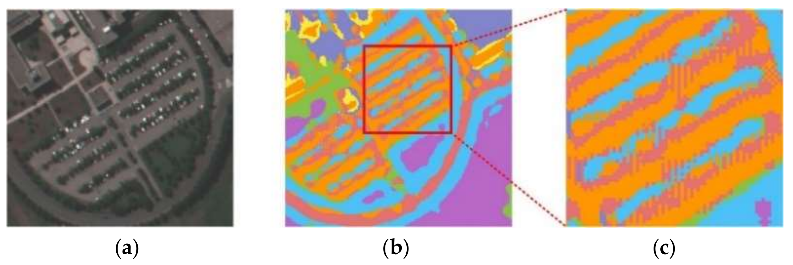
Remotesensing 11 02220 g001
Figure 2. The gridding problem resulting from dilated convolution. (a) True-color image of Pavia University. (b) Classification results with dilated convolution. (c) Enlarged classification results for (b).
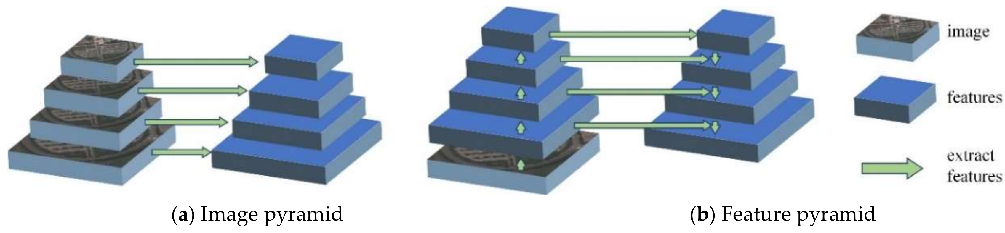
Remotesensing 11 02220 g002
Figure 3. The image and feature pyramid. (a) The image pyramid independently computes features for each image scale. (b) The feature pyramid creates features with strong semantics at all scales.
Remotesensing 11 02220 g003
Figure 4. An illustration of patch-based classification for hyperspectral image (HSI).
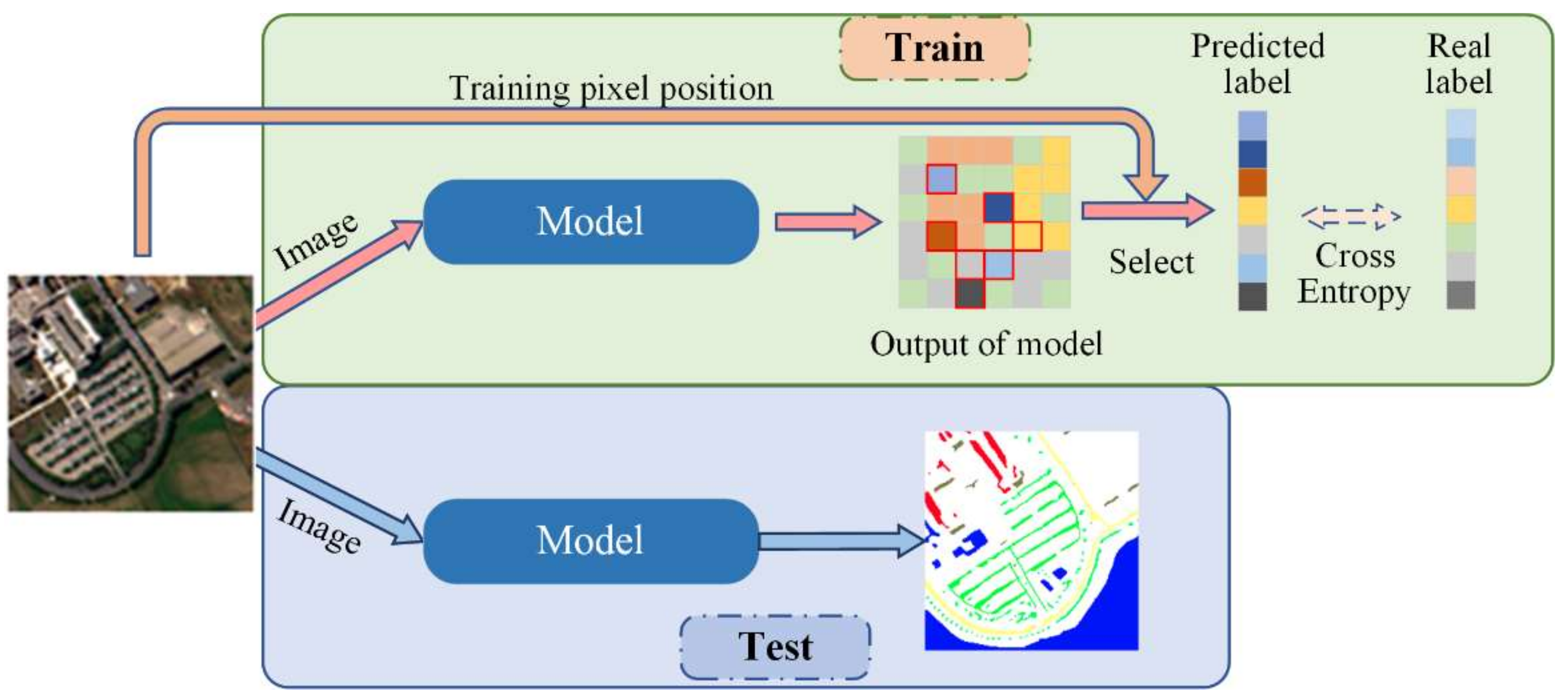
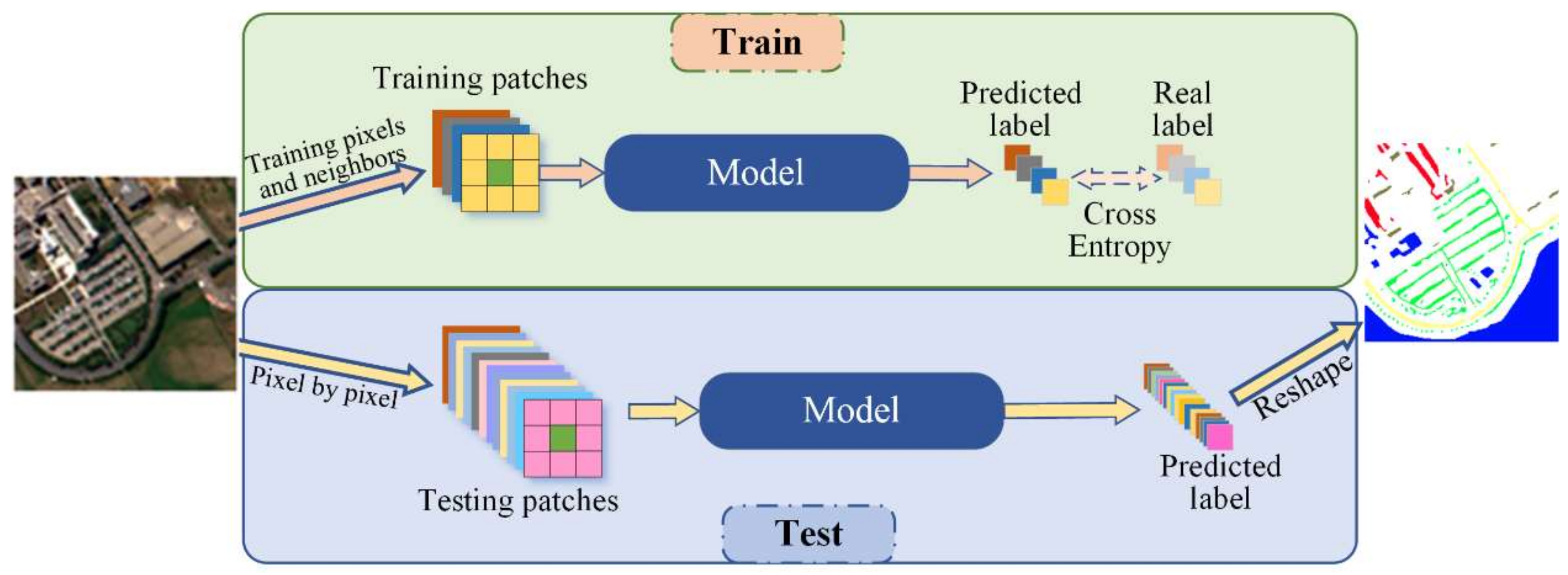
Remotesensing 11 02220 g004
Figure 5. An illustration of image-based classification for HSI. The model is similar to the segmentation model used in computer vision which takes an input of an arbitrary size and produces an output with a corresponding size. Additionally, the predicted labels should be selected in the output according to the training pixel position during training.
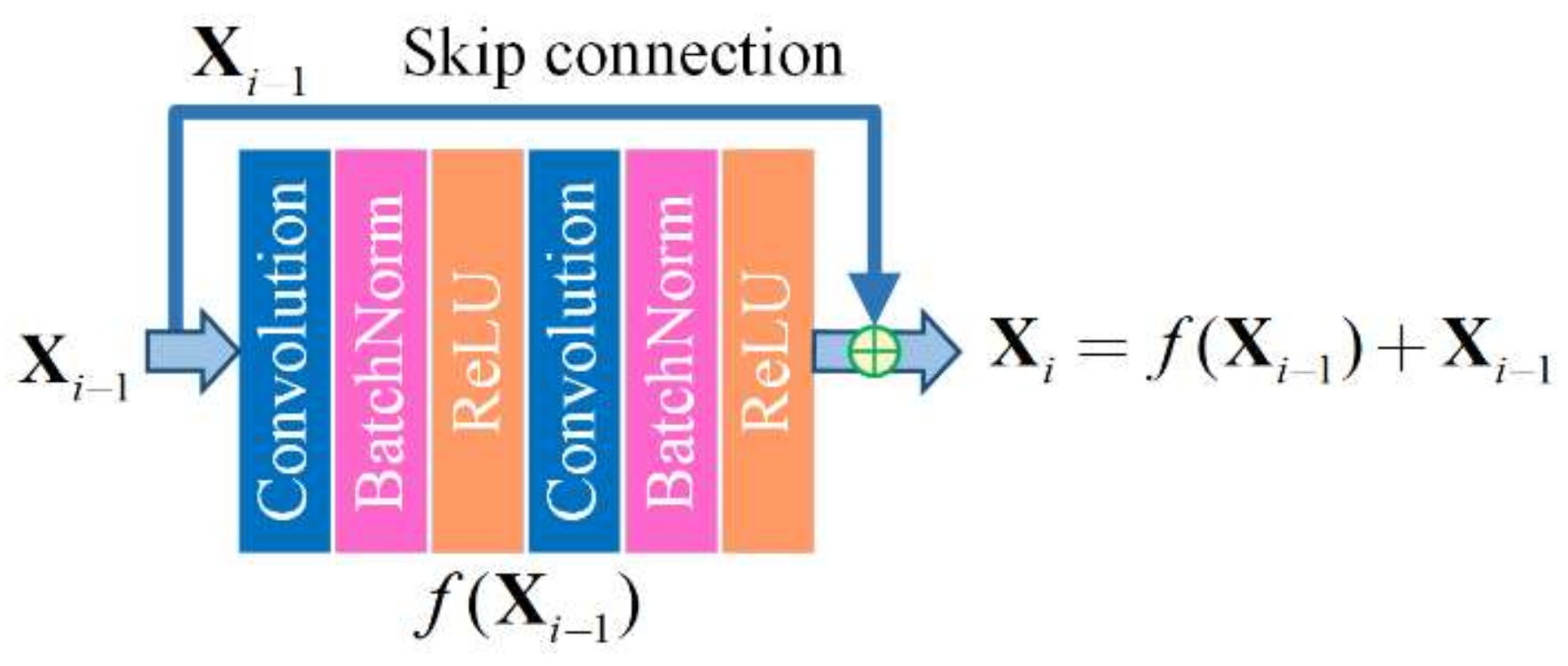
Remotesensing 11 02220 g005
Figure 6. An illustration of the residual block.
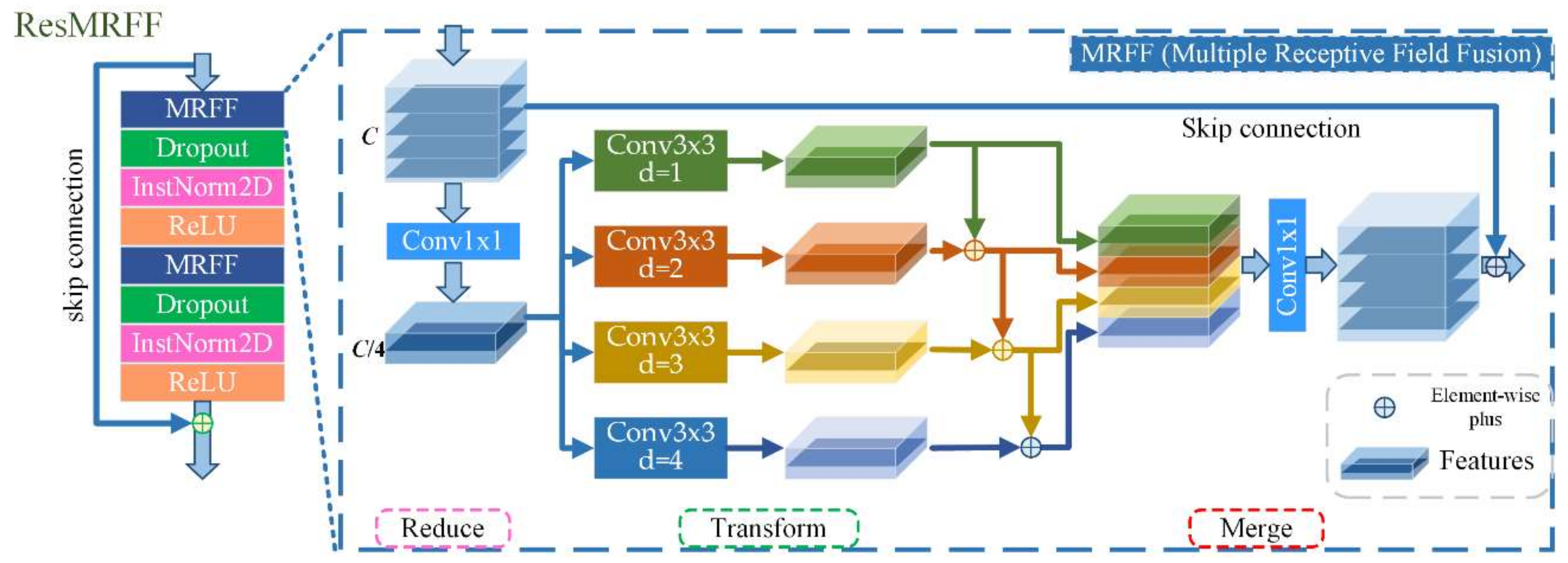
Remotesensing 11 02220 g006
Figure 7. A schematic of the residual multiple receptive field fusion block (ResMRFF). The basic strategy of the multiple receptive field fusion block is represented as Reduce-Transform-Merge.
Remotesensing 11 02220 g007
Figure 8. An illustration of the receptive field for the merged features in one MRFF block.
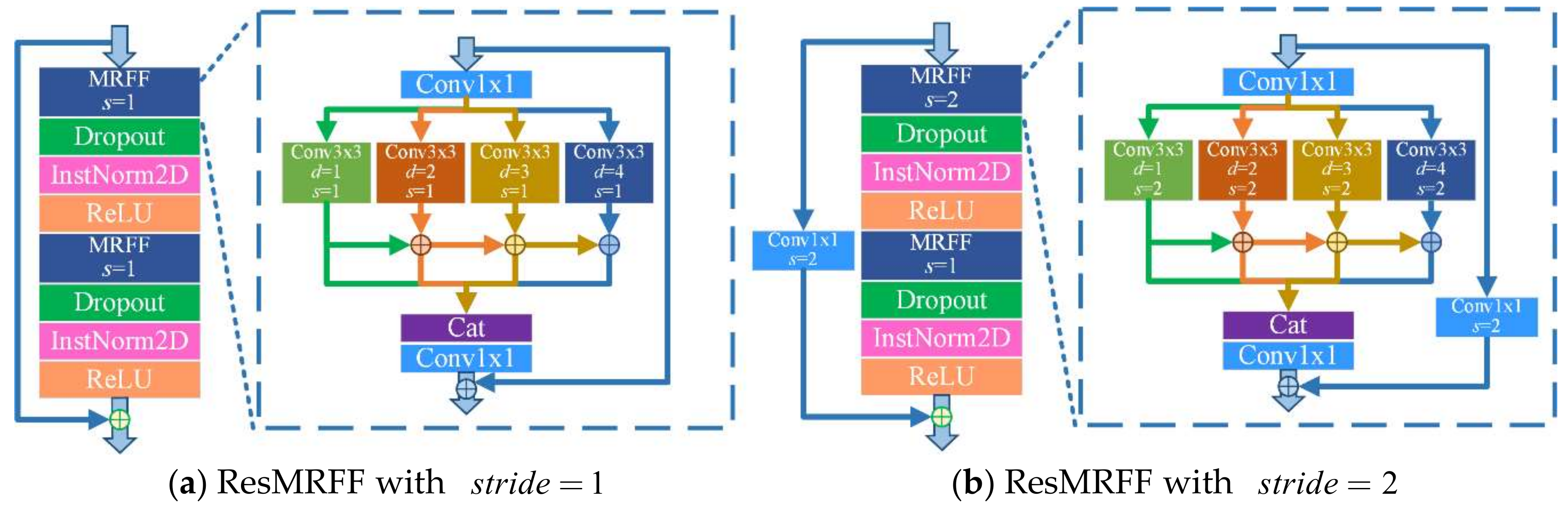
Remotesensing 11 02220 g008
Figure 9. An illustration of two ResMRFF blocks with different strides, where s refers to the convolution stride and d refers to the dilation factor. (a) refers to the ResMRFF block designed with stride=1, (b) refers to the ResMRFF block designed with stride=2.
Remotesensing 11 02220 g009
Figure 10. 
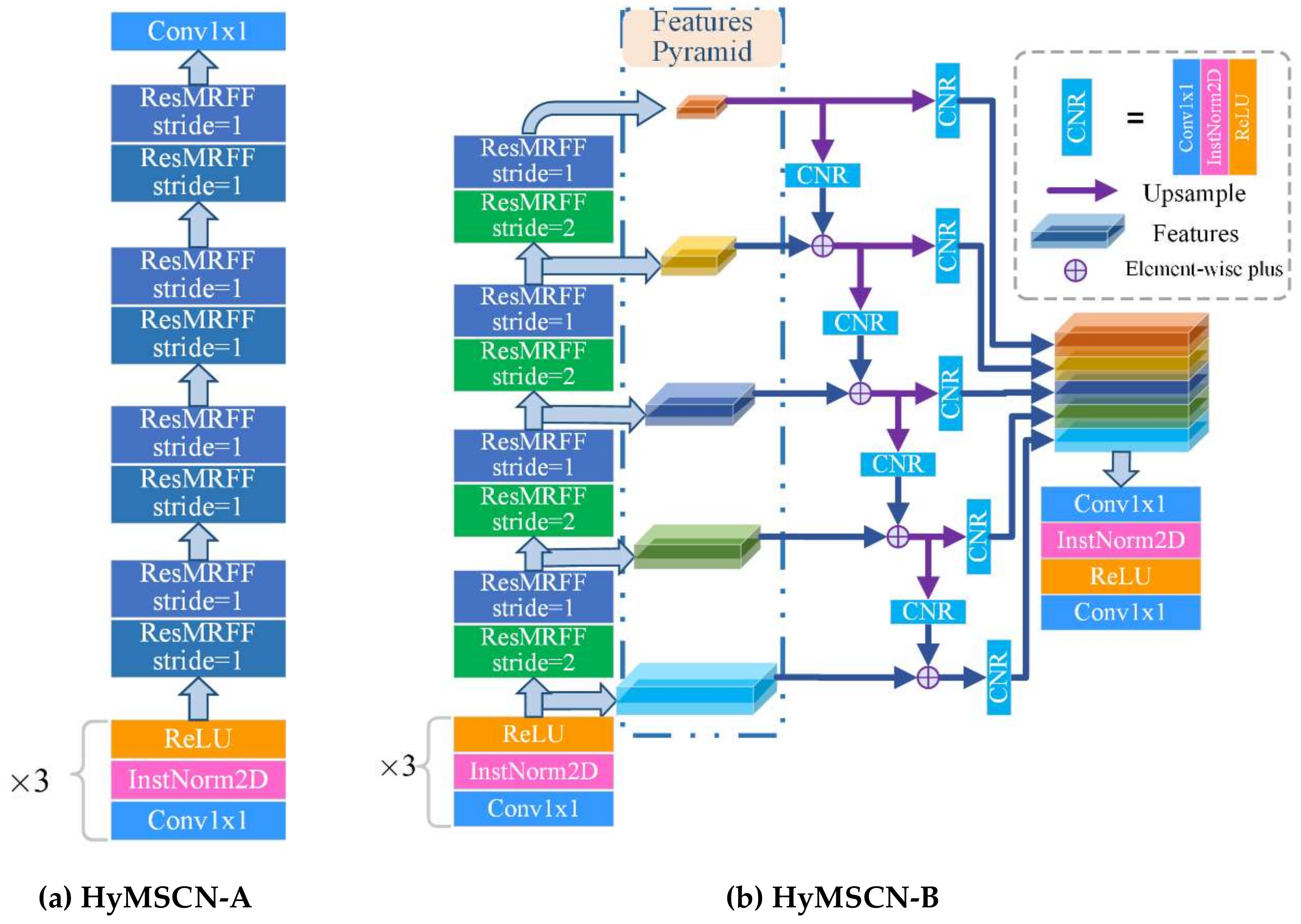
An illustration of the proposed two networks, (a) HyMSCN-A and (b) HyMSCN-B.
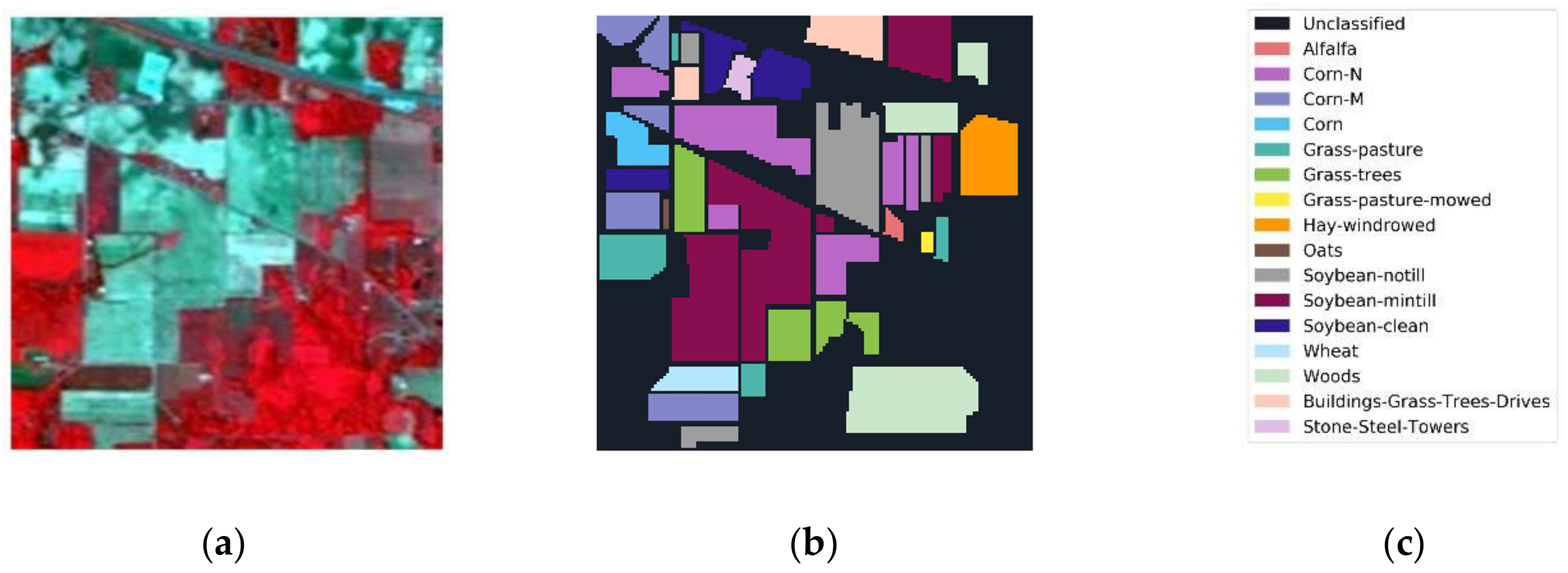
Remotesensing 11 02220 g010
Figure 11. Indian Pines imagery with (a) color composite, (b) reference data, and (c) class names.
Remotesensing 11 02220 g011
Figure 12. 
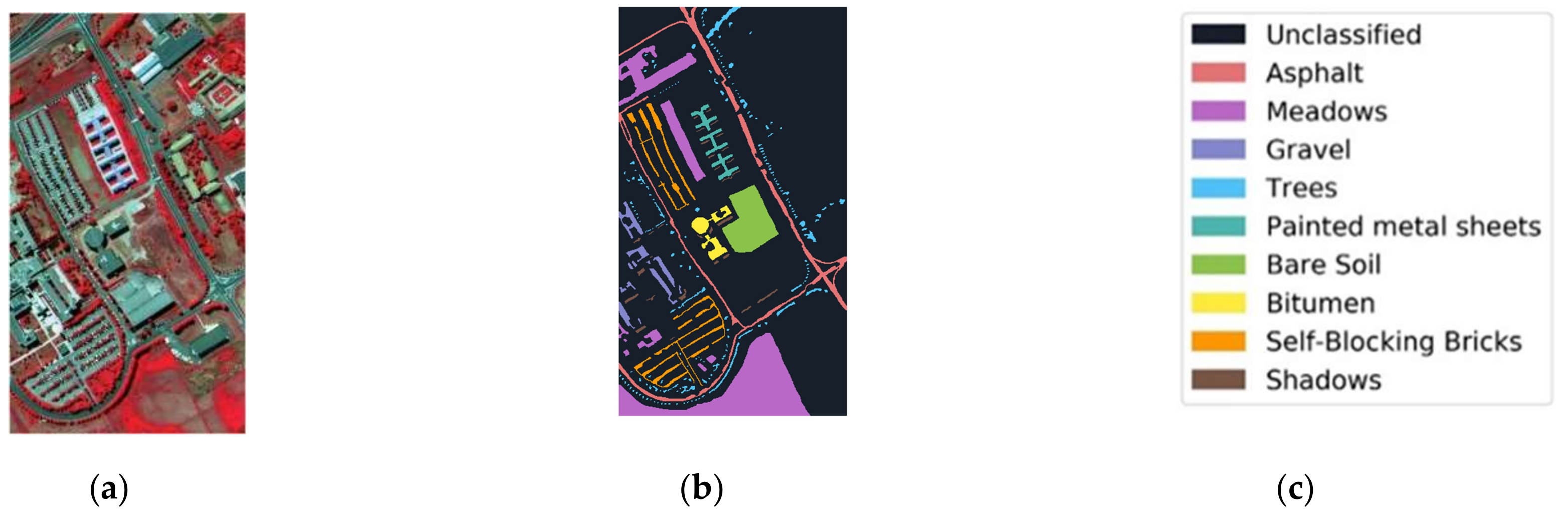
Pavia University data: (a) color composite, (b) reference data, and (c) class names.
Remotesensing 11 02220 g012
Figure 13. 
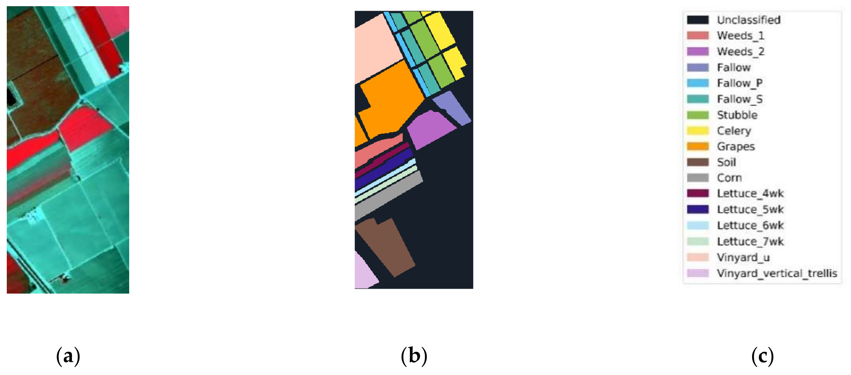
Salinas data: (a) color composite, (b) reference data, and (c) class names.
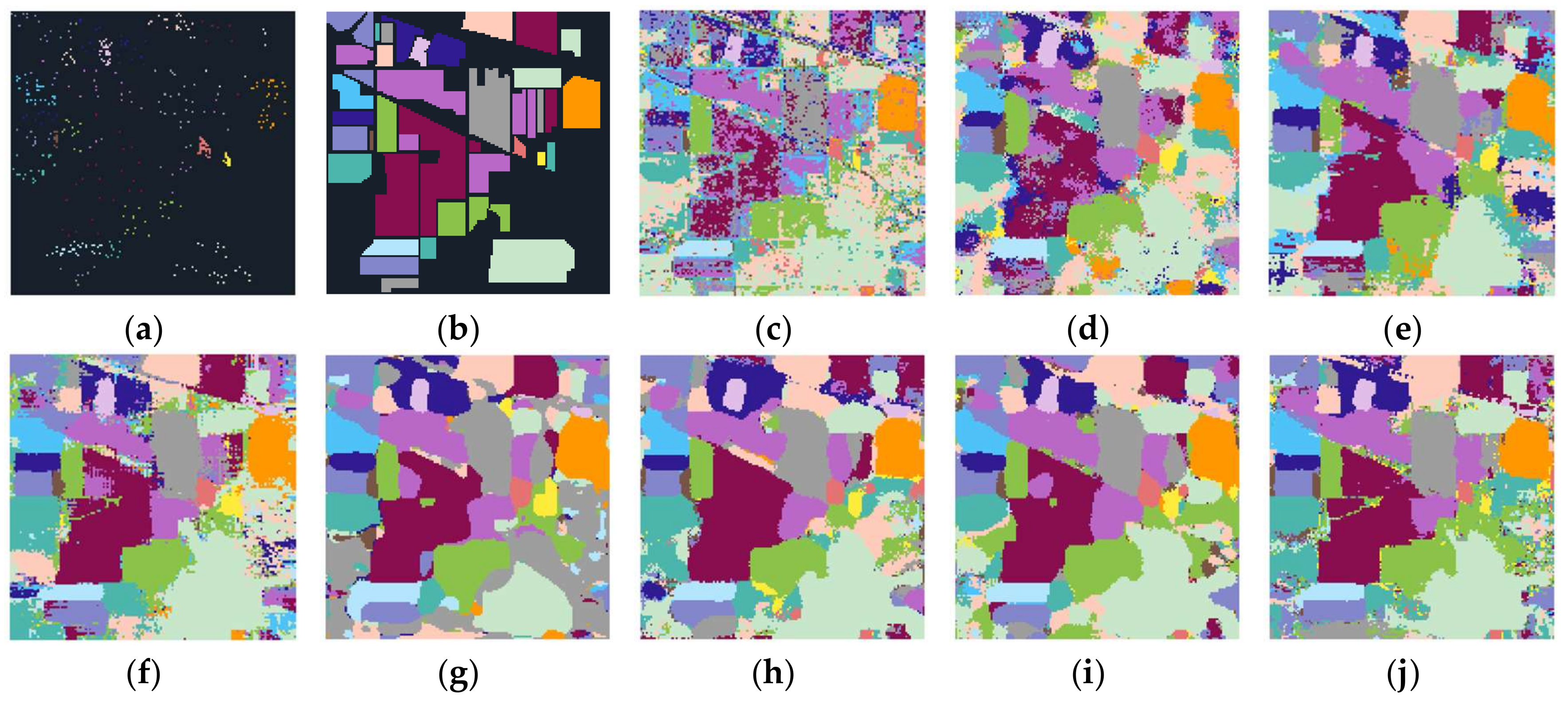
Remotesensing 11 02220 g013
Figure 14. Classification maps for Indian Pines data with 30 samples per class: (a) training samples, (b) ground truth, and classification maps produced by different methods, including (c) SVM (67.46%), (d) SSRN (78.66%), (e) 3DCNN (86.16%), (f) DCCNN (89.73%), (g) UNet (89.50%), (h) ESPNet (91.80%), (i) HyMSCN-A-128 (92.68%), and (j) HyMSCN-B-128 (93.73%).
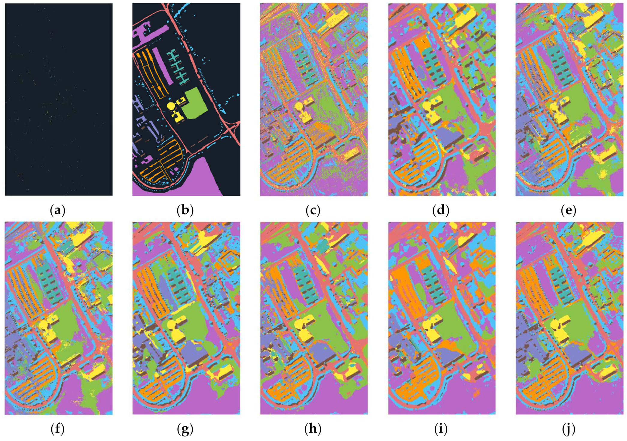
Remotesensing 11 02220 g014
Figure 15. Classification map for Pavia University data with 30 samples per class: (a) training samples, (b) ground truth, and classification maps produced by different methods, including (c) SVM (81.40%), (d) SSRN (81.51%), (e) 3DCNN (72.79%), (f) DCCNN (82.19%), (g) UNet (90.64%), (h) ESPNet (91.71%), (i) HyMSCN-A-128 (92.86%), and (j) HyMSCN-B-128 (96.45%).
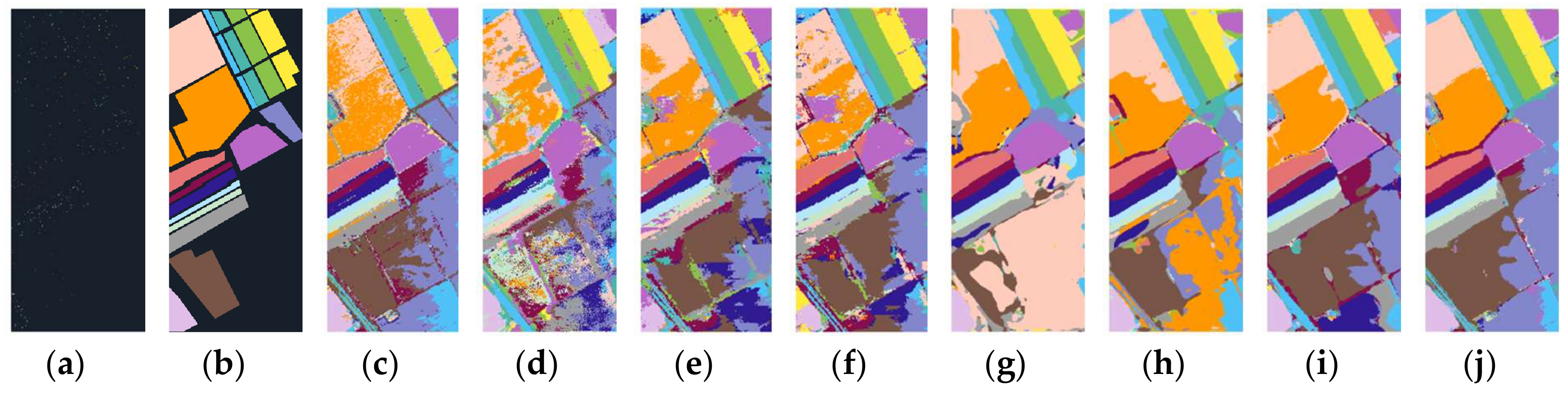
Remotesensing 11 02220 g015
Figure 16. Classification maps for Salina data with 30 samples per class: (a) training samples, (b) ground truth, and classification maps produced by different methods, including (c) SVM (88.48%), (d) SSRN (68.55%), (e) 3DCNN (80.99%), (f) DCCNN (82.42%), (g) UNet (84.38%), (h) ESPNet (87.85%), (i) HyMSCN-A-128 (97.05%), and (j) HyMSCN-B-128 (97.31%).
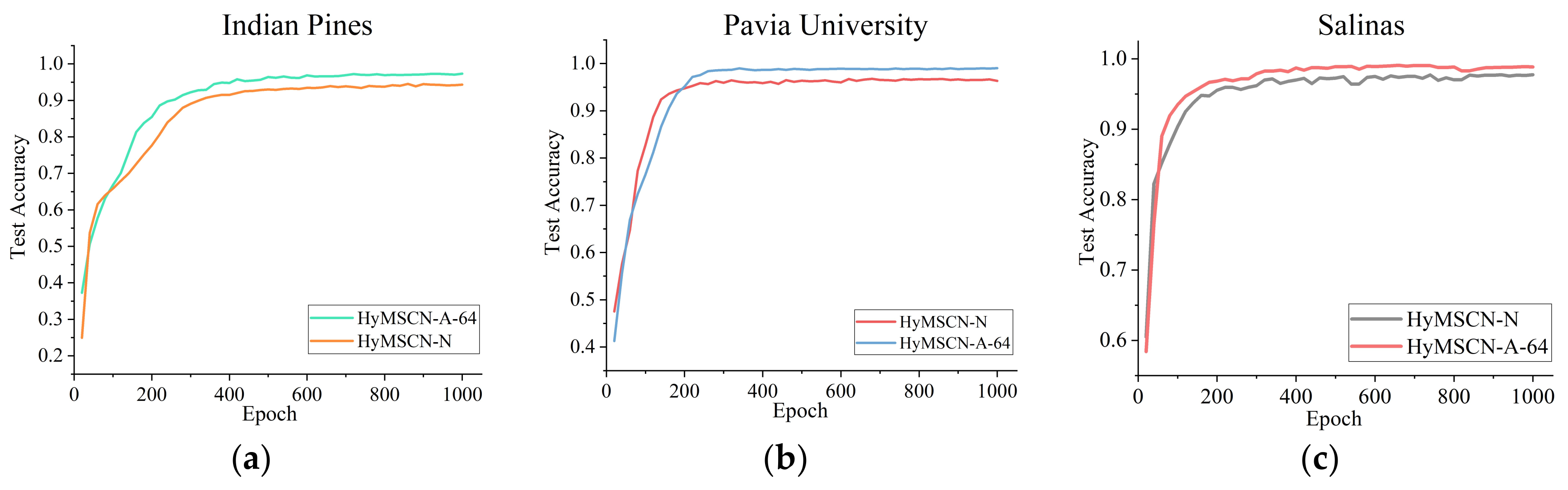
Remotesensing 11 02220 g016
Figure 17. An evaluation of the overall accuracy for multiple receptive field fusion (MRFF): (a) Indian Pines, (b) Pavia University, and (c) Salinas.
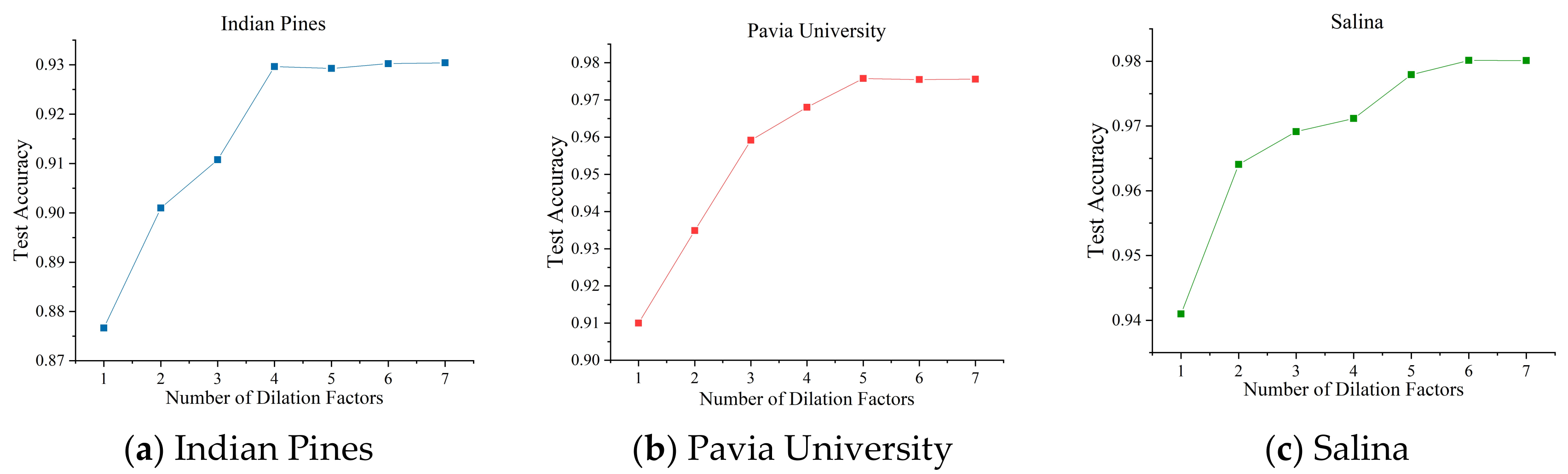
Remotesensing 11 02220 g017
Figure 18. Test accuracy for the different number of dilation factors in MRFF block. (a) Indian Pines data, (b) Pavia University data, (c) Salina data
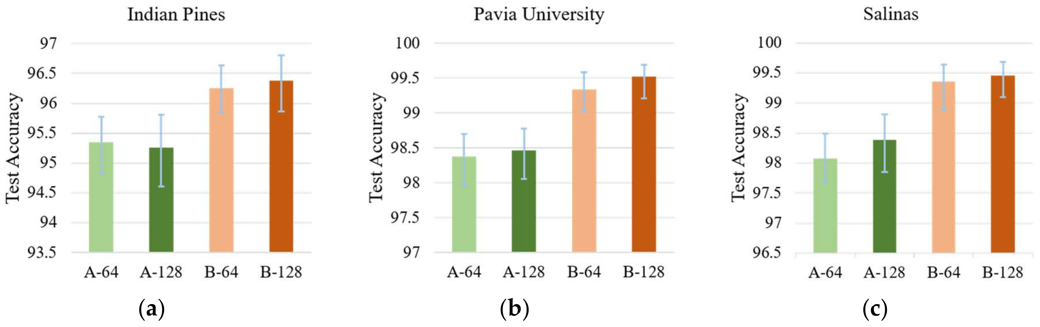
Remotesensing 11 02220 g018
Figure 19. The overall accuracy for different networks (A-64, A-128, B-64, and B-128 refer to HyMSCN-A-64, HyMSCN-A-128, HyMSCN-B-64, and HyMSCN-B-128, respectively). (a) Indian Pines, (b) Pavia University, and (c) Salinas.
Remotesensing 11 02220 g019
Table 1. The parameter settings of the proposed networks. The same colors refer to the same pyramid levels.
LayerHyMSCN-AHyMSCN-B
Output1StrideA-64 FeatureA-128 FeatureOutput1StrideB-64 FeatureB-128 Feature
CNR2 × 3145 × 14516464145 × 4516464
ResMRFF145 × 1451646473 × 7326464
ResMRFF145 × 1451646473 × 7316464
ResMRFF145 × 1451646437 × 3726464
ResMRFF145 × 1451646437 × 3716464
ResMRFF145 × 14516412819 × 19264128
ResMRFF145 × 14516412819 × 19164128
ResMRFF145 × 14516412810 × 10264128
ResMRFF145 × 14516412810 × 10164128
CNR----10 × 1016464
CNR----19 × 1916464
CNR----37 × 3716464
CNR----73 × 7316464
CNR----145 × 14516464
Note: 1 We used the spatial size of Indian Pines (145 × 145) as an example. 2 CNR refers to the convolution layer, normalization layer and ReLU activation function layer.
Table 2. Overall, average, k statistic, and individual class accuracies for the Indian Pines data with 30 training samples per class. The highest accuracies are highlighted in bold.
ClassTrain
(Test)
SVMSSRN3DCNNDCCNNUNetESPNetHyMSC-A1HyMSCN-B1
Alfalfa30(46)40.17%75.41%92.00%83.64%95.83%97.87%88.46%92.00%
Corn-no till30(1428)60.45%68.50%82.28%90.08%83.68%95.65%91.10%90.85%
Corn-min till30(830)54.72%75.95%72.50%77.05%88.11%86.10%86.37%84.57%
Corn30(237)31.33%67.16%77.63%85.25%86.05%89.39%86.76%94.42%
Grass-pasture30(483)78.95%77.45%91.07%91.52%94.22%99.52%94.29%95.01%
Grass-trees30(730)90.45%81.98%97.10%93.02%96.92%98.04%94.31%96.93%
Grass-pasture-m14(28)76.67%96.55%37.84%30.43%40.00%47.46%29.47%62.22%
Hay-windrowed30(478)99.53%92.02%97.54%97.15%100.00%95.98%99.38%99.17%
Oats10(20)45.45%48.78%80.00%64.52%80.00%90.91%71.43%86.96%
Soybean-no till30(972)51.41%68.28%73.24%79.98%73.24%80.21%81.48%88.14%
Soybean-min till30(2455)78.39%88.54%90.08%93.58%93.88%88.24%97.37%97.06%
Soybean-clean30(593)62.85%64.63%94.89%91.48%88.80%100.00%97.44%86.82%
Wheat30(205)92.61%89.04%97.10%93.58%90.71%99.03%99.51%99.03%
Woods30(1265)92.20%94.34%95.57%97.72%99.39%98.96%98.13%99.68%
Buildings/Grass30(386)41.78%75.08%76.56%98.21%88.40%93.90%98.44%97.72%
Stone-Steel-Towers30(93)98.89%68.38%92.00%76.03%93.94%89.42%96.84%97.89%
Overall accuracy67.46%78.66%86.16%89.73%89.50%91.80%92.68%93.73%
Average accuracy68.49%77.01%84.21%83.95%87.07%90.67%88.17%91.78%
k statistic0.63620.75960.84290.88330.8810.90650.91710.9287
1. HyMSCN-A and HyMSCN-B refer to the HyMSCN-A-128 and HyMSCN-B-128 networks, respectively.
Table 3. The overall accuracies obtained from various classification methods for Indian Pines data using different training samples. The best performances for each group are highlighted in bold.
SampleClassification Method
(Per Class)SVMSSRN3DCNNDCCNNUNetESPNetHyMSCN-A-128HyMSCN-B-128
160(10)58.42%68.79%67.58%71.84%74.03%78.95%76.22%82.29%
320(20)63.13%73.57%79.32%86.76%85.89%86.82%87.03%87.07%
444(30)67.46%78.66%86.16%89.73%89.50%91.80%92.68%93.73%
584(40)71.95%85.35%88.79%91.53%91.69%94.40%94.13%94.59%
697(50)72.54%89.26%90.49%94.06%94.83%95.78%95.26%96.37%
Table 4. Overall, average, k statistic, and individual class accuracy for Pavia University data with 30 training samples per class. The highest accuracies are highlighted in bold.
ClassTrain (Test)SVMSSRN3DCNNDCCNNUNetESPNetHyMSCN-A1HyMSCN-B1
Asphalt30(6631)93.78%89.53%98.77%98.45%94.25%98.64%99.44%99.55%
Meadows30(18649)91.07%98.54%99.66%99.36%99.85%99.51%99.99%99.67%
Gravel30(2099)71.87%56.11%39.76%57.16%56.08%68.90%89.53%95.41%
Trees30(3064)81.36%87.17%76.80%75.25%95.50%93.22%88.55%95.86%
Painted metal sheets30(1345)97.38%71.01%97.39%92.00%97.96%97.25%98.75%99.78%
Bare Soil30(5029)57.18%70.53%44.09%55.26%78.26%79.04%70.29%92.82%
Bitumen30(1330)47.34%59.75%73.55%82.47%73.20%71.70%95.82%99.70%
Self-Blocking Bricks30(3682)81.47%71.76%78.24%87.67%97.95%86.22%95.17%81.71%
Shadows30(947)99.89%77.71%97.83%98.85%93.20%96.53%100.00%99.68%
Overall accuracy (OA)81.40%81.51%72.79%82.19%90.64%91.71%92.86%96.45%
Average accuracy (AA)80.15%75.79%78.45%82.94%87.36%87.89%93.06%96.02%
k statistic0.75900.77160.6722 0.7792 0.87980.8920.90780.9535
1 HyMSCN-A and HyMSCN-B refer to the HyMSCN-A-128 and HyMSCN-B-128 networks, respectively.
Table 5. The overall accuracies produced by various classification methods for Pavia University data using a different number of training samples. The best performances for each group are highlighted in bold.
SampleClassification Method
(Per Class)SVMSSRN3DCNNDCCNNUNetESPNetHyMSCN-A-128HyMSCN-B-128
90(10)72.78%75.00%67.32%69.39%79.03%81.28%82.33%84.65%
180(20)78.33%79.81%68.91%74.62%80.75%87.11%88.90%95.80%
270(30)81.40%81.51%72.79%82.19%90.64%91.71%92.86%96.45%
360(40)83.28%85.87%80.07%83.45%91.52%95.14%96.54%98.23%
450(50)85.64%91.73%86.57%90.44%96.36%96.77%98.46%99.50%
Table 6. The overall, average, k statistic, and individual class accuracies for the Salina dataset with 30 training samples per class. The best results are highlighted in bold typeface.
ClassTrain (Test)SVMSSRN3DCNNDCCNNUNetESPNetHyMSCN-A-128HyMSCN-B-128
Weeds_130(2009)100.0%96.08%81.75%86.04%100.00%99.95%100.00%100.00%
Weeds_230(3726)98.31%84.44%63.46%66.73%99.76%100.00%100.00%99.97%
Fallow30(1976)96.84%87.23%69.81%78.31%88.68%98.91%99.31%99.90%
Fallow_P30(1394)94.62%93.80%96.08%96.66%48.96%61.11%90.23%96.07%
Fallow_S30(2678)98.82%83.29%85.24%93.72%77.14%72.03%99.69%99.47%
Stubble30(3959)99.92%84.01%90.32%94.94%99.22%99.42%100.00%99.92%
Celery30(3579)97.86%90.24%95.48%84.94%96.94%99.62%99.69%99.11%
Grapes30(11271)77.29%74.69%85.05%88.18%87.45%87.53%99.29%98.64%
Soil30(6203)98.79%96.89%81.87%95.62%94.74%99.73%99.92%99.53%
Corn30(3278)85.24%51.88%76.55%78.78%88.78%94.01%92.74%88.40%
Lettuce_4wk30(1068)79.75%28.17%62.67%63.40%93.97%91.98%87.41%86.40%
Lettuce_5wk30(1927)95.71%95.09%91.82%78.29%66.33%69.13%99.64%99.84%
Lettuce_6wk30(916)95.75%44.04%59.17%49.56%95.31%81.21%99.46%93.27%
Lettuce_7wk30(1070)83.80%19.30%77.90%77.25%98.97%89.70%98.70%97.03%
Vinyard_u30(7268)68.96%62.33%77.70%76.61%63.16%75.37%88.83%93.62%
Vinyard_vertical30(1807)99.35%64.61%97.36%93.81%100.00%92.32%99.94%99.94%
Overall accuracy88.48%68.55%80.99%82.42%84.38%87.85%97.05%97.31%
Average accuracy91.94%72.26%80.76%81.43%87.46%88.25%97.18%97.31%
k statistic0.87180.65660.7892 0.8065 0.82610.86490.96720.9701
Table 7. The overall accuracies produced by different classification methods for the Salina dataset using a different number of training samples. The best results are highlighted in bold type.
SampleClassification Method
(Per Class)SVMSSRN3DCNNDCCNNUNetESPNetHyMSCN-A-128HyMSCN-B-128
160(10)83.14%62.64%76.34%78.99%74.58%76.01%94.71%94.49%
320(20)87.11%66.16%79.05%80.12%83.63%85.15%94.82%96.51%
480(30)88.48%68.55%80.99%82.42%84.38%87.85%97.05%97.31%
640(40)90.71%77.80%86.50%87.37%91.84%93.03%98.15%99.38%
800(50)91.23%86.05%87.41%89.96%92.79%95.48%98.38%99.45%
Table 8. The training and testing times for patch-based and image-based classification. Each control group is highlighted with the same color.
Indian PinesPavia UniversitySalinas
SSRNSSRNHyMSCNSSRNSSRNHyMSCNSSRNSSRNHyMSCN
Patch Size79-79-79-
Train Maximum Batch Size510420145045016204601
Train Time of One Epoch (s)2.763.130.341.351.360.623.123.280.56
Test Maximum Batch Size6805301215015801215016201
Test Time of One Epoch (s)25.6535.400.11109.43339.670.4264.18115.690.41

