Article

Time Series GIS Map Dataset of Demolished Buildings in Mashiki Town after the 2016 Kumamoto, Japan Earthquake

by
Yuzuru Kushiyama
1,* and
Masashi Matsuoka
2
1
Department of Built Environment, Tokyo Institute of Technology 4259-G3-2 Nagatsuta, Midori-ku, Yokohama 226-8502, Japan
2
Department of Architecture and Building Engineering, Tokyo Institute of Technology 4259-G3-2 Nagatsuta, Midori-ku, Yokohama 226-8502, Japan
*
Author to whom correspondence should be addressed.
Remote Sens. 2019, 11(19), 2190; https://doi.org/10.3390/rs11192190
Submission received: 10 August 2019 / Revised: 2 September 2019 / Accepted: 13 September 2019 / Published: 20 September 2019

Abstract

:
After a large-scale disaster, many damaged buildings are demolished and treated as disaster waste. Though the weight of disaster waste was estimated two months after the 2016 earthquake in Kumamoto, Japan, the estimated weight was significantly different from the result when the disaster waste disposal was completed in March 2018. The amount of disaster waste generated is able to be estimated by an equation by multiplying the total number of severely damaged and partially damaged buildings by the coefficient of generated weight per building. We suppose that the amount of disaster waste would be affected by the conditions of demolished buildings, namely, the areas and typologies of building structures, but this has not yet been clarified. Therefore, in this study, we aimed to use geographic information system (GIS) map data to create a time series GIS map dataset with labels of demolished and remaining buildings in Mashiki town for the two-year period prior to the completion of the disaster waste disposal. We used OpenStreetMap (OSM) data as the base data and time series SPOT images observed in the two years following the Kumamoto earthquake to label all demolished and remaining buildings in the GIS map dataset. To effectively label the approximately 16,000 buildings in Mashiki town, we calculated an indicator that shows the possibility of the buildings to be classified as the remaining and demolished buildings from a change of brightness in SPOT images. We classified 5701 demolished buildings from 16,106 buildings, as of March 2018, by visual interpretation of the SPOT and Pleiades images with reference to this indicator. We verified that the number of demolished buildings was almost the same as the number reported by Mashiki municipality. Moreover, we assessed the accuracy of our proposed method: The F-measure was higher than 0.9 using the training dataset, which was verified by a field survey and visual interpretation, and included the labels of the 55 demolished and 55 remaining buildings. We also assessed the accuracy of the proposed method by applying it to all the labels in the OSM dataset, but the F-measure was 0.579. If we applied test data including balanced labels of the other 100 demolished and 100 remaining buildings, which were other than the training data, the F-measure was 0.790 calculated from the SPOT image of 25 March 2018. Our proposed method performed better for the balanced classification but not for imbalanced classification. We studied the examples of image characteristics of correct and incorrect estimation by thresholding the indicator.

Graphical Abstract

1. Introduction

1.1. Background

After a large-scale disaster, damaged buildings are demolished not only to prevent the occurrence of secondary damage but also to rebuild the living environment. As many damaged buildings are demolished, a large amount of disaster waste is generated. If the disposal of disaster waste is slow, it can cause problems, such as a delay to recovery and reconstruction, outflow of hazardous materials, and outbreaks of epidemic and infectious diseases in the affected area. It is thus necessary to properly and smoothly dispose the disaster waste. For an appropriate implementation plan of disaster waste disposal, it is required to estimate the amount of disaster waste generated in an early phase after the disaster. Estimation equations for the amount of generated disaster waste have been determined by a regression analysis of past disasters based on the total amount of disaster waste disposed and the total number of damaged buildings at the prefecture and city levels [1,2,3,4]. The conventional equation for estimating the amount of disaster waste generated is calculated by multiplying the number of severely and moderately damaged buildings, a coefficient value that represents the ratio of the number of demolished building to the number of severely and moderately damaged buildings, and the disaster waste disposal generation intensity per building.
In the 2016 Kumamoto disaster, two large earthquakes of M6.5 on 14 April and M7.3 on 16 April occurred near Mashiki town, causing major damage to many buildings (Figure 1). Kumamoto Prefecture reported that approximately 210,000 buildings in Kumamoto prefecture and 15,300 buildings in Mashiki town were damaged [5,6].
As Mashiki town was close to the epicenters, around 30% of the damaged buildings were severely damaged and many buildings needed to be demolished. Demolished buildings are generally treated as disaster waste disposal. At the completion of its disposal, Kumamoto Prefecture reported that the amount of disaster waste in Kumamoto prefecture was approximately 3 million tons [5] and that of Mashiki town was 337,629 tons [6]. In order to smoothly implement disaster waste disposal, it is necessary to estimate the amount of disaster waste disposal and draw up an implementation plan that includes schedules, securing of a temporary site, equipment, and team organization. The Kumamoto Prefectural government estimated that the amount of disaster waste disposal would be 1 to 1.3 million tons on 18 May 2016, prior to the completion of the survey of the damaged buildings. On 1 June 2016, the Kumamoto Prefectural government reported the number of majorly and moderately damaged buildings as 8641, and 34,352. The disaster waste was estimated again approximately 2 million tons, which was calculated by the conventional equation (1) as below;
( 8641 × 1.0 + 34 , 352 × 0.2 ) × 117 = 1 , 814,834   tons ,
where the value 1.0 and 0.23 is the ratio of the number of demolished buildings to the number of majorly and moderately damaged buildings, and the value, 117 (tons per building) is the disaster waste disposal generation intensity per building. Compared to the estimated value of June 2016, the final value of March 2018 was 1.6 times greater. The report of the Mashiki municipality [6] suggested that the actual number of the demolished buildings might be larger than the estimated number based on the damaged buildings because the disaster waste was possibly derived from buildings not registered in the Mashiki administration.
We consider that the total volume of disaster waste disposal depends on the actual number of demolished buildings, the floor area of buildings, and the typologies of building structures, such as wood or concrete construction. In past research, however, demolished buildings were not individually identified, and the percentage of damaged buildings that were demolished, the total floor area, and the proportions of structure typologies were not clarified. Therefore, it is necessary to create a dataset to identify demolished and remaining buildings.
In addition, we aimed to identify the demolished and remaining buildings, not only at the completion of the disaster waste disposal, but also as a time series in order to obtain a more accurate estimation of the relationship between disposal generation and demolished buildings, using the monthly amount of disaster waste disposal recorded in the Mashiki municipality. Therefore, we tried to identify all the demolished and remaining buildings in Mashiki town, and to create a time-series of a geographic information system (GIS) map dataset using satellite images observed from the early phase following the 2016 Kumamoto earthquake until disaster waste disposal was completed. As the town has been reconstructed as the recovery proceeds, the time series GIS distribution map data of demolished buildings are possibly used to monitor the status for demolishing as well as for reconstruction.

1.2. Review and Objectives

In order to create a GIS map dataset with labeling of demolished and remaining buildings, we researched prior investigations related to building extraction using satellite images and GIS map data including building footprints. We found existing studies related to building extraction and creation of building footprints that used very high resolution (VHR) optical satellite images, which have higher than one-meter resolution, such as IKONOS, QuickBird, WorldView, and Pleiades. To classify areas where buildings were damaged by an earthquake, Yamazaki and Matsuoka (2007) studied pixel-based and object-based land cover classifications using VHR optical satellite images and compared the result of classification with visual interpretation [7]. They suggest the possibility of extracting the extent of severely damaged buildings via object-based classification. Automatic building detection from VHR satellite images has become an increasingly important issue. For the purpose of building detection, a training dataset for deep learning has been created from high definition aerial photographs and VHR satellite images, and many studies have been conducted with them [8,9,10]. Many building detection methods using convolutional neural networks (CNN) have been studied, which require a training dataset of many labeled buildings and VHR images. The Inria aerial image dataset consists of labeled buildings and 180 color image tiles of size 5000 × 5000, covering an area of 1500 m × 1500 m at 30 cm resolution. In the Inria contest, solutions used U-Net or SegNet approaches for segmentation and extraction for buildings [11].
Recently, as the resolution of satellite images has improved to 30 cm, competitions that provide training datasets of VHR satellite image were held to compete for building detection accuracy. The SpaceNet [12] building dataset, which contains WorldView-2/3 multispectral band images covering some cities (e.g., Las Vegas, Paris, Shanghai, and Khartoum) and building footprints was provided. Several competitive methods using the dataset were explored in the DeepGlobe Satellite Challenge of the Institute of Electrical and Electronics Engineers (IEEE) Conference on Computer Vision and Pattern Recognition 2018 (CVPR 2018) [13]. Hamaguchi and Hikosaka (2018) developed a U-Net based semantic segmentation method that can analyze image fitting to buildings of different sizes through the competition and improved the model compared to the conventional U-Net model [14].
As the public GIS map data have been recorded, an approach combining GIS map data and satellite images for building extraction monitoring is also conceivable. Huang et al. (2018) created a high-quality Vancouver building dataset from DEIMOS-2, with 1-m pan-sharpened images whose ground-truth was obtained from GIS map data [15]. They used the dataset for a building extraction method via deep deconvolution neural networks. Yuan et al. (2014) presented a method for automatically counting buildings using a dataset of aerial images and building footprints of GIS maps [16]. They observed that the number of buildings in an image is linearly correlated to the line segment number derived from building counts. Du et al. (2015) combined VHR images with GIS map data in a random forest method with fine categories in order to improve the classification of urban buildings [17]. Li et al. (2019) combined VHR satellite images in the SpaceNet dataset with GIS map data from multiple sources of map data [18] (e.g., OpenStreetMap (OSM) [19], Google Maps [20], and MapWorld [21]) and explored the enhancement of the total F1-score compared with the methods in the previous SpaceNet Building Detection Competition. We found that semantic segmentation using GIS map data and VHR satellite images or high definition aerial photographs was useful for building extraction. However, it has not been verified whether this method can be adopted to satellite images of resolution lower than 1 m.
Many researchers have studied the issue of monitoring urban areas using high resolution (HR) satellite images, such as SPOT-1-5, and medium resolution (MR) satellite images, such as Landsat and Sentinel-2, whose data has been obtained widely and accumulated for several years [22,23,24]. As the purpose of these studies is to identify the extent of urban areas and to monitor their change via identification of building structures, roads, etc., such methods are inadequate to identify individual buildings through analysis of HR and MR satellite images.
As the purpose of this study was to create a time series GIS map dataset of buildings from the early phase following the 2016 Kumamoto earthquake until the completion of disaster waste disposal, we needed to obtain satellite images observed within a few months of the earthquake. With this aim, we searched WorldView-3 images with 30-cm resolution and found two scenes using search criteria of: Approximate area of 65 km2; boundaries of 10 km to the east and west of Mashiki town; less than 20 percent cloud; less than 20 degree incidence angle; and, within one year from 16 April 2016 to 15 April 2017. Similarly, one scene from 50-cm-resolution Pleiades satellite images was found for the same period and conditions, and we found seven scenes from SPOT-6 and 7 with 1.5-m resolution. If we aim to establish a time series of building changes one year after the Kumamoto earthquake using currently operating satellites, we should consider a proposed method to identify demolished and remaining buildings using HR rather than VHR satellite images. Therefore, we aimed to select appropriate GIS map data and HR satellite images, establish a method to identify demolished and remaining buildings, and create a time series GIS map dataset until the completion of disaster waste disposal following the 2016 Kumamoto earthquake.
Our two major objectives can be summarized as follows: (1) Create a time series GIS map dataset with labels of demolished and remaining buildings until disaster waste disposal was completed in Mashiki town, and (2) propose a method to identify demolished and remaining buildings, integrating GIS map data and time series HR satellite images, and verify the effect of this method.

2. Materials and Methods

We aimed to use GIS map data, including buildings existing in Mashiki town at the time of the earthquake, and HR satellite images, to label buildings as demolished or remaining during the two-year period following the earthquake. For this purpose, we selected the appropriate GIS map data describing the building footprint of Mashiki town at the time of the event and satellite data observed several times within the two-year period. Next, we created supporting information to help identify the demolished and remaining buildings using the selected satellite images and GIS map data including the building footprint. For creation and evaluation of the supporting information via image analysis, a training and test dataset was needed, for which demolished and remaining buildings should be confirmed through field surveys and image interpretation. The output was the time series GIS map dataset with labels of demolished and remaining buildings by visual interpretation with reference to the supporting information.

2.1. Preparation of Satellite Images and GIS Map Data

We selected HR satellite images that covered the whole Mashiki town with less than 10% cloud condition between March 2016 and March 2018. Since SPOT satellite images have been more frequently acquired than other VHR/HR satellite images, we tried to use SPOT images for image analysis and visual interpretation. To provide a base for comparison, we selected one scene of Mashiki town observed on 20 March 2016, one month before the earthquake occurrence. We then selected three post-disaster images: One from 29 July 2016, two months after the disaster waste disposal plan was announced; one from 1 January 2017, half a year after the first scene; and one from 25 March 2018, when disaster waste disposal for the whole of Mashiki town was almost completed. As an area of approximately 0.3 km2 in the image on 29 July 2016 was covered with cloud, we selected an image from 11 August 2016 (i.e., close to 29 July) in order to interpolate or complement the area covered with cloud. Although we could not find multiple Pleiades or WorldView images within one year of the earthquake, we confirmed the situation of demolished building via visual interpretation and chose two images intermediately after disaster waste disposal was finished. The selected observation date, satellite name, resolution, incidence angle, and usage are shown in Table 1. Second, we selected GIS map data, including the footprints of individual buildings in Mashiki town, near the time of the earthquake to understand the situation of existing buildings before the earthquake, and to label demolished and remaining buildings by analysis and visual interpretation of satellite images. The OSM data contained suitable building footprint information, because OSM was used in previous research for the improvement of building detection [18]. We found the OSM data that were representing the existing buildings in Mashiki town before the earthquake. They contained footprints that described the area and outline of the individual buildings. Thus, we decided to use the OSM data as a base map.

2.2. Strategic Approach in this Study

We needed to consider a methodology to efficiently create the time series GIS map dataset with labels for demolished and remaining buildings using OSM data and several scenes of satellite images, as shown in Table 1. Visual interpretation of every building of the OSM data through all images is one such method. However, there are approximately 15,300 buildings in Mashiki town, so it would take considerable time for visual interpretation, comparing the before and after SPOT and Pleiades images shown in Table 1, and labeling every building. In order to shorten the time for interpretation and labeling, we analyzed integrated GIS map data and images, and created supporting information that makes it easy to identify demolished buildings. As previously mentioned, a method based on CNN requires the preparation of many training datasets and it takes considerable time to create learning data. As we preferred to focus on the image analysis, we designed the following strategic approaches:
  • We minimized time to create training data.
  • We created supporting information via image analysis, and confirmed demolished and remaining buildings through visual interpretation referring to this information.
  • We distributed the supporting information on individual buildings.
  • The supporting information likely enhanced the understanding of differences in images of demolished and remaining building.
The process of the numbered boxes from (1) to (8) in Figure 2 is described in the following Section 2.2.1, Section 2.2.2, Section 2.2.3, Section 2.2.4, Section 2.2.5, Section 2.2.6, Section 2.2.7 and Section 2.2.8.

2.2.1. Download OSM Data and Refining by Attribute

We downloaded and extracted OSM data within the Mashiki town boundary. We found the OSM data had 17,190 polygons whose attributes were not only buildings but also other categories: Green houses, farms, and so on. We narrowed down the OSM data to the attributes related to buildings: Apartments, buildings, houses, and residential. As a result of narrowing down by attribute, the OSM data of Mashiki town was reduced to 15,794 polygons. The OSM data before and after refining are shown in Figure 3.
We considered whether the refined OSM data contained all building polygons in Mashiki Town. According to the 2013 Housing and Land Statistics Survey [25], the total number of residential houses in Mashiki town was 10,700. However, there are buildings other than houses in Mashiki town and, according to the records of the Mashiki municipality [7], the total number of buildings in Mashiki town was 15,304 at the time of the earthquake. The number of polygons in the OSM data refined by the attributes related to building was larger than the number of the municipality record. Moreover, we also checked if buildings were not recorded in the OSM data by referring the OSM building-related data to the satellite images of Mashiki town, finding 312 buildings that were not recorded in the OSM data (as shown in Figure 4).
The total number of buildings was 16,106, as we merged the buildings of the OSM data and the buildings found out of the OSM data. In this research, we decided to use the merged data of buildings, which is defined as Mashiki building map data. The Euler diagram of Figure 5 shows the relationship between all buildings (Mashiki building map data), the OSM data of buildings, demolished buildings, and buildings in the registry book of the Mashiki administration.

2.2.2. Geometric Correction and Orthorectification

We overlaid the OSM data on the satellite images listed in Table 1 and found a geolocation gap caused by topography and satellite position. We orthorectified the satellite images using the software ENVI, rational polynomial coefficients (RPC) files attached to the satellite images, and the 10-m digital terrain model (DTM) of the Geospatial Information Authority of Japan [26] for topographic data. We measured the coordinate at a corner of a building nearby a road by a GPS receiver. We compared the position of the building corner in the satellite images with the position that is measured by GPS as latitude 32.78669444, longitude 130.80778611. The geolocation gaps between the measured position (green X ) and the position of the building corner (red +) in the satellite images were within 3 m, i.e., two pixels of the SPOT image (Figure 6).
We also found the clearly ridged building, which is drawn in the blue outlined footprints of the OSM data and compared the footprint with the position of the building in the satellite images. The geolocation gaps between the footprint and the building position in the satellite images were negligible.

2.2.3. Field Survey Around the Demolished Building

In order to efficiently identify demolished and remaining buildings, we investigated and compared the characteristics of the demolished and remaining buildings on the images, and created a dataset with satellite images and sample labels of demolished and remaining buildings via a field survey. We researched the demolished buildings on site, where we found and visually inspected many demolished buildings in the satellite image. We classified many demolished buildings as remaining buildings in the area. Figure 7 shows some examples of photos taken during the site survey. The locations where these photos were taken are plotted on the satellite image shown in Figure 8.

2.2.4. Labeling for Demolished/Remaining Buildings by Field Survey and Visual Interpretation

The SPOT images shown in Table 1 were observed on 20 March 2016, 29 July 2016, 1 January 2017, and 25 March 2018, and we selected samples of buildings that were labeled as demolished, including on the three observation dates after the earthquake, to determine the characteristics of the images around the buildings. Based on visual interpretation of the post-earthquake SPOT images and the field survey, we attached 55 demolished and 55 remaining labels to the Mashiki building map data of buildings for a training dataset as shown in Table 2.

2.2.5. Calculation for Characteristics of Satellite Images

It is well known that brightness and intensity balance among bands of images differ due to the season and that land surface features change due to vegetation. We measured the distribution of each image on the three acquisition dates, before and after demolition of buildings, before we looked at the image characteristics. In order to avoid the effect of vegetation change, we extracted the image characteristics within the footprint of the Mashiki building map dataset of the buildings. Figure 9 shows the histogram distribution and average values of the digital number (DN) in the footprints of SPOT images on each date.
Based on Figure 9a,b, we found the average DN of the images observed on 29 July 2016 was higher than the average DN of the images on 20 March 2016 before the disaster. From Figure 9a,c, the average DN of images on 1 January 2017 was lower than the average DN of the images on 20 March 2016, and the average DN definitely changed depending on the season. Although the observation month is the same, there is a difference between the average DN on 20 March 2016 and on 25 March 2018, as shown in Figure 9d. We were thus able to adjust the different average DN among the images.

2.2.6. Establishment of the Model by the Indicator

We used the Mashiki building map dataset with labels of demolished and remaining buildings as shown in Table 2 to investigate the features of the satellite images around the buildings. We overlaid the Mashiki building map dataset labels on the SPOT satellite images observed on 20 March 2016, 29 July 2016, 1 January 2017, and 25 March 2018, as listed in Table 1. Figure 10 shows the demolished buildings, remaining buildings, and others labeled in the Mashiki building map dataset. SPOT and Pleiades satellite images shown in Table 1 have multispectral band data and it is possible to create pan-sharpened images. However, we decided to use mainly panchromatic images due to their contrast, brightness, and sharpness, which make it easier to confirm the changes. We compared the area around the demolished and remaining buildings and found that the image pixels of the area around demolished buildings became brighter. To make the best use of this change in brightness, we considered that the brightness of the entire image changes depending on the observation date as described in Section 2.2.4. If we simply calculated the difference, some changes of demolished buildings might be lost. Thus, we needed to consider an image analysis method based on the brightness change of the area around the demolished building that accounted for the change due to the observation date. Accordingly, we used binary data, which was set to 1 if the image pixel was larger than the average DN shown in Figure 9, and 0 if it was smaller than the average DN, as follows:
A v e r a g e = i = 1 N D N i N ,
where N is number of pixels within a building polygon in the whole image.
B i n a r y = { 1 ,   ( D N > A v e r a g e ) 0 ,   ( D N A v e r a g e ) .
We created a binary image from the satellite images of each observation date via Equations (2) and (3). Figure 11a–d shows the binary images for the same frames as shown in Figure 10a–d, respectively.
We found that binary data values of 0 in Figure 11a changed to 1 in the polygon of the demolished building in Figure 11b–d, and it seemed that a higher proportion of the binary data changed in the polygons of demolished buildings than of the remaining buildings. By setting binary data created from the image before the earthquake as binary before, and binary data created from images after the earthquake as binary after, we could determine a binary flag that indicated a change of binary data. Then we calculated the ratio of the binary flag to pixels within the building polygon as:
B i n a r y _ f l a g = { 1 ,   ( B i n a r y _ a f t e r B i n a r y _ b e f o r e > 0 ) 0 ,   ( otherwise ) ,
R a t i o = i = 1 M B i n a r y _ f l a g i M ,
where M is the number of pixels within a polygon.
We calculated the ratio for all buildings based on Equations (4) and (5). The ratio indicated the possibility of a demolished building if the ratio was large and a remaining building if it was small. We applied the indicator to the images of 29 July 2016, 1 January 2017, and 25 March 2018, forming a relationship of the indicator to the Mashiki building map dataset, and created the indicator distribution map as shown in Figure 12.

2.2.7. Evaluation of the Indicator

The performance of the indicator is able to be evaluated by the receiver operating characteristics (ROC) curve [27], which is an effective tool for the evaluation of classification. In order to draw the ROC curve, we described the estimation result by the indicator and the actual building situated in the confusion matrix as Table 3. We defined the estimation result as positive if the building was estimated as demolished by the indicator as well as we defined the estimation result as negative if the building was estimated as remaining. It was defined as true if the estimation result by the indicator was equal to the actual situation, which was the label of the demolished or remaining building in the training dataset. Otherwise, it was false if the estimation result was not equal to the label.
The ROC curve is a graph in which the false positive rate is plotted on the X-axis and the true positive rate on the Y-axis according to the following equations:
False Positive rate (FP rate) = FP/(FP + TN).
True Positive rate (TP rate) = TP/(TP + FN).
We set a value of the indicator in 0.1 steps from 0.0 to 1.0, and the FP and TP rates were calculated according to Equations (6) and (7) to obtain the graph in Figure 13. We checked the correctness of the demolished and remaining buildings estimation by the indicator to the demolished and remaining labels in the training dataset shown in Table 2 of Section 2.2.4. It is known that the area under ROC curve (AUC) is used as a measure of performance for classification [28]. AUC is a portion of unit squares under the ROC curve. The maximum value of AUC is theoretically 1.0, and an analytical model is considered good if it has a value more than 0.9. We calculated the AUC values by summation of the Y-axis value of the ROC in 0.1 X-axis step in Figure 13. Since the AUC values were 0.98 or more for the results on the three dates, estimation by the indicator could be a good analytical model.

2.2.8. Visual Interpretation and Labeling Demolished Buildings Using the Indicator

We tried to identify the demolished and remaining buildings using the SPOT and Pleiades satellite images. Since we obtained Pleiades and SPOT images observed on the same date, 1 January 2017, we confirmed the visual differences between the Pleiades and SPOT images on the demolished buildings. On the other hand, since we had only SPOT images for 29 July 2016 and 25 March 2018, we mainly confirmed SPOT images for these dates by referring the condition of the building in Pleiades images from the closest observation dates, which were 1 January 2017 and 13 October 2018, respectively. We found the following features through the visual interpretation of the three satellite images and attached the label of demolished and remaining to all buildings in the Mashiki building map data:
  • On the remaining buildings, the south wall and ridge of the roof appear bright.
  • On the remaining buildings, shadows appear to the north of the building.
  • On the remaining buildings, the gap of brightness and edges appears around the ridge of the roof and the boundaries of the building’s footprint.
  • As for the demolished buildings, the brightness of the image is homogenous with the ground surface.
  • Notably, Mashiki town has many houses with Japanese tiled roofs and images tend to change from dark to bright if these building are demolished.
We overlaid the indicator distribution map on the SPOT and Pleiades satellite images and identified demolished buildings by visual interpretation as shown in Figure 14. We classified the demolished and the remaining among the whole buildings in Mashiki town for three observation dates and added the classes to all labels in the Mashiki building map data. Thus the time series GIS dataset was completely created.

3. Results

In accordance with the work flow in Section 2, we checked the time series distribution map based on the Mashiki building map dataset for demolished and remaining buildings. The distribution map, which is based on the time series Mashiki building map dataset with labels of the demolished buildings, is shown in Figure 15. We counted the number of demolished buildings using the proposed method on each observation date. As the Mashiki town administration accepted requests for demolition and recorded the number of demolition requests enforced monthly, we could compare the number of demolished building by our proposed method with the number of monthly buildings demolished as reported by Mashiki municipality. We compared the number from our method with the number reported by the Mashiki administration on the nearest date to the SPOT image dates in Table 4. There were two- to five-day gaps between satellite image dates and the dates of the Mashiki administration’s report. We considered that the disaster waste disposal activities on site were finished by the end of March 2018 and the one- or two-day differences were negligible. The number of demolished buildings derived from visual interpretation of the SPOT image observed on 1 January 2017 was larger than the number in the report of the Mashiki municipality at the end of December 2016. We considered that we might classify many buildings in which some parts had been demolished as those buildings seemed to be demolished in the satellite image. In addition, the time required for demolition was reported as 2 to 3 weeks, since the number of demolished buildings in the month of January 2017 was about 800 buildings, which was the largest in the two year period. As the number of gaps between our method and the report of the Mashiki administration was less than the number of demolished buildings in January, we regarded the gap to be due to the count of the buildings in the process of demolition. The number of dismantled buildings in March 2018 from our proposed method, of 5701, was less than the number of demolished buildings according to the Mashiki municipality’s report as of the end of March 2018. As the difference of the number of demolished buildings between the proposed method and the report of Mashiki administration was quite small and we did not misidentify demolished buildings with a large area through visual interpretation, we obtained the Mashiki building map dataset with labels of demolished buildings to make a relationship for an expression to estimate the amount of disaster waste.

4. Discussion

We aimed to understand whether our proposed method could efficiently identify demolished buildings and create a time series GIS map dataset of demolished buildings, and the factors of image characteristics that possibly affected the estimation by the indicator.

4.1. Accuracy Assessment of the Proposed Model

We assessed the accuracy as follows:
F-measure = 2 (Recall × Precision)/(Recall + Precision).
Precision = TP/(TP + FP).
Recall = TP/(TP + FN) (same as TP rate).
Specificity = TN/(FP + TN).
Accuracy = (TP +TN)/(TP + FP + FN + TN).
The F-measure is valuable, as TP, TN, FP, and FN were changed regarding the threshold in the indicator. First, we found the value of the F-measure and the optimized threshold, since we calculated TP, TN, FP, and FN by applying 110 training data in Table 2 and derived the F-measure by thresholding the indicator in steps of 0.1. Table 5 shows the best values of the F-measure at the threshold of 0.3, which were 0.965, 0.962, and 0.920 for the results from SPOT images on 29 July 2016, 1 January 2017, and 25 March 2018 respectively. We counted the number of positive estimations for the demolished buildings using the optimized threshold of 0.3 for the indicator, and negative estimations for the remaining buildings using the threshold of 0.3 or less. We described the values of the confusion matrix through the entire buildings of the OSM data with labels of demolished and remaining buildings in Mashiki town. The confusion matrix is shown in Table 6, Table 7 and Table 8 for 29 July 2016, 1 January 2017, and 25 March 2018 images, respectively. We calculated the precision, recall, specificity, accuracy, and F-measure, which were described by the Equations (8) to (12), in Table 9.
Since the numbers of each label for the demolished and remaining buildings were imbalanced in the entire GIS map dataset of Mashiki town, the F-measure was worse, as shown in Table 9. The values of 0.220, 0.594, and 0.579 in Table 9 were not good numbers compared with the values in Table 5. The precision in the result on 29 July 2016 was an especially poor numerical value of 0.125, which means many remaining buildings according to visual interpretation were incorrectly classified as demolished buildings by the indicator. The recall values from 1 January 2017 and 25 March 2018 images was also not good, as the demolished buildings from visual interpretation were estimated as remaining buildings by the indicator. The specificity higher than 0.9 on each image indicated that most of the remaining buildings were correctly estimated by the indicator. We found that the indicator of our proposed method could estimate the remaining buildings with less incorrect estimations, but correctly estimate a smaller proportion of the demolished buildings. We applied the test dataset with balanced labels of 100 demolished and 100 remaining buildings, which were selected from the Mashiki building map data except for the 110 training data, F-measures became better as shown in Table 10. That is, our proposed method performed better in the classification with balanced data, but the performance became worse for the imbalanced classification.
As for the efficiency of the estimation model, the number of polygons corrected as a result of estimating using an indicator threshold of 0.3 for the image on 25 March 2018 via visual interpretation was 3901 out of 16,106 in total (Table 8). In other words, one-quarter of all labels were changed from incorrect estimation to the correct result. Although it is necessary to prepare building polygons, locate satellite images and training data, and calculate the indicator, our method could contribute to creating a GIS map dataset with labels of demolished and remaining buildings without requiring any information for thousands of buildings.

4.2. Characteristics of the Image on Correct and Incorrect Estimation

We aimed to understand the factors determining correct and wrong estimation by the indicator, referring to examples of TP, TN, FP, and FN. Firstly, we showed the example of buildings that were correctly estimated as demolished buildings, i.e., TP by the indicator higher than 0.3 in Figure 16. We showed the example of buildings that were correctly estimated as remaining buildings by the indicator of 0.3 or less, i.e., TN in Figure 17.
On the other hand, we spotted two typical wrong estimation cases and factors. One was a typical case of wrong estimation by the indicator of 0.3 or more, i.e., FP was shown in Figure 18. We could see abnormally bright pixels and some buildings were incorrectly estimated as demolished buildings, i.e., FP. Examining the houses with bright reflections in Google Earth [29], solar cell panels and solar heating water tanks were found on the house’s roofs as shown in Figure 19. We considered those panels caused abnormally high reflections at a specific angle condition. In a similar case, the pixels around the south walls of buildings were bright and caused an incorrect estimation of demolished buildings to remaining buildings as shown in Figure 20. The image on 25 March 2018 was taken from the south-east, because the along track incidence angle and across track incidence angle of the SPOT satellite in Table 1 were 20.5 and −11.4 degrees, respectively. As the wall and roof were in a particular position relative to the satellite position and sunlight, we considered it caused a high reflection. The incorrect detection due to solar panel reflection and the specific position to sunlight is possible to be improved by applying other parameters such as standard deviation, and Gray-Level Co-Occurrence Matrix (GLCM).
In satellite remote sensing, when the satellite image observed with a large incident angle is orthorectified using DTM without the building height model, the geometric position of the roof and wall of the buildings is not able to be corrected. We know that the image appearance of a building is changed if the incidence angle is large in a different direction. Since the SPOT image on 25 March 2018 was from the south-east and the SPOT image on 20 March 2016 was from the north-east with an along track incidence angle of −15 degrees and an across track incidence angle of −10 degrees, we checked the effect of the different incident angle. We assumed that the roof position of a tall building would be shifted by a different view angle. We found that the roof position was slightly shifted from the original position of the building as shown in Figure 21. Although we thought that tall buildings whose roof positions were shifted from the original positions due to the viewing angle could be incorrectly estimated, those buildings were correctly estimated as remaining buildings by the indicator of 0.3 or less, i.e., TN. We also found the same result in other tall buildings. We considered the reason was that tall buildings have a strong structure, such as reinforced concrete, and a large area, and those buildings thus remained. We concluded that the effect of the different viewing angle was negligible to buildings with a large area.

4.3. Relation of Missed Detection to Small Building Area

In the second typical case, buildings with small areas were likely not detected as demolished buildings. In order to understand the overview of this incorrect estimation, we checked the relationship between the footprint area of OSM data and the estimation result by the indicator. According to the 2013 Housing and Land Survey [25], since the average floor area per building in Mashiki town is 118.64 m2, we divided the confusion matrix for the areas larger and smaller than 60 m2, which is almost half of the average floor area. We described the confusion matrix if the threshold of the indicator was 0.3 in the 25 March 2018 SPOT image and the building footprint area was less than 60 m2 in Table 11. We described the confusion matrix if the threshold of the indicator was 0.3 in the 25 March 2018 SPOT image and the building footprint area was larger than 60 m2 in Table 12. The numerical values of precision, recall, specificity, accuracy, and F-measure in Table 13 were calculated from the values in Table 11 and Table 12. Table 13 showed that the recall, accuracy, and F-measure were relatively good results if the area was larger than 60 m2. In particular, if the area was less than 60 m2, recall had a low value of 0.372. This meant that it is possible to detect demolished buildings by the indicator, but also that the proportion is small in the cases of small building areas. Some examples of incorrect estimation of remaining buildings for demolished buildings due to the small area, i.e., FN, are shown in Figure 22. We are able to summarize the features of the indicator estimation for the demolished buildings and the remaining buildings as follows: It is possible to estimate the remaining buildings with a smaller proportion of incorrectly buildings estimated as demolished; and it is possible to correctly detect the demolished buildings but with a lower proportion.
We were able to summarize the factors that caused an incorrect estimation. We found that the bright image pixels that appeared abnormal, or around walls and roofs facing south, caused the indicator to be larger, and estimated buildings as incorrectly demolished. We also confirmed that it was impossible to detect the change in brightness for some parts of demolished buildings with small areas, causing them to be incorrectly estimated as remaining.

5. Conclusions and Future Study

As many damaged buildings are demolished after a large-scale disaster, disaster waste is generated. Two large earthquakes occurred near Mashiki town in Kumamoto, Japan, on 14 and 16 April 2016. The 2016 Kumamoto earthquake caused a significant amount of damage to buildings and disaster waste disposal. Although the weight of disaster waste was estimated two months after the 2016 Kumamoto earthquake, the estimated weight was significantly different from the result at the completion of disaster waste disposal in March 2018. In order to estimate the amount of disaster waste generated and improve the existing estimation equation, a GIS map dataset with labels of the demolished and remaining buildings is needed. In this study, we aimed to create a time series GIS map dataset of all buildings in Mashiki town during a two-year period, with labels indicating demolished or remaining. We created the Mashiki building map data, which was merged with the buildings of OSM data and the buildings not recorded on the OSM. We proposed to use OSM data and time series SPOT images to create the time series GIS map dataset with the labels. We created binary data by thresholding the average of the brightness within a building footprint on SPOT images before and after the earthquake, and calculated the indicator for the possibility of a demolished building. We evaluated the indicator by the ROC curve using a training dataset that included 55 demolished and 55 remaining buildings, which were labeled through a site survey and visual interpretation. The indicator had a good result, as AUC was larger than 0.9. We labeled all the buildings of the OSM data as demolished or remaining via visual interpretation and reference to the SPOT and Pleiades images and the indicator. As a result of labeling all of the 16,106 buildings of the OSM data, we obtained the time series map dataset with labels of 5701 demolished buildings from a SPOT image of 25 March 2018. The number was almost the same as the number of demolished buildings in the report of the Mashiki administration.
We assessed the accuracy of the estimation model by the indicator and optimized threshold. We checked that the F-measure was better than 0.9 in thresholding the indicator at 0.3 if we applied the training dataset with balanced labels of the demolished and remaining buildings. We performed the accuracy assessment if the indicator classified the demolished and remaining buildings by the threshold of 0.3 and those estimated classes were compared with all building labels by visual interpretation. If we applied test data including balanced labels of other 100 demolished and 100 remaining buildings, which selected from classified Mashiki building data, the F-measure was 0.790 calculated from the SPOT image of 25 March 2018. Our proposed method performed better for the balanced classification, however, that is insufficient for imbalanced classification, as the F-measure was 0.579 for the Mashiki building map dataset with the imbalanced labels of 5701 demolished buildings. We found that the indicator of our proposed method could correctly estimate the remaining buildings at a high proportion, but could only estimate half of the demolished buildings, while others were missed. The proportion of the labels that were changed from incorrect estimation to the correct result was one-quarter of all the buildings. We concluded that our estimation model by the indicator was able to efficiently contribute to creation of a time series GIS map dataset with labels, rather than via visual interpretation of more than 15,000 buildings without the required information.
We checked the characteristics of images and the features of the building area that were related to the incorrect estimation. We found that bright image pixels appeared on reflective objects and south-facing walls, causing incorrect estimation as demolished buildings, i.e., FP. If the area of the demolished building was small, it could not relatively be classified as a remaining building, i.e., FN. The incorrect estimation due to the reflective objects is possible to be improved by another image analysis.
Our research enabled the creation of a time series GIS map dataset with labels of the demolished and remaining buildings in Mashiki town. In order to improve the estimation equation for the amount of disaster waste generated, we need to clarify the relationship between the damage level of buildings and the number of demolished buildings, the total floor area of the demolished buildings, and the typologies of building structures. In a future study, we will investigate associating these with the time series GIS map dataset derived from this research. From the point of the financial perspective, the study can contribute to the improvement of estimation for not only the weight of disaster waste but also the budget for implementation. Since the disbursement related to the disaster waste disposal was almost twice as the whole budget of Mashiki municipality in one fiscal year. If it is possible to estimate the appropriate cost in the early phase of the disaster waste disposal, it can be a tool for requesting financial assistance.

Author Contributions

M.M. advised the main conceptual idea and proofed the outline. Y.K. worked out the technical details such as methodology, investigation, analysis, and validation, and wrote the manuscript with support from M.M.

Funding

This research was supported in a part by “the Tokyo Metropolitan Resilience Project” of the Ministry of Education, Culture, Sports, Science and Technology (MEXT) of Japanese Government and the National Research Institute for Earth Science and Disaster Resilience (NIED).

Acknowledgments

The SPOT and Pleiades imagery data were provided by Airbus Defense and Space. The map data were provided by OpenStreetMap contributors. Their credit, “©AIRBUS DS” and “© OpenStreetMap” is omitted in the figures due to limitation of article space.

Conflicts of Interest

The authors declare no conflict of interest.

References

  1. Takatsuki, H.; Sakai, S.; Mizutani, S. Disaster and waste management. Disaster and waste problems. Per unit generation of the disaster waste and the composition changes of municipal solid waste. Waste Manag. Res. 1995, 6, 351–359. (In Japanese) [Google Scholar] [CrossRef]
  2. Hirayama, N.; Kawata, Y. Estimation procedure for quantity of disaster waste from the viewpoint of emergency responses of public authorities at flood disaster. JSCE Environ. Syst. Res. 2005, 33, 29–36. [Google Scholar] [CrossRef]
  3. Hirayama, N.; Kawata, Y.; Okumura, Y. Quantitative Estimation of Disaster Debris for Operational Management after the Great East Japan Earthquake. J. Mater. Cycles Waste Manag. 2012, 23, 3–9. [Google Scholar] [Green Version]
  4. Ministry of Environment. Government of Japan, Technical Paper 1-11-1-1 for Estimation Method for Disaster Waste. Available online: http://www.env.go.jp/recycle/waste/disaster/dwasteguideline/pdf/parts/gi1-11-1-1.pdf (accessed on 1 July 2019). (In Japanese)
  5. Kumamoto Prefectural Government, Record of Disaster Waste Disposal Treatment in 2016 Kumamoto Earthquake. Available online: https://www.pref.kumamoto.jp/common/UploadFileOutput.ashx?c_id=3&id=26798&sub_id=1&flid=185570 (accessed on 1 July 2019). (In Japanese).
  6. Mashiki Municipality. Disaster Waste Disposal Business Record by 2016 Kumamoto Earthquake. Available online: https://www.town.mashiki.lg.jp/kiji0032321/3_2321_1_up_sovgk1nt.pdf (accessed on 1 July 2019). (In Japanese).
  7. Yamazaki, F.; Matsuoka, M. Remote Sensing Technologies in Post-disaster damage assessment. J. Earthq. Tsunamis 2007, 1, 193–210. [Google Scholar] [CrossRef]
  8. Maggiori, E.; Tarabalka, Y.; Charpiat, G.; Alliez, P. Can Semantic Labeling Methods Generalize to Any City? The Inria Aerial Image Labeling Benchmark. In Proceedings of the IEEE International Symposium on Geoscience and Remote Sensing (IGARSS), Fort Worth, TX, USA, 23–28 July 2017. [Google Scholar]
  9. Ji, S.; Wei, S.; Lu, M. Fully Convolutional Networks for Multisource Building Extraction from an Open Aerial and Satellite Imagery Data Set. IEEE Trans. Geosci. Remote Sens. 2018, 57, 574–586. [Google Scholar] [CrossRef]
  10. Chen, Q.; Wang, L.; Wu, Y.; Wu, G.; Guo, Z.; Waslander, S.L. Aerial imagery for roof segmentation: A large-scale dataset towards automatic mapping of buildings. ISPRS J. Photogramm. 2019, 147, 42–55. [Google Scholar] [CrossRef]
  11. Huang, B.; Lu, K.; Audebert, N.; Khalel, A.; Tarabalka, Y.; Malof, J.; Boulch, A.; Le Saux, B.; Collins, L.; Bradbury, K.; et al. Large-scale semantic classification: Outcome of the first year of Inria aerial image labeling benchmark. In Proceedings of the IEEE International Geoscience and Remote Sensing Symposium (IGARSS), Valencia, Spain, 22–27 July 2018. [Google Scholar]
  12. SpaceNet. Available online: https://spacenetchallenge.github.io/ (accessed on 1 July 2019).
  13. Demir, I.; Koperski, K.; Lindenbaum, D.; Pang, K.; Huan, J.; Basu, S.; Hughes, F.; Tuia, D.; Raskar, R. DeepGlobe 2018: A Challenge to Parse the Earth through Satellite Images. In Proceedings of the IEEE CVPR workshops, Salt Lake City, UT, USA, 18 July 2018; pp. 172–181. [Google Scholar]
  14. Hamaguchi, R.; Hikosaka, S. Building detection from satellite imagery using ensemble of size-specific detectors. In Proceedings of the IEEE CVPR workshops, Salt Lake City, UT, USA, 18 July 2018; pp. 187–191. [Google Scholar]
  15. Huang, Z.; Cheng, G.; Wang, H.; Li, H.; Shi, L.; Pan, C. Building extraction from multi-source remote sensing images via deep deconvolution neural networks. In Proceedings of the IEEE International Geoscience and Remote Sensing Symposium (IGARSS), Beijing, China, 10–15 July 2016; pp. 1835–1838. [Google Scholar]
  16. Yuan, J.; Cheriyadat, A.M. Learning to count buildings in diverse aerial scenes. In Proceedings of the 22nd ACM Sigspatial International Conference on Advances in Geographic Information Systems, Dallas, TX, USA, 4–7 November 2014; pp. 271–280. [Google Scholar]
  17. Du, S.; Zhang, F.; Zhang, X. Semantic classification of urban buildings combining VHR image and GIS data: An improved random forest approach. ISPRS J. Photogramm. 2015, 105, 107–119. [Google Scholar] [CrossRef]
  18. Li, W.; He, C.; Fang, J.; Zheng, J.; Fu, H.; Yu, L. Semantic segmentation-based building footprint extraction using Very High-Resolution satellite images and multi-source GIS data. Remote Sens. 2019, 11, 403. [Google Scholar] [CrossRef]
  19. OpenStreetMap Static Map. Available online: http://staticmap.openstreetmap.de/ (accessed on 22 July 2018).
  20. Google Map Static API. Available online: https://developers.google.com/maps/documentation/static-maps/ (accessed on 22 July 2018).
  21. MapWorld Static API. Available online: http://lbs.tianditu.gov.cn/staticapi/static.html (accessed on 22 July 2018).
  22. Zhang, Y. Optimisation of building detection in satellite images by combining multispectral classification and texture filtering. ISPRS J. Photogramm. Remote Sens. 1999, 54, 50–60. [Google Scholar] [CrossRef]
  23. Miyazaki, H.; Shao, X.; Iwao, K.; Shibasaki, R. An automated method for global urban area mapping by integrating ASTER satellite images and GIS data. IEEE J. Sel. Top. Appl. Earth Observ. Remote Sens. 2013, 6, 1004–1019. [Google Scholar] [CrossRef]
  24. Esch, T.; Gamba, P.; Quattrochi, D.; Xian, G. Global urban observation and Information through earth observation: GEO’s effort to address the impacts of human settlements. In Global Urban Monitoring and Assessment Through Earth Observation; Weng, Q., Ed.; CRC Press: Boca Raton, FL, USA, 2014; pp. 15–34. [Google Scholar]
  25. Statistics Bureau of Ministry of Internal Affairs and Communications. 2013 Housing and Land Survey. Available online: http://www.stat.go.jp/english/data/jyutaku/index.htm (accessed on 1 July 2019).
  26. The Geospatial Information Authority of Japan, DEM Download Service. Available online: https://fgd.gsi.go.jp/download/mapGis.php?tab=dem (accessed on 22 July 2018).
  27. Fawcett, T. An. Introduction to ROC Analysis, Pattern Recognition Letters; Elsevier Science Inc.: New York, NY, USA, 2006; Volume 27, pp. 861–874. [Google Scholar]
  28. Bradley, A. The use of the area under the ROC curve in the evaluation of machine learning algorithms. Pattern Recognit. 1997, 30, 1145–1159. [Google Scholar] [CrossRef] [Green Version]
  29. Google Earth Static Map. Available online: http://www.earth.google.com (accessed on 19 July 2019).
  30. Google Earth. “Mashiki town.” 32°47’08.8” N and 130°47’53.5” E. 2 August 2018. Available online: http://www.earth.google.com (accessed on 19 July 2019).
Figure 1. Location of epicenters of the 2016 Kumamoto earthquake (fore- and main-shocks) and Mashiki town.
Remotesensing 11 02190 g001
Figure 2. Work flow for the establishment of the analysis model and dataset of demolished/remaining buildings.
Remotesensing 11 02190 g002
Figure 3. OpenStreetMap (OSM) [19] polygons and OSM data refined by attribution: (a) The whole view on Mashiki town and (b) zoomed-in view of the rectangle area.
Remotesensing 11 02190 g003
Figure 4. Buildings that were not recorded in the OSM data: (a) The whole view on Mashiki town and (b) zoomed-in view of the rectangle area.
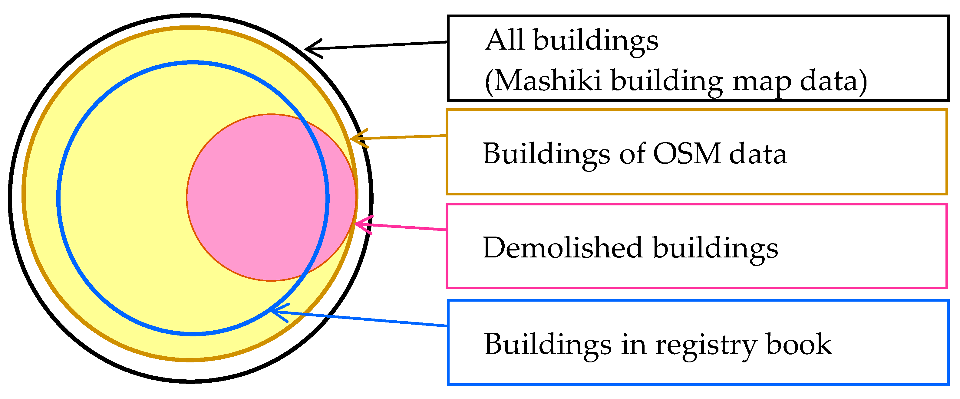
Remotesensing 11 02190 g004
Figure 5. Euler diagram of coverage of all buildings, buildings of the OSM data, demolished buildings, and buildings in the registry book of Mashiki administration.
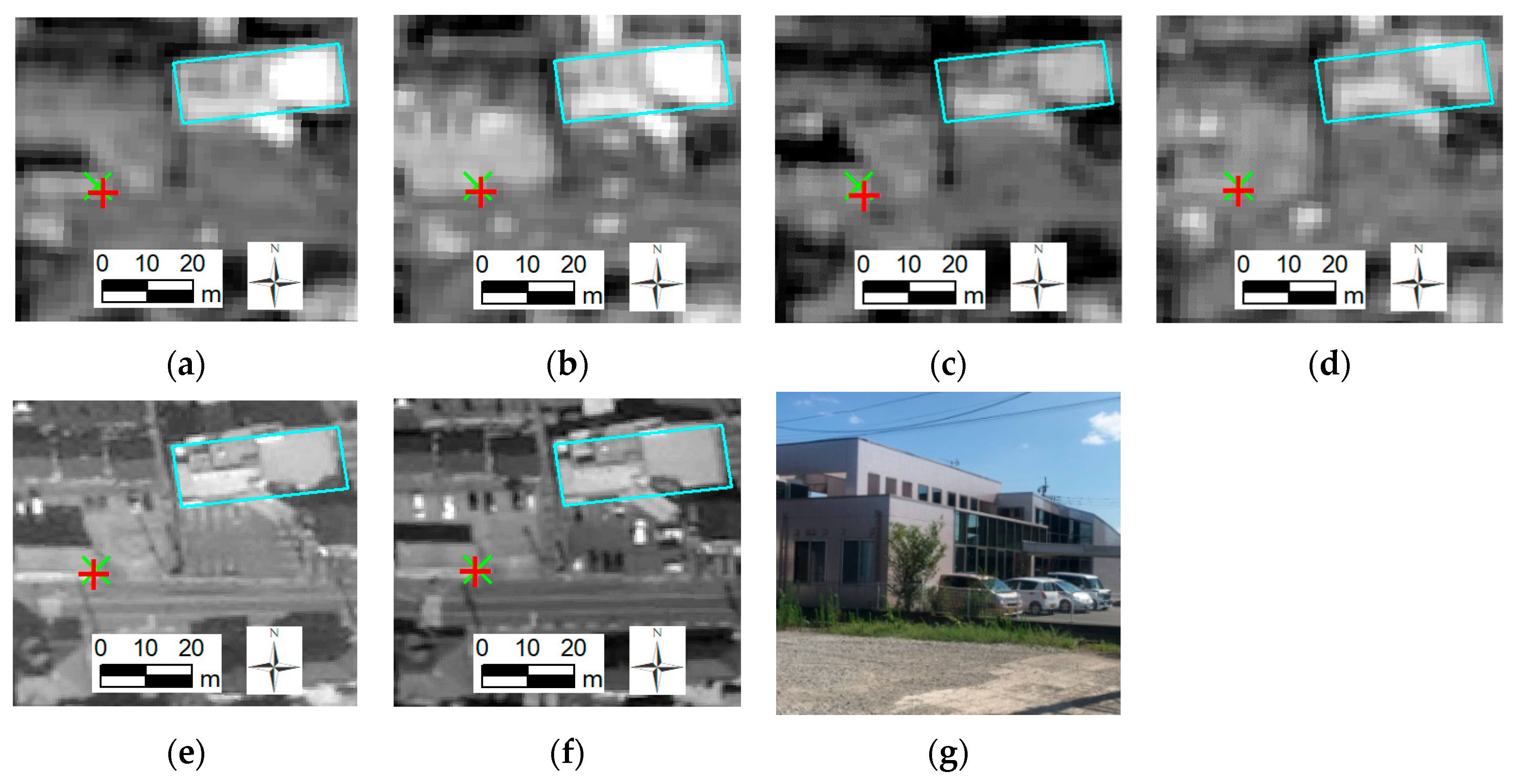
Remotesensing 11 02190 g005
Figure 6. Geometric evaluation of the orthorectified satellite imagery data. The GPS measured position (green X), the position of the building corner in images (red +), and the building footprint of the OSM data is overlaid on a (a) SPOT image on 20 March 2016; (b) SPOT image on 29 July 2016; (c) SPOT image on 1 January 2017; (d) SPOT image on 25 March 2018; (e) Pleiades image on 1 January 2017; and (f) Pleiades image on 13 October 2018. (g) Picture of the building from the position that the GPS measured toward the building outlined footprint of the OSM data.
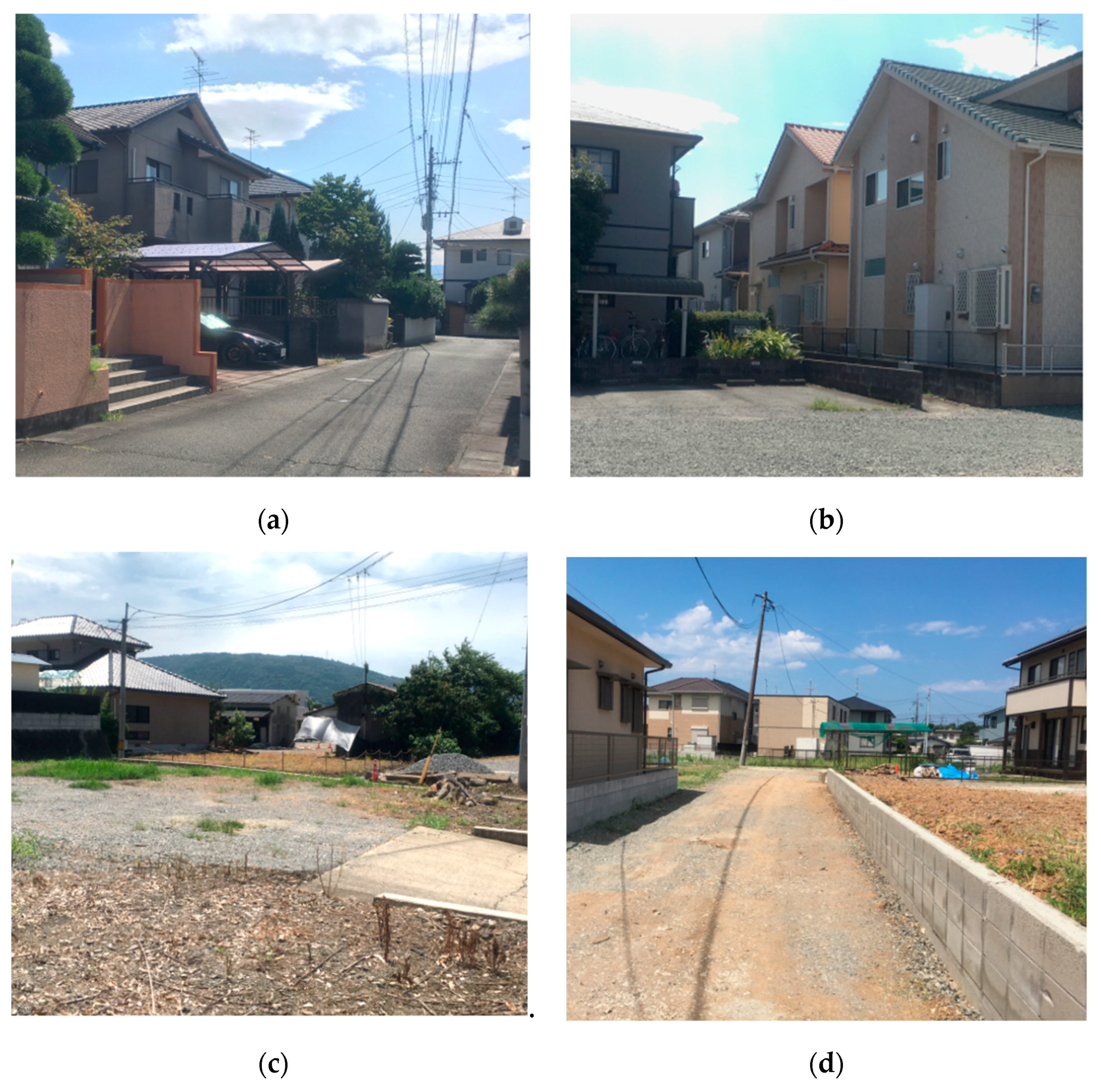
Remotesensing 11 02190 g006
Figure 7. Photos taken at arrow positions (ad) shown in Figure 8.
Remotesensing 11 02190 g007
Figure 8. Dataset polygon to establish a model by field survey of the area with a background image of Pleiades observed on 1 January 2017. Arrow positions (ad) of sample photos in Figure 7.
Remotesensing 11 02190 g008
Figure 9. Distribution and average of the digital number (DN) within the building footprints of OSM data from SPOT images observed on: (a) 20 March 2016; (b) 29 July 2017; (c) 1 January 2017; and (d) 25 March 2018.
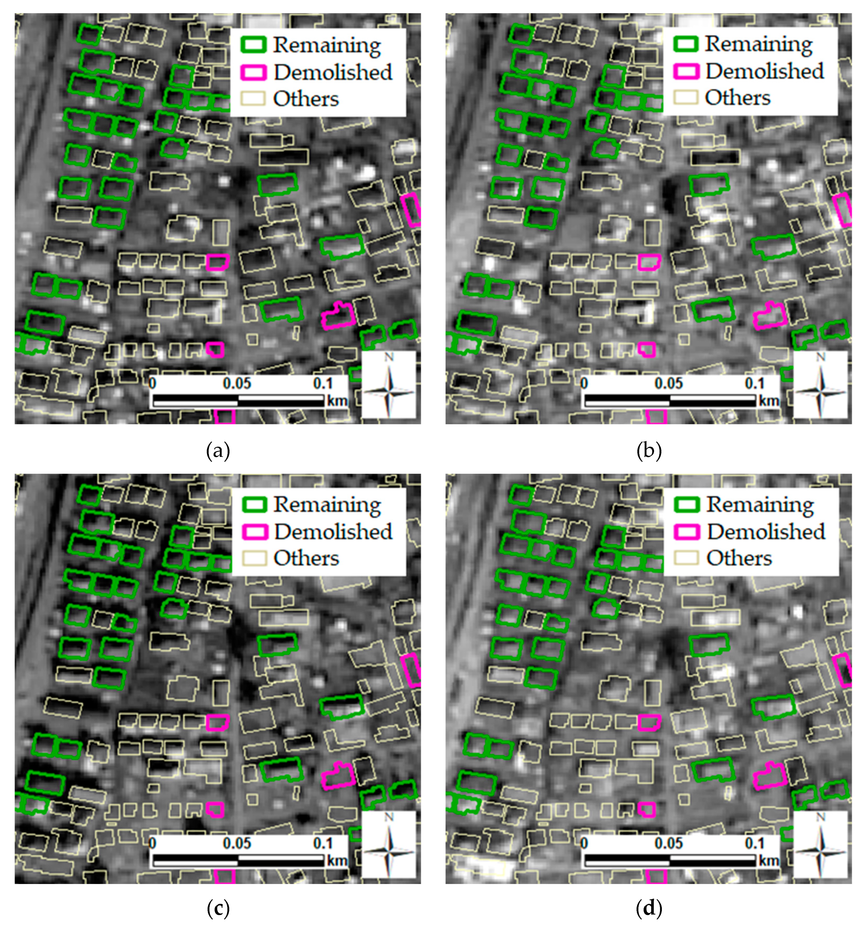
Remotesensing 11 02190 g009
Figure 10. Training data with labels of demolished and remaining buildings and background image of SPOT observed on: (a) 20 March 2016; (b) 29 July 2016; (c) 1 January 2017; and (d) 25 March 2018.
Remotesensing 11 02190 g010
Figure 11. Binary images calculated from: (a) 20 March 2016; (b) 29 July 2016; (c) 1 January 2017; and (d) 25 March 2018.
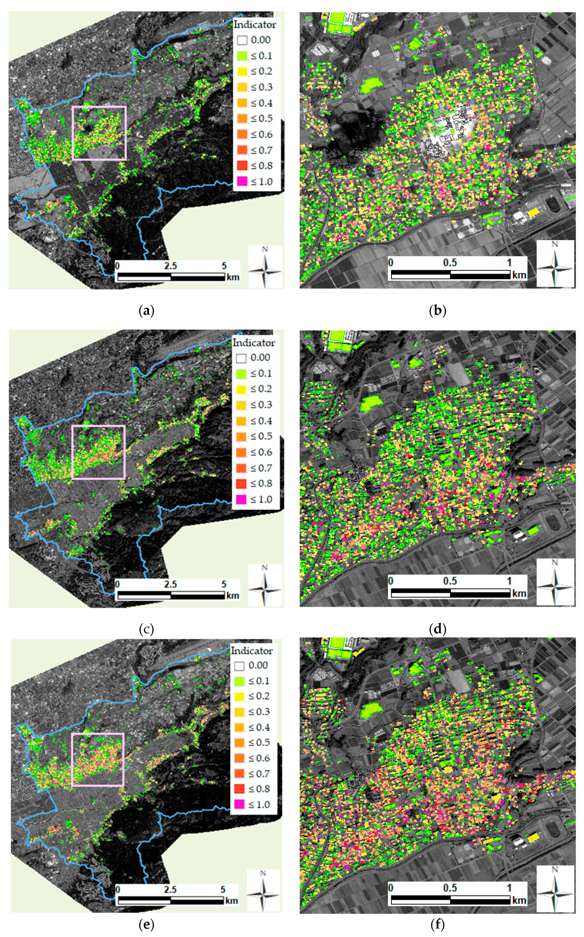
Remotesensing 11 02190 g011
Figure 12. Indicator distribution map: (a) Result from 20 March 2016 SPOT image; (c) result from 1 January 2017 SPOT image; (e) result from 25 March 2018 SPOT image; and (b,d,f) zoomed-in views of the rectangle area for each result.
Remotesensing 11 02190 g012
Figure 13. Receiver operating characteristics (ROC) curve for the true positive (TP) rate against the false positive (FP) rate based on the indicator and the training dataset with 110 labels in the Mashiki building map data.
Remotesensing 11 02190 g013
Figure 14. Visual interpretation of the indicator distribution map with transparent colors the same as Figure 12. (a) 20 March 2016 SPOT image; (b) 1 January 2017 SPOT image; and (c) 1 January 2017 Pleiades image. (d) Result of demolished building polygons by visual interpretation in the light blue outline.
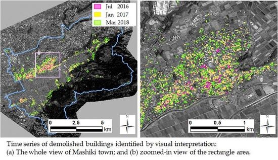
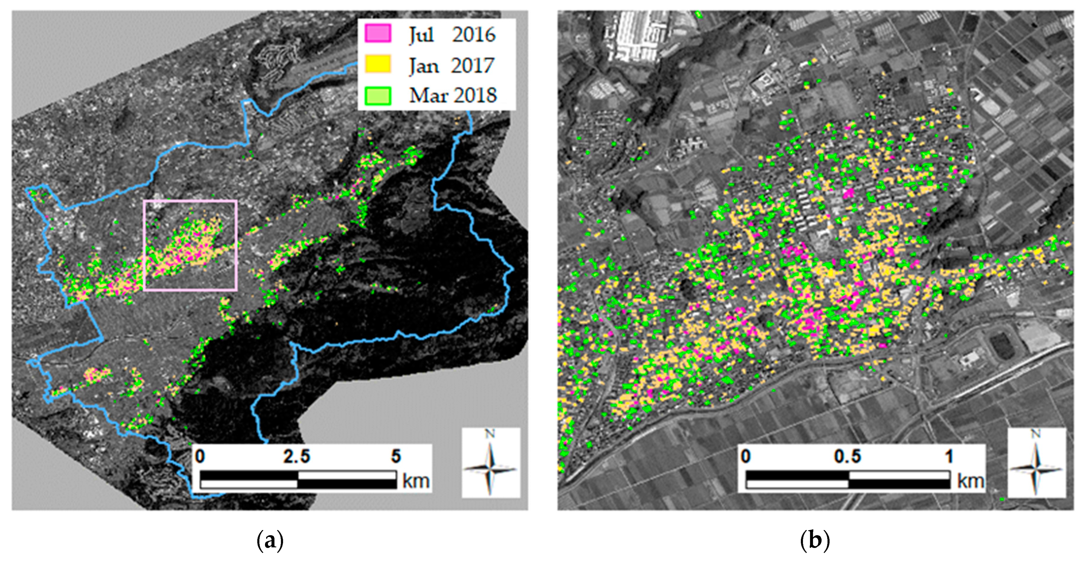
Remotesensing 11 02190 g014
Figure 15. Time series of demolished buildings identified by visual interpretation: (a) The whole view of Mashiki town; and (b) zoomed-in view of the rectangle area.
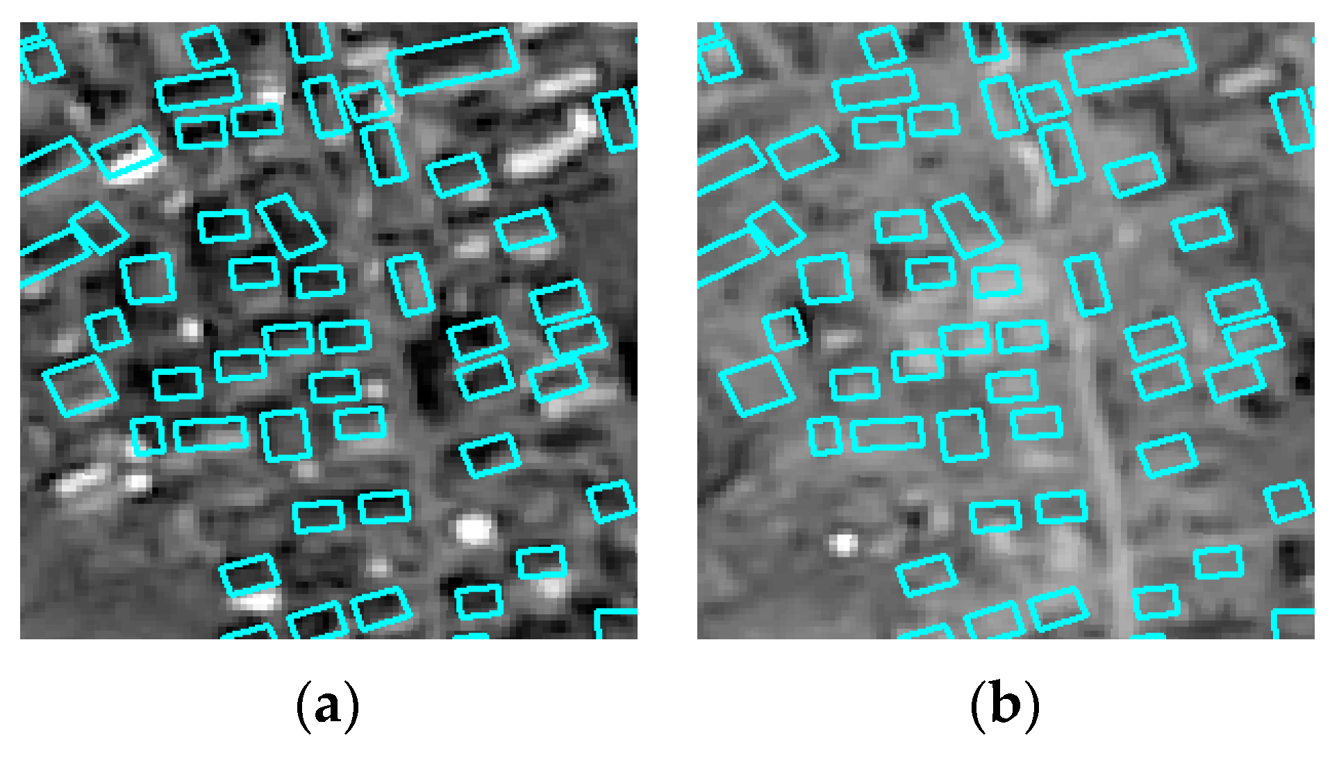
Remotesensing 11 02190 g015
Figure 16. Examples of the estimation of a TP by an indicator >0.3 drawn in blue outline on a: (a) 20 March 2016 SPOT image; and (b) 25 March 2018 SPOT image.
Remotesensing 11 02190 g016
Figure 17. Examples of the estimation of a true negative (TN) by indicator ≤0.3 drawn in blue outline on a: (a) 20 March 2016 SPOT image; and (b) 25 March 2018 SPOT image.
Remotesensing 11 02190 g017
Figure 18. Examples of the wrong estimation of a FP due to anomalous bright pixels drawn in blue outline on a: (a) 20 March 2016 SPOT image; and (b) 25 March 2018 SPOT image.
Remotesensing 11 02190 g018
Figure 19. Examples of positions and reflecting objects causing anomalous bright pixels: (a) 25 March 2016 SPOT image and arrows showing position for (bd) of Google Earth imageries [30]; (b) solar cell panels; (c) solar heating water tank; and (d) solar heating water tank.
Remotesensing 11 02190 g019
Figure 20. Examples of the estimation of a FP due to bright reflection from building walls drawn in blue outline on a: (a) 20 Mar 2016 SPOT image; and (b) 25 March 2018 SPOT image.
Remotesensing 11 02190 g020
Figure 21. Examples of the roof position shifted due to different view angles and tall buildings drawn in blue outline on a: (a) 20 March 2016 SPOT image; and (b) 25 March 2018 SPOT image.
Remotesensing 11 02190 g021
Figure 22. Examples of false negative (FN) estimation due to small areas of demolished buildings drawn in blue outline on a: (a) 20 March 2016 SPOT image; and (b) 25 March 2018 SPOT image.
Remotesensing 11 02190 g022
Table 1. List of satellite images selected in this research.
Observation DateSatellite NameResolutionIncidence Angle 1Usage
Along 2Across 3
20 March 2016SPOT-71.5 m−15.3−10.4Analysis
29 July 2016SPOT-61.5 m14.4−0.3Analysis
11 August 2016SPOT-71.5 m−18.27.0Interpolation
1 January 2017SPOT-61.5 m2.80.8Analysis
25 March 2018SPOT-71.5 m20.5−11.4Analysis
1 January 2017Pleiades-1B0.5 m7.411.6Interpretation
13 October 2018Pleiades-1B0.5 m13.56.5Interpretation
1 Incidence angle is the angle from the satellite to the center point of the image frame. 2 Incidence angle along the track is the angle between north and south (e.g., plus angle means looking from south, as the satellite direction is descending). 3 Incidence angle across the track is the angle between east to west (e.g., plus angle means looking from the west).
Table 2. Number of demolished and remaining buildings in the training dataset in the Mashiki building map data.
ClassNumber of Buildings
Demolished55
Remaining55
Total110
Table 3. Confusion matrix between estimated class and interpretation.
Estimation
DemolishedRemaining
Actual building situationDemolishedTrue Positive (TP)False Negative (FN)
RemainingFalse Positive (FP)True Negative (TN)
Table 4. Number of demolished buildings by our proposed method compared to the report of Mashiki municipality.
29 July 20161 January 201725 March 2018
Our proposed method23428375701
31 July 201631 December 201631 March 2018
Report of Mashiki administration21923955702
Table 5. F-measure by threshold for each observation date.
Threshold29 July 20161 January 201729 July 2016
0.00.748 0.743 0.688
0.10.887 0.908 0.780
0.20.940 0.955 0.864
0.30.965 0.962 0.920
0.40.954 0.942 0.906
0.50.922 0.911 0.857
0.60.900 0.842 0.778
0.70.675 0.659 0.571
0.80.533 0.429 0.429
0.90.226 0.167 0.226
Table 6. Confusion matrix by the indicator and threshold of 0.3 for 29 July 2016 image.
Estimation
DemolishedRemaining
InterpretationDemolished21816234
Remaining153214,12515,657
175014,14115,891 1
1 Does not include 215 buildings that were not classified due to shade and unclear images.
Table 7. Confusion matrix by the indicator and threshold of 0.3 for 1 January 2017 image.
Estimation
DemolishedRemaining
InterpretationDemolished147613612837
Remaining65312,42913,082
212913,79015,919 1
1 Does not include 187 buildings that were not classified due to shade and unclear images.
Table 8. Confusion matrix by the indicator and threshold of 0.3 for 25 March 2018 image.
Estimation
DemolishedRemaining
InterpretationDemolished268230195701
Remaining882926810,150
356412,28715,851 1
1 Does not include 255 buildings that were not classified due to shade and unclear images.
Table 9. Precision, recall, specificity, accuracy, and F-measure based on the confusion matrix for three image dates by the whole OSM dataset.
DatePrecisionRecallSpecificityAccuracyF-measure
29 July 20160.1250.9320.9020.9030.220
1 January 20170.6930.5200.9500.8730.594
25 March 20180.7530.4700.9130.7540.579
Table 10. Precision, recall, specificity, accuracy, and F-measure based on the confusion matrix for three image dates by the test dataset of 100 demolished and 100 remaining buildings.
DatePrecisionRecallSpecificityAccuracyF-measure
29 July 20160.0500.9400.9450.9490.940
1 January 20170.0200.8400.9030.9770.840
25 March 20180.0600.7900.8540.9290.790
Table 11. Relationship between the building area ≤60 m2 and the estimation classification by the indicator of 0.3 in the 25 March 2018 image.
Estimation
DemolishedRemaining
InterpretationDemolished5669571523
Remaining18420672251
75030243774
Table 12. Relationship between the building area >60 m2 of the footprint and true false of the estimation by the indicator of 0.3 in the 25 March 2018 image.
Estimation
DemolishedRemaining
InterpretationDemolished206420594123
Remaining69271527844
2756921111,967
Table 13. Precision, recall, specificity, accuracy, and F-measure based on the confusion matrixes of Table 11 and Table 12.
PrecisionRecallSpecificityAccuracyF-measure
Area ≤60 m20.7550.3720.9180.6980.498
Area >60 m20.7490.5010.9120.7700.600

