The Interannual Calibration and Global Nighttime Light Fluctuation Assessment Based on Pixel-Level Linear Regression Analysis


Abstract
:
1. Introduction
2. Data
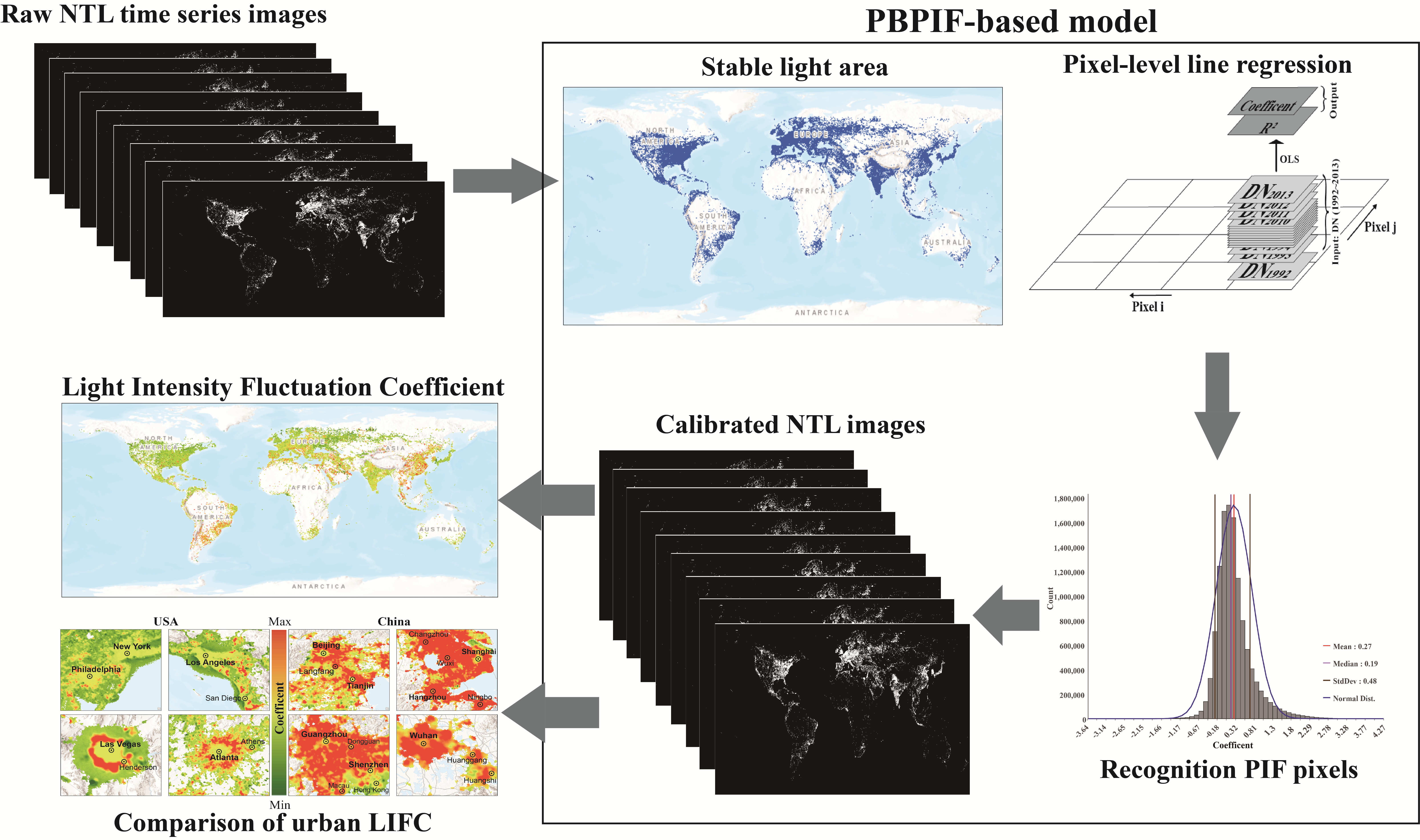
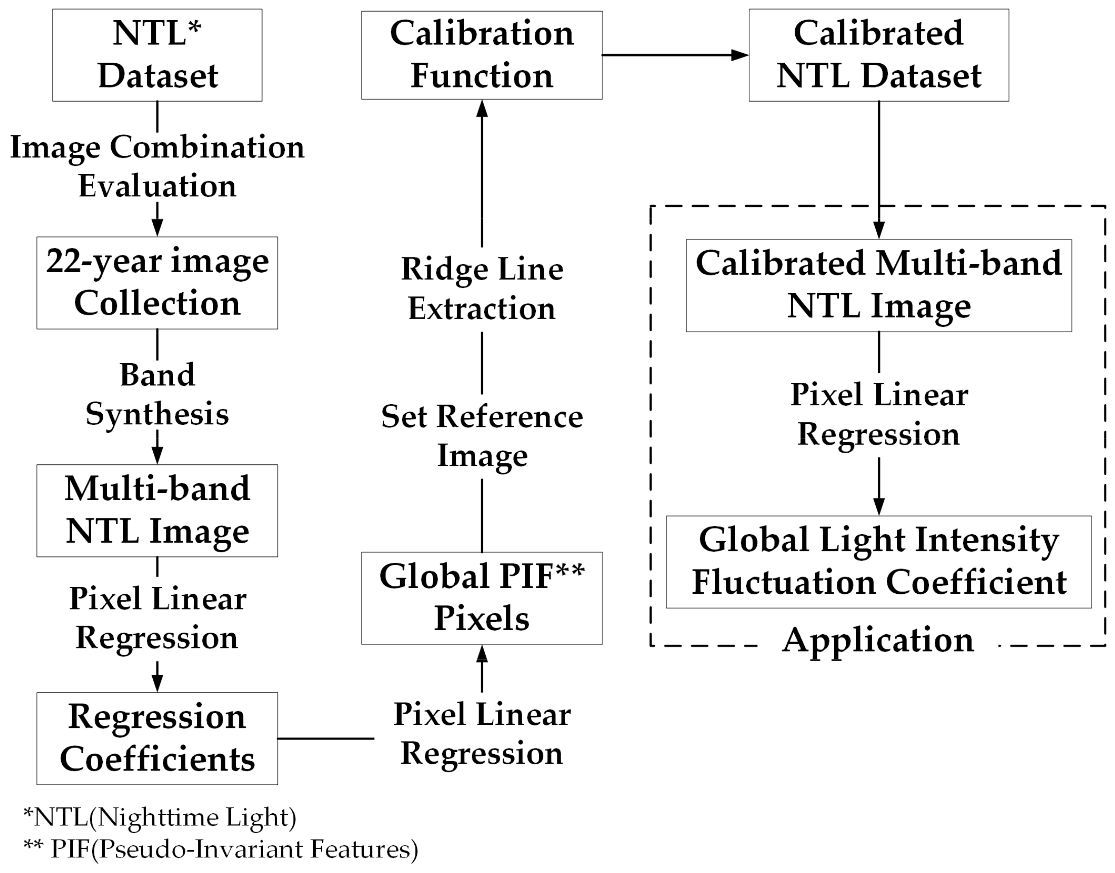
3. Methods
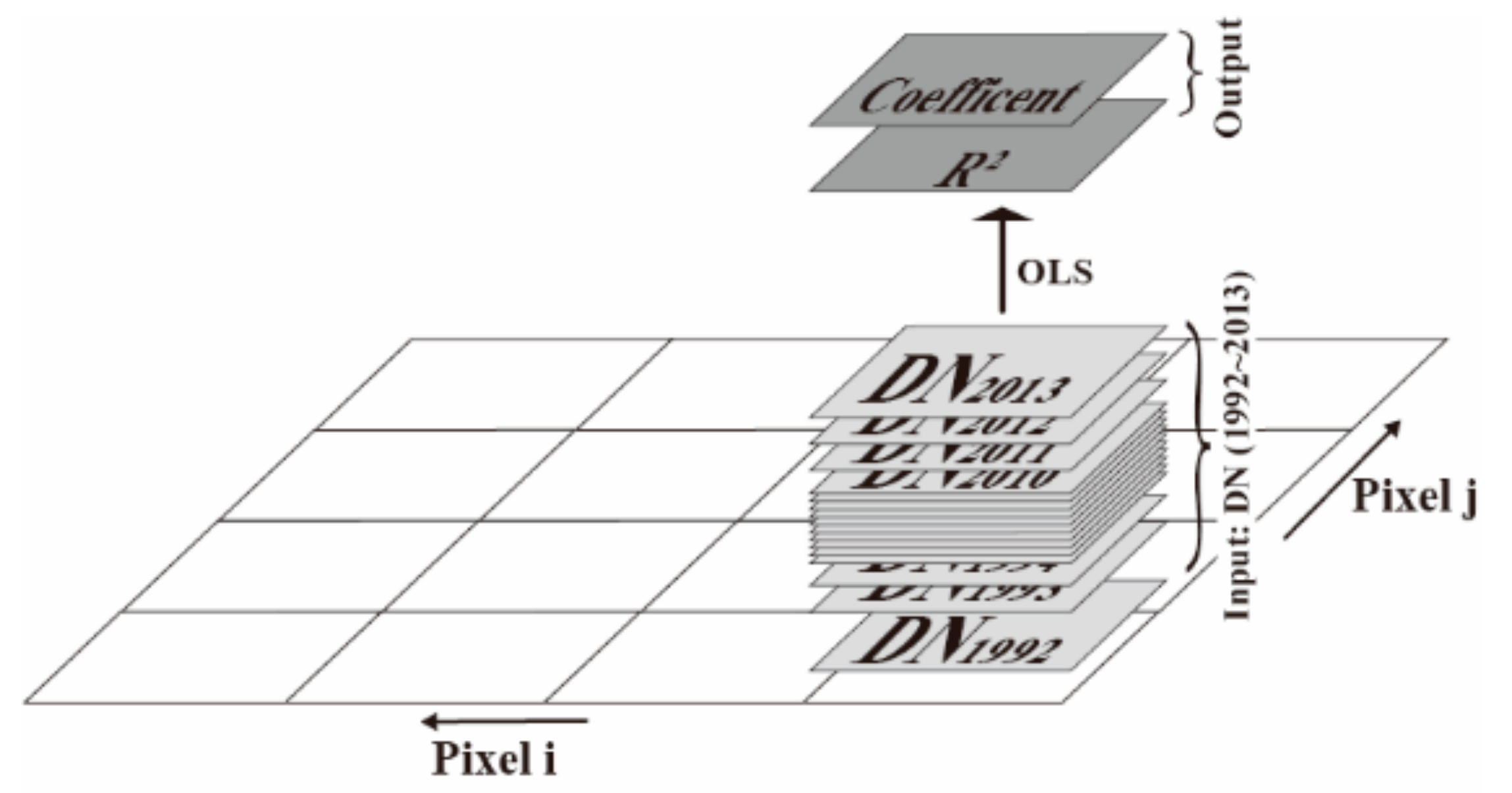
3.1. Interannual Calibration of DMSP/OLS NTL Time Series Datasets
3.1.1. Automatic Recognition of PIF
3.1.2. Reference Image Selection
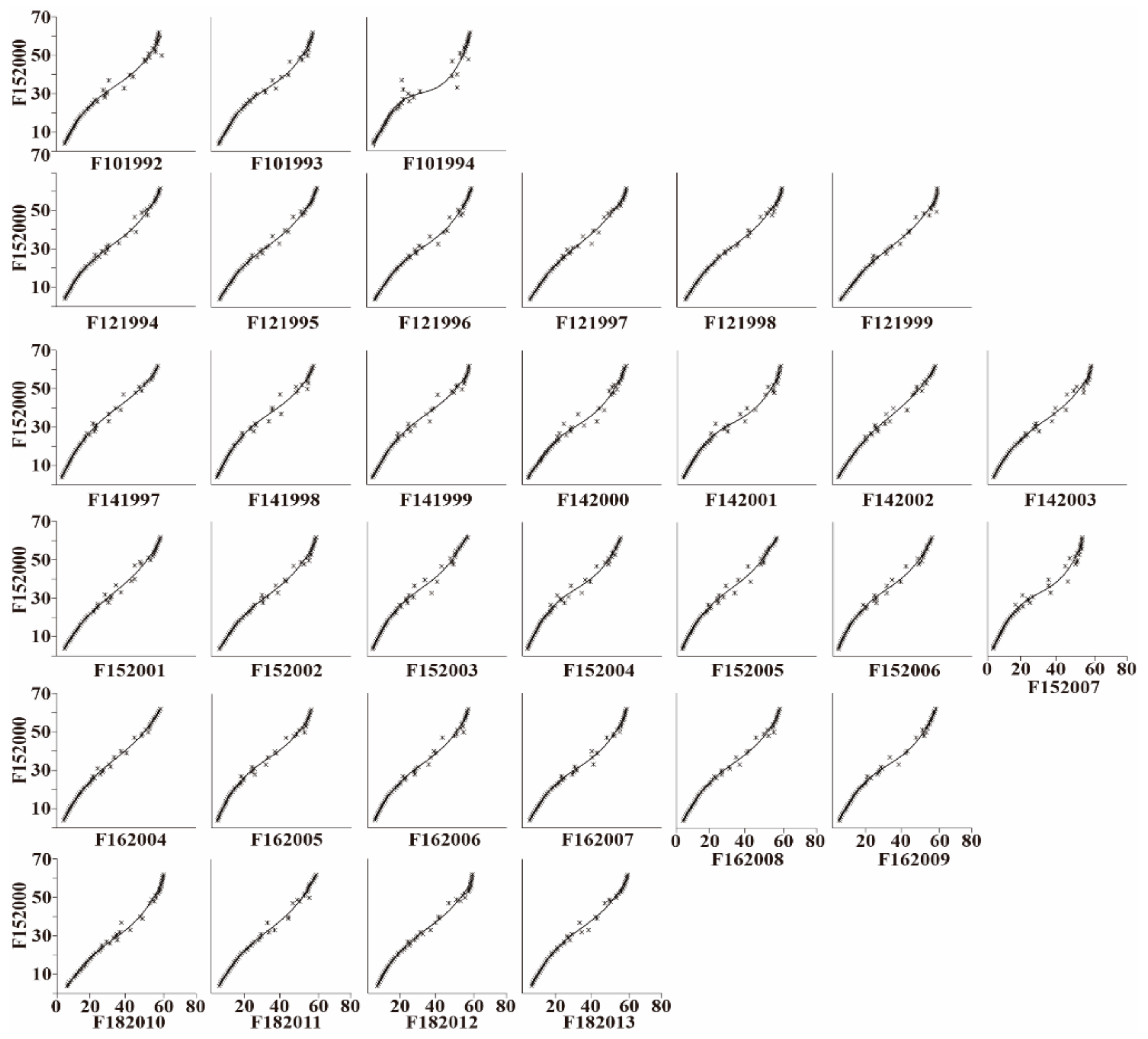
3.1.3. Calibration Function Setting
3.2. Evaluation of Calibration Results
3.3. Global Light Intensity Change Analysis
4. Results
4.1. Interannual Correction Results of NTL Datasets
4.2. Evaluation of Interannual Calibration Performance
4.2.1. PIF Recognition Results
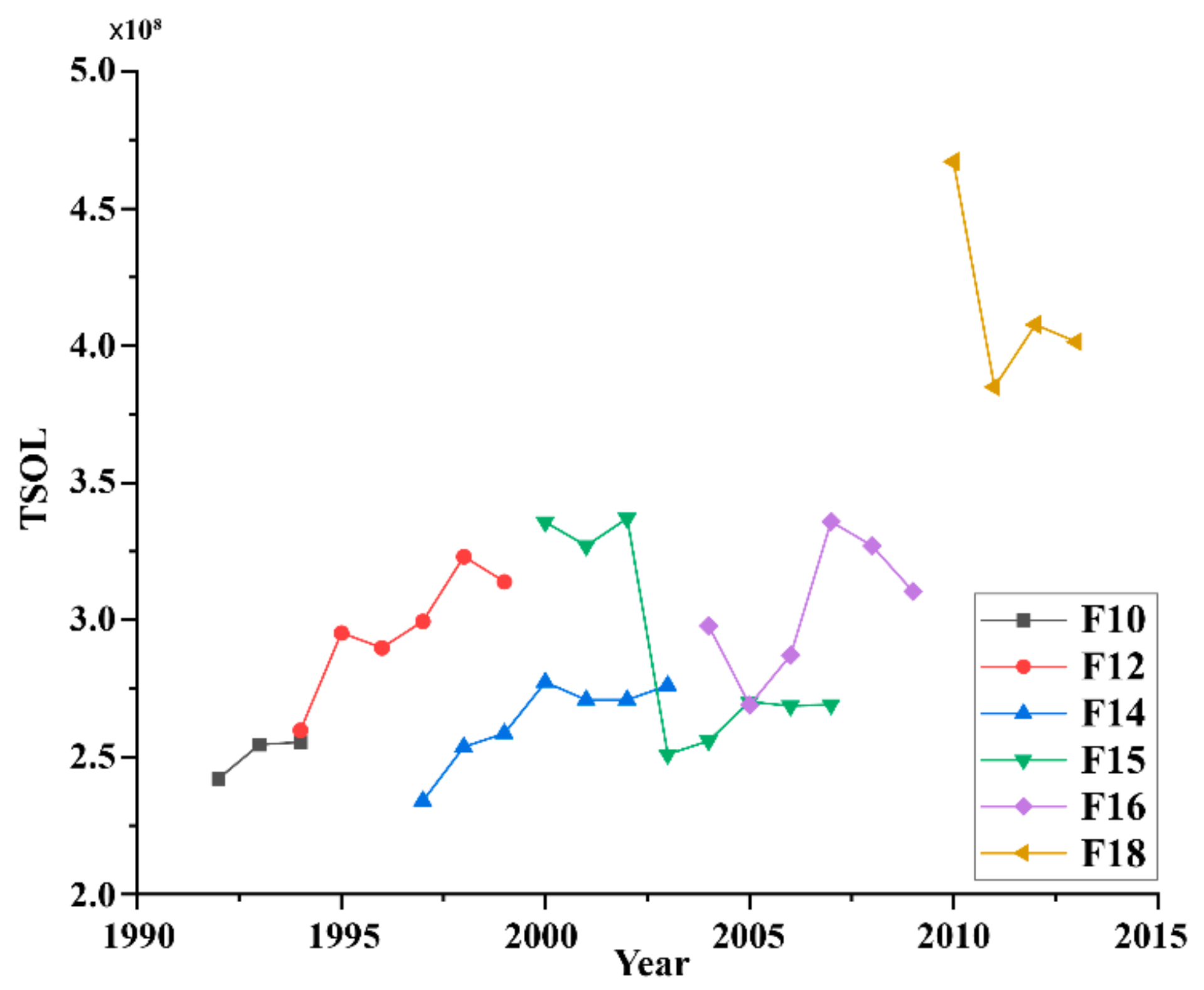
4.2.2. Global and regional TSOL continuity
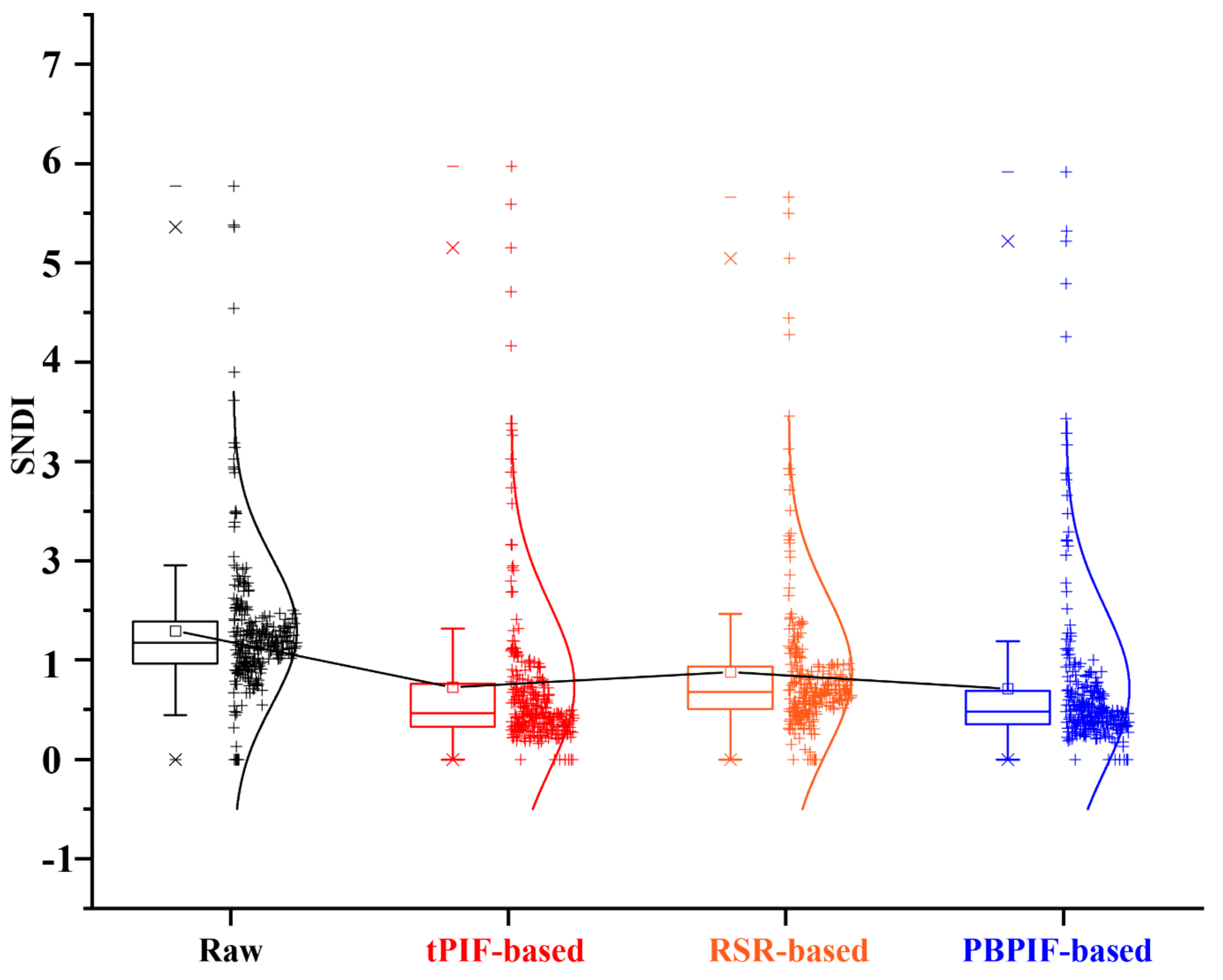
4.2.3. Comparison of SNDI
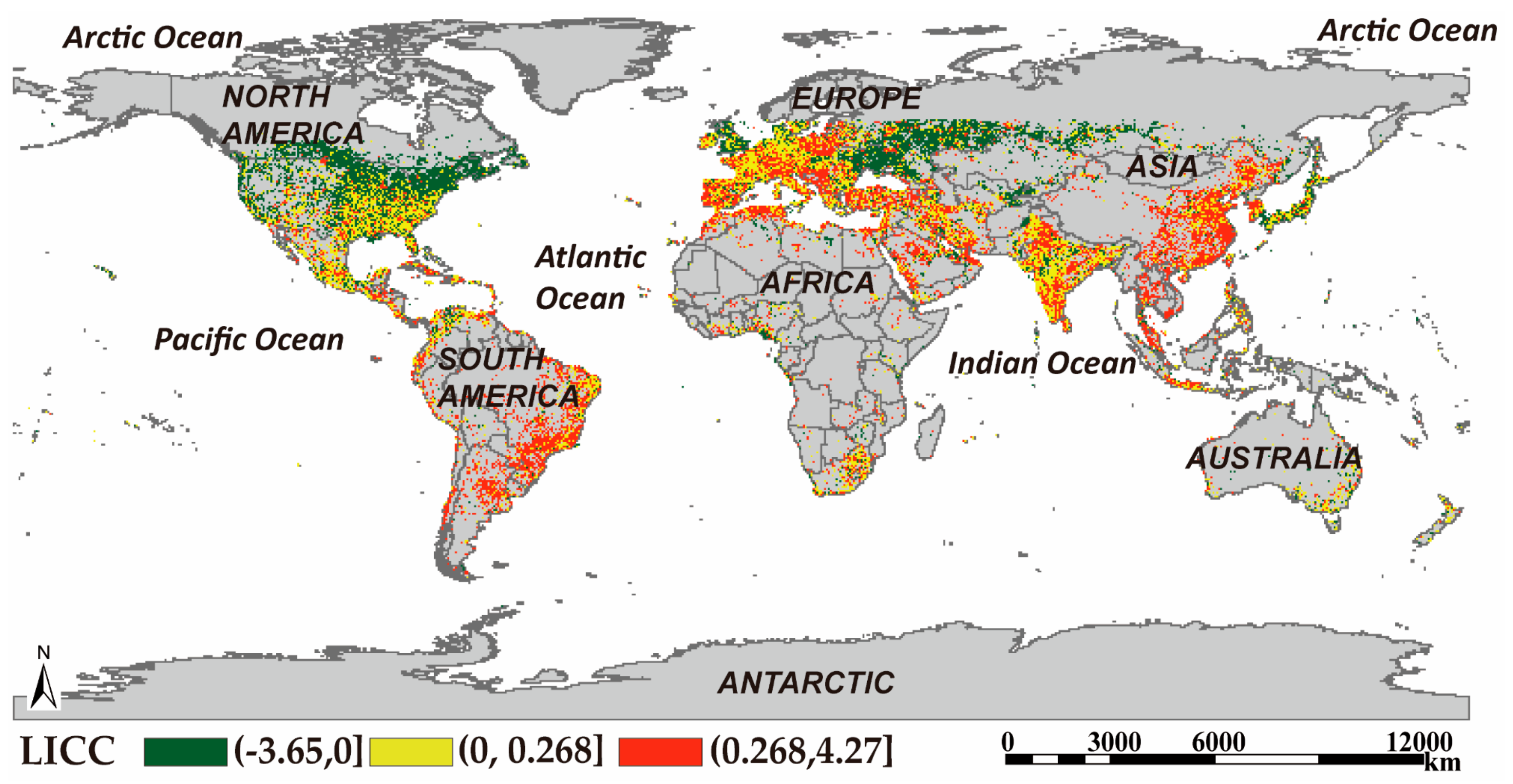
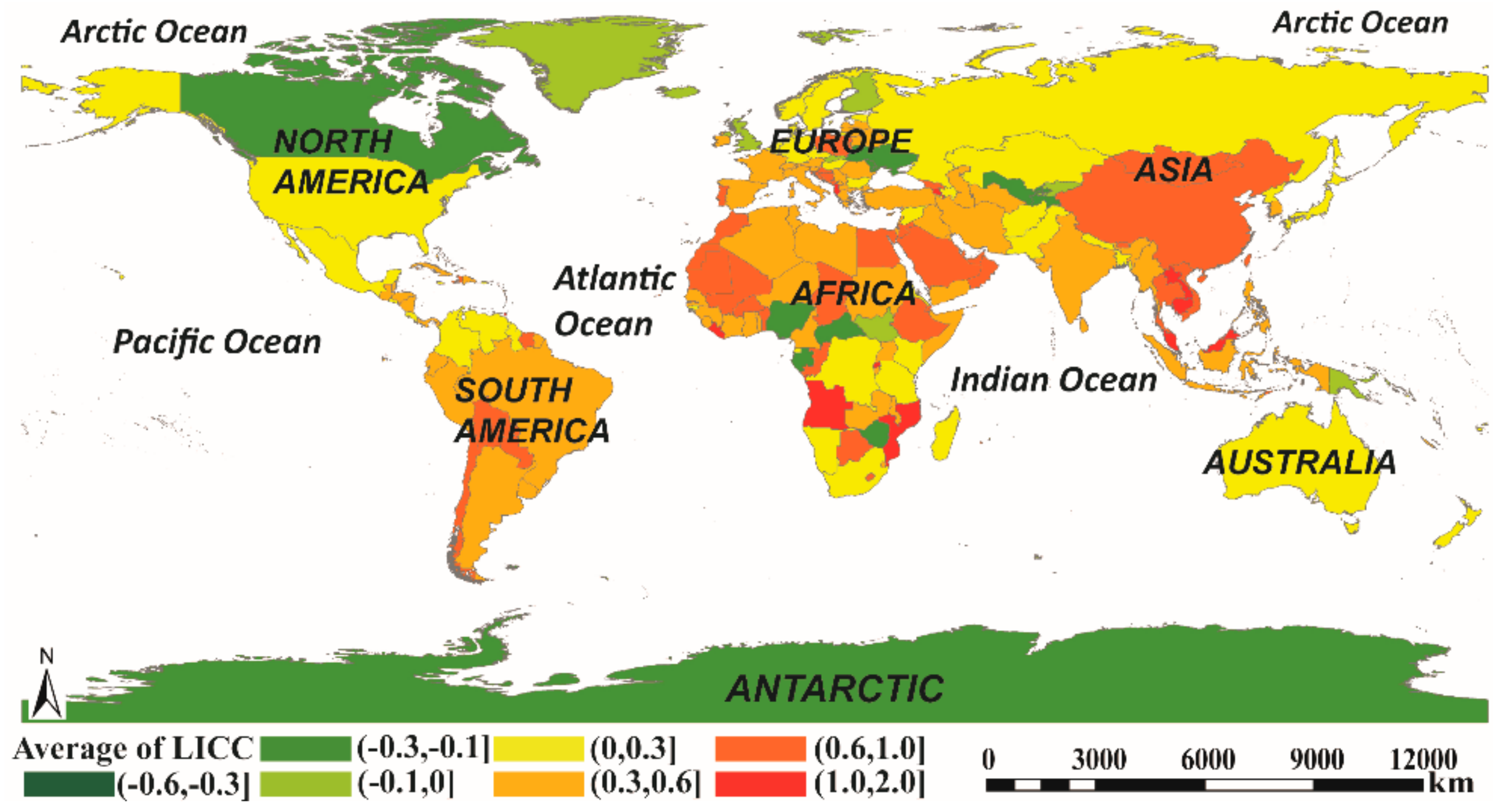
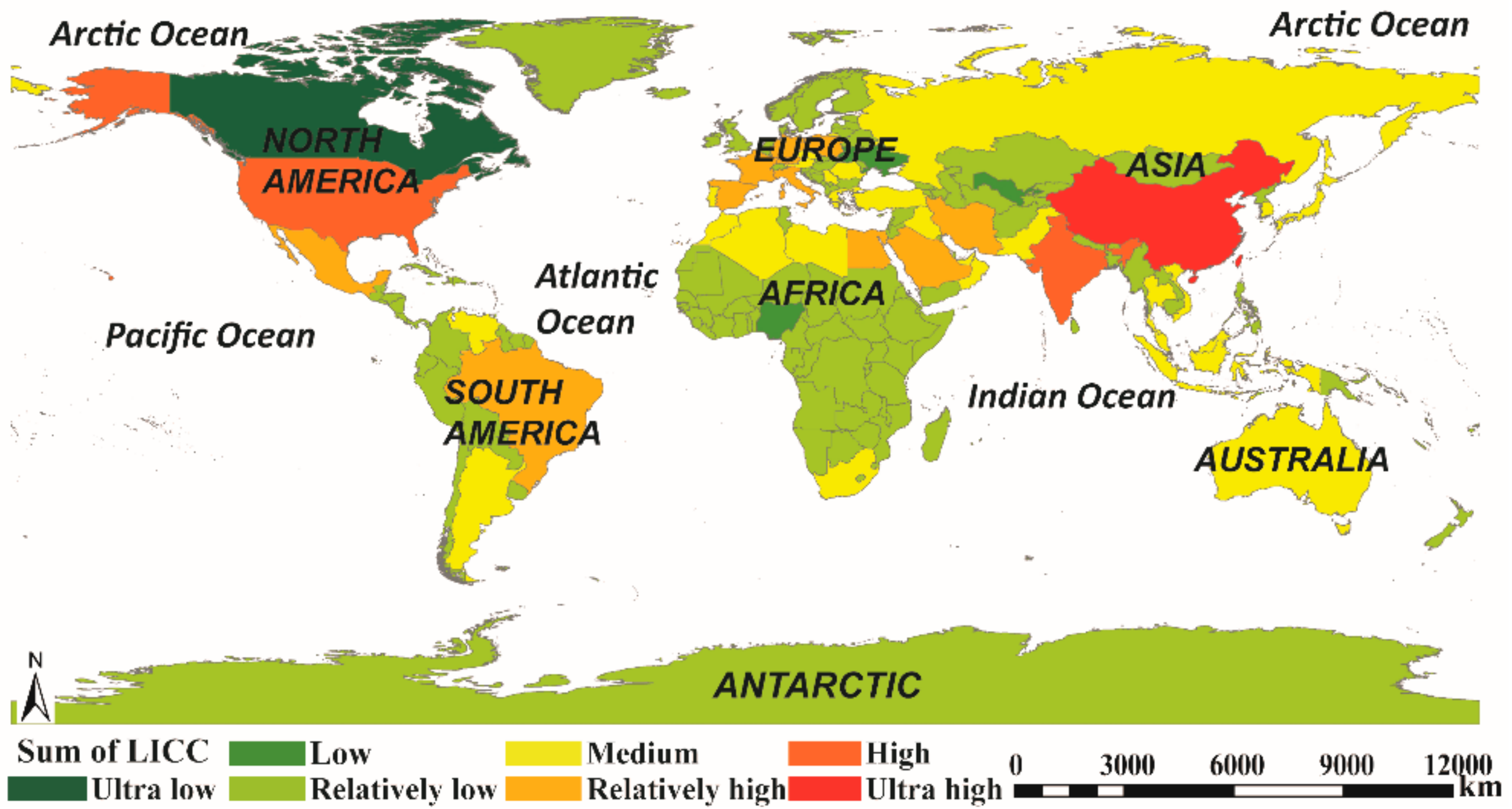
4.3. Global Night Lighting Intensity Changes
4.3.1. General Characteristics
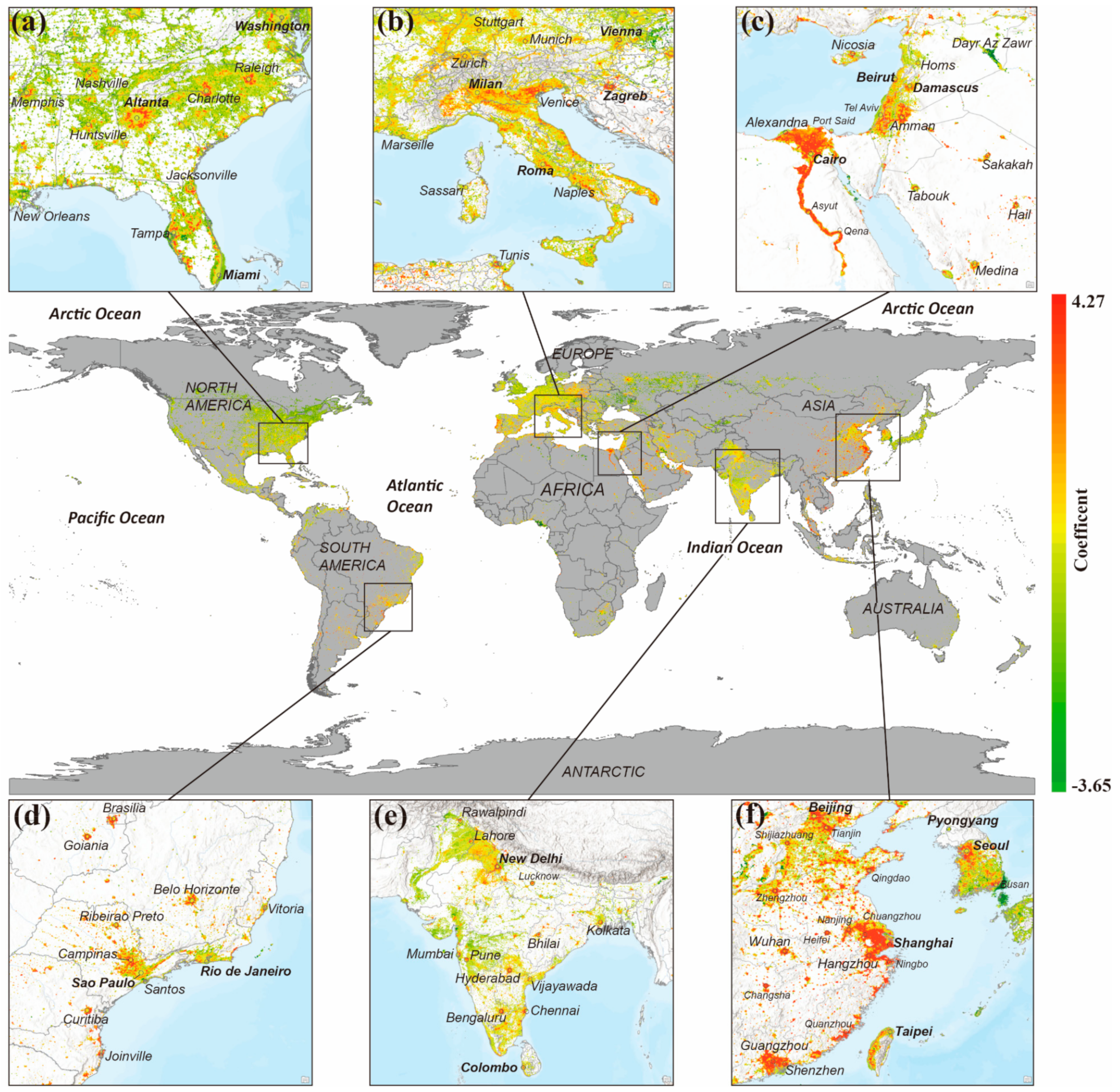
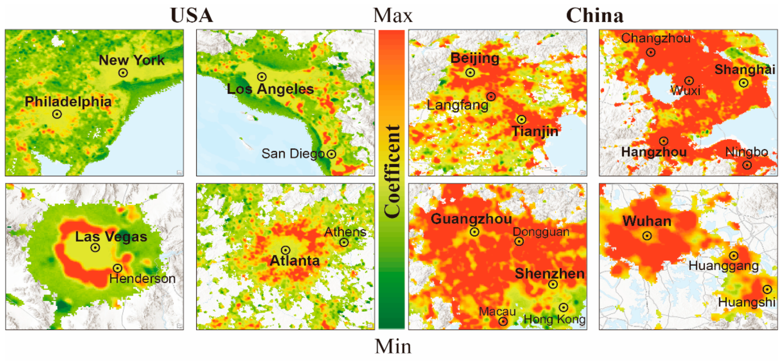
4.3.2. Regional Characteristics
5. Discussion
5.1. PBPIF-Based Calibration Model and Comparison of Results
5.2. Fluctuation Characteristics of NTL
6. Conclusions
Supplementary Materials
Author Contributions
Funding
Acknowledgments
Conflicts of Interest
References
- Croft, T.A. Nighttime images of the earth from space. Sci. Am. 1978, 239, 86–98. [Google Scholar] [CrossRef]
- Sutton, P.; Roberts, D.; Elvidge, C.; Meij, H. A comparison of nighttime satellite imagery and population density for the continental United States. Photogramm. Eng. Remote Sens. 1997, 63, 1303–1313. [Google Scholar]
- He, C.Y.; Shi, P.J.; Li, J.G.; Chen, J.; Pan, Y.Z.; Li, J.; Zhuo, L.; Ichinose, T. Restoring urbanization process in China in the 1990s by using non-radiance-calibrated DMSP/OLS nighttime light imagery and statistical data. Chin. Sci. Bull. 2006, 51, 1614–1620. [Google Scholar] [CrossRef]
- Lu, D.; Tian, H.; Zhou, G.; Ge, H. Regional mapping of human settlements in southeastern China with multisensor remotely sensed data. Remote Sens. Environ. 2008, 112, 3668–3679. [Google Scholar] [CrossRef]
- Ghosh, T.; Elvidge, C.D.; Sutton, P.C.; Baugh, K.E.; Ziskin, D.; Tuttle, B.T. Creating a global grid of distributed fossil fuel CO2 emissions from nighttime satellite imagery. Energies 2010, 3, 1895–1913. [Google Scholar] [CrossRef]
- Cao, Z.; Wu, Z.; Kuang, Y.; Huang, N.; Wang, M. Coupling an intercalibration of radiance-calibrated nighttime light images and land use/cover data for modeling and analyzing the distribution of GDP in Guangdong, China. Sustainability 2016, 8, 108. [Google Scholar] [CrossRef]
- Xie, Z.W.; Ye, X.Y.; Zheng, Z.H.; Li, D.; Sun, L.S.; Li, R.R.; Benya, S. Modeling Polycentric Urbanization Using Multisource Big Geospatial Data. Remote Sens. 2019, 11, 310. [Google Scholar] [CrossRef]
- Wu, K.; Wang, X. Aligning Pixel Values of DMSP and VIIRS Nighttime Light Images to Evaluate Urban Dynamics. Remote Sens. 2019, 11, 1463. [Google Scholar] [CrossRef]
- Zheng, Q.; Weng, Q.; Wang, K. Developing a new cross-sensor calibration model for DMSP-OLS and Suomi-NPP VIIRS night-light imageries. ISPRS J. Photogramm. Remote Sens. 2019, 153, 36–47. [Google Scholar] [CrossRef]
- Kyba, C.C.; Kuester, T.; De Miguel, A.S.; Baugh, K.; Jechow, A.; Hölker, F.; Bennie, J.; Elvidge, C.D.; Gaston, K.; Guanter, L. Artificially lit surface of Earth at night increasing in radiance and extent. Sci. Adv. 2017, 3, e1701528. [Google Scholar] [CrossRef] [Green Version]
- Elvidge, C.D.; Baugh, K.E.; Zhizhin, M.; Hsu, F.C. Why VIIRS data are superior to DMSP for mapping nighttime lights. In Proceedings of the Asia-Pacific Advanced Network 2013, Hawaii, OC, USA, 13–16 January 2013; Volume 35, p. 6. [Google Scholar]
- Miller, S.D.; Mill, S.P.; Elvidge, C.D.; Lindsey, D.T.; Lee, T.F.; Hawkins, J.D. Suomi satellite brings to light a unique frontier of nighttime environmental sensing capabilities. Proc. Natl. Acad. Sci. USA 2012, 109, 15706–15711. [Google Scholar] [CrossRef] [PubMed] [Green Version]
- Zhang, Q.; Pandey, B.; Seto, K.C. A robust method to generate a consistent time series from DMSP/OLS nighttime light data. IEEE Trans. Geosci. Remote Sens. 2016, 54, 5821–5831. [Google Scholar] [CrossRef]
- Ma, Q.; He, C.; Wu, J.; Liu, Z.; Zhang, Q.; Sun, Z. Quantifying spatiotemporal patterns of urban impervious surfaces in China: An improved assessment using nighttime light data. Landsc. Urban Plan. 2014, 130, 36–49. [Google Scholar] [CrossRef]
- Shao, Z.; Liu, C. The integrated use of DMSP-OLS nighttime light and MODIS data for monitoring large-scale impervious surface dynamics: A case study in the Yangtze River Delta. Remote Sens. 2014, 6, 9359–9378. [Google Scholar] [CrossRef]
- Pok, S.; Matsushita, B.; Fukushima, T. An easily implemented method to estimate impervious surface area on a large scale from MODIS time-series and improved DMSP-OLS nighttime light data. ISPRS J. Photogramm. Remote Sens. 2017, 133, 104–115. [Google Scholar] [CrossRef] [Green Version]
- Liao, B.; Wei, K.X.; Song, W.W. Assessment and application of DMSP/OLS nighttime light data in the spatial structure of urban system: A case of Jiangxi Province in nearly 16 years. Res. Environ. Yangtze Basin 2012, 21, 1295–1300. [Google Scholar]
- Ma, T.; Zhou, Y.; Zhou, C.; Haynie, S.; Pei, T.; Xu, T. Night-time light derived estimation of spatio-temporal characteristics of urbanization dynamics using DMSP/OLS satellite data. Remote Sens. Environ. 2015, 158, 453–464. [Google Scholar] [CrossRef]
- Yu, B.; Shu, S.; Liu, H.; Song, W.; Wu, J.; Wang, L.; Chen, Z. Object-based spatial cluster analysis of urban landscape pattern using nighttime light satellite images: A case study of China. Int. J. Geogr. Inf. Sci. 2014, 28, 2328–2355. [Google Scholar] [CrossRef]
- Sutton, P.C. 14 Estimation of Human Population Parameters Using Night-Time Satellite Imagery. In Remotely-Sensed Cities; Mesev, V., Ed.; CRC Press: Boca Raton, FL, USA, 2003; Volume 3, p. 301. [Google Scholar]
- Wu, J.; Wang, Z.; Li, W.; Peng, J. Exploring factors affecting the relationship between light consumption and GDP based on DMSP/OLS nighttime satellite imagery. Remote Sens. Environ. 2013, 134, 111–119. [Google Scholar] [CrossRef]
- Li, X.; Ge, L.; Chen, X. Detecting Zimbabwe’s decadal economic decline using nighttime light imagery. Remote Sens. 2013, 5, 4551–4570. [Google Scholar] [CrossRef]
- Xie, Y.; Weng, Q. Detecting urban-scale dynamics of electricity consumption at Chinese cities using time-series DMSP-OLS (Defense Meteorological Satellite Program-Operational Linescan System) nighttime light imageries. Energy 2016, 100, 177–189. [Google Scholar] [CrossRef]
- Bennett, M.M.; Smith, L.C. Advances in using multitemporal night-time lights satellite imagery to detect, estimate, and monitor socioeconomic dynamics. Remote Sens. Environ. 2017, 192, 176–197. [Google Scholar] [CrossRef]
- Huang, Q.; Yang, X.; Gao, B.; Yang, Y.; Zhao, Y. Application of DMSP/OLS nighttime light images: A meta-analysis and a systematic literature review. Remote Sens. 2014, 6, 6844–6866. [Google Scholar] [CrossRef]
- Pandey, B.; Zhang, Q.; Seto, K.C. Comparative evaluation of relative calibration methods for DMSP/OLS nighttime lights. Remote Sens. Environ. 2017, 195, 67–78. [Google Scholar] [CrossRef]
- Jensen, J.R.; Lulla, K. Introductory digital image processing: A remote sensing perspective. Geocarto Int. 1987, 2, 65. [Google Scholar] [CrossRef]
- Schott, J.R.; Salvaggio, C.; Volchok, W.J. Radiometric scene normalization using pseudoinvariant features. Remote Sens. Environ. 1988, 26, 1–16. [Google Scholar] [CrossRef]
- Tuttle, B.T.; Anderson, S.; Elvidge, C.; Ghosh, T.; Baugh, K.; Sutton, P. Aladdin’s magic lamp: Active target calibration of the DMSP OLS. Remote Sens. 2014, 6, 12708–12722. [Google Scholar] [CrossRef]
- Hall, F.G.; Strebel, D.E.; Nickeson, J.E.; Goetz, S.J. Radiometric rectification: Toward a common radiometric response among multidate, multisensor images. Remote Sens. Environ. 1991, 35, 11–27. [Google Scholar] [CrossRef]
- Elvidge, C.; Ziskin, D.; Baugh, K.; Tuttle, B.; Ghosh, T.; Pack, D.; Erwin, E.D.; Zhizhin, M. A fifteen year record of global natural gas flaring derived from satellite data. Energies 2009, 2, 595–622. [Google Scholar] [CrossRef]
- Elvidge, C.D.; Hsu, F.C.; Baugh, K.E.; Ghosh, T. National trends in satellite-observed lighting. Glob. Urban Monit. Assess. Earth Obs. 2014, 23, 97–118. [Google Scholar]
- Liu, Z.; He, C.; Zhang, Q.; Huang, Q.; Yang, Y. Extracting the dynamics of urban expansion in China using DMSP-OLS nighttime light data from 1992 to 2008. Landsc. Urban Plan. 2012, 106, 62–72. [Google Scholar] [CrossRef]
- Wu, J.; He, S.; Peng, J.; Li, W.; Zhong, X. Intercalibration of DMSP-OLS night-time light data by the invariant region method. Int. J. Remote Sens. 2013, 34, 7356–7368. [Google Scholar] [CrossRef]
- Hsu, F.C.; Baugh, K.E.; Ghosh, T.; Zhizhin, M.; Elvidge, C.D. DMSP-OLS radiance calibrated nighttime lights time series with intercalibration. Remote Sens. 2015, 7, 1855–1876. [Google Scholar] [CrossRef]
- Li, X.; Chen, X.; Zhao, Y.; Xu, J.; Chen, F.; Li, H. Automatic intercalibration of nighttime light imagery using robust regression. Remote Sens. Lett. 2013, 4, 45–54. [Google Scholar] [CrossRef]
- Pandey, B.; Joshi, P.K.; Seto, K.C. Monitoring urbanization dynamics in India using DMSP/OLS night time lights and SPOT-VGT data. Int. J. Appl. Earth Obs. Geoinf. 2013, 23, 49–61. [Google Scholar] [CrossRef]
- Bennie, J.; Davies, T.W.; Duffy, J.P.; Inger, R.; Gaston, K.J. Contrasting trends in light pollution across Europe based on satellite observed night time lights. Sci. Rep. 2014, 4, 3789. [Google Scholar] [CrossRef] [PubMed] [Green Version]
- Sánchez de Miguel, A.; Zamorano, J.; Castaño, J.G.; Pascual, S. Evolution of the energy consumed by street lighting in Spain estimated with DMSP-OLS data. J. Quant. Spectrosc. Radiat. Transf. 2014, 139, 109–117. [Google Scholar] [CrossRef] [Green Version]
- Ryan, R.E.; Pagnutti, M.; Burch, K.; Leigh, L.; Ruggles, T.; Cao, C.; Aaron, D.; Blonski, S.; Helder, D. The Terra Vega Active Light Source: A First Step in a New Approach to Perform Nighttime Absolute Radiometric Calibrations and Early Results Calibrating the VIIRS DNB. Remote Sens. 2019, 11, 710. [Google Scholar] [CrossRef]
- Song, C.; Woodcock, C.E.; Seto, K.C.; Lenney, M.P.; Macomber, S.A. Classification and change detection using Landsat TM data: When and how to correct atmospheric effects? Remote Sens. Environ. 2001, 75, 230–244. [Google Scholar] [CrossRef]
- Zhang, Q.; Seto, K.C. Mapping urbanization dynamics at regional and global scales using multi-temporal DMSP/OLS nighttime light data. Remote Sens. Environ. 2011, 115, 2320–2329. [Google Scholar] [CrossRef]
- Cauwels, P.; Pestalozzi, N.; Sornette, D. Dynamics and spatial distribution of global nighttime lights. EPJ Data Sci. 2014, 3, 2. [Google Scholar] [CrossRef] [Green Version]
- The World Band GDP (Current US$). Available online: https://data.worldbank.org/indicator/NY.GDP.MKTP.CD (accessed on 20 August 2019).
- Li, X.; Chen, F.; Chen, X. Satellite-observed nighttime light variation as evidence for global armed conflicts. IEEE J. Sel. Top. Appl. Earth Obs. Remote Sens. 2013, 6, 2302–2315. [Google Scholar] [CrossRef]
- Ma, T.; Zhou, C.H.; Pei, T.; Haynie, S.; Fan, J.F. Quantitative estimation of urbanization dynamics using time series of DMSP/OLS nighttime light data: A comparative case study from China’s cities. Remote Sens. Environ. 2012, 124, 99–107. [Google Scholar] [CrossRef]
- Ju, Y.; Dronova, I.; Ma, Q.; Zhang, X. Analysis of urbanization dynamics in mainland China using pixel-based night-time light trajectories from 1992 to 2013. Int. J. Remote Sens. 2017, 38, 6047–6072. [Google Scholar] [CrossRef]
- Zhang, X.; Guo, S.; Guan, Y.; Cai, D.; Zhang, C.; Fraedrich, K.; Xiao, H.; Tian, Z.Z. Urbanization and Spillover Effect for Three Megaregions in China: Evidence from DMSP/OLS Nighttime Lights. Remote Sens. 2018, 10, 1888. [Google Scholar] [CrossRef]
- Zhou, Y.; Li, X.; Asrar, G.R.; Smith, S.J.; Imhoff, M. A global record of annual urban dynamics (1992–2013) from nighttime lights. Remote Sens. Environ. 2018, 219, 206–220. [Google Scholar] [CrossRef]
- Chen, Z.; Yu, B.; Zhou, Y.; Liu, H.; Yang, C.; Shi, K.; Wu, J. Mapping Global Urban Areas From 2000 to 2012 Using Time-Series Nighttime Light Data and MODIS Products. IEEE J. Sel. Top. Appl. Earth Obs. Remote Sens. 2019, 12, 1143–1153. [Google Scholar] [CrossRef]
- Zheng, Z.; Yang, Z.; Wu, Z.; Marinello, F. Spatial Variation of NO2 and Its Impact Factors in China: An Application of Sentinel-5P Products. Remote Sens. 2019, 11, 1939. [Google Scholar] [CrossRef]
- Version 4 DMSP-OLS Nighttime Lights Time Series. Available online: https://ngdc.noaa.gov/eog/gcv4_readme.txt (accessed on 4 September 2019).
- Khawar, M. North Versus South—An Examination of Regional Comparative Development in Italy and Brazil. In The Geography of Underdevelopment; Palgrave Macmillan: Basingstoke, UK, 2017. [Google Scholar]
- Richmond, A.K. Water, Land, and Governance: Environmental Security in Dense Urban Areas in Sub-Saharan Africa. In The Environment-Conflict Nexus 2019; Springer: Cham, Switzerland, 2019. [Google Scholar]
- Eigenheer, D.M.; Somekh, N. Sao Paulo Metropolitan Transformations: Innovation or Reproduction. Urban. Reg. Plan. 2019, 4, 48. [Google Scholar] [CrossRef]
- Tan, K.G.; Luu, N.T.D.; Yoong Wei Cher, S. Understanding growth slowdown dynamics in India’s sub-national economies: An empirical investigation. Int. J. Soc. Econ. 2019, 46, 429–453. [Google Scholar] [CrossRef]
- Zheng, Z.; Chen, Y.; Wu, Z.; Ye, X.; Guo, G.; Qian, Q. The desaturation method of DMSP/OLS nighttime light data based on vector data: Taking the rapidly urbanized China as an example. Int. J. Geogr. Inf. Sci. 2019, 33, 431–453. [Google Scholar] [CrossRef]
- Zhang, Y.Y.; Tian, F. Definition of Emerging Economies and their role in the global economic landscape. Int. Econ. Rev. 2010, 4, 7–26. [Google Scholar]
- Zheng, W.; Xu, W.; Chen, Y. Dynamic Evolution of Economic Network within Inter-Regional Urban Agglomerations: Based on the Urban Agglomerations of West Coast of Taiwan Straits, Yangtze River Delta and Pearl River Delta. Econ. Geogr. 2019, 39, 58–66. [Google Scholar]
- Coesfeld, J.; Anderson, S.; Baugh, K.; Elvidge, C.; Schernthanner, H.; Kyba, C. Variation of individual location radiance in VIIRS DNB monthly composite images. Remote Sens. 2018, 10, 1964. [Google Scholar] [CrossRef]


| Sensor | Year | y = ax3 + bx2 + cx + d | Adj.R2 | |||
|---|---|---|---|---|---|---|
| a | b | c | d | |||
| F10 | 1992 | 0.0005 | −0.0512 | 2.3196 | −5.6617 | 0.985 |
| 1993 | 0.0006 | −0.0593 | 2.4654 | −5.7124 | 0.994 | |
| 1994 | 0.001 | −0.0982 | 3.3487 | −8.7948 | 0.967 | |
| F12 | 1994 | 0.0005 | −0.0484 | 2.169 | −5.0818 | 0.995 |
| 1995 | 0.0004 | −0.0396 | 2.0380 | −5.1433 | 0.996 | |
| 1996 | 0.0005 | −0.0486 | 2.2144 | −5.3353 | 0.995 | |
| 1997 | 0.0004 | −0.0382 | 1.9484 | −4.2920 | 0.995 | |
| 1998 | 0.0004 | −0.0398 | 2.0398 | −5.8782 | 0.997 | |
| 1999 | 0.0003 | −0.0299 | 1.8015 | −4.7800 | 0.991 | |
| F14 | 1997 | 0.0004 | −0.0447 | 2.2826 | −3.1678 | 0.996 |
| 1998 | 0.0005 | −0.0519 | 2.3574 | −3.8349 | 0.991 | |
| 1999 | 0.0004 | −0.0429 | 2.2022 | −3.4844 | 0.992 | |
| 2000 | 0.0006 | −0.0565 | 2.3019 | −3.789 | 0.989 | |
| 2001 | 0.0007 | −0.0662 | 2.5309 | −4.3559 | 0.991 | |
| 2002 | 0.0003 | −0.0324 | 1.9512 | −2.2158 | 0.995 | |
| 2003 | 0.0004 | −0.0395 | 2.0087 | −2.3651 | 0.991 | |
| F15 | 2000 | 0 | 0 | 1.0000 | 0 | 1.000 |
| 2001 | 0.0004 | −0.0374 | 1.9148 | −4.1631 | 0.994 | |
| 2002 | 0.0004 | −0.0396 | 2.0486 | −5.3467 | 0.995 | |
| 2003 | 0.0006 | −0.0582 | 2.3813 | −2.0850 | 0.992 | |
| 2004 | 0.0007 | −0.0671 | 2.5810 | −2.7208 | 0.994 | |
| 2005 | 0.0005 | −0.0498 | 2.2629 | −2.2188 | 0.993 | |
| 2006 | 0.0006 | −0.0570 | 2.3323 | −1.6420 | 0.995 | |
| 2007 | 0.0008 | −0.0784 | 2.9209 | −4.1009 | 0.987 | |
| F16 | 2004 | 0.0004 | −0.0396 | 2.0524 | −3.3894 | 0.997 |
| 2005 | 0.0006 | −0.0583 | 2.4086 | −2.7747 | 0.995 | |
| 2006 | 0.0005 | −0.0491 | 2.2482 | −2.8847 | 0.994 | |
| 2007 | 0.0005 | −0.0483 | 2.2178 | −4.8194 | 0.995 | |
| 2008 | 0.0005 | −0.0479 | 2.2036 | −4.3790 | 0.995 | |
| 2009 | 0.0006 | −0.0580 | 2.4550 | −4.5812 | 0.996 | |
| F18 | 2010 | 0.0005 | −0.0455 | 2.0468 | −8.3139 | 0.994 |
| 2011 | 0.0004 | −0.0395 | 2.0682 | −5.7123 | 0.995 | |
| 2012 | 0.0004 | −0.0411 | 2.1747 | −7.1854 | 0.995 | |
| 2013 | 0.0005 | −0.0480 | 2.2920 | −6.9268 | 0.996 | |
© 2019 by the authors. Licensee MDPI, Basel, Switzerland. This article is an open access article distributed under the terms and conditions of the Creative Commons Attribution (CC BY) license (http://creativecommons.org/licenses/by/4.0/).
Share and Cite
Zheng, Z.; Yang, Z.; Chen, Y.; Wu, Z.; Marinello, F. The Interannual Calibration and Global Nighttime Light Fluctuation Assessment Based on Pixel-Level Linear Regression Analysis. Remote Sens. 2019, 11, 2185. https://doi.org/10.3390/rs11182185
Zheng Z, Yang Z, Chen Y, Wu Z, Marinello F. The Interannual Calibration and Global Nighttime Light Fluctuation Assessment Based on Pixel-Level Linear Regression Analysis. Remote Sensing. 2019; 11(18):2185. https://doi.org/10.3390/rs11182185
Chicago/Turabian StyleZheng, Zihao, Zhiwei Yang, Yingbiao Chen, Zhifeng Wu, and Francesco Marinello. 2019. "The Interannual Calibration and Global Nighttime Light Fluctuation Assessment Based on Pixel-Level Linear Regression Analysis" Remote Sensing 11, no. 18: 2185. https://doi.org/10.3390/rs11182185
APA StyleZheng, Z., Yang, Z., Chen, Y., Wu, Z., & Marinello, F. (2019). The Interannual Calibration and Global Nighttime Light Fluctuation Assessment Based on Pixel-Level Linear Regression Analysis. Remote Sensing, 11(18), 2185. https://doi.org/10.3390/rs11182185