Night on South Korea: Unraveling the Relationship between Urban Development Patterns and DMSP-OLS Night-Time Lights

Abstract

Using artificial light data measured from satellites has the potential to change research methods in geography and urban planning. The Defense Meteorological Satellite Program Optical Linescan System (DMSP-OLS) night-time light datasets provided consistent and valuable data sources for investigating urbanization processes. This study intends to empirically investigate the relationship between night-time lights, population, and urban development patterns. A novel protocol was developed to integrate heterogeneous datasets into a standardized unit of analysis. Multivariate mixed-effects models were applied to detect correlations within and between provinces in South Korea. To capture physical variations of urban development, four landscape metrics were used and tested in the analyses. Diminishing returns of night-time lights to population were found in all models. In single landscape metric models, all coefficients of landscape metrics were positively related to night-time lights. In combination models, the aggregation index (AI) was no longer statistically significant. The protocol developed in this study provides an effective way to create analytical units for integrating heterogeneous forms of data. Creating standardized units of analyses will make it possible for researchers to compare their results with other studies. Landscape metrics used in this study for capturing the composition and configuration of urban development patterns will enrich the discussion in the future.

1. Introduction

One of the main features characterizing urban areas is artificial lights from buildings, transportation facilities, and other infrastructure [1]. The Defense Meteorological Satellite Program Optical Linescan System (DMSP-OLS) night-time lights dataset provides consistent and valuable data sources for investigating urbanization processes [2]. The night-time light data has been deployed to identify various types of urban dynamics, including population size [3,4,5,6,7], population density [8], energy consumption and greenhouse gas emission [9,10], light pollution [11], disasters [12,13], and built environments [14,15]. Although the data have offered a unique opportunity to characterize urbanization with various perspectives, the data have been mainly used as a proxy for economic activity such as regional gross domestic product in previous studies [3,16,17,18,19,20,21,22]. In particular, the historical archive of night-time light data will provide a valuable time-series that could be used to investigate the temporal characteristics of economic development where obtaining accurate metrics on the economy at regular intervals is difficult, including in underdeveloped countries.

Urbanization typologies have mostly been based on population measures [23]. Urban scaling laws, or characteristics of cities related to city size, have been used to investigate the quantitative variation of cities’ characteristics during the past decade [24,25,26,27]. A strong association between city size and economic productivity seems to be a fundamental characteristic of modern urban economics [28]. Previous studies showed that larger urban agglomerations are more innovative and productive [29,30,31,32] and that population size is a primary factor in determining the intensity of economic activity in urban areas [26,33]. In this study, the association between night-time lights as a proxy for economic activity and city size was carefully investigated with scaling functions and disaggregated population data. In addition to demographic change, physical transformation of the landscape is a major characteristic of urbanization [34]. Many previous studies have been conducted to investigate landscape changes using remote sensing techniques and GIS data [35,36,37]. They found that human activities are significantly related to urban environments [34,38]. In our study, land cover data from the Land Cover Map (LCM, 2010) were used in the analysis to detect urban development patterns. Specifically, several landscape metrics were applied to quantify these patterns.

This study investigates the relationship between night-time lights, population, and urban development patterns. Our study differs from previous research in two aspects. First, many studies have attempted to examine the association between night-time lights and urban characteristics based on a spatial extent of the city [9,15,16,21]. In many cases, the unit of analysis used in the study was an administrative boundary of the city. However, since definitions of cities and methods to delineate the boundary of city are not consistent across regions and countries, comparisons of model results for estimating the association between night-time lights and urban characteristics were limited. We developed a unique protocol to integrate night-time lights, population, and urban development pattern datasets into a standardized unit of analysis. We applied multivariate mixed-effects models to reflect correlations within and between provinces in South Korea. Secondly, although studies have examined the relationship between night-time lights and physical transformation of the city [2,39], quantitative measures used to identify urban development patterns were limited. To capture physical variations of urban development, we tested several landscape metrics. With clear and replicable processes for modeling night-time lights, researchers could better understand and compare the characteristics of urbanization.

2. Materials and Methods

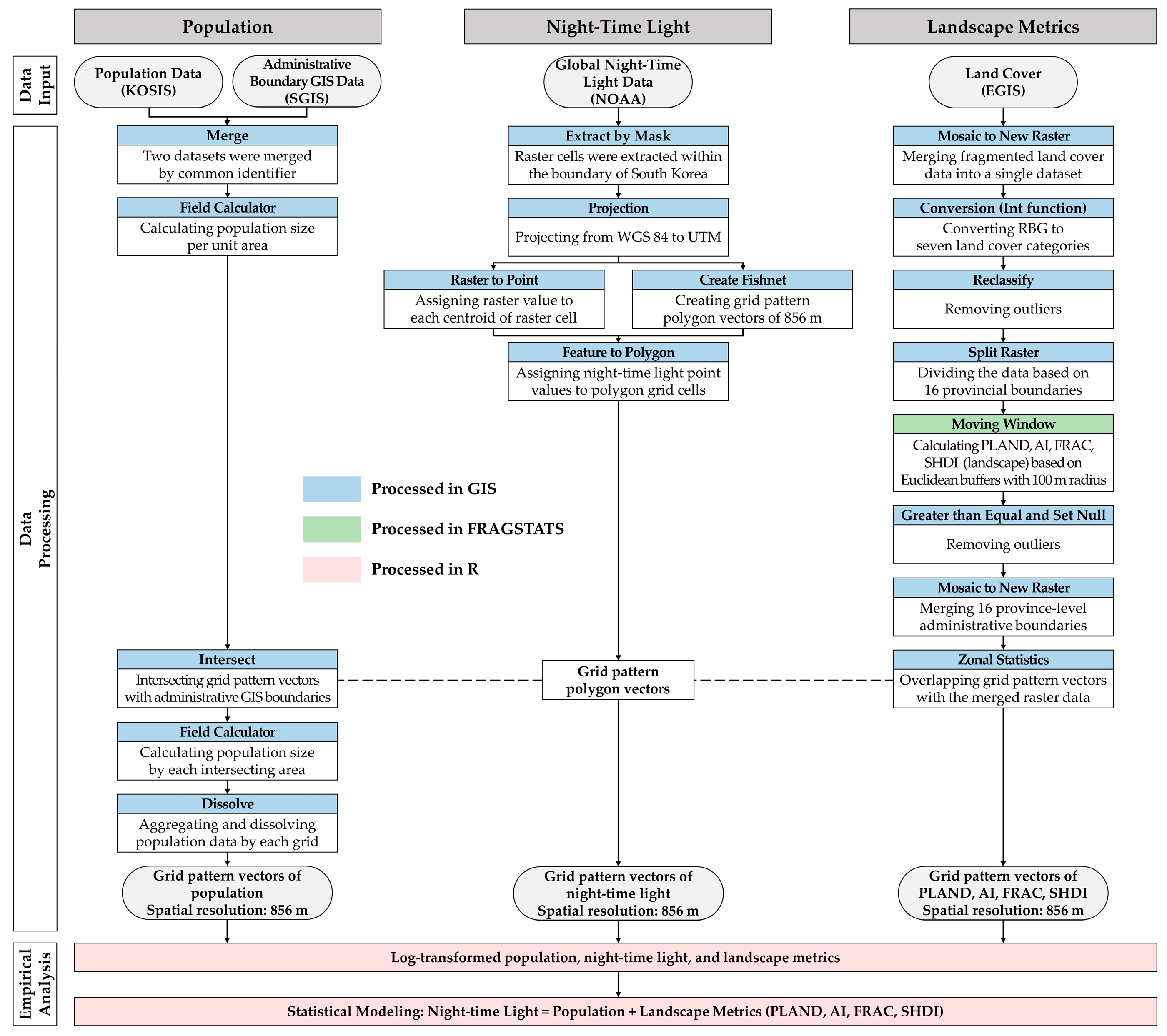
2.1. Data Sources and Measurement

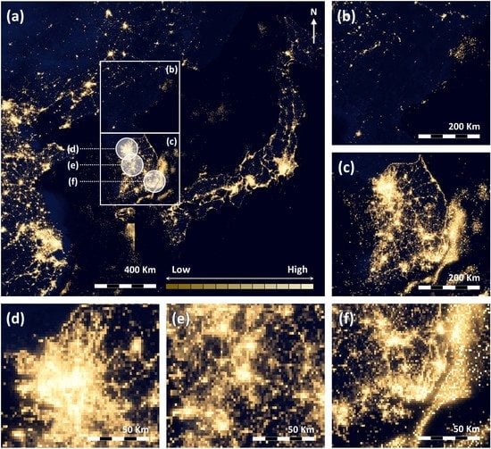
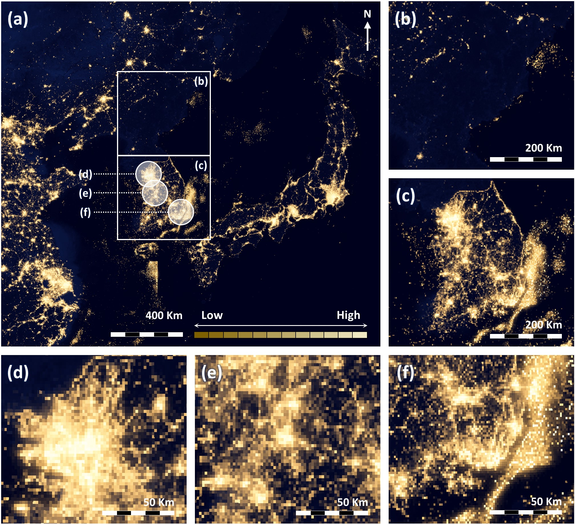
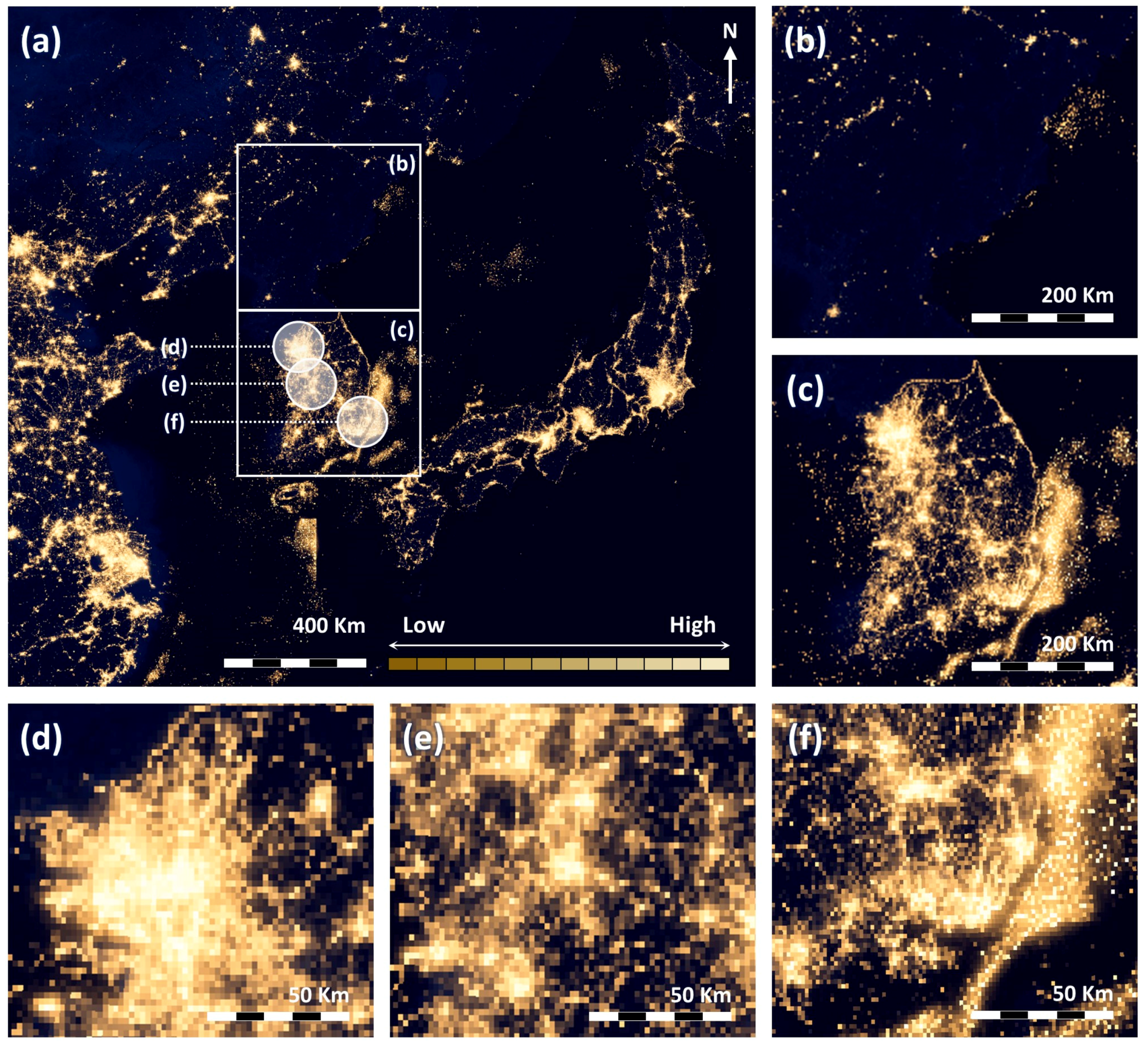
2.1.1. Night-Time Lights

The outcome of this study was DMSP-OLS stable night-time light data in 2010. The data were obtained from the National Centers for Environmental Information (NCEI) of the National Oceanic and Atmospheric Administration (NOAA); version 4 DMSP-OLS Nighttime Lights Time Series (downloaded on 25 November 2017). The original data were collected by the US Air Force Weather Agency. The raw data were produced based on 30 arcsec grids spanning −180° to 180° longitude, and −65° to 75° latitude. Sunlight and glare data were excluded based on the solar elevation angle. Moonlight data were excluded based on lunar illuminance calculation. Lighting features from the aurora were removed in the northern hemisphere on an orbit-by-orbit manner by visual inspection. Ephemeral events such as fires and observations with clouds were also excluded. These processes were conducted by NOAA’s National Geophysical Data Center. The data provided grid-cell based annual composite night-time light values (ranging from 1 to 63) from cities, towns and other sites with persistent lighting. Since the data values have a cap (value = 63), they were often saturated in the center of city areas.

Spatial patterns of night-time light data are shown in Figure 1. High nigh-time light values were observed in major cities in East Asian countries including Seoul, Busan, Beijing, Shanghai, and Tokyo (Figure 1a). Most cities in North Korea showed low-level night-time lights (Figure 1b) compared to other regions. High-level night-time lights were detected along the major corridor of South Korea (Figure 1c). Seoul (Figure 1d) and Busan (Figure 1f) showed the highest values and the most concentrated spatial patterns of night-time lights among major cities in the Korean peninsula.

2.1.2. Population

Population data were used as a predictor for estimating night-time lights in statistical models and were obtained from the Korean Statistical Information Service (KOSIS, 2010). Corresponding GIS boundary data were collected from the Statistical Geographic Information Service (SGIS, 2010). Two datasets were merged based on a common identifier at the neighborhood-level administrative unit (eup-myeon-dong). Area-weighted population values were calculated by intersecting administrative GIS layers with grid pattern polygon vectors (856 m × 856 m).

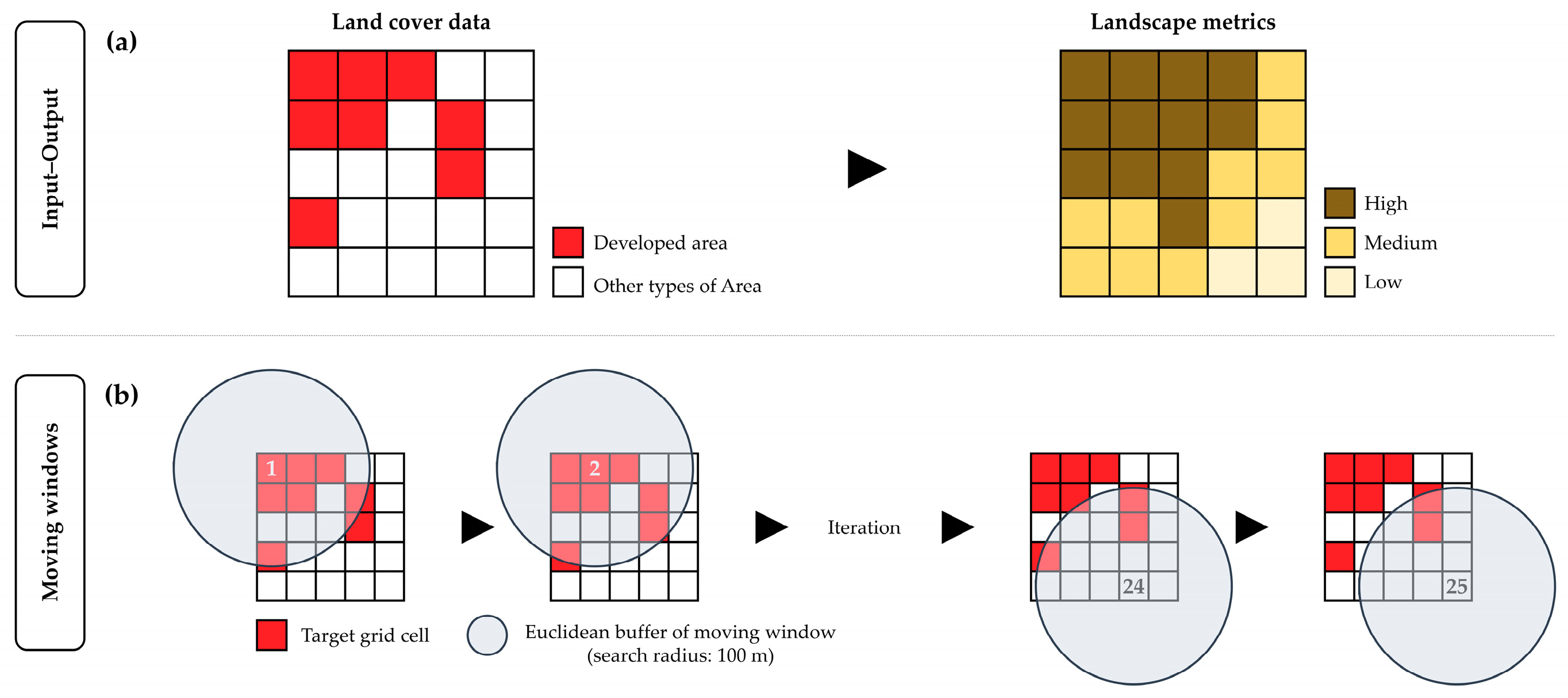
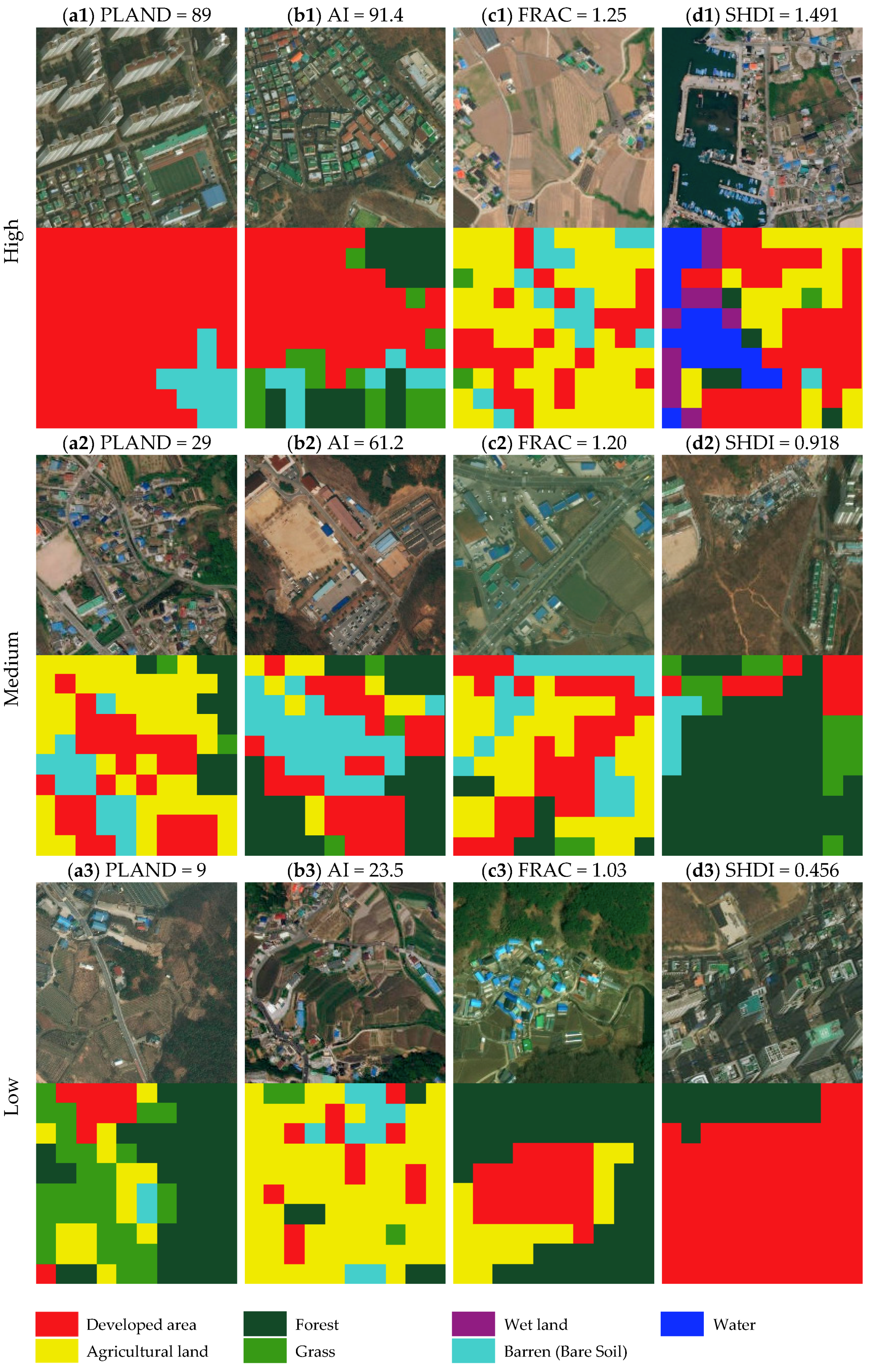
2.1.3. Landscape Metrics

Four landscape metrics were used to identify spatial patterns of the developed area and land cover diversity (

Table 1. Landscape metric equations used to detect spatial patterns of urbanization.

Metrics	Equation
Percentage of landscape (0 ≤ PLAND ≤ 100)	$$\begin{array}{c}\mathrm{PLAND}=\frac{{{\displaystyle \sum }}_{j=1}^n{P}_{ij}}{L}\left(100\right)\end{array}$$ (1) Pij = area of patch ij, L = total landscape area
Aggregation index (0 ≤ AI ≤ 100)	$$\begin{array}{c}\mathrm{AI}=\left[\frac{t_{ii}}{max\to t_{ii}}\right]\left(100\right)\end{array}$$ (2) tii = number of like adjacencies between grid cells of land cover type i max → tii = max number of like adjacencies between grid cells of land cover type i
Fractal dimension index (1 ≤ FRAC ≤ 2)	$$\begin{array}{c}\mathrm{FRAC}=\frac{2\ln \left(0.25s_{ij}\right)}{ln{d}_{ij}}\end{array}$$ (3) sij = perimeter of land cover grid ij, dij = area of land cover grid ij
Shannon’s diversity index (0 ≤ SHDI)	$$\begin{array}{c}\mathrm{SHDI}=-{\displaystyle \sum }_{i=1}^m{H}_{i}ln{H}_i\end{array}$$ (4) Hi = proportion of the landscape occupied by land cover type i

). First, percentage of landscape (PLAND) represents the proportion of the landscape occupied by a certain land cover type (Equation (1)). Since the developed area from land cover data was used as an input for calculating landscape metrics, the PLAND was closely associated with the size of the city. Secondly, aggregation index (AI) indicates the level of concentration of developed land. The AI is the number of like adjacencies involving the corresponding land cover type, divided by the maximum possible number of like adjacencies involving the corresponding land cover type (Equation (2)). Thirdly, fractal dimension index (FRAC) was used to detect the level of land shape irregularity. A FRAC greater than 1 indicates a departure from Euclidean geometry, which means an increase in shape complexity (Equation (3)). Lastly, Shannon’s diversity index (SHDI) was calculated to measure the level of land cover diversity. The SHDI increases as the number of different land cover types increases (Equation (4)) [40,41].

Landscape metrics were computed with moving window analyses. Figure 2 shows the process that turns the land cover data into landscape metrics (Figure 2a). A Euclidean local window (search radius = 100 m) was first created from each raster cell to capture locational characteristics. Then, the value of the landscape metric from each local window was returned to the focal cell (Figure 2b). The output of the moving window analysis is not a single scalar representing the overall landscape, but new grid cells where each cell value indicates the spatial structure around the focal cell. So, it shows how a particular aspect of landscape structure varies over the study area [42]. We conducted an extensive series of moving window analyses for PLAND, AI, FRAC, and SHDI on the land cover raster map of the South Korea.

The primary purpose of calculating landscape metrics was to quantify the amount and distribution of land cover patch types in the study areas. Urban development is a landscape-level process where cities are progressively subdivided into smaller and geometrically more complex fragments as a result of human land use activities. Figure 3 depicts examples of four landscape metrics that differ in the amount and spatial pattern of developed areas. First, the PLAND represents the proportion of landscape occupied by developed areas. Figure 3a1 (PLAND = 89) had ten times as much large developed areas as Figure 3a3 (PLAND = 9) within the same spatial extent. Secondly, the AI shows the level of concentration of developed areas. Most developments were concentrated on half of the spatial extent in Figure 3b1 (AI = 91.4). In contrast, a low level of concentration was observed in Figure 3b3 (AI = 23.5). Next, FRAC was calculated for each case to identify the level of land shape irregularity. Even though the proportions of developed areas are similar in three cases (Figure 3c1–c3), the values of FRAC differ in each case because the FRAC reflects shape complexity across a range of spatial scales. Lastly, examples of SHDI were visualized in the final panels (Figure 3d1–d3). The SHDI is one of the most popular indices used in community ecology [43]. The value of SHDI indicates the amount of information per each land cover patch. Since the absolute magnitude of SHDI is not meaningful, this measure has been used as a relative index for comparing different landscapes. More diverse areas showed higher values of SHDI (Figure 3d1; SHDI = 1.491).

2.2. Study Design

A cross-sectional analysis was applied to estimate the relationship between population, urban development patterns and night-time light within the boundary of South Korea. The population size of South Korea is 51.5 million (KOSIS, 2018). Of this population, 49.7% (25.6 million) lives in the Seoul metropolitan area, one of the largest metropolises in the world [44]. There are seventeen provincial-level divisions in South Korea including the city of Seoul, the capital city of the country (population: 10.3 million). Approximately 70% of the economic and industrial activities in South Korea are located in a corridor between Seoul in the north-west and Busan in the south-east [45].

A unique protocol was developed to process extensive spatial data. Three publicly accessible datasets were used in the protocol: population vector data, night-time light raster data, and country-wide land cover raster data. Since these datasets had different formats, projections, and resolutions, a new grid of polygon cells was created to integrate and process all datasets in a master table. One record in the master dataset represents a grid cell (856 m × 856 m; same size with the vectorized night-time light grid) with corresponding night-time light value, weighted population size, and four landscape metrics. Detailed methods and descriptions for each step are presented in Figure 4.

2.3. Statistial Analyses

Multivariate mixed-effects regression models were applied to estimate the coefficients with 95% confidence intervals (CIs) for the relationship between night-time lights, population, and landscape metrics. Grid cells (856 m × 856 m) were used as a unit of analysis. Since all grid cells were clustered within provinces, the random effect components of the regression models accounted for the correlation within and between grid cells and clusters. We applied random intercept models in the analysis as follows:

$$\begin{array}{c}{Y}_{ij}={\beta }_0+{\beta }_p{x}_{pij}+U_j+R_{ij}\end{array}$$

(5)

where $Y$ is the night-time light value, i represents an individual grid cell, j indicates a cluster, β₀ is the intercept, β_p is a regression coefficient corresponding to p predictor variable x_pij and $U$_j is a random effect for the jth cluster. β₀ + $U$_j is the random intercept for the jth cluster. R_ij is a random error. This model assumes that the set of $U$_j, set of R_ij, and covariates x_pij are mutually independent. All variables were log-transformed.

3. Results

Nine multivariate models were estimated to identify the relationship between night-time light, population, and landscape metrics. Given the nested data structure of grid cells within provinces, mixed-effects regression models were applied to account for the correlation between observations in the same province. Four single landscape metrics models (models 1 to 4) and five combination models (models 5 to 9) were presented as final outcomes in

Table 2. Multivariate mixed-effects regression models for estimating night-time lights. Models with one landscape metric (models 1–4) and two landscape metrics (models 5–9) were estimated with 95% confidence intervals (CIs).

Night−Time Light
Mixed−Effects Regression Models
Predictors	(1)	(2)	(3)	(4)	(5)	(6)	(7)	(8)	(9)
(Intercept)	1.13 *** (0.98−1.28)	1.44 *** (1.30−1.57)	1.23 *** (1.08−1.38)	0.37 ** (0.05−0.68)	1.35 *** (1.21−1.49)	1.43 *** (1.28−1.57)	1.39 *** (1.25−1.52)	1.63 *** (1.50−1.76)	1.46 *** (1.32−1.61)
Population	0.38 *** (0.37−0.39)	0.37 *** (0.36−0.38)	0.38 *** (0.37−0.39)	0.61 *** (0.60−0.63)	0.36 *** (0.35−0.37)	0.38 *** (0.37−0.39)	0.36 *** (0.35−0.36)	0.37 *** (0.36−0.38)	0.38 *** (0.37−0.39)
PLAND	0.1 *** (0.09−0.12)				0.06 *** (0.04−0.07)	0.05 *** (0.04−0.07)
AI		0.005 *** (0.00−0.01)			0.002 (0.00−0.01)		0.001 (0.00−0.00)	0.002 (0.00−0.00)
FRAC			4.97 *** (4.44−5.50)				3.82 *** (3.27−4.37)		3.12 *** (2.58−3.67)
SHDI				0.15 *** (0.15−0.15)		0.16 *** (0.15−0.17)		0.15 *** (0.14−0.16)	0.15 *** (0.14−0.16)
Random Effects
σ2	2.22	1.79	2.21	9.84	1.79	2.19	1.79	1.78	2.19
τ00	0.09	0.07	0.09	0.39	0.07	0.08	0.07	0.06	0.08
ICC	0.04	0.04	0.04	0.04	0.04	0.03	0.04	0.03	0.03
LL	−142,987	−118,228	−142,898	−335,605	−118,209	−142,597	−118,137	−117,908	−142,551
AIC	285,984	236,467	285,807	671,220	236,430	285,207	236,287	235,828	285,115
BIC	286,031	236,512	285,854	671,269	236,486	285,263	236,342	235,883	285,171

* p < 0.1; ** p < 0.05; *** p < 0.01.

. The population was included in all models to test the urban scaling relationship. Each landscape metric was first estimated in single landscape metric models. The combination models further captured associations between night-time light and complex landscape characteristics by testing multiple landscape metrics in each model. Since PLAND and FRAC exhibited a strong correlation, models including both metrics were excluded to avoid the possible multicollinearity. The Akaike Information Criteria (AIC) and Bayesian Information Criteria (BIC) were computed and compared to detect the best-fit model. AIC and BIC values indicated that model 2 including AI is the best supported model from four single landscape metric analyses. Models 5, 7, and 8 had the lowest AIC and BIC for two variable models. All three models included AI.

The population coefficients can be interpreted in the context of urban scaling. As night-time light (response variable) and population (predictor) data were both log-transformed, each population coefficient indicates three different urban scaling scenarios based on its magnitude. First, if the coefficient is smaller than 1 ($\mathsf{\beta }<1$), it means that a 1% increase in the population would result in less than a 1% night-time light increase. Secondly, if the coefficient is greater than 1 ($\mathsf{\beta }>1$), it represents a super-linear relationship that shows increasing returns of night-time light: a 1% increase in the population would lead to more than a 1% increase in night-time light. Lastly, if the coefficient equals 1 ($\mathsf{\beta }=1$), it indicates a relationship where the night-time lights proportionally increase/decrease with the changes in population. The coefficients of population in all models were positively related to night-time light and showed sub-linear relationships. In single landscape metric models, all coefficient values were around 0.38 with robust confidence intervals except for model 4 which included SHDI. However, a diminishing return relationship of night-time lights to population was found in all models.

The coefficients of landscape metrics indicate the effects of various urban development patterns on night-time lights. Basically, the magnitude of each landscape metric coefficient can be interpreted in the same way as the coefficients of population were interpreted. In single landscape metric models, all coefficients of landscape metrics were positively related to the night-time lights. Each landscape metric represents the size, level of concentration, irregularity, and diversity of the study area: a 1% increase in PLAND, AI, FRAC and SHDI would result in a 0.1%, 0.005%, 4.79% and 0.15% increase in night-time light, respectively. Regarding combination models, some changes were observed in the statistical significance of landscape metric coefficients. While the coefficients of PLAND and FRAC still showed statistical significance, the AI was no longer significant in combination models. The magnitudes of coefficients were also changed, though their signs were stable.

4. Discussion

The objective of this study was to investigate the relationship between night-time lights, population, and urban development patterns. Night-time light data were used as a proxy for measuring the level of economic activity within the cities. Population and landscape metrics were used to quantify the city size and its development patterns, respectively. Since each dataset had a different data format and spatial attributes, a new protocol was developed to integrate all data into a master dataset. A grid cell was created as a common spatial analysis unit. Corresponding night-time light, weighted population size, and landscape metric values were computed based on each grid cell. Four single landscape metric models and five combination models were run using night-time light as an outcome variable. Population size and landscape metrics were used as predictors in statistical models.

Night-time light data capture the level of human activity in spatial and temporal dimensions [46] and are widely used as a proxy for socioeconomic indicators [47,48]. Although there are many objects generating night-time lights, two major sources have been identified in the literature: fixed lights (e.g., buildings and streetlights), and moving lights (e.g., transportation). Although some studies found that the night-time lights are generated from public services [49], the positive relationship between the intensity of night-time light and economic activity has been found in empirical studies [3,17,18,19,22]. In this study, night-time light was also used as a proxy for economic activity on finer-grained locations detected by the protocol.

The urban economy generally grows along with population [24,50]. The relationship between economic growth and population size has been investigated using the scaling law in past studies. Specifically, increasing returns to scale between urban economy and population size have been observed [24,50,51]. In this study, however, all empirical models showed that the coefficient of the population is between 0 and 1. Although there was a positive relationship between the two variables, the diminishing returns to scale was identified in all models. This is mainly because we conducted multivariate analyses by introducing landscape metrics in the model to estimate night-time light. In previous studies, univariate analyses were conducted by including only the population variable. The population variable was capturing the effect of urban development patterns on the night-time light. Since urban development patterns are directly related to human activities (e.g., aggregation of developed land is a result of a geographical decision for achieving economic efficiency), they should be considered as an independent variable. Another reason is the spatial unit of analysis used in this study. In previous studies, night-time lights were estimated at the national [18,52] or sub-national level [53,54]. The relationship between the economic activity and night-time light on small geographical locations has not been investigated enough in the literature [49]. The results from this study suggest that the night-time light data needs more tests at finer-grained spatial resolutions.

The expansion of the built environment significantly changes the landscape during the urbanization process [48]. The landscape metrics used in this study captured urban development patterns resulting from human activities. Four landscape metrics (PLAND, AI, FRAC, and SHDI) were used to quantify the composition and configuration of developed areas in micro-regions (i.e., grid cells). First, PLAND and AI showed positive relationships with night-time light. Since urbanized areas include more buildings and streetlights to support traffic flow, the results are reasonable. Secondly, FRAC, which represents the level of irregularity of developed areas, showed a positive relationship with night-time light. Since irregularly distributed developed areas generate more vehicle trips and require more streetlights to cover the same spatial extent, the results are also reasonable. Thirdly, SHDI, which estimates the effect of land cover diversity on night-time light, generally has high values along the principal arterials where vehicle trips are observed more. Lastly, the strong correlation observed between PLAND and FRAC suggests that developed areas in South Korea are highly irregular. This pattern is likely due to the difficulty in creating regular development patterns when mountains and streams are the dominant geographical characteristics in Korea.

The protocol and models developed in this study have several benefits. First, a standardized high-resolution unit of analysis was created for use in statistical models. The spatial units of analyses used in previous studies [22,55,56] were inconsistent, which made it difficult to compare empirical studies. With the systematic and replicable protocol developed in this study, other researchers can compare the results across countries and regions, which might help to draw more general conclusions. Secondly, urban development patterns were measured by introducing four landscape metrics. In previous studies, population size and density were used as the main proxies for urban development characteristics [57]. Since these measures only represent the magnitude of urban growth, they cannot capture other characteristics of urbanization such as the regularity and diversity of the land. Landscape metrics used in this study captured both the composition and configuration of urban development, which might improve the estimates of empirical models. Thirdly, since the grid cell may not capture the neighborhood-scale characteristics well enough, we applied moving window techniques. A moving window of defined size and shape was moved over the land cover data, and all data located within the moving window were statistically summarized on a centroid of the window. This approach is especially useful when the environmental features are disproportionally distributed. Lastly, multivariate mixed-effects models were applied to consider the contextual effects of provinces. Jurisdiction-level correlation and variation were controlled by this method.

The study has limitations. First, the land cover data close to the border of North Korea were not publicly accessible because of national security issues. Landscape metrics were also missing for some areas near the border cities, especially for northwest Seoul and northeast Gyeonggi province. Acquiring the land cover data for these areas will improve the reliability of the modeling results. Also, removing observations on water surfaces (4% of the land) may produce a better outcome. Secondly, although the night-time light data have a strength in capturing the economic activity on fine-grained locations, the values of the data (ranging from 1 to 63) might not be enough for representing the level of urbanization. The night-time light data values were often saturated in urban core areas, where most industry and other human activity is concentrated. Further investigation is required to test the applicability of the data, especially for the center of city areas. Lastly, other landscape metrics and moving window search radii should be tested in further studies to better capture urban development patterns.

5. Conclusions

The use of satellite measured artificial light data has the potential to change the research methods in geography and urban planning. The data can be used to measure socioeconomic characteristics of small regions and neighborhoods, which was not easy with administrative boundary-based data. The data can be also useful when comparing characteristics of metropolitan areas situated on different continents. Consistent measures and methods used in the data will make geographically distant regions comparable. Furthermore, the emergence of global socioeconomic datasets will broaden the applicability of the data.

Night-time light, population, and landscape metrics have been used in many studies. The protocol developed in this study connects these indicators to investigate the urban scaling relationship. It provides an effective way to create analytical units for integrating heterogenous forms of data. Creating standardized units of analyses will make it possible for researchers to compare their results with other studies. Any additional vector or raster data can be coalesced into this protocol for further investigation.

References

1. Mellander, C.; Lobo, J.; Stolarick, K.; Matheson, Z. Night-Time Light Data: A Good Proxy Measure for Economic Activity? PLoS ONE 2015, 10, e0139779. [Google Scholar] [CrossRef]
2. Ma, T.; Zhou, C.; Pei, T.; Haynie, S.; Fan, J. Quantitative estimation of urbanization dynamics using time series of DMSP/OLS nighttime light data: A comparative case study from China’s cities. Remote Sens. Environ. 2012, 124, 99–107. [Google Scholar] [CrossRef]
3. Elvidge, C.D.; Baugh, K.E.; Kihn, E.A.; Kroehl, H.W.; Davis, E.R. Mapping of city lights using DMSP Operational Linescan System data. Photogramm. Eng. Remote Sens. 1997, 63, 727–734. [Google Scholar]
4. Elvidge, C.D.; Baugh, K.E.; Kihn, E.A.; Kroehl, H.W.; Davis, E.R.; Davis, C.W. Relation between satellite observed visible-near infrared emissions, population, economic activity and electric power consumption. Int. J. Remote Sens. 1997, 18, 1373–1379. [Google Scholar] [CrossRef]
5. Imhoff, M.L.; Lawrence, W.T.; Stutzer, D.C.; Elvidge, C.D. A technique for using composite DMSP/OLS “City Lights” satellite data to map urban area. Remote Sens. Environ. 1997, 61, 361–370. [Google Scholar] [CrossRef]
6. Elvidge, C.D.; Baugh, K.E.; Dietz, J.B.; Bland, T.; Sutton, P.C.; Kroehl, H.W. Radiance Calibration of DMSP-OLS Low-Light Imaging Data of Human Settlements. Remote Sens. Environ. 1999, 68, 77–88. [Google Scholar] [CrossRef]
7. Small, C.; Elvidge, C.D.; Balk, D.; Montgomery, M. Spatial scaling of stable night lights. Remote Sens. Environ. 2011, 115, 269–280. [Google Scholar] [CrossRef]
8. Zhuo, L.; Ichinose, T.; Zheng, J.; Chen, J.; Shi, P.J.; Li, X. Modelling the population density of China at the pixel level based on DMSP/OLS non-radiance-calibrated night-time light images. Int. J. Remote Sens. 2009, 30, 1003–1018. [Google Scholar] [CrossRef]
9. Townsend, A.C.; Bruce, D.A. The use of night-time lights satellite imagery as a measure of Australia’s regional electricity consumption and population distribution. Int. J. Remote Sens. 2010, 31, 4459–4480. [Google Scholar] [CrossRef]
10. Amaral, S.; Câmara, G.; Monteiro, A.M.V.; Quintanilha, J.A.; Elvidge, C.D. Estimating population and energy consumption in Brazilian Amazonia using DMSP night-time satellite data. Comput. Environ. Urban Syst. 2005, 29, 179–195. [Google Scholar] [CrossRef]
11. Longcore, T.; Rich, C. Ecological light pollution. Front. Ecol. Environ. 2004, 2, 191–198. [Google Scholar] [CrossRef]
12. Elvidge, C.D.; Hobson, V.R.; Baugh, K.E.; Dietz, J.B.; Shimabukuro, Y.E.; Krug, T.; Novo, E.M.L.M.; Echavarria, F.R. DMSP-OLS estimation of tropical forest area impacted by surface fires in Roraima, Brazil: 1995 versus 1998. Int. J. Remote Sens. 2001, 22, 2661–2673. [Google Scholar] [CrossRef]
13. De La Cruz, A.; Laneve, G.; Cerra, D.; Mielewczyk, M.; Garcia, M.J.; Santilli, G.; Cadau, E.; Joyanes, G. On the Application of Nighttime Sensors for Rapid Detection of Areas Impacted by Disasters. In Lecture Notes in Geoinformation and Cartography; Springer Science and Business Media LLC: Berlin, Germany, 2007; pp. 17–36. [Google Scholar]
14. Shao, Z.; Liu, C. The Integrated Use of DMSP-OLS Nighttime Light and MODIS Data for Monitoring Large-Scale Impervious Surface Dynamics: A Case Study in the Yangtze River Delta. Remote Sens. 2014, 6, 9359–9378. [Google Scholar] [CrossRef] [Green Version]
15. Su, Y.; Chen, X.; Wang, C.; Zhang, H.; Liao, J.; Ye, Y.; Wang, C. A new method for extracting built-up urban areas using DMSP-OLS nighttime stable lights: A case study in the Pearl River Delta, southern China. GISci. Remote Sens. 2015, 52, 218–238. [Google Scholar] [CrossRef]
16. Florida, R.; Gulden, T.; Mellander, C. The rise of the mega-region. Camb. J. Reg. Econ. Soc. 2008, 1, 459–476. [Google Scholar] [CrossRef]
17. Henderson, J.V.; Storeygard, A.; Weil, D.N. A Bright Idea for Measuring Economic Growth. Am. Econ. Rev. 2011, 101, 194–199. [Google Scholar] [CrossRef] [Green Version]
18. Henderson, J.V.; Storeygard, A.; Weil, D.N. MEASURING ECONOMIC GROWTH FROM OUTER SPACE. Am. Econ. Rev. 2012, 102, 994–1028. [Google Scholar] [CrossRef]
19. Doll, C.H.; Muller, J.-P.; Elvidge, C.D. Night-time Imagery as a Tool for Global Mapping of Socioeconomic Parameters and Greenhouse Gas Emissions. Ambio 2000, 29, 157–162. [Google Scholar] [CrossRef]
20. Sutton, P.C.; Elvidge, C.D.; Ghosh, T. Estimation of gross domestic product at sub-national scales using nighttime satellite imagery. Int. J. Ecol. Econ. Stat. 2007, 8, 5–21. [Google Scholar]
21. Florida, R.; Mellander, C.; Gulden, T. Global Metropolis: Assessing Economic Activity in Urban Centers Based on Nighttime Satellite Images. Prof. Geogr. 2012, 64, 178–187. [Google Scholar] [CrossRef]
22. Chen, X.; Nordhaus, W.D. Using luminosity data as a proxy for economic statistics. Proc. Natl. Acad. Sci. USA 2011, 108, 8589–8594. [Google Scholar] [CrossRef] [PubMed] [Green Version]
23. Zhang, Q.; Seto, K.C. Can Night-Time Light Data Identify Typologies of Urbanization? A Global Assessment of Successes and Failures. Remote Sens. 2013, 5, 3476–3494. [Google Scholar] [CrossRef] [Green Version]
24. Bettencourt, L.M.A.; Lobo, J.; Helbing, D.; Kuhnert, C.; West, G.B. Growth, innovation, scaling, and the pace of life in cities. Proc. Natl. Acad. Sci. USA 2007, 104, 7301–7306. [Google Scholar] [CrossRef] [PubMed] [Green Version]
25. Cottineau, C.; Hatna, E.; Arcaute, E.; Batty, M. Diverse cities or the systematic paradox of Urban Scaling Laws. Comput. Environ. Urban Syst. 2017, 63, 80–94. [Google Scholar] [CrossRef] [Green Version]
26. Bettencourt, L.M.A.; Lobo, J.; Strumsky, D.; West, G.B. Urban Scaling and Its Deviations: Revealing the Structure of Wealth, Innovation and Crime across Cities. PLoS ONE 2010, 5, e13541. [Google Scholar] [CrossRef] [PubMed]
27. Han, L.; Zhou, W.; Pickett, S.T.; Li, W.; Li, L. An optimum city size? The scaling relationship for urban population and fine particulate (PM 2.5) concentration. Environ. Pollut. 2016, 208, 96–101. [Google Scholar] [CrossRef] [PubMed]
28. Glaeser, E.L.; Resseger, M.G. THE COMPLEMENTARITY BETWEEN CITIES AND SKILLS. J. Reg. Sci. 2010, 50, 221–244. [Google Scholar] [CrossRef] [Green Version]
29. Rosenthal, S.S.; Strange, W.C. Chapter 49 Evidence on the nature and sources of agglomeration economies. Handb. Reg. Urban Econ. 2004, 4, 2119–2171. [Google Scholar]
30. Carlino, G.A.; Chatterjee, S.; Hunt, R.M. Urban density and the rate of invention. J. Urban Econ. 2007, 61, 389–419. [Google Scholar] [CrossRef] [Green Version]
31. Lobo, J.; Strumsky, D. Metropolitan patenting, inventor agglomeration and social networks: A tale of two effects. J. Urban Econ. 2008, 63, 871–884. [Google Scholar] [CrossRef]
32. Sedgley, N.; Elmslie, B. Do We Still Need Cities? Evidence on Rates of Innovation from Count Data Models of Metropolitan Statistical Area Patents. Am. J. Econ. Soc. 2011, 70, 86–108. [Google Scholar] [CrossRef]
33. Arbesman, S.; Christakis, N.A. Scaling of Prosocial Behavior in Cities. Phys. A Stat. Mech. Appl. 2011, 390, 2155–2159. [Google Scholar] [CrossRef] [PubMed]
34. Patra, S.; Sahoo, S.; Mishra, P.; Mahapatra, S.C. Impacts of urbanization on land use/cover changes and its probable implications on local climate and groundwater level. J. Urban Manag. 2018, 7, 70–84. [Google Scholar] [CrossRef]
35. Manandhar, R.; Odeh, I.O.A.; Ancev, T. Improving the Accuracy of Land Use and Land Cover Classification of Landsat Data Using Post-Classification Enhancement. Remote Sens. 2009, 1, 330–344. [Google Scholar] [CrossRef] [Green Version]
36. Congalton, R.G.; Gu, J.; Yadav, K.; Thenkabail, P.; Ozdogan, M. Global Land Cover Mapping: A Review and Uncertainty Analysis. Remote Sens. 2014, 6, 12070–12093. [Google Scholar] [CrossRef] [Green Version]
37. Hu, Q.; Wu, W.; Xia, T.; Yu, Q.; Yang, P.; Li, Z.; Song, Q. Exploring the Use of Google Earth Imagery and Object-Based Methods in Land Use/Cover Mapping. Remote Sens. 2013, 5, 6026–6042. [Google Scholar] [CrossRef] [Green Version]
38. Stow, D.A.; Chen, D.M. Sensitivity of multitemporal NOAA AVHRR data of an urbanizing region to land-use/land-cover changes and misregistration. Remote Sens. Environ. 2002, 80, 297–307. [Google Scholar] [CrossRef]
39. Ma, T.; Zhou, Y.; Zhou, C.; Haynie, S.; Pei, T.; Xu, T. Night-time light derived estimation of spatio-temporal characteristics of urbanization dynamics using DMSP/OLS satellite data. Remote Sens. Environ. 2015, 158, 453–464. [Google Scholar] [CrossRef]
40. McGarigal, K.; Marks, B.J. FRAGSTATS: Spatial pattern analysis program for quantifying landscape structure. Gen. Tech. Rep. 1995, 122, 351. [Google Scholar]
41. McGarigal, K.; Tagil, S.; Cushman, S.A. Surface metrics: An alternative to patch metrics for the quantification of landscape structure. Landsc. Ecol. 2009, 24, 433–450. [Google Scholar] [CrossRef]
42. Hagen-Zanker, A. A computational framework for generalized moving windows and its application to landscape pattern analysis. Int. J. Appl. Earth Obs. Geoinf. 2016, 44, 205–216. [Google Scholar] [CrossRef] [Green Version]
43. Nagendra, H.; Gopal, D. Tree diversity, distribution, history and change in urban parks: Studies in Bangalore, India. Urban Ecosyst. 2011, 14, 211–223. [Google Scholar] [CrossRef]
44. Sohn, K.; Shim, H. Factors generating boardings at Metro stations in the Seoul metropolitan area. Cities 2010, 27, 358–368. [Google Scholar] [CrossRef]
45. Kim, K.S. High-speed rail developments and spatial restructuring: A case study of the Capital region in South Korea. Cities 2000, 17, 251–262. [Google Scholar] [CrossRef]
46. Chu, H.-J.; Yang, C.-H.; Chou, C.C. Adaptive Non-Negative Geographically Weighted Regression for Population Density Estimation Based on Nighttime Light. ISPRS Int. J. Geo.-Inf. 2019, 8, 26. [Google Scholar] [CrossRef]
47. Levin, N.; Duke, Y. High spatial resolution night-time light images for demographic and socio-economic studies. Remote Sens. Environ. 2012, 119, 1–10. [Google Scholar] [CrossRef]
48. Zhang, Q.; Seto, K.C. Mapping urbanization dynamics at regional and global scales using multi-temporal DMSP/OLS nighttime light data. Remote Sens. Environ. 2011, 115, 2320–2329. [Google Scholar] [CrossRef]
49. Xu, H.; Yang, H.; Li, X.; Jin, H.; Li, D. Multi-Scale Measurement of Regional Inequality in Mainland China during 2005–2010 Using DMSP/OLS Night Light Imagery and Population Density Grid Data. Sustainability 2015, 7, 13469–13499. [Google Scholar] [CrossRef]
50. Bettencourt, L.M.A. The Origins of Scaling in Cities. Science 2013, 340, 1438–1441. [Google Scholar] [CrossRef] [Green Version]
51. Bettencourt, L.M.; Lobo, J.; Strumsky, D. Invention in the city: Increasing returns to patenting as a scaling function of metropolitan size. Res. Policy 2007, 36, 107–120. [Google Scholar] [CrossRef]
52. Ghosh, T.L.; Powell, R.D.; Elvidge, C.E.; Baugh, K.C.; Sutton, P.; Anderson, S. Shedding Light on the Global Distribution of Economic Activity. Open Geogr. J. 2010, 3, 147–160. [Google Scholar]
53. Ebener, S.; Murray, C.; Tandon, A.; Elvidge, C.C. From wealth to health: Modelling the distribution of income per capita at the sub-national level using night-time light imagery. Int. J. Heal. Geogr. 2005, 4, 5. [Google Scholar] [CrossRef]
54. Doll, C.N.; Muller, J.-P.; Morley, J.G. Mapping regional economic activity from night-time light satellite imagery. Ecol. Econ. 2006, 57, 75–92. [Google Scholar] [CrossRef]
55. Amaral, S.; Monteiro, A.M.V.; Câmara, G.; Quintanilha, J.A. DMSP/OLS night-time light imagery for urban population estimates in the Brazilian Amazon. Int. J. Remote Sens. 2006, 27, 855–870. [Google Scholar] [CrossRef]
56. Wang, X.; Rafa, M.; Moyer, J.D.; Li, J.; Scheer, J.; Sutton, P. Estimation and Mapping of Sub-National GDP in Uganda Using NPP-VIIRS Imagery. Remote Sens. 2019, 11, 163. [Google Scholar] [CrossRef]
57. Fragkias, M.; Lobo, J.; Strumsky, D.; Seto, K.C. Does Size Matter? Scaling of CO2 Emissions and U.S. Urban Areas. PLoS ONE 2013, 8, e64727. [Google Scholar] [CrossRef]
Figure 1. Spatial patterns of the Defense Meteorological Satellite Program Optical Linescan System (DMSP-OLS) night-time lights on major cities: (a) Cities in East Asian countries including the Korean peninsula, (b) cities in North Korea, (c) cities in South Korea, (d) Seoul, (e) Daejeon, and (f) Busan.
Remotesensing 11 02140 g001
Figure 2. (a) Input and output of landscape metrics (PLAND) in moving window analysis. (b) Moving windows were applied to calculate the landscape metrics for each grid cell. Euclidean buffers (radius: 100 m) were used to capture locational characteristics.
Remotesensing 11 02140 g002
Figure 3. Examples of landscape metrics for developed area (PLAND, AI, FRAC, and SHDI).
Remotesensing 11 02140 g003
Figure 4. The protocol for processing three spatial datasets. Vector grid cells (856 m × 856 m) were created to integrate different types of data. Most data management procedures were conducted in ArcGIS. Landscape metrics were calculated in FRAGSTATS using moving window techniques. Statistical modeling procedures were conducted in R. KOSIS denotes Korean Statistical Information Service, SGIS denotes Statistical Geographic Information Service, NOAA denotes National Oceanic and Atmospheric Administration, and EGIS denotes Environmental Geographic Information Service.
Remotesensing 11 02140 g004