Coastal Tidal Effects on Industrial Thermal Plumes in Satellite Imagery


Abstract
1. Introduction
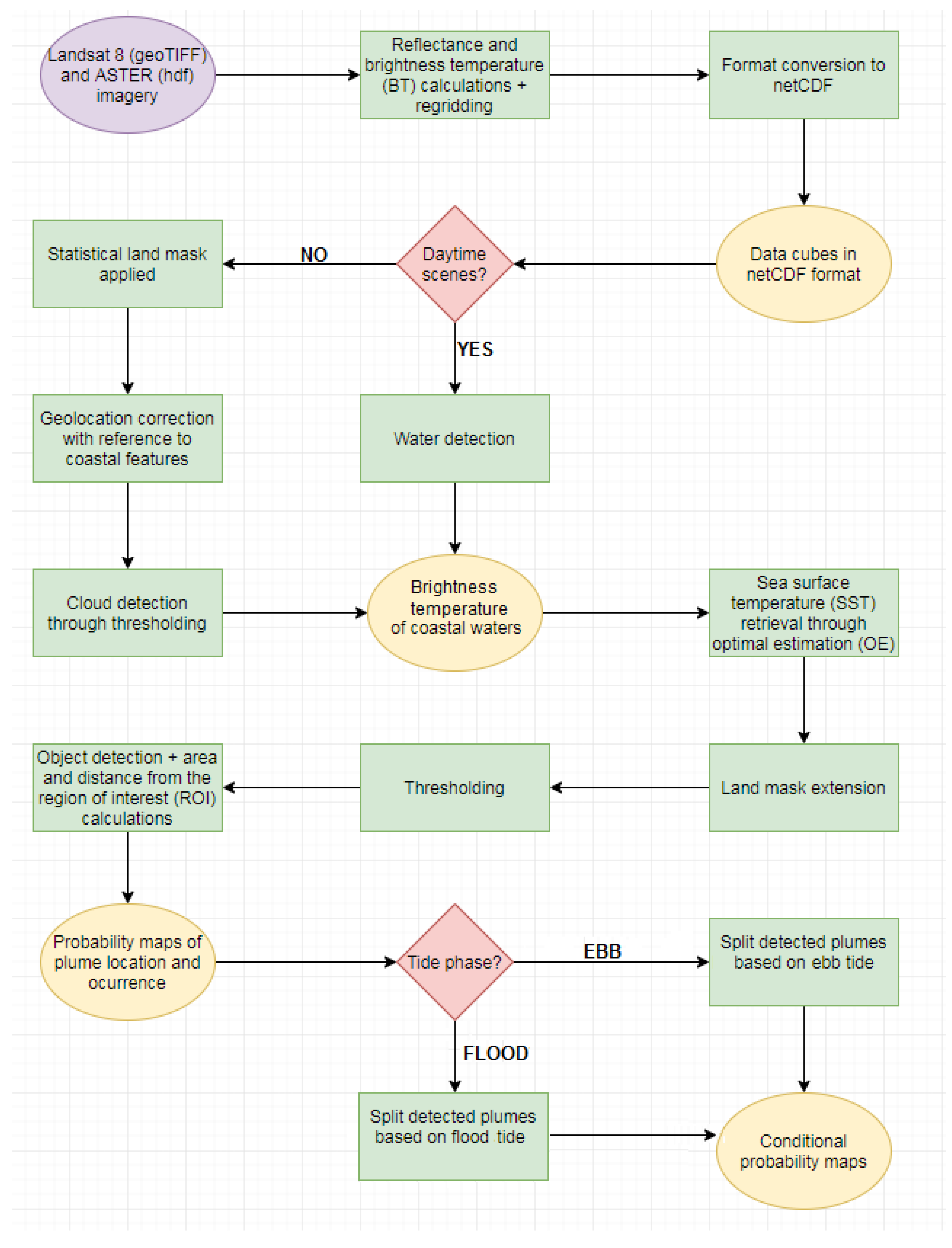
2. Methods
3. Results
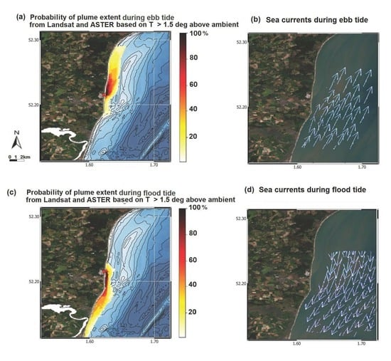
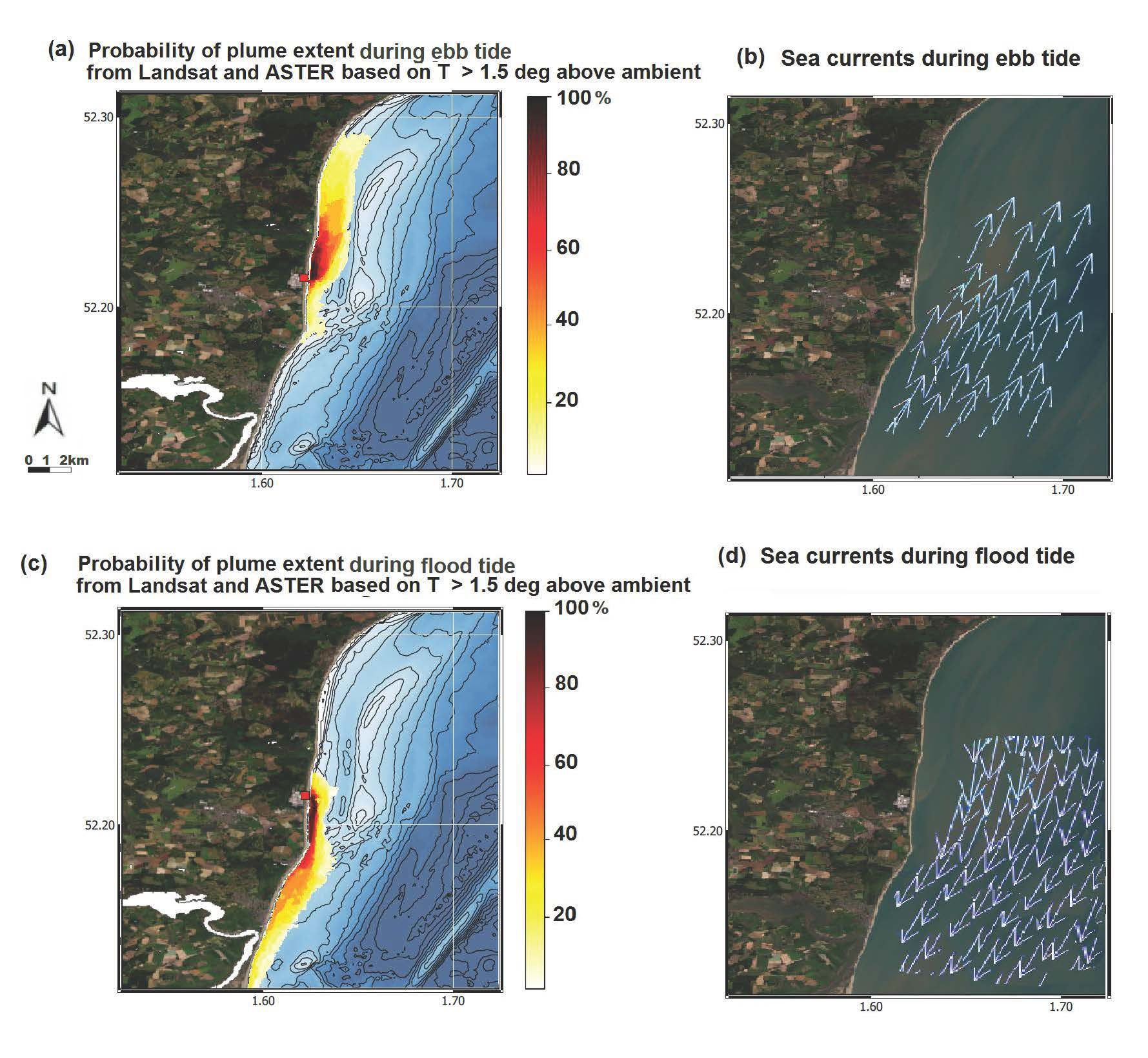
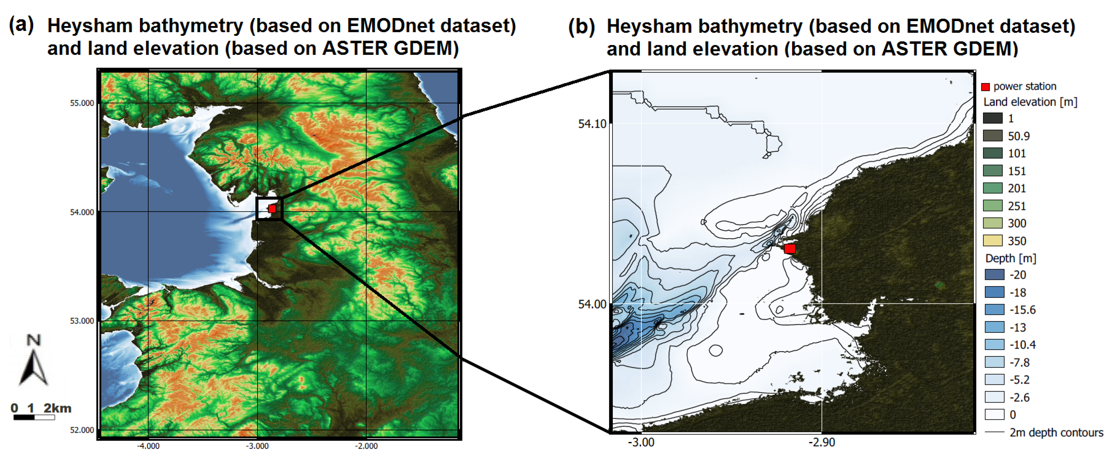
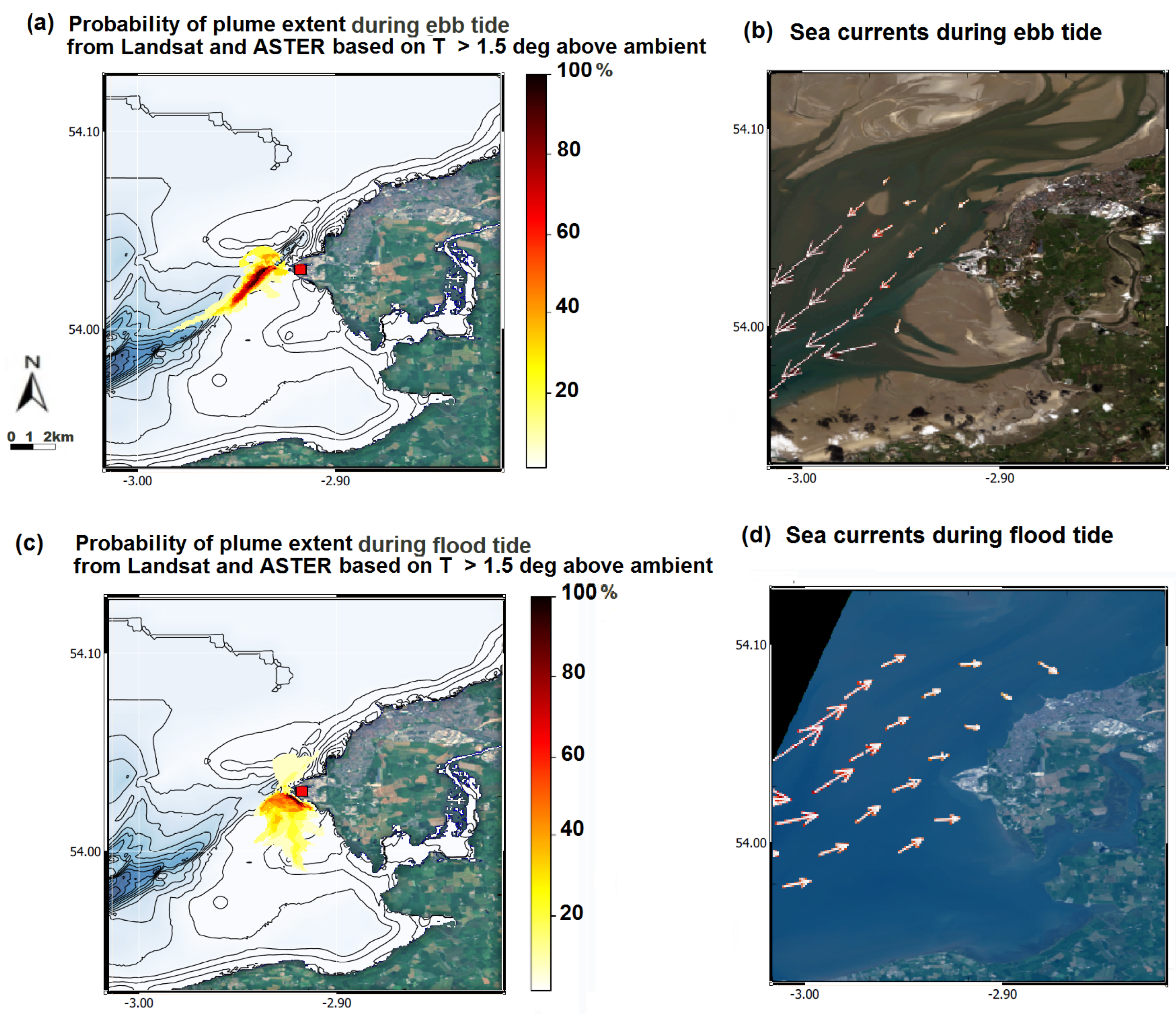
3.1. Heysham as Example of Intertidal Embayment
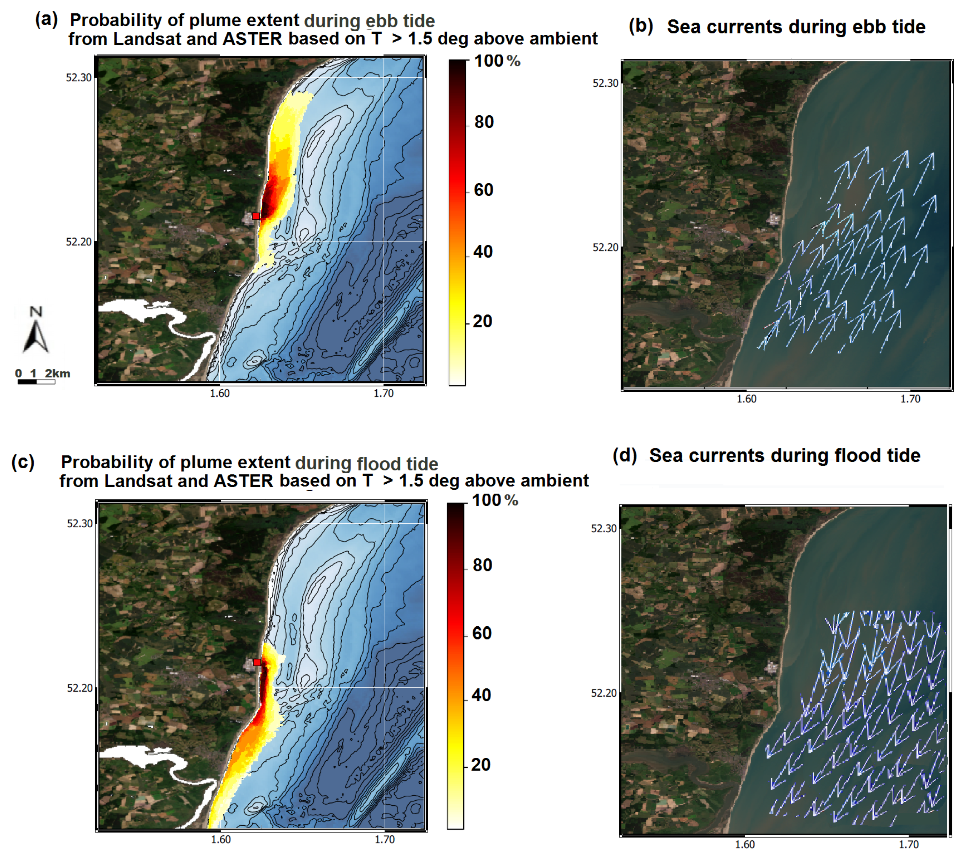
3.2. Sizewell as Example of Open Water Exposure
4. Discussion
5. Conclusions
Author Contributions
Funding
Acknowledgments
Conflicts of Interest
Abbreviations
| ASTER | Advanced Spaceborne Thermal Emission and Reflection Radiometer |
| BEEMS | British Energy Estuarine and Marine Studies |
| BT | brightness temperature |
| CCI | Climate Change Initiative |
| ECMWF | European Centre for Medium-Range Weather Forecasts |
| EMODnet | European Marine Observation and Data Network |
| ESA | European Space Agency |
| GDEM | Global Digital Elevation model |
| MET Norway | Norwegian Meteorological Institute |
| METI | Ministry of Economy, Trade and Industry in Japan |
| MNDWI | Modified Normalised Water Difference Index |
| NASA | National Aeronautics and Space Administration |
| NDWI | Normalised Difference Water Index |
| near-IR | near infrared |
| netCDF | Network Common Data Format |
| NTNG | National Tide Gauge Network |
| NWP | Numerical Weather Prediction |
| OE | Optimal Estimation |
| OLI | Operational Land Imager |
| RGB | red green blue |
| ROI | region of interest |
| RTM | Radiative Transfer Model |
| RTTOV | Radiative Transfer for TOVS (model) |
| SST | sea surface temperature |
| SWIR | short-wave infrared |
| TIR | thermal infrared |
| TIRS | Thermal Infrared Sensor |
| USGS | United States Geological Survey |
| VNIR | visible and near infrared |
References
- Islam, M.A.; Mitra, D.; Dewan, A.; Akhter, S.H. Coastal multi-hazard vulnerability assessment along the Ganges deltaic coast of Bangladesh—A geospatial approach. Ocean. Coast. Manag. 2016, 127, 1–15. [Google Scholar]
- Peponi, A.; Morgado, P.; Trindade, J. Combining Artificial Neural Networks and GIS Fundamentals for Coastal Erosion Prediction Modeling. Sustainability 2019, 11, 975. [Google Scholar] [CrossRef]
- Harik, G.; Alameddine, I.; Maroun, R.; Rachid, G.; Bruschi, D.; Garcia, D.A.; El-Fadel, M. Implications of adopting a biodiversity-based vulnerability index versus a shoreline environmental sensitivity index on management and policy planning along coastal areas. J. Environ. Manag. 2017, 187, 187–200. [Google Scholar] [CrossRef] [PubMed]
- Mei, C.C.; Liu, P. Surface waves and coastal dynamics. Annu. Rev. Fluid Mech. 1993, 25, 215–240. [Google Scholar] [CrossRef]
- Klevanny, K.; Matveyev, G.; Voltzinger, N. An integrated modelling system for coastal area dynamics. Int. J. Numer. Methods Fluids 1994, 19, 181–206. [Google Scholar] [CrossRef]
- De Vriend, H.J. Mathematical modelling and large-scale coastal behaviour: Part 1: physical processes. J. Hydraul. Res. 1991, 29, 727–740. [Google Scholar] [CrossRef]
- Dalrymple, R.A.; Rogers, B. Numerical modeling of water waves with the SPH method. Coast. Eng. 2006, 53, 141–147. [Google Scholar]
- Durán-Colmenares, A.; Barrios-Piña, H.; Ramírez-León, H. Numerical modeling of water thermal plumes emitted by thermal power plants. Water 2016, 8, 482. [Google Scholar] [CrossRef]
- Alesheikh, A.A.; Ghorbanali, A.; Nouri, N. Coastline change detection using remote sensing. Int. J. Environ. Sci. Technol. 2007, 4, 61–66. [Google Scholar] [CrossRef]
- Paduan, J.D.; Rosenfeld, L.K. Remotely sensed surface currents in Monterey Bay from shore-based HF radar (Coastal Ocean Dynamics Application Radar). J. Geophys. Res. Ocean. 1996, 101, 20669–20686. [Google Scholar] [CrossRef]
- Dabuleviciene, T.; Kozlov, I.; Vaiciute, D.; Dailidiene, I. Remote Sensing of Coastal Upwelling in the South-Eastern Baltic Sea: Statistical Properties and Implications for the Coastal Environment. Remote Sens. 2018, 10, 1752. [Google Scholar] [CrossRef]
- Abascal Zorrilla, N.; Vantrepotte, V.; Gensac, E.; Huybrechts, N.; Gardel, A. The Advantages of Landsat 8-OLI-Derived Suspended Particulate Matter Maps for Monitoring the Subtidal Extension of Amazonian Coastal Mud Banks (French Guiana). Remote Sens. 2018, 10, 1733. [Google Scholar] [CrossRef]
- Huang, S.J.; Lin, J.T.; Lo, Y.T.; Kuo, N.J.; Ho, C.R. The Coastal Sea Surface Temperature Changes Near the Nuclear Power Plants of Northern Taiwan Observed from Satellite Images. In Proceedings of the OCEANS 2014-TAIPEI, Taipei, Taiwan, 7–10 April 2014; pp. 1–5. [Google Scholar]
- Muthulakshmi, A.; Natesan, U.; Ferrer, V.A.; Deepthi, K.; Venugopalan, V.; Narasimhan, S. A novel technique to monitor thermal discharges using thermal infrared imaging. Environ. Sci. Process. Impacts 2013, 15, 1729–1734. [Google Scholar] [CrossRef] [PubMed]
- Dai, X.; Guo, Z.; Chen, Y.; Ma, P.; Chen, C. Monitoring of Thermal Plume Discharged from Thermal and Nuclear Power Plants in Eastern China Using Satellite Images. In Proceedings of the 2016 IEEE International Geoscience and Remote Sensing Symposium (IGARSS), Beijing, China, 10–15 July 2016; pp. 7659–7662. [Google Scholar]
- Ma, P.; Dai, X.; Guo, Z.; Wei, C.; Ma, W. Detection of thermal pollution from power plants on China’s eastern coast using remote sensing data. Stoch. Environ. Res. Risk Assess. 2017, 31, 1957–1975. [Google Scholar] [CrossRef]
- Tang, D.; Kester, D.R.; Wang, Z.; Lian, J.; Kawamura, H. AVHRR satellite remote sensing and shipboard measurements of the thermal plume from the Daya Bay, nuclear power station, China. Remote Sens. Environ. 2003, 84, 506–515. [Google Scholar]
- Ahn, Y.H.; Shanmugam, P.; Lee, J.H.; Kang, Y.Q. Application of satellite infrared data for mapping of thermal plume contamination in coastal ecosystem of Korea. Mar. Environ. Res. 2006, 61, 186–201. [Google Scholar] [CrossRef]
- Xu, J.; Zhu, L.; Jiang, J.; Li, J.; Zhao, S.; Yuan, L. Monitoring thermal discharge in Daya Bay plant based on thermal infrared band of HJ-1B and TM remote sensing data. China Environ. Sci. 2014, 34, 1181–1186. [Google Scholar]
- Anupkumar, B.; Rao, T.; Venugopalan, V.; Narasimhan, S. Thermal mapping in the Kalpakkam Coast (Bay of Bengal) in the vicinity of Madras atomic power station. Int. J. Environ. Stud. 2005, 62, 473–485. [Google Scholar] [CrossRef]
- Zoran, M. Nuclear Power Plant’s Water Thermal Plume Assessment by Satellite Remote Sensing Data. In Proceedings of the Global Conference on Global Warming, Lisbon, Portugal, 11–14 July 2011; pp. 11–14. [Google Scholar]
- Xu, H. Modification of normalised difference water index (NDWI) to enhance open water features in remotely sensed imagery. Int. J. Remote Sens. 2006, 27, 3025–3033. [Google Scholar] [CrossRef]
- McFeeters, S.K. The use of the Normalized Difference Water Index (NDWI) in the delineation of open water features. Int. J. Remote Sens. 1996, 17, 1425–1432. [Google Scholar] [CrossRef]
- Kelly, J.T.; Gontz, A.M. Using GPS-surveyed intertidal zones to determine the validity of shorelines automatically mapped by Landsat water indices. Int. J. Appl. Earth Obs. Geoinf. 2018, 65, 92–104. [Google Scholar] [CrossRef]
- Pardo-Pascual, J.; Sánchez-García, E.; Almonacid-Caballer, J.; Palomar-Vázquez, J.; Priego De Los Santos, E.; Fernández-Sarría, A.; Balaguer-Beser, Á. Assessing the accuracy of automatically extracted shorelines on microtidal beaches from Landsat 7, Landsat 8 and Sentinel-2 Imagery. Remote Sens. 2018, 10, 326. [Google Scholar] [CrossRef]
- Merchant, C.; Le Borgne, P.; Marsouin, A.; Roquet, H. Optimal estimation of sea surface temperature from split-window observations. Remote Sens. Environ. 2008, 112, 2469–2484. [Google Scholar] [CrossRef]
- Merchant, C.J.; Embury, O.; Bulgin, C.E.; Block, T.; Corlett, G.; Good, S.A.; Mittaz, J.; Rayner, N.A.; Berry, D.; Eastwood, S.; et al. Satellite-based time-series of sea surface temperature since 1981 for climate applications. Nat. Sci. Data 2019. In press. [Google Scholar]
- Saunders, R. Coauthors, 2013: RTTOV-11 Science and Validation Report. Available online: https://www.nwpsaf.eu/site/download/documentation/rtm/docs_rttov11/rttov11_svr.pdf (accessed on 29 July 2019).
- Hocking, J.; Rayer, P.; Rundle, D.; Saunders, R.; Matricardi, M.; Geer, A.; Brunel, P.; Vidot, J. RTTOV v11 Users Guide, NWP-SAF Report, Met; Office: Exeter, UK, 2014. [Google Scholar]
- Dee, D.P.; Uppala, S.; Simmons, A.; Berrisford, P.; Poli, P.; Kobayashi, S.; Andrae, U.; Balmaseda, M.; Balsamo, G.; Bauer, d.P.; et al. The ERA-Interim reanalysis: Configuration and performance of the data assimilation system. Q. J. R. Meteorol. Soc. 2011, 137, 553–597. [Google Scholar] [CrossRef]
- Merchant, C.J.; Embury, O.; Roberts-Jones, J.; Fiedler, E.; Bulgin, C.E.; Corlett, G.K.; Good, S.; McLaren, A.; Rayner, N.; Morak-Bozzo, S.; et al. Sea surface temperature datasets for climate applications from Phase 1 of the European Space Agency Climate Change Initiative (SST CCI). Geosci. Data J. 2014, 1, 179–191. [Google Scholar] [CrossRef]
- Gonzalez, R.C.; Woods, R.E. Digital Image Processing; Addison-Wesley: Reading, MA, USA, 1992; Volume 2. [Google Scholar]
- Barsi, J.A.; Markham, B.L.; Montanaro, M.; Gerace, A.; Hook, S.J.; Schott, J.R.; Raqueno, N.G.; Morfitt, R. Landsat-8 TIRS Thermal Radiometric Calibration Status. In Proceedings of the Earth Observing Systems XXII. International Society for Optics and Photonics, San Diego, CA, USA, 6–10 August 2017; Volume 10402, p. 104021G. [Google Scholar]
- Abrams, M.; Hook, S.; Ramachandran, B. ASTER User Handbook; Jet Propulsion Laboratory: Pasadena, CA, USA, 2002; pp. 45–54. [Google Scholar]
- Mason, D.; Scott, T.; Dance, S. Remote sensing of intertidal morphological change in Morecambe Bay, UK, between 1991 and 2007. Estuar. Coast. Shelf Sci. 2010, 87, 487–496. [Google Scholar] [CrossRef]
- Coomber, D.P.M.; Hanson, J.D. Estuaries Management Plans: Coastal Processes and Conservation, Morecambe Bay; University of Glasgow: Glasgow, UK, 1994; p. 79. [Google Scholar]
- Lees, B.J. Observations of tidal and residual currents in the Sizewell–Dunwich area, East Anglia, UK. Dtsch. Hydrogr. Z. 1983, 36, 1–24. [Google Scholar] [CrossRef]
- Pye, K.; Blott, S.J. Coastal processes and morphological change in the Dunwich-Sizewell area, Suffolk, UK. J. Coast. Res. 2006, 22, 453–473. [Google Scholar] [CrossRef]
- Sinha, B.; Pingree, R. The principal lunar semidiurnal tide and its harmonics: baseline solutions for M2 and M4 constituents on the North-West European Continental Shelf. Cont. Shelf Res. 1997, 17, 1321–1365. [Google Scholar] [CrossRef]
- Langford, T. Ecological Effects of Thermal Discharges; Springer Science & Business Media: Boston, MA, USA, 1990. [Google Scholar]
- Estuarine, B.E.; Panel, M.S.E. Thermal Standards for Cooling Water from New Build Nuclear Power Stations; British Energy Estuarine & Marine Studies: Severn Estuary, UK, 2011. Available online: https://infrastructure.planninginspectorate.gov.uk/wp-content/ipc/uploads/projects/\EN010001/EN010001-005198-HPC-NNBPEA-XX-000-RET-000212%201.pdf (accessed on 29 July 2019).
- Davies, A.; Sauvel, J.; Evans, J. Computing near coastal tidal dynamics from observations and a numerical model. Cont. Shelf Res. 1985, 4, 341–366. [Google Scholar] [CrossRef]
- Carniello, L.; Silvestri, S.; Marani, M.; D’Alpaos, A.; Volpe, V.; Defina, A. Sediment dynamics in shallow tidal basins: In situ observations, satellite retrievals, and numerical modeling in the Venice Lagoon. J. Geophys. Res. Earth Surf. 2014, 119, 802–815. [Google Scholar] [CrossRef]


© 2019 by the authors. Licensee MDPI, Basel, Switzerland. This article is an open access article distributed under the terms and conditions of the Creative Commons Attribution (CC BY) license (http://creativecommons.org/licenses/by/4.0/).
Share and Cite
Faulkner, A.; Bulgin, C.E.; Merchant, C.J. Coastal Tidal Effects on Industrial Thermal Plumes in Satellite Imagery. Remote Sens. 2019, 11, 2132. https://doi.org/10.3390/rs11182132
Faulkner A, Bulgin CE, Merchant CJ. Coastal Tidal Effects on Industrial Thermal Plumes in Satellite Imagery. Remote Sensing. 2019; 11(18):2132. https://doi.org/10.3390/rs11182132
Chicago/Turabian StyleFaulkner, Agnieszka, Claire E. Bulgin, and Christopher J. Merchant. 2019. "Coastal Tidal Effects on Industrial Thermal Plumes in Satellite Imagery" Remote Sensing 11, no. 18: 2132. https://doi.org/10.3390/rs11182132
APA StyleFaulkner, A., Bulgin, C. E., & Merchant, C. J. (2019). Coastal Tidal Effects on Industrial Thermal Plumes in Satellite Imagery. Remote Sensing, 11(18), 2132. https://doi.org/10.3390/rs11182132