Abstract
This paper presents an algorithm for simulating tomographic synthetic aperture radar (SAR) data based on another stack actually gathered by a real acquisition system. Through the procedure here proposed, the simulated system can be evaluated according to its capability to image complex natural media rather than reference point targets. This feature is particularly important whenever the biophysical properties of the target of interest must be preserved and cannot be easily modeled. The system to be simulated may be different from the original one concerning resolution, off-nadir angles, bandwidth and central frequency. The algorithm here proposed handles these differences by properly taking into account the wavenumbers of the target illuminated by the real survey and requested by the simulated one. The complex images constituting the synthetic stack are associated with the effective vertical interferometric wavenumber peculiar of the geometry to be simulated, regardless of the original data. Furthermore, the three-dimensional resolution cell of the simulated tomographic system is consistent with the simulated geometry concerning size and spatial orientation. These two latter features cannot be guaranteed by simply filtering the original stack. The simulator here proposed has been used to simulate the tomographic stack expected from the forthcoming European Space Agency (ESA) BIOMASS mission. The relationship between baseline distribution and 3D focusing capability was explored; special attention has been paid to the robustness of tomographic power at being a good proxy for the above ground biomass in tropical regions.
1. Introduction
The design of any spaceborne synthetic aperture radar (SAR) mission poses several challenges, among others the definition of the orbital path or the amount of propellent on board. The vast majority of the system parameters cannot be adjusted after the launch, so their tuning cannot take advantage of the feedback provided by the first acquisitions. This issue, together with the great investment of resources, drives the attention on the reduction of hazards, namely on derisking. Usually, both technological choices and image formation can be properly modeled or simulated. End-to-end descriptions of the acquisition system are developed and can provide the expected output given any input target. Recently, several algorithms have been recently developed for this purpose. Efforts have been made to reduce the computational burden of the simulator especially whenever non-straight orbits are considered [1,2].The electromagnetic features of the structures to be simulated have been studied too, geometrical optics, physical optics and full wave approaches have been proposed [3,4]. Furthermore, ground topography and interferometric processing have been explored [3,5]. These approaches are particularly effective whenever the reference targets are simple (their response is almost known) and the processing chain, up to parameters retrieval, is consolidated. These two conditions are not met in the case of complex natural media and tomographic [6,7] measurements. Targets such as snowpacks [8], glaciers [9] and unmanaged forests [10,11,12] are currently under investigation and any model takes the risk of masking meaningful features. In particular, the analysis of dense forests is the main driver of the forthcoming ESA BIOMASS mission [13] whose launch is expected in 2022. The penetration capability of its P-band signal is expected to provide an insight of many environments as deserts and glaciers in addition to any forests (refer to [14] for further details). Acquisitions on vegetated areas, most importantly on tropical regions, will be processed to generate a map of Above Ground Biomass (AGB) at global scale. Tropical forests are very hard to reduce to a small number of significant elements, moreover the relationship between AGB and radar backscatter is not yet fully understood [15,16]. As a consequence, assessing the impact of any change in BIOMASS system parameters on its capability to retrieve the AGB amount is not trivial and requires a specific strategy. The method here proposed relies on the exploitation of real tomographic SAR images gathered on forests by airborne systems for obtaining a description of the scene; this latter being recovered by means of the back-projection [17] algorithm. Then, the 3D reconstruction of the forest is projected into a tomographic stack in accordance with the geometry of acquisition and radar parameters of the spaceborne system to be simulated. This simple approach requires special care due to the different wavenumbers that gave rise to the airborne radar echo and that are illuminated by the simulated spaceborne system. Also, the three dimensional resolution cells of the two tomographic systems differ as regards their size (dependent on the bandwidth) but also their orientation because of the different acquisition geometry. This latter issue in particular cannot be accounted for by simply filtering the real airborne data stack.
The simulator here proposed has been used to estimate the spaceborne tomographic reconstruction provided by the BIOMASS system. Particular attention has been paid to the power fluctuations due to inaccurate orbital control, that is to irregular baseline sampling. This fluctuations impact on the capability of the BIOMASS system of producing measurements to be used as proxy for AGB estimates. The deterioration of the correlation with AGB of tomographic derived quantities could be observed as a function of orbital inaccuracies.
This paper is organized as follows: in Section 2 a short description of tomographic SAR imaging in the wavenumber domain is presented, highlighting the differences between airborne and spaceborne systems; in Section 3 the procedure for simulating tomographic stacks starting from real acquisitions is detailed (The simulation strategy described in this paper was used to simulate BIOMASS data on boreal and tropical forests that were delivered to European Space Agency (ESA) as a part of the SARSIM database [18]); Section 4 illustrates some features of the synthetic tomographic stack; Section 5 presents the analysis of the impact of orbital inaccuracies on AGB estimates; in Section 6 conclusions are drawn.
2. Wavenumbers in SAR Acquisitions
This section recalls the basic principles of any SAR surveys. The transmitted signal, the scene under observation and their interaction are described in two conjugated domains. The former is the direct domain, that is time or space; the latter is the frequency domain, usually referred to as wavenumber domain when spatial coordinates are transformed. This representation is particularly useful due to the possibility of interpreting SAR acquisitions in terms of enlightenment of the target’s components. Also, the simulation procedure, core of this work, can only be described by resorting to this approach.
The change of domain is achieved by computing the Fourier transform [19] of the function of interest, that is projecting it on a set of complex exponentials of the form shown by Equations (1) and (2) for signals defined over time and spatial maps respectively.
The basis function expressed by Equation (2) has unitary magnitude and phase varying along a specific direction only. This direction is defined by the direction of the real vector ; by moving on the plane perpendicular to no changes occur. For this reason, vector is referred to as wavevector, its components , and are known as wavenumbers. The speed of the phase rotation is determined by the magnitude instead: the longer the faster the oscillations. Due to the orthogonality of two complex exponentials having different wavevectors, the function in Equation (2) defines a point in the domain, that is the wavenumber or the spatial frequency domain. Signals traveling in both space and time can be described either in the frequency domain or in the wavenumber domain by freezing time or by focusing on a specific spatial coordinate; the relationship between the propagation in time and in space is ruled by the propagation speed, the speed of light in vacuum c is assumed throughout all this discussion.
The transmitted radar pulse can be described in the temporal frequency domain through a function defined on a limited spectral support: it is centered on the carrier frequency and width is given by the bandwidth B. In the far field approximation, this very same signal can be described in the spatial domain as a plane wave. According to this approximation, the direction of propagation, that is the direction of the wavevector , is defined by the line joining the sensor and the point (P in Figure 1) far away where the signal is evaluated. The extended bandwidth implies the existence of many waves of the form expressed by Equation (1), each one oscillating at a different frequency. Then, the corresponding spectral support in the wavenumber domain is a line directed as , with length proportional to the system bandwidth and distance from the origin linked to the carrier frequency. It follows that the link between temporal and spatial frequencies depends on the geometry of acquisition, in particular on the look angle (or off-nadir angle) specified by in Figure 1.
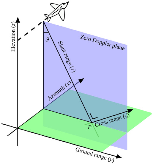
Figure 1.
Schematic representation of a zero squint synthetic aperture radar (SAR) acquisition. The off-nadir angle (also known as look angle) defines the line-of-sight and hence the cross range axis ; both of them lying in the zero-Doppler plane, orthogonal to azimuth. The cross range (proportional to the elevation) is a blind direction for single-image SAR systems: sensitivity to the direction is provided by interferometric or tomographic SAR systems.
The interaction between wave and target generates a set of waves scattered in all directions. In this discussion only the waves traveling back to the radar are considered, that is, only the monostatic case is analyzed. The two-way travel path implies that the wavenumbers of the target responsible for the backscattered echo are twice the ones of the signal impinging on the target itself [20]. Then, the spectral components giving rise to the radar echo, lie on a line centered on and with length ; these latter quantities are defined by Equations (3) and (4).
The dashed line in Figure 2 is an example of the spectral components illuminated in a highly localized target by a radar in fixed position. The length of this line is connected to the resolution that the radar system can provide along the line-of-sight. The capability of resolving target along the azimuth direction typical of SAR systems can also be interpreted in terms of wavenumbers. A set of acquisitions gathered along the platform trajectory are characterized by spectral lines whose distance from the origin and length are constant (as they depend on radar parameters) but change orientation (being the same as the line-of-sight). The spectral region illuminated by a SAR survey is shown in Figure 2 as a grey surface. The extension of this patch is linked to the resolution that the SAR system can provide; the 2D extent of this surface reflects the lack of resolution of SAR systems along the direction orthogonal to the line-of-sight and to azimuth. That is, standard SAR systems cannot resolve targets lying along the cross range direction depicted in Figure 1.
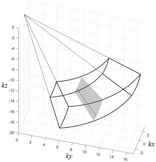
Figure 2.
Geometrical loci associated with the wavenumbers illuminated by a typical airborne SAR system. A small target, observed from a fixed azimuth position, is associated with the dashed segment here shown: the distance from the origin being proportional to the radar central frequency, its length to the system bandwidth and its orientation following the segment connecting sensor and target (the local line-of-sight). The set of segments associated with every position of the sensor within the synthetic aperture is shown as a gray surface. The set of patches associated with all the off-nadir angle explored by the physical antenna gives rise to the volume whose edges are shown as thick lines.
The grey surface in Figure 2 is the spectral enlightenment associated with a single (or a narrow range) look angle ; the corresponding surface for a look angle can be obtained by rotating this patch around the axis by an angle .
The set of all these surfaces defines a volume in the domain, its edges are shown as thick lines in Figure 2. The spectral spread along the cross range direction should not suggest the possibility of resolving targets in the 3D space though. As a matter of fact, this spectral spread only exists if different parts of the scene are considered together, it disappears for a single target. The very same feature can be appreciated by analyzing the spectral enlightenment along the azimuth direction; in order to do this the constraint of local analysis must be relaxed and the waves must be considered as spreading spherically from the radar rather than being plane. For any fixed azimuth position occupied by the sensor, a large spatial region is reached by the transmitted signal, its extension along x depending on the antenna beamwidth. It follows that many wavenumbers along are illuminated at once; however, they are associated with different targets on the ground thus providing a narrow band signal (hence no resolution) for each of them. A wideband signal along can only be produced by combining the echoes gathered by the sensor along its path, that is building a synthetic antenna. Analogously, many images of the same target are needed if resolution along the cross range is desired, each one gathered from a different look angle. This issue is discussed more in detail in the following subsection.
2.1. Wavenumbers in SAR Tomography
For the sake of simplicity, the discussion in this section hypothesizes the absence of a squint angle in the antenna pointing and in the focusing algorithm. Holding this condition, after azimuth compression this direction can be considered as decoupled from the other two. For this reason, the following analyses are carried out considering only the zero Doppler plane shown in Figure 1 rather than the whole three-dimensional space. This plane hosts many targets whose common feature is the position of the center of the synthetic antenna, this point also lies on the zero Doppler plane and it is often synthetically referred to sensor position. Whenever the area is imaged several times, each target can be associated with many sensor positions: a proper acquisition plan and processing steps ensure that every sensor position lies on the zero Doppler plane. One of them shall be chosen as reference sensor in order to define the nominal geometry (range axis, look angle and so on), this favored sensor is referred to as master whereas the others as slaves. The definition of a nominal geometry enables to parametrize the zero Doppler plane by means of a pair of orthonormal unit vectors directed as the line joining master and target (slant range) and cross range as shown in Figure 1. As opposed to a coordinate system, rotates with the range coordinate however it always highlights the directions along which a single SAR image has resolution capabilities (slant range) and where it lacks (cross range).
The vector joining any two sensors is known as baseline, it can be conveniently expressed as a sum of its components along the slant range and cross range; the former is referred to as parallel baseline whereas the latter as normal baseline. The larger the baseline the further the two sensors, however only the normal component is responsible for a change in the look angle associated with the two positions. The existence of a difference in the look angles implies different directions of arrival of the wave when it impinges on the target. This, in turn, leads to different wavenumbers of the same target illuminated by the two sensors. The geometrical locus in the plane associated with the tomographic acquisition is a set of segments [21], each of them with a different tilt; they are shown in Figure 3 in case of regularly spaced normal baselines and for a nominal look angle of . The spread of the spectrum provided by the various acquisitions results in the possibility of resolving targets along the cross range direction as well. The relationship between resolution and spectral width is expressed by Equation (5).
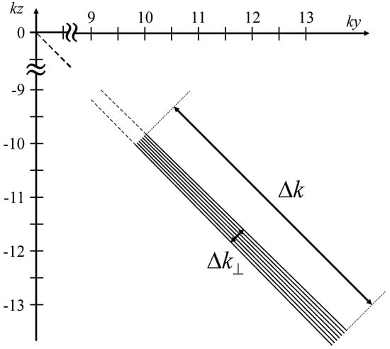
Figure 3.
Geometrical loci associated with the wavenumbers illuminated by a tomographic SAR survey for a single target in the domain; each segment being associated with a different image of the tomographic stack. The spectral extension shown as is proportional to the resolution in the range direction and is not improved by processing several images together. On the contrary, the slightly different off-nadir angle associated with each acquisition provides bandwidth along the perpendicular direction, here shown as . This finite extent is related to the resolution capability of a TomoSAR system along the cross range direction shown in Figure 1.
can be expressed as a function of the central frequency and look angles as shown in Equation (6).
where is the largest difference of look angles. The order of magnitude of can be appreciated by considering a typical P-band tomographic system whose parameters of interest are summarized in Table 1.

Table 1.
Parameters of a typical P-band tomographic system.
By combining Equations (3), (5) and (6) a value of about for results. It must be kept in mind that the wavenumber region whose width is , is sampled in the transformed domain thus leading to a periodic signal in the direct domain in case of regularly spaced baselines. The period in the cross range direction is related to the sampling step according to Equation (7).
where is the separation in the wavenumber domain between subsequent passes, it can be expressed as , N being the total number of passes.
2.2. Wavenumbers in Airborne and Spaceborne SAR Surveys
The much greater distance from sensor to target makes spaceborne SAR surveys rather different from airborne ones. Main differences are due to the significant atmospheric layer through which the signal propagates and to the similarity between near and far range. This section focuses on this latter issue and assumes that the propagation has been properly taken into account thus achieving a good azimuth compression.
Airborne systems usually flight between ∼2 km and ∼10 km of altitude thus resulting in a wide range of look angles within the swath; as a general rule, near range targets are associated with look angles of about reaching in far range, this values being mainly determined by the antenna beamwidth in the elevation direction. On the contrary, the swath width of a spaceborne system shall be set according to the need of avoiding undesired ambiguous echos and nadir returns. These constraints together with the large distances at stake lead to a very small range of look angles; as a rule of thumb, it may change by from near to far range. These features impact on the spectral region illuminated by the two systems in the domain. Figure 4 shows the wavenumbers excited by an airborne system (in green) and a spaceborne one (in purple). With respect to the airborne, the spaceborne system here considered has a higher carrier frequency but a much lower bandwidth. The dashed line in Figure 4 shows the wavenumbers associated with the carrier frequency as the acquisition moves from near to far range. Its distance from the origin is constant and expressed by Equation (3) whereas its rotation depends exclusively on the geometry of acquisition. According to this, a polar system of coordinates turns out to be particularly helpful in this context; the relationship between the two coordinate systems are expressed by Equations (8)–(10).
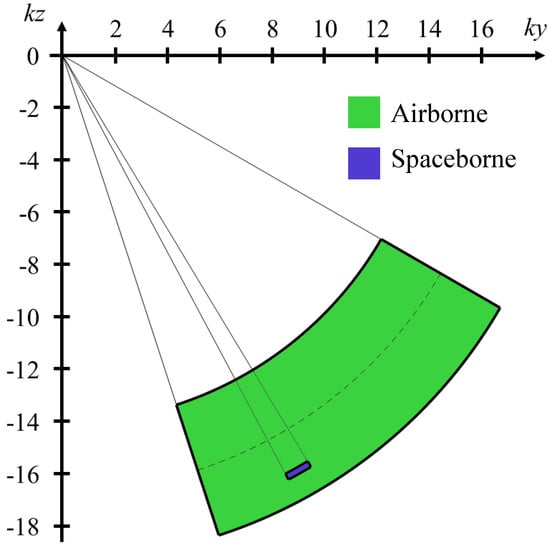
Figure 4.
Wavenumbers enlightened by an airborne (green) and spaceborne SAR systems (purple) in the domain. The horizontal axis represents the transformed variable of the ground range coordinate whereas the vertical axis of the elevation; y and z in Figure 1 respectively. The airborne system here represented spans a wider range of look angles, has a greater bandwidth and a lower central frequency than the spaceborne system.
The wavevectors pointed out by the dashed line in Figure 4 obey to the relationship expressed by Equation (11).
A comparison between the impulse response functions (that is, the point spread functions) of airborne and spaceborne systems is shown in Figure 5 for difference range values.
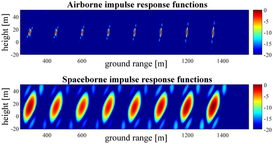
Figure 5.
Impulse response functions (IRFs) in the zero-Doppler plane varying the distance from the radar. The IRFs of the airborne system changes significantly (mainly its rotation) from near to far range whereas the spaceborne system is almost constant. The horizontal and vertical axes refers to the ground range (y) and elevation (z) axes shown in Figure 1 respectively. The height is here referred to a constant elevation taken as a reference.
3. Cross Sensor Simulation
This section illustrates a procedure for the simulation of a tomographic SAR stack starting from another one with possibly different carrier frequency, bandwidth and geometry of acquisition. Quantities associated with the first system will be labeled with a , the second with a ; this follows the practical need of simulating a spaceborne system starting from an airborne one although the algorithm here illustrated can be applied to any systems pair.
The algorithm here presented relies on the exploitation of Equation (12) [22,23,24] for each azimuth position.
where represents the complex reflectivity distribution in the plane, is the waveform envelope, r is the range coordinate and R is the distance between each point scatterer and sensor. Equation (12) models the generation of any range line of a SLC SAR image: the integral expresses the coherent sum of the scattering coefficients associated with targets placed at the same distance from the sensor, the complex exponential describes the demodulation of the target spectrum in accordance with the radar central frequency and the convolution represents the filtering due to the limited signal bandwidth. The knowledge of system parameters and acquisition geometry leads to two unknowns only in Equation (12), they are the scatterers’ distribution and the SAR image . The availability of a stack of SAR images allows SAR tomography to be implemented, through which an estimation of the reflectivity map can be obtained. On the other hand, by feeding Equation (12) with any scatterers’ distribution, a synthetic SAR image can be straightforwardly produced. The generation of a synthetic stack starting from real tomographic data relies on these two steps. Firstly, the reflectivity profile is estimated by performing SAR tomography on real data and then it is used, along with the parameters of the system to be simulated, to produce the synthetic images. However, due to the difference between the two acquisition systems, an extra processing step is needed to make the reconstruction provided by the first compatible with the second.
The complex exponential in Equation (12) is responsible for a demodulation of the spectrum of the target before being filtered by ; as a consequence, only the passband components of contribute to . However the spatial direction along which this demodulation takes place is ruled by the range axis, whose direction changes from near to far range. Or rather, the wavevectors of that contribute to have constant magnitude for each value of r but they change direction in accordance with the look angle. It follows that should lie on the spectral support defined by the acquisition system to be simulated for generating correct range lines. The spectral properties of the target are properly taken into account by the back-projection tomographic algorithm: the reconstructed profile is band-limited and pass-band. However, it lies on the spatial frequencies illuminated by the first system which might be different from the ones required by the second.
The reflectivity map returned by the back-projection algorithm when applied to real data will be referred to as . This function, if fed directly into Equation (12) would lead to incorrect results the more the simulated system is different from the real one. The convolution expressed in Equation (12) amounts to a product in the wavenumber domain between the Fourier transform of the system filter (whose support corresponds to the spectral enlightenment) and the reflectivity spectrum of the target. Then, for an acquisition to be properly simulated, these two spectral regions must overlap for all the range line, that is, for every look angle. The overlap must occur in the plane so the reflectivity spectrum must match the spectral enlightenment concerning both angle and central frequency. Typically, the angular agreement between the two systems is reached for a narrow interval of distances sampled by the airborne system. It follows that feeding directly into Equation (12) would result in SLCs almost completely empty as a consequence of the different spectral support of and the system filter. Moreover, a large discrepancy in the central frequencies (or a relatively small bandwidth) gets the two spectral regions separated regardless of the look angle. In order to guarantee the correspondence of wavenumbers, the estimated reflectivity profile must be spectrally translated around the wavenumbers illuminated by the simulated system; in the remainder of this section, it is illustrated how this translation can be achieved through a spatial demodulation followed by a modulation.
The reflectivity profile at radio-frequency can be taken to baseband (in the domain) by compensating the phases associated with the local distances. The spatial map demodulating the reflectivity profile can be expressed as in (13).
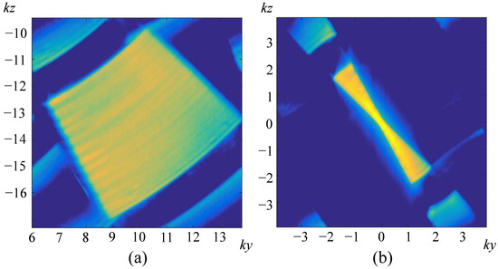
where represents the distance of each pixel of from the master sensor and the central wavelength used by the airborne system. The product between and modifies the spectral support of the reflectivity function and takes it into baseband. Locally, that is for every look angle, it amounts to a translation of the corresponding spectral line along the direction defined by the spectral line itself; however, different look angles are associated with spectral lines with different orientations so that the translation always follows the radial direction. As a consequence, the shape of the spectral support of is modified: from a section of a ring to a “butterfly” shaped region as shown in Figure 6. The thickness of the butterfly around the origin in the direction orthogonal to the line-of-sight is connected to the resolution of the reflectivity map along the cross-range direction that the airborne system is able to provide. Real spectra before and after the spatial demodulation are shown in Figure 7. The reflectivity profile can be taken in the surrounding of the wavenumbers illuminated by the spaceborne system by another modulation; the modulating map is shown in Equation (14).
where represents the distance of each pixel of from the master sensor of the spaceborne system to be simulated and its central wavelength. The generation of the reflectivity map whose spectral support is suited for the projection into a stack of spaceborne images, is shown in Equation (15).
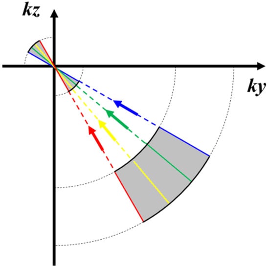
Figure 6.
Demodulation of the reflectivity map depicted in the domain. The multiplication by the function defined in Equation (13) takes every spectral line into baseband along the direction defined by the local line-of-sight.
can be fed into Equation (12) to generate the tomographic stack of the system to be simulated. This latter can be explored with the back-projection tomographic algorithm and the 3D reconstruction compared with the corresponding airborne; this comparison is shown in Figure 8.
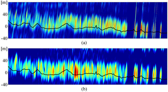
Figure 8.
Tomographic profiles returned by the back-projection algorithms when applied to (a) real airborne data and (b) simulated spaceborne stack. The two axes are analogous to the ones shown in Figure 5; the black line shows the ground topography below the forest layer estimated through SAR tomography [25].
4. Features of the Simulated Stack
The correct interpretation of the simulated stack of images is not trivial; some features can be understood by exploring the processing chain outlined in Section 3. Again, the real system will be referred to as “airborne” whereas the simulated one as “spaceborne” although this layout is not mandatory. Also, this paragraph focuses on the impact of the distribution only rather than both and due to the 1D nature of the issues here raised.
In general, the tomographic airborne system makes available some wavenumbers of the target whereas the spaceborne system requests others. Each image of the airborne system samples a specific so that a sampled version of the Fourier transform of the vertical reflectivity profile of the target is collected. It follows that the reconstruction of the reflectivity profile, obtained for example through back-projection, is periodic. This periodicity implies that its Fourier transform exists exclusively in correspondence of the original values, it goes to zero for every other value. Should the spaceborne system require a new then some expedient is needed. A possible solution amounts to interpolating the signal in correspondence of the desired value; this, in turn, corresponds to windowing the reconstructed reflectivity profile lying in the z domain. It follows that the reflectivity profile may be reconstructed for a limited range of elevations avoiding the replicas. This precaution saves computational time when computing the back-projection and, at the same time, allows the generation of SLC images in correspondence of new values. The generation of data in correspondence of very large values (outside from the sampled range) is possible only through extrapolation and hence it should be avoided as it amounts to fabricating details.
The aforementioned concepts are strictly valid for regular spatial sampling only; highly irregular sampling of the axis in the airborne leads to artifacts in the simulated SLCs. Windowing the reflectivity profile amounts to a convolution between the signal and the kernel of the window, for instance a sinc. Should two subsequent sampled be too far away, then the interpolated signal in the middle will be weaker; that is, the synthetic SLC corresponding to a far from the sampled ones will be less powerful. Also, due to the high variability of the distribution in airborne surveys this power loss is dependent on the spatial coordinate. The synthetic SLCs may exhibit power fluctuations due to the space varying sampling of the axis. However, the tomographic profile estimated with the synthetic images is consistent with the one resulting from the original one up to resolution losses. Instability in the distribution of the airborne survey leads to fluctuations in the interferometric phase, in the simulated spaceborne stack this latter is exchanged for amplitude fluctuations of the SLC images. This effect is shown in Figure 9.
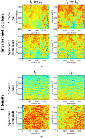
Figure 9.
As discussed in Section 4, platform deviations lead to fluctuations in the interferometric phase. The straight orbits of the (simulated) spaceborne system removes phase fluctuations by exchanging them for power oscillations.
It must be observed that the simulated stack is not affected by the propagation of the signal more than the real stack is. For a spaceborne simulation to be more realistic the effects of the propagation of the wave through troposphere and ionosphere should be included. However, phase screens may be straightforwardly added to the simulated SLC images; for a even more faithful simulation, they can be defocused and the atmospheric contribution applied to the synthetic raw images.
A final comment on the physical phenomena giving rise to the radar echo is in order. The target features responsible for the backscattered power change with the central frequency of the signal; for instance, shorter waves experience a stronger attenuation and are influenced by smaller structures. The possibility of “changing” the central frequency offered by the algorithm here proposed does not imply the exploration at another scale of the target. The radiometric properties together with the polarimetric signature are determined by the real dataset. The signal gathered at a certain frequency is simply mapped to another. The response of the target when observed at a certain frequency does not provide any indication of its interaction with a signal with different wavelength unless explicitly postulated by certain physical model.
5. Application to BIOMASS: Impact of Orbital Control
The concepts illustrated in the previous sections have been used to simulate the spaceborne tomography that is expected from the ESA BIOMASS mission [13]. The effect of non regularly spaced orbital paths was explored; in particular, their impact on the estimated tomographic power and its correlation to the Above Ground Biomass (AGB). The real airborne stack providing the input have been gathered by ONERA in 2009 over the Paracou area in French Guiana in the context of the TropiSAR campaign [26]; the phases of this image stack were further calibrated according to the procedure described in Reference [27]. The parameters of interest of both systems are listed in Table 2; the scene has been cropped to include only the ROIs with the ground truth measurements of the AGB. The azimuth resolution of the spaceborne system was set to m by means of a simple low-pass filtering. A description of the site providing the ground truth measurements can be found in Reference [28] and references therein whereas the estimation of the above ground biomass is detailed in Reference [29].
Table 2.
Parameters of the P-band airborne radar used in the ONERA TropiSAR survey over Paracou and simulated spaceborne system.
The baseline distribution of the BIOMASS system is designed to span the of the critical baseline with 7 subsequent passes regularly spaced, resulting in a vertical resolution of about 20 m. Any orbital drift changes the spatial sampling of the total baseline aperture which, in turn, modifies the vertical Impulse Response Function (IRF) of the tomographic system. The vertical IRF determines the effectiveness of the system in focusing on a specific elevation and rejecting the surrounding echoes. Then, it is expected that any deviations from the nominal orbits perturb the correlation between tomographic power and AGB [15]. In order to evaluate this perturbation the spaceborne system has been simulated several times, each time with slightly different orbital paths. Then, the spaceborne tomography has been generated and the resulting power was put in relation with AGB.
The displacement of each sensor from its nominal position was simulated by means of a Guassian random variable. The displacements involve only the longitude of the orbits, being kept constant the elevation above the Earth’s surface. Also, the total baseline aperture was kept constant and equal to the nominal one, only the five innermost tracks were perturbed. Their fluctuations were modeled by a zero average Gaussian random variable whose standard deviation was increased from to of the critical baseline; for each value of this standard deviation 10 outcomes were generated.
Figure 10 shows the nominal positions of the sensors together with the outcomes; each panel refers to a different perturbation strength. The corresponding vertical IRF is shown in Figure 11; the horizontal axis refers to the elevation whereas the vertical represents the attenuation in dB, the vertical bars refer to . It may be observed that driving away from the regular sampling leads to smaller rejection of the echoes coming from surrounding elevations and a larger uncertainty in the exact dB value.
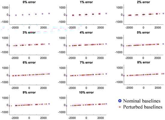
Figure 10.
Sensor positions in the zero Doppler plane of the simulated spaceborne system; regularly spaced (nominal) positions are shown as blue circles, irregular positions as red asterisks. The irregular coordinates have been obtained by modifying the nominal positions with a Gaussian perturbation, the elevation above the Earth surface being kept constant. The amount of perturbation is defined by the standard deviation of the Gaussian noise as a percentage of the total baseline aperture. In this work, 11 perturbations have been tested from to . The corresponding sampling of the total baseline aperture is shown in the 11 panels here shown.
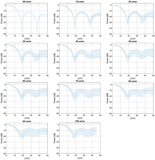
Figure 11.
Tomographic SAR systems offer the possibility of focusing on specific depths by attenuating the radar echoes coming from surrounding elevations; the vertical discrimination can be appreciated by analyzing the impulse response functions (IRFs) here shown. The elevation of interest is here set around 0 m (with respect to a given reference height) that is, where the IRFs reach the maximum value. The attenuation of the echoes coming from other elevations is shown in dB in the vertical axis, being the horizontal axis the distance from the desired elevation in meters. Irregularities in the baseline distribution modify the IRF and worsen the capability of the tomographic system of rejecting undesired radar echoes. The panels here shown correspond to the sensor positions shown in Figure 10. 10 outcomes of the Gaussian noise perturbing the baselines have been generated for each perturbation intensity (going from to of the critical baseline); the average IRF, together with the errorbars are here shown.
For each outcome of the sensors positions, the tomographic power coming from 40 m above the ground level was estimated and then put in relation with AGB. The choice of 40 m rather than 30 m [15] was driven by the need to take the ground level in correspondence of a zero of the vertical impulse response function (see Figure 11) as suggested in Reference [30]. Many scatterplots as shown by the top panel of Figure 12 were computed and for each one the linear fit estimated. The effectiveness of the tomographic power at being a good proxy for AGB has been assessed by evaluating the correlation coefficient and the sensitivity to AGB; this latter expressed in dB/(Mg/Ha·100) so that a high value suggests more robust estimations. The behavior of the correlation and the sensitivity varying the orbital irregularities is shown in the bottom panels of Figure 12; again, the error bars express . As expected, the correlation between tomographic power and AGB drops by moving toward an irregular configuration, at the same time the dispersion around the average value increases. The same happens for the sensitivity, reaching a plateau after an error of about of the critical baseline.
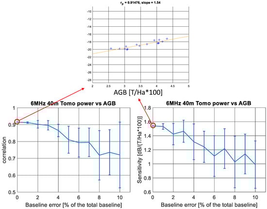
Figure 12.
Evolution of the sensitivity and correlation to the above ground biomass (AGB) of the tomographic power at 40 m above the ground level as the sampling of the baseline aperture drives away from the regular grid. The top panel shows the scatterplot relating tomographic power and AGB in case of perfectly regular sampling.
6. Conclusions
In this paper, a new procedure for simulating a tomographic SAR stack was presented; the main free parameters of the system to be simulated are: sensors positions, central frequency and bandwidth. The target of interest comes from tomographic reconstruction based on actual data acquired by a real SAR system. The possibility of simulating SAR images based on real data is particularly convenient whenever the scene is complex and all physical phenomena must be respected rather than modeled. The two systems may be tuned on different central frequencies, have different bandwidths, cover different look angles and provide different vertical resolutions. Special attention was paid to account for all these differences resulting in a simple yet effective procedure. The algorithm here proposed relies on the identification of the spatial frequencies of the target made available by the real system and required by the simulated one. This analysis was made possible by interpreting SAR tomography in the wavenumber domain. The procedure here proposed allows for the desired geometry of acquisition to be properly simulated, in terms of both distribution and shape of the three-dimensional resolution cell. It must be observed that these properties cannot be imposed through a simple filtering of the original stack. The features of the resulting stack were discussed as well; in particular, it was shown that each image of simulated stack may be characterized by power fluctuations depending on the instability of the platform providing the original stack.
The simulator here proposed was implemented and used to simulate the tomographic stack that will be provided by the forthcoming ESA BIOMASS mission; the input data coming from the TropiSAR airborne campaign. It was possible to evaluate the relationship between tomographic power and above ground biomass as a function of the baselines irregularities.
Author Contributions
Conceptualization, M.M.d. and S.T.; Methodology, M.M.d. and S.T.; Software, M.M.d. and S.T.; Validation, M.M.d. and S.T.; Formal Analysis, M.M.d. and S.T.; Investigation, M.M.d. and S.T.; Resources, S.T.; Data Curation, M.M.d.; Writing—Original Draft Preparation, M.M.d.; Writing—Review & Editing, M.M.d. and S.T.; Visualization, M.M.d.; Supervision, M.M.d. and S.T.; Project Administration, S.T.; Funding Acquisition, S.T.
Funding
This research received no external funding.
Acknowledgments
The authors wish to acknowledge the European Space Agency and the whole Level-2 team of the ESA BIOMASS mission for providing the framework in which this algorithm was developed.
Conflicts of Interest
The authors declare no conflict of interest.
Abbreviations
The following abbreviations are used in this manuscript:
| AGB | Above ground biomass |
| DBH | Diameter breast height |
| IRF | Impulse response function |
| SAR | Synthetic aperture radar |
| SLC | Single look complex |
| TomoSAR | Tomographic SAR |
References
- Franceschetti, G.; Iodice, A.; Perna, S.; Riccio, D. SAR Sensor Trajectory Deviations: Fourier Domain Formulation and Extended Scene Simulation of Raw Signal. IEEE Trans. Geosci. Remote. Sens. 2006, 44, 2323–2334. [Google Scholar] [CrossRef]
- Huai, Y.; Liang, Y.; Ding, J.; Xing, M.; Zeng, L.; Li, Z. An Inverse Extended Omega-K Algorithm for SAR Raw Data Simulation With Trajectory Deviations. IEEE Geosci. Remote. Sens. Lett. 2016, 13, 826–830. [Google Scholar] [CrossRef]
- Mori, A.; De Vita, F. A time-domain raw signal Simulator for interferometric SAR. IEEE Trans. Geosci. Remote. Sens. 2004, 42, 1811–1817. [Google Scholar] [CrossRef]
- Kulpa, K.S.; Samczyński, P.; Malanowski, M.; Gromek, A.; Gromek, D.; Gwarek, W.; Salski, B.; Tański, G. An Advanced SAR Simulator of Three-Dimensional Structures Combining Geometrical Optics and Full-Wave Electromagnetic Methods. IEEE Trans. Geosci. Remote. Sens. 2014, 52, 776–784. [Google Scholar] [CrossRef]
- Li, D.; Rodriguez-Cassola, M.; Prats-Iraola, P.; Wu, M.; Moreira, A. Reverse Backprojection Algorithm for the Accurate Generation of SAR Raw Data of Natural Scenes. IEEE Geosci. Remote. Sens. Lett. 2017, 14, 2072–2076. [Google Scholar] [CrossRef]
- Ferro-Famil, L.; Huang, Y.; Pottier, E. Principles and Applications of Polarimetric SAR Tomography for the Characterization of Complex Environments. In VIII Hotine-Marussi Symposium on Mathematical Geodesy; Springer: Cham, Switzerland, 2015; pp. 243–255. [Google Scholar]
- Budillon, A.; Crosetto, M.; Johnsy, A.C.; Monserrat, O.; Krishnakumar, V.; Schirinzi, G. Comparison of Persistent Scatterer Interferometry and SAR Tomography Using Sentinel-1 in Urban Environment. Remote. Sens. 2018, 10, 1986. [Google Scholar] [CrossRef]
- Rekioua, B.; Davy, M.; Ferro-Famil, L.; Tebaldini, S. Snowpack permittivity profile retrieval from tomographic SAR data. Comptes Rendus Phys. 2017, 18, 57–65. [Google Scholar] [CrossRef]
- Tebaldini, S.; Nagler, T.; Rott, H.; Heilig, A. Imaging the Internal Structure of an Alpine Glacier via L-Band Airborne SAR Tomography. IEEE Trans. Geosci. Remote. Sens. 2016, 54, 7197–7209. [Google Scholar] [CrossRef]
- Aghababaee, H.; Ferraioli, G.; Ferro-Famil, L.; Schirinzi, G.; Huang, Y. Sparsity Based Full Rank Polarimetric Reconstruction of Coherence Matrix T. Remote. Sens. 2019, 11, 1288. [Google Scholar] [CrossRef]
- d’Alessandro, M.M.; Tebaldini, S.; Rocca, F. Phenomenology of Ground Scattering in a Tropical Forest Through Polarimetric Synthetic Aperture Radar Tomography. IEEE Trans. Geosci. Remote. Sens. 2013, 51, 4430–4437. [Google Scholar] [CrossRef]
- Tello, M.; Cazcarra-Bes, V.; Pardini, M.; Papathanassiou, K. Forest Structure Characterization From SAR Tomography at L-Band. IEEE J. Sel. Top. Appl. Earth Obs. Remote. Sens. 2018, 11, 3402–3414. [Google Scholar] [CrossRef]
- Arcioni, M.; Bensi, P.; Davidson, M.W.J.; Drinkwater, M.; Fois, F.; Lin, C.; Meynart, R.; Scipal, K.; Silvestrin, P. ESA’s biomass mission candidate system and payload overview. In Proceedings of the 2012 IEEE International Geoscience and Remote Sensing Symposium, Munich, Germany, 22–27 July 2012; pp. 5530–5533. [Google Scholar] [CrossRef]
- Quegan, S.; Toan, T.L.; Chave, J.; Dall, J.; Exbrayat, J.F.; Minh, D.H.T.; Lomas, M.; D’Alessandro, M.M.; Paillou, P.; Papathanassiou, K.; et al. The European Space Agency BIOMASS mission: Measuring forest above-ground biomass from space. Remote. Sens. Environ. 2019, 227, 44–60. [Google Scholar] [CrossRef]
- Ho Tong Minh, D.; Toan, T.L.; Rocca, F.; Tebaldini, S.; d’Alessandro, M.M.; Villard, L. Relating P-Band Synthetic Aperture Radar Tomography to Tropical Forest Biomass. IEEE Trans. Geosci. Remote. Sens. 2014, 52, 967–979. [Google Scholar] [CrossRef]
- Schlund, M.; Scipal, K.; Quegan, S. Assessment of a Power Law Relationship BetweenP-Band SAR Backscatter and Aboveground Biomass and Its Implications for BIOMASS Mission Performance. IEEE J. Sel. Top. Appl. Earth Obs. Remote. Sens. 2018, 11, 3538–3547. [Google Scholar] [CrossRef]
- Frey, O.; Meier, E. 3-D Time-Domain SAR Imaging of a Forest Using Airborne Multibaseline Data at L- and P-Bands. IEEE Trans. Geosci. Remote. Sens. 2011, 49, 3660–3664. [Google Scholar] [CrossRef]
- Tebaldini, S.; Mariotti d’Alessandro, M.; Bai, Y.; Yang, X.; Papathanassiou, K.; Pardini, M.; Ulander, L.; Blomberg, E.; Ferro-Famil, L.; Huang, Y.; et al. L- and P-band SAR Tomography Synergies Consolidation Study; Final Report to Esa, Estec; Contract No: 4000121828/17/NL/FF/gp; Politecnico di Milano: Milan, Italy, 2019. [Google Scholar]
- Ersoy, O.K. A comparative review of real and complex Fourier-related transforms. Proc. IEEE 1994, 82, 429–447. [Google Scholar] [CrossRef]
- Bamler, R.; Hartl, P. Synthetic Aperture Radar Interferometry. Inverse Probl. 1998, 14, R1–R54. [Google Scholar] [CrossRef]
- Reigber, A.; Moreira, A. First demonstration of airborne SAR tomography using multibaseline L-band data. IEEE Trans. Geosci. Remote. Sens. 2000, 38, 2142–2152. [Google Scholar] [CrossRef]
- Fornaro, G.; Lombardini, F.; Serafino, F. Three-dimensional multipass SAR focusing: experiments with long-term spaceborne data. IEEE Trans. Geosci. Remote. Sens. 2005, 43, 702–714. [Google Scholar] [CrossRef]
- Gini, F.; Lombardini, F.; Montanari, M. Layover solution in multibaseline SAR interferometry. IEEE Trans. Aerosp. Electron. Syst. 2002, 38, 1344–1356. [Google Scholar] [CrossRef]
- Zhu, X.X.; Bamler, R. Super-Resolution Power and Robustness of Compressive Sensing for Spectral Estimation With Application to Spaceborne Tomographic SAR. IEEE Trans. Geosci. Remote. Sens. 2012, 50, 247–258. [Google Scholar] [CrossRef]
- Mariotti d’Alessandro, M.; Tebaldini, S. Digital Terrain Model Retrieval in Tropical Forests Through P-Band SAR Tomography. IEEE Trans. Geosci. Remote. Sens. 2019, 57, 6774–6781. [Google Scholar] [CrossRef]
- Dubois-Fernandez, P.C.; Le Toan, T.; Daniel, S.; Oriot, H.; Chave, J.; Blanc, L.; Villard, L.; Davidson, M.W.J.; Petit, M. The TropiSAR Airborne Campaign in French Guiana: Objectives, Description, and Observed Temporal Behavior of the Backscatter Signal. IEEE Trans. Geosci. Remote. Sens. 2012, 50, 3228–3241. [Google Scholar] [CrossRef]
- Tebaldini, S.; Rocca, F.; d’Alessandro, M.M.; Ferro-Famil, L. Phase Calibration of Airborne Tomographic SAR Data via Phase Center Double Localization. IEEE Trans. Geosci. Remote. Sens. 2016, 54, 1775–1792. [Google Scholar] [CrossRef]
- Blanc, L.; Echard, M.; Herault, B.; Bonal, D.; Marcon, E.; Chave, J.; Baraloto, C. Dynamics of aboveground carbon stocks in a selectively logged tropical forest. Ecol. Appl. 2009, 19, 1397–1404. [Google Scholar] [CrossRef] [PubMed]
- Chave, J.; Andalo, C.; Brown, S.; Cairns, M.A.; Chambers, J.Q.; Eamus, D.; Fölster, H.; Fromard, F.; Higuchi, N.; Kira, T.; et al. Tree allometry and improved estimation of carbon stocks and balance in tropical forests. Oecologia 2005, 145, 87–99. [Google Scholar] [CrossRef] [PubMed]
- Mariotti d’Alessandro, M.; Tebaldini, S.; Quegan, S.; Soja, M.; Ulander, H.L.M. Interferometric Ground Notching of SAR Images for Estimating Forest Above Ground Biomass. In Proceedings of the 2018 IEEE International Geoscience and Remote Sensing Symposium (IGARSS 2018), Valencia, Spain, 22–27 July 2018; pp. 8797–8800. [Google Scholar] [CrossRef]
© 2019 by the authors. Licensee MDPI, Basel, Switzerland. This article is an open access article distributed under the terms and conditions of the Creative Commons Attribution (CC BY) license (http://creativecommons.org/licenses/by/4.0/).