1. Introduction
Temperature is one of the key physical parameters that characterize the energy transfer between various Earth layers. As an important index that reflects the state of the land surface, land surface temperature (LST) can provide information on factors such as the heat and mass fluxes between the land surface and the atmosphere, vegetation water stress, and soil moisture. Moreover, the acquisition of this information is indispensable in many research fields such as hydrology, environment, ecology, and biogeochemistry. Therefore, with the increasing demands for information on the temporal and spatial differentiation and dynamic changes in LST in different fields, the rapid acquisition of LST data has important practical significance.
The methods for obtaining LST are mainly divided into two categories. The first category is the traditional method where the data originate from limited observation points on the ground and the acquisition of parameters is comprehensive. However, the fatal shortcoming of this method is that it cannot maintain data continuity in time and space in various ecological environments, and the method is limited and expensive for large-scale research. The second method, retrieving LST from space, is becoming prominent. With the development of satellite remote sensing technology, we can easily obtain geothermal data over a large scale with TIR or passive microwave bands [
1], and the advantages of fast data updates and a low cost make this method the main means for retrieving LST [
2]. Thermal infrared (TIR) spectra are greatly affected by the atmosphere, but this spectral region can detect most of the energy directly emitted by the land surface, while passive microwaves can penetrate the cloud layer, which is affected very little by the atmosphere; however, studies on the mechanisms of microwave radiation from the surface are not yet mature [
3]. In addition, since the 1970s [
4], TIR remote sensing technology has been rapidly developed as an important means for obtaining information on the thermal conditions at the land surface [
5]. Therefore, TIR data have been the main data source for LST retrievals provided by spaceborne remote sensors, such as MODIS [
6] and ASTER [
7] on Terra/Aqua, AVHRR [
8] on NOAA, TIRS [
9] on Landsat 8, Visible Infrared Imaging Radiometer Suite (VIIRS) [
10] on Suomi NPP, VIIRS [
11] on FY-3, IRS [
12] on HJ-1B and IRMSS [
13] on GBERS-02. LST products are mainly generated by selecting different sensors and different algorithms according to the research area, and the retrieval of LST using TIR data has undergone remarkable development. The various LST retrieval algorithms proposed by researchers can be summarized into five types: single-channel methods, multichannel methods, multiangle algorithms, multitemporal algorithms, and hyperspectral retrieval algorithms [
14].
The SW algorithm, which is classified as a multichannel algorithm, is highly precise with wide application potential, and this algorithm is the most mature method for retrieving LST via TIR remote sensing [
15,
16]. However, while the SW algorithm is the most commonly used method for retrieving LST, it was originally used to invert sea surface temperature [
4,
17]. The basic principle of this method is that at a given temperature, there is a linear relationship between the radiance and temperature, so the radiance can be replaced with a new linear relationship to reduce the number of unknown parameters. Next, when the satellite data have two or more TIR channels with different transmittances and emissivities, at least two equations can be established to describe the heat radiation transfer process at the land surface. At this stage, the unknown parameter, which is the average temperature of upward radiance of atmosphere, is eliminated, and the radiation transfer equation is simplified to retrieve the LST. Additionally, it is also possible to estimate LST from satellite data from two or more thermal channels without the need for precise atmospheric temperature and pressure profiles [
18]. Moreover, the SW algorithm is widely used for data with two or more TIR bands, such as Terra/ASTER [
19,
20], NOAA/AVHRR [
21,
22], MODIS [
23,
24], and Landsat 8/TIRS [
25,
26]. In addition, as band ranges vary in their degrees of atmospheric impact and performance indicators, such as the remote sensing signal-to-noise ratio, are different, extensive effort has been devoted to summarizing the preferred ranges for LST retrieval using 10–13 μm TIR bands from different remote sensing data [
5]. The previous summary and classification of LST retrieval algorithms provide a reference for additional data that can be used for LST retrieval.
The newly launched FY-3D is a second-generation polar-orbiting satellite in the Chinese meteorological satellite series Fengyun (FY), and is in the applied exploration stage. FY-3 series satellites have been extensively applied to various research applications, and products in various fields have been classified and summarized. However, there are few in-depth studies on specific topics, especially in terms of algorithms and application analysis; thus, further studies should be conducted. Moreover, MERSI-2 on FY-3D is equipped with three TIR channels (CH8.4–8.7, CH10.3–11.3 and CH11.5–12.0), three atmospheric windows (CH0.855–0.875, CH0.84–0.89 and CH1.23/1.02–1.25), and three atmospheric absorption channels (CH0.895–0.915, CH0.926–0.946 and CH0.915–0.965) with a spatial resolution range of 0.25–1 km, which fully conforms to the basic conditions required for LST retrieval. More specifically, the TIR data from MERSI-2 on the satellite have high temporal and spatial resolutions. The interval settings of Bands 24/25 are similar to those of MODIS Bands 31/32, which have mature LST products, and these bands also have similar satellite transit and imaging times. Certainly, the LST products from MERSI-2 have good application prospects, but it is necessary to study the LST retrieval algorithm to better understand the characteristics of this sensor. Our analysis indicated that there were some deviations in the radiance in the MERSI-2 TIR bands, so we built a cross-calibration model. Thus, we propose a method for retrieving LST by using the SW algorithm after cross-calibration of the BT from MERSI-2 TIR bands (Bands 24/25) with that from MODIS TIR bands (Bands 31/32) as the reference. The LST retrieval method proposed in this paper will promote the production of more accurate LST products from MERSI-2 data. These products can be well applied in climate change, ecological environment, agriculture, and other fields and promote better data sharing services and international project cooperation.
2. Data Introduction and the Research Approach
2.1. Data Introduction
FY-3D is the fourth satellite in China’s second-generation polar-orbiting meteorological satellite family. Launched in November 2017, FY-3D was placed in operation as the main satellite for China’s low-altitude afternoon observations. MERSI-2 is one of the inherited instruments carried by FY-3D, which has been significantly upgraded and functionally integrated based on two imaging instruments (MERSI-1 and VIIRS) on FY-3. Finally, the performance of FY-3D has been significantly improved, with high-precision on-board calibration and lunar calibration capabilities. FY-3D can retrieve quantitative atmospheric, land, and ocean parameters, such as clouds, aerosols, water vapor, land surface characteristics, and ocean color parameters, with high precision. MERSI-2 has 25 channels with a scanning range of ±55.4° and a sensor spectral coverage of 0.412–12.0 µm, which completely covers the band range of the MERSI-1 remote sensors on FY-3A/B/C. Specifically, the satellite has 15 visible and NIR bands (0.402–0.965 μm), four shortwave infrared bands (1.02/1.23–2.155 μm), two medium-wave infrared bands (3.71–4.1275 μm), one water vapor band (6.95–7.45 μm) and three longwave infrared bands (8.4–12.5 μm). In terms of product applications, channels 1–7 are mainly used for land and cloud boundaries; channels 8–15 are used for ocean color, plankton and biogeochemical remote sensing; channels 16, 17, 18, 22, and 23 are used for atmospheric water vapor remote sensing; channel 19 is a cloud band; and channels 20, 21, 24, and 25 are used for land, water, and cloud temperature sensing.
Table 1 shows the continuity and evolution of the MERSI to MERSI-2 bands and the comparison of MERSI-2 with MODIS, MERSI, and VIIRS.
Table 2 shows that the additional MERSI-2 bands include five infrared bands, one cirrus band (1.38 μm), one NIR water vapor band, one band at the wavelength of 7.2 μm, and two TIR bands with 250 m resolution. Generally, MERSI-2 is similar to MODIS and VIIRS in terms of band setting. In summary, MERSI-2 represents a functionally integrated and upgraded version of its first-generation sensors of the same track type and has been greatly improved in terms of data quality, number of bands, and resolution, further expanding the detection range and application fields.
Based on the SW algorithm characteristics, MERSI-2 Band 24 (10.3–11.3 μm) and Band 25 (11.5–12.5 μm) are selected for LST retrieval.
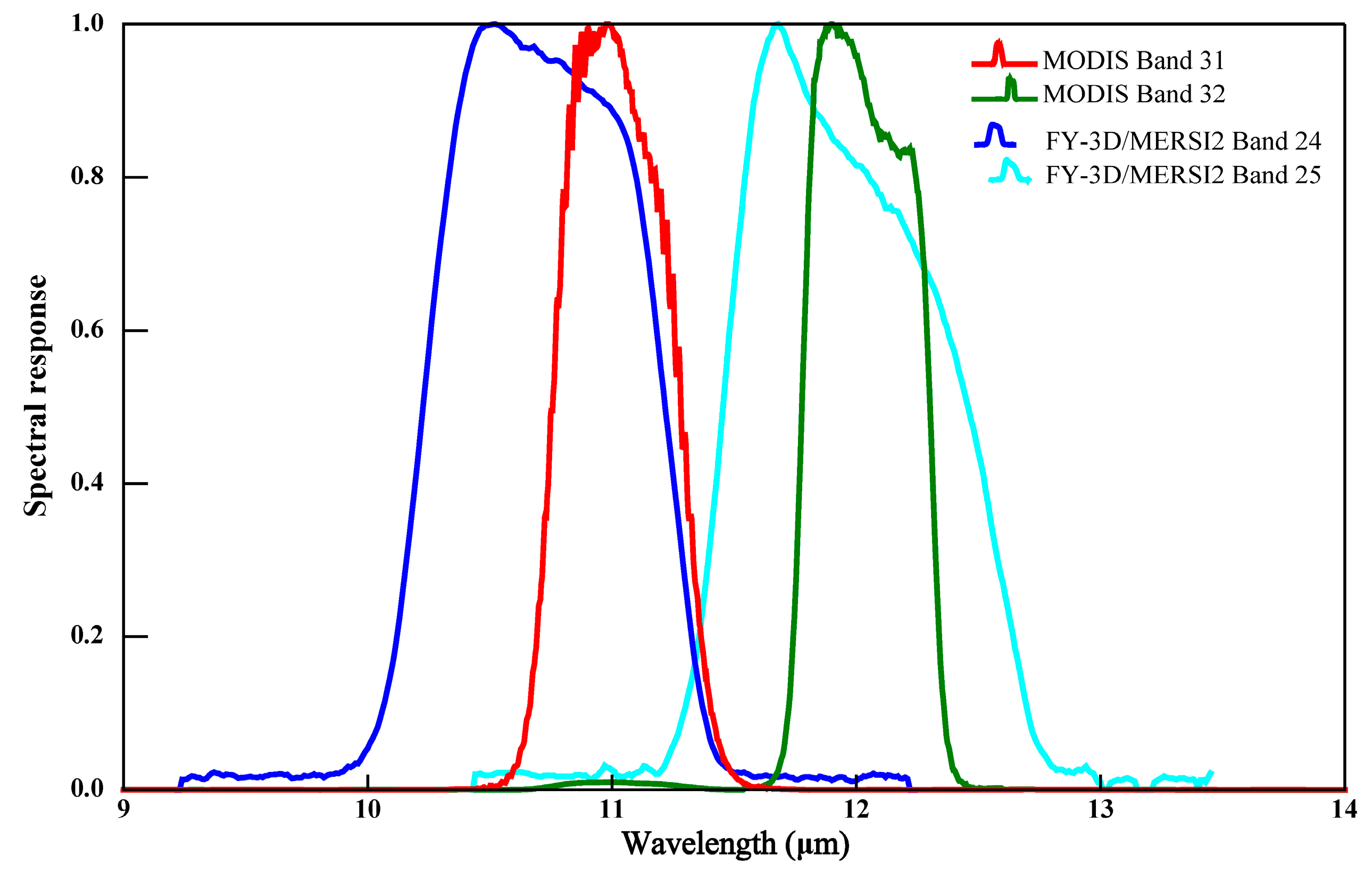
Figure 1 shows the spectral response functions of the MERSI-2 TIR bands (Bands 24/25) and the MODIS TIR bands 31 (10.78–11.28 μm) and 32 (11.77–12.27 μm). As seen in
Table 2 and
Figure 1, TIR band ranges of MERSI-2 and MODIS are similar, and the center wavelengths are close, which indicates the rationality of using MODIS data as one of the cross-calibration and validation references.
2.2. The Research Approach
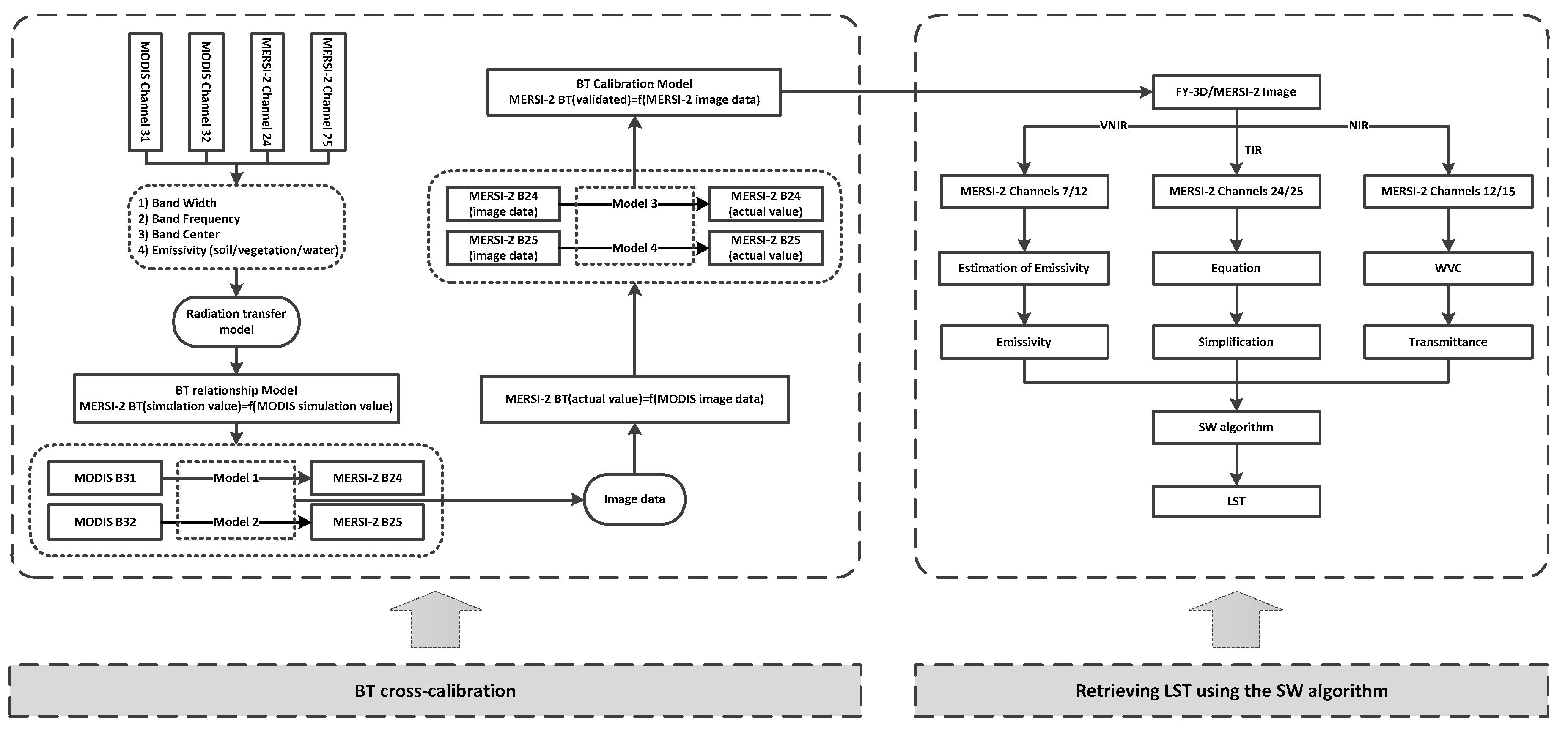
The framework and technical methods of this research are described in
Figure 2. To further explore the possibility of retrieving LST from MERSI-2 data and provide support for the development of an LST product algorithm, the main approach of this study is as follows: first, we propose a method for retrieving LST using the SW algorithm after cross-calibration of the BT and conduct an example application analysis. Second, in the cross-calibration stage, as MERSI-2 and MODIS data have similar imaging times and TIR band range settings (MERSI-2 Bands 24/25 and MODIS Bands 31/32), the MERSI-2 and MODIS simulation data are obtained by using the MODTRAN program to simulate the radiation transfer process, and the BT relationship model (BT Rel-Model) is established to convert the MODIS BT (simulated value) to MERSI-2. Next, according to the BT Rel-Model, the BT calibration model (BT Cal-Model) is established to correct the BT of the MERSI-2 image to the actual value and then calculate the cross-calibrated BT from MERSI-2. Third, in the LST retrieval stage, according to the characteristics of NIR bands, we can retrieve the water vapor content (WVC) and then calculate the atmospheric transmittance from the WVC in the image. The land surface emissivity is estimated by the NDVI-based threshold method so that the main parameters for retrieving the LST from the same image are determined. Finally, we perform a sensitivity analysis for the main parameters (WVC, atmospheric transmittance, and emissivity) in the SW algorithm to evaluate the applicability and promote the application of the algorithm.
3. The Principle of LST Retrieval and SW Algorithm Derivation
3.1. The Principle of LST Retrieval
During transmission through the atmosphere to the satellite sensor, land surface radiation is subject to many disturbances, such as those from the land surface type, soil moisture, near-surface air temperature, and WVC. Therefore, it is a prerequisite to obtain the LST to accurately quantify the mode of interaction between the LST and main interference factors. The derivation of the LST retrieval algorithm is based on the process of land surface heat radiation transfer, which can be quantified as shown in Equation (1) [
27]:
where
denotes the radiance at wavelength
received by the sensors at the top of the atmosphere;
denotes the radiation emitted by the ground objects and is often quantified using the Planck function (Equation (2));
is the land surface emissivity at wavelength
, and
is the reflectance. In addition,
is the atmospheric transmittance at wavelength
from the ground to the remote sensor; and
denotes the upwelling path radiances, while
denotes the downwelling path radiances.
where
indicates the intensity of black radiation (W/m
2µm);
indicates the Planck constant (6.6256 × 10
−34 J·S);
represents the Boltzmann constant (1.38 × 10
−23 J/K);
indicates the speed of light (3 × 10
8 m/s); and
represents the absolute temperature (K).
Based on the lack of influence on the accuracy of the algorithm, an approximate solution can be obtained by Equation (3) (Qin et al. 2001; Mao et al. 2005):
where
represents the average temperature of upward radiance of atmosphere, and
represents the average temperature of the downward radiance of atmosphere. Qin et al. (2001) [
18,
22] concluded that replacing
with has no substantial effect on the calculation of the equation according to the results of an analysis and comparison. Thus, the land surface heat radiation transfer equation can usually be simplified to Equation (4):
The parameters in Equation (4) can be further clarified from left to right: is a known number, and the remaining parameters are unknowns; that is, the equation contains four unknowns.
3.2. The SW Algorithm Derivation
Many scholars have proven the feasibility of using the SW algorithm to retrieve LSTs [
28,
29]. In addition, according to different sensors and research areas, different methods are chosen to simplify and solve the parameters of the thermal radiation transfer equation, to propose different SW algorithms, and implement constant improvements. The general expression of the SW algorithm is as follows:
where is a parameter; and represent the BT of channels
and
, respectively; and the units for
,
, and
are absolute temperatures (K).
Referring to Equation (5) and continuing to solve Equation (4), further simplification is needed. The traditional algorithm involves performing the Taylor expansion on the Planck function and taking one item for simplification. Many studies have proven that linear simplification of the Planck equation is also applicable [
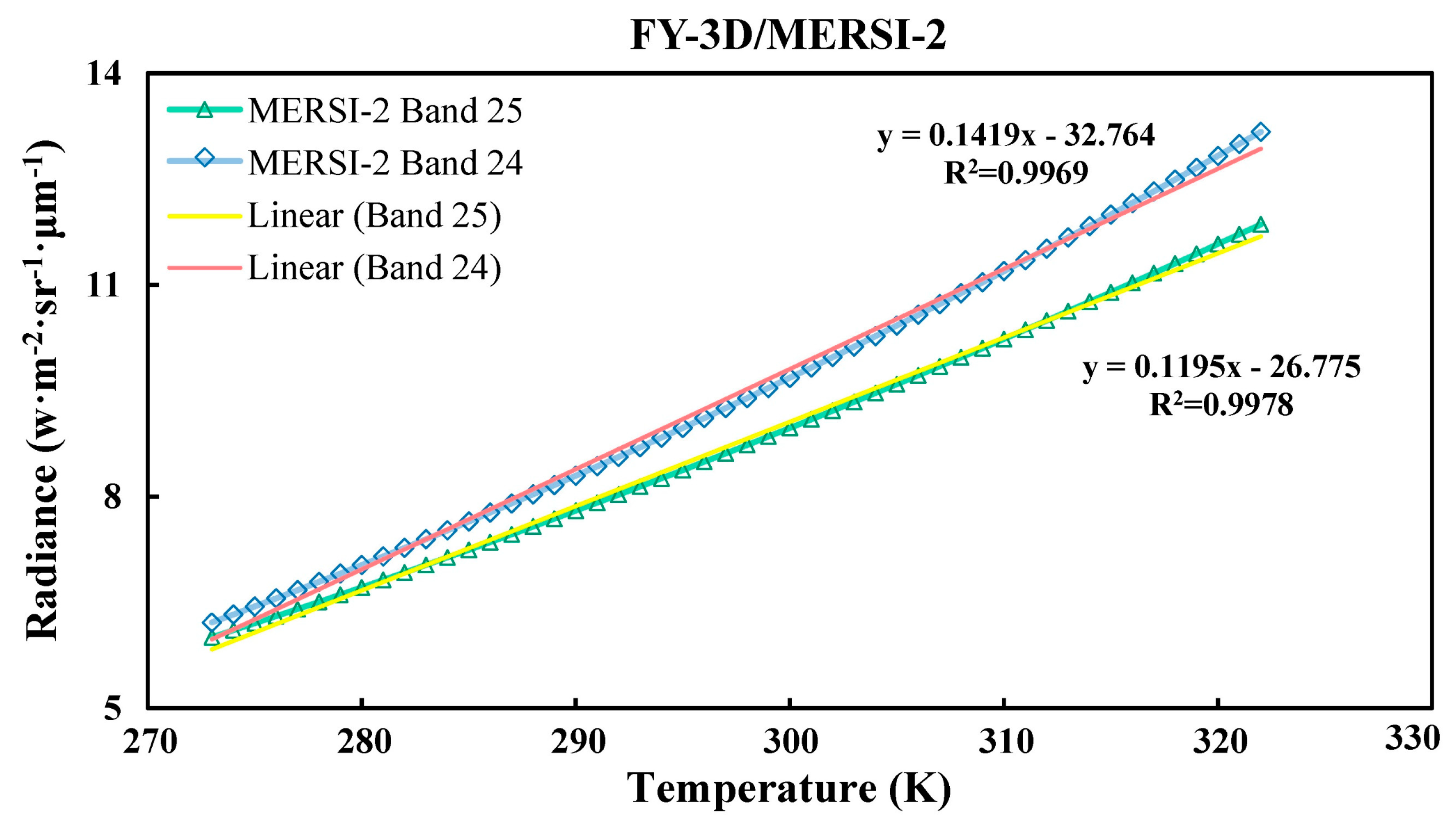
22]. Thus, the correlation analysis between the radiation intensity and temperature for MERSI-2 Bands 24 and 25 is carried out, and the results show that there is an approximate linear relationship between the radiation intensity and the temperature, as indicated by a scatter-plot analysis of the two channels between 273 and 322 K (0–49 °C) (see
Figure 3).
Therefore, the linear regression equation can be substituted for the Planck function for further simplification. The Planck function for MERSI-2 Bands 24 and 25 is reduced as follows:
The results (Equation (6)) of simplifying the Planck function are substituted into the thermal radiation transfer equation (Equation (4)), and we can obtain Equation (7) to calculate LST by the final simplification.
where
To obtain LST, it is necessary to obtain only two parameters: land surface emissivity and atmospheric transmittance . By simplifying the Planck function with the SW algorithm, we can reduce the initial need to obtain three complex unknown parameters to two unknown parameters, which are easier to obtain and greatly simplify the LST retrieval workload while ensuring high accuracy.
4. Practical Example Analysis
To perform an application analysis, we selected a MERSI-2 image from August 3, 2018 (UTC 4: 40) and a MODIS image from August 3, 2018 (UTC 4: 20). During the hot summer, the vegetation in the Bohai Sea area of China is prosperous and the ground recognition conditions are sufficient. The MERSI-2 image was radiometrically scaled, reflectivity calibrated, geometrically corrected, and cross-calibrated to obtain the effective BT, reflectivity, and other information. Finally, the SW algorithm was used to analyze the spatial differences in LST and heat in this area.
4.1. BT Cross-Calibration
Through our analysis, we found that the BT detected by the MERSI-2 instrument deviated greatly from the actual value. To determine the reasons, we can think from the following two aspects: on one hand, the MERSI-2 sensor may be offset; on the other hand, the TIR data from MERSI-2 need to be further improved via laboratory calibration and field calibrations, which also hinders the development of MERSI-2 TIR data into allow for use in more applications. If no cross-validation is conducted, it is nearly impossible to retrieve LSTs. Furthermore, MODIS LST products are widely used and have been calibrated by NASA for many years, providing an accurate reference object for LST retrieval. To further improve the LST retrieval accuracy, we propose a method using the SW algorithm after cross-calibration of the BT of MERSI-2 TIR bands (Bands 24/25). Accordingly, in the BT cross-calibration stage, two important models are established in this study: the BT relationship model (BT Rel-Model) and the BT calibration model (BT Cal-Model).
4.1.1. BT Relationship Model Establishment
MERSI-2 has imaging times that are similar to those of the MODIS data as well as similar TIR range settings (MERSI-2 Band 24 and MODIS Band 31, MERSI-2 Band 25 and MODIS Band 32). To improve the accuracy of radiation correction, we used the MODTRAN program to simulate the radiation transfer process to obtain MERSI-2 and MODIS simulation data in the mid-latitude region, and the BT Rel-Model was established between the BTs of MODIS and MERSI-2. As one of the key parameters of LST, land surface emissivity is mainly determined by the land surface type and the band intervals of the remote sensor. Thus, at a spatial resolution of 1 km, the pixels in the Bohai Sea area can be divided into soil, vegetation, and water.
More concretely, the first step is to obtain the BTs of the MERSI-2 and MODIS data in TIR bands. We used the MODTRAN to simulate the radiation transfer process and set the temperature (290–320 K, step length is 1 K), WVC (0.4–3.5 g/cm2, step length is 1 g/cm2), and land surface emissivity (vegetation, water, and soil) values, for a total of 2976 groups of data. Furthermore, we used the PHP program to use MODTRAN to calculate the BTs of MERSI-2 and MODIS.
The land surface emissivities
,
, and
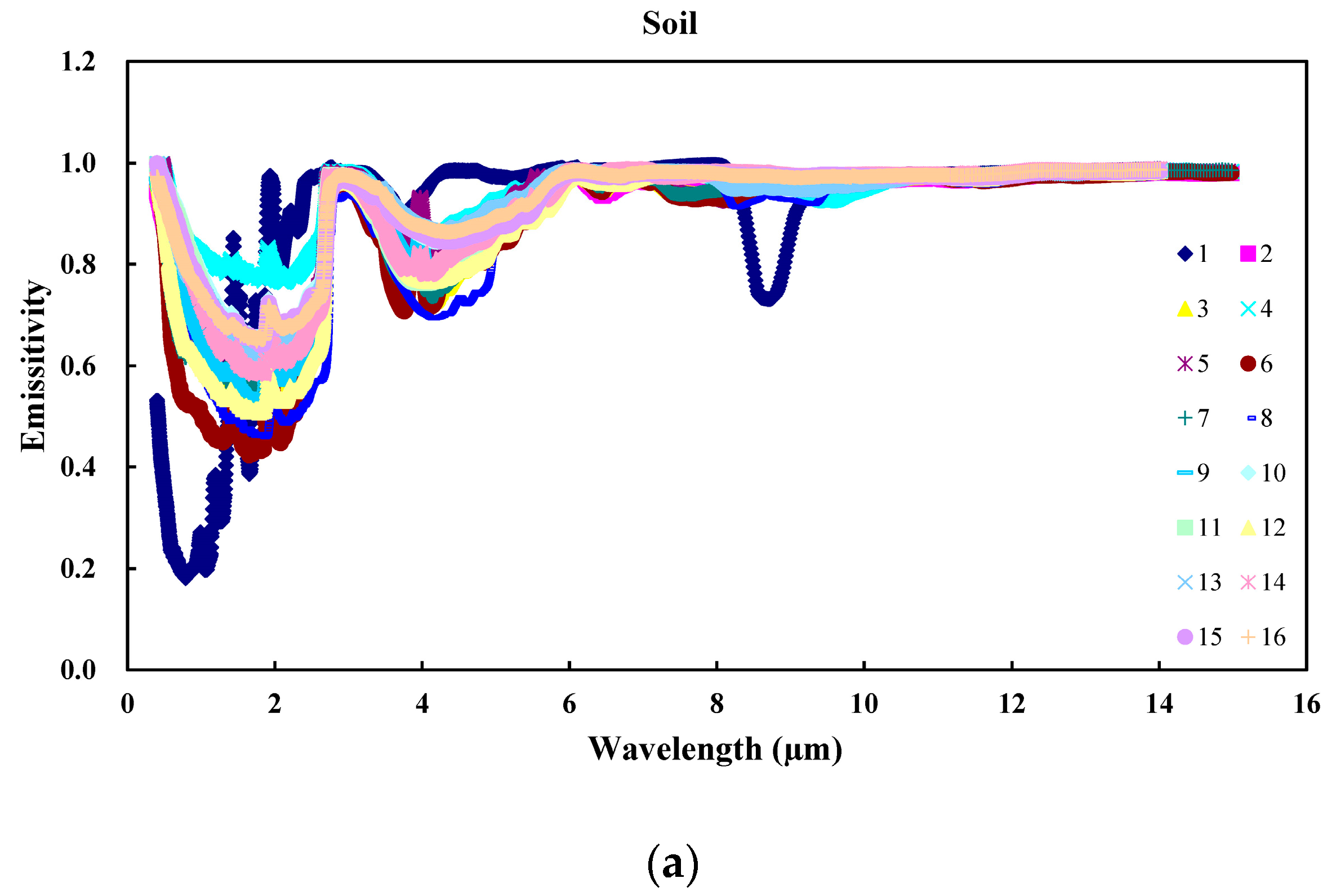
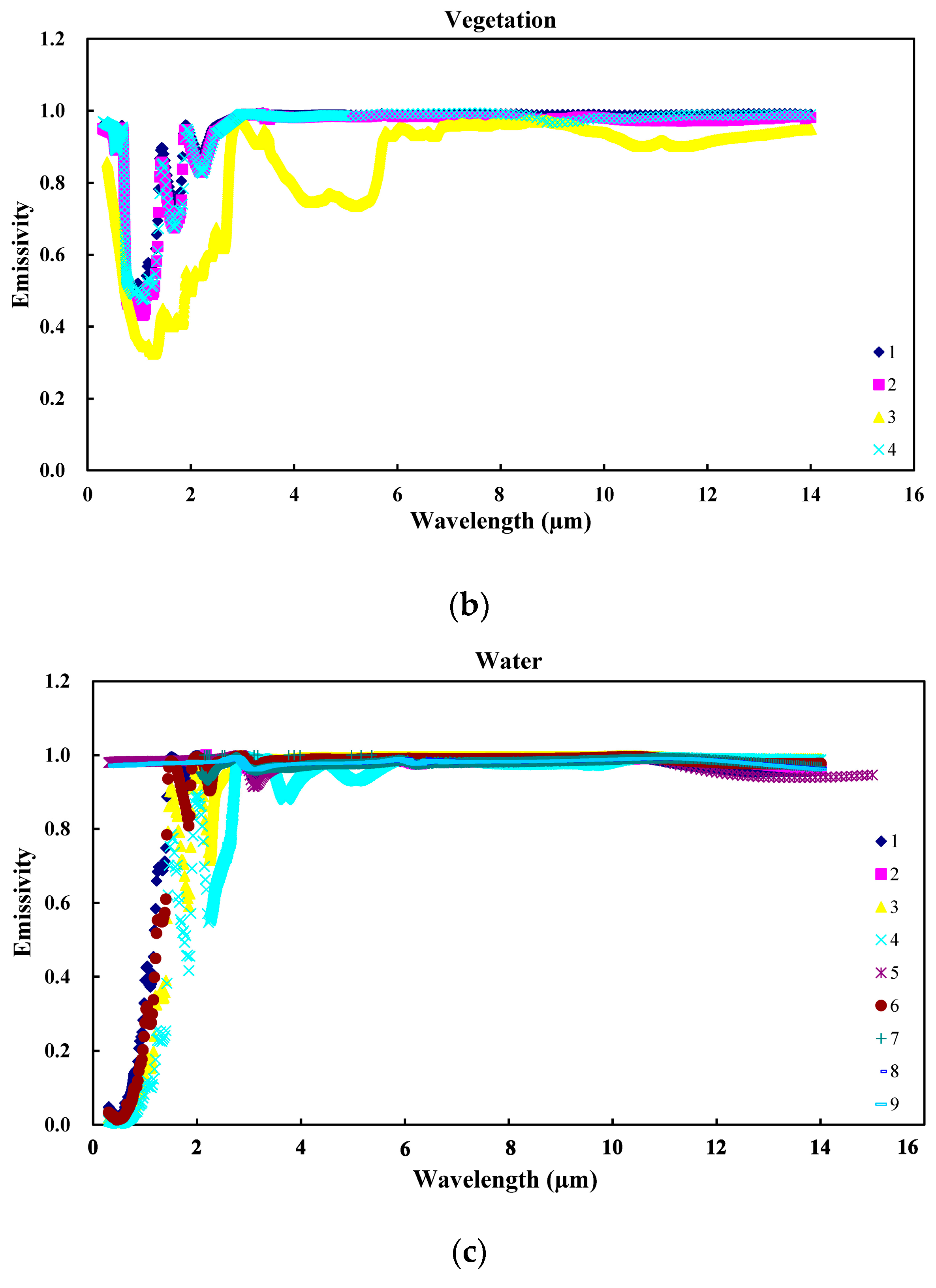
for water, vegetation, and soil, respectively, are usually based on the spectral reflectivity of the ground object, such as the reflectivity spectrum library of ground objects. Therefore, according to the experimental statistics of a variety of soil, vegetation, and water measured reflectivities (as shown in
Figure 4) provided by the Jet Propulsion Laboratory (JPL: URL
http://speclib.jpl.nasa.gov), we selected their average value to represent the land surface emissivities of various objects, where the input of the relevant parameters can be referred to as the technical roadmap (
Figure 2) and
Table 3.
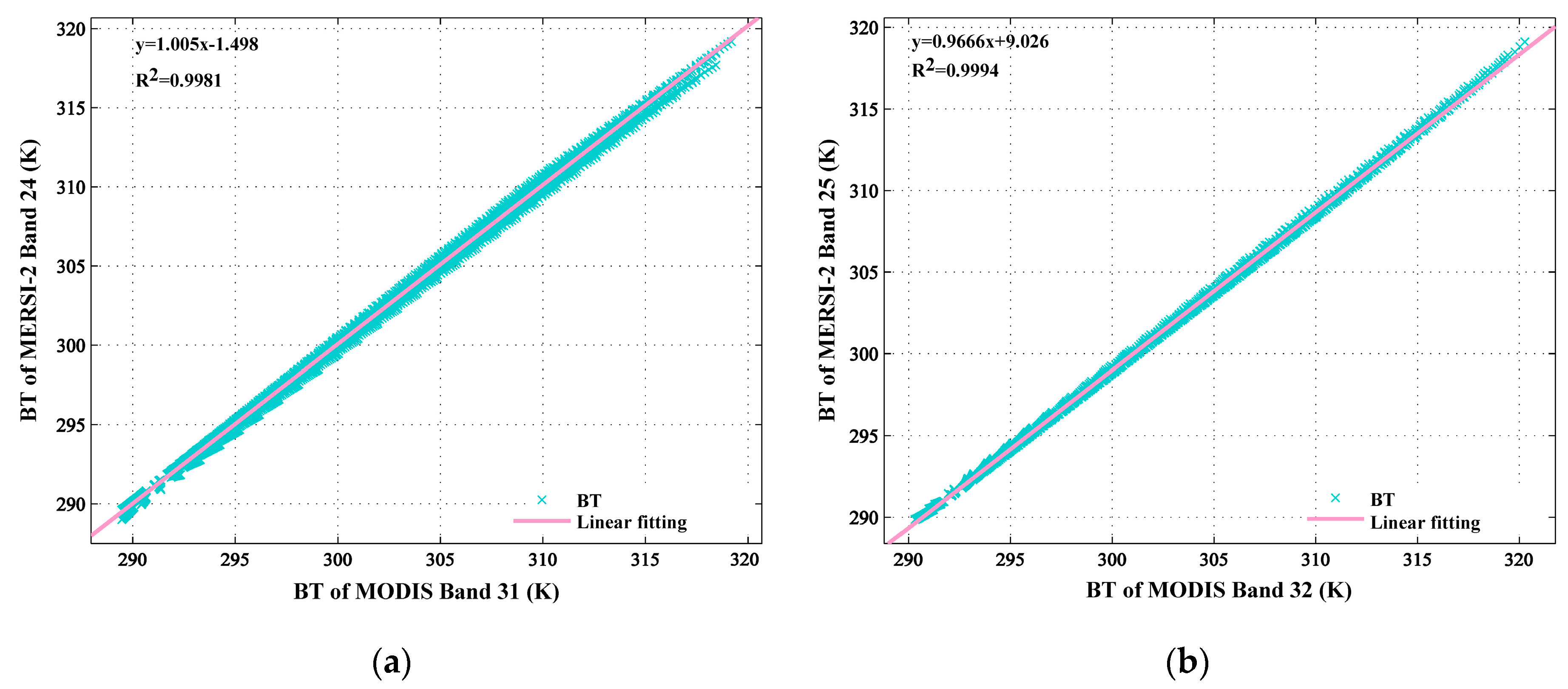
Sampling statistics and regression analysis of the MERSI-2 and MODIS BT simulation results (as shown in
Figure 5) and the correlation coefficients are very high (both over 0.998).
The second step is to build the BT Rel-Model using the simulation data, MERSI-2 BT =f (MODIS), and the MERSI-2 BT can be obtained from the MODIS BT. Additionally, we further subdivided the model into Model 1 and Model 2, as shown in Equation (9):
The simulation results show that with Model 1, we can approximately convert the BT of MODIS Band 31 to the BT of MERSI-2 Band 24; with Model 2, we can approximately convert the BT of MODIS Band 32 to the BT of MERSI-2 Band 24. In the same way, this law can also be applied to images. For example, with Model 1, we can convert the BT of the MODIS Band 31 image to the BT of the MERSI-2 Band 24 image.
4.1.2. BT Calibration Model Establishment
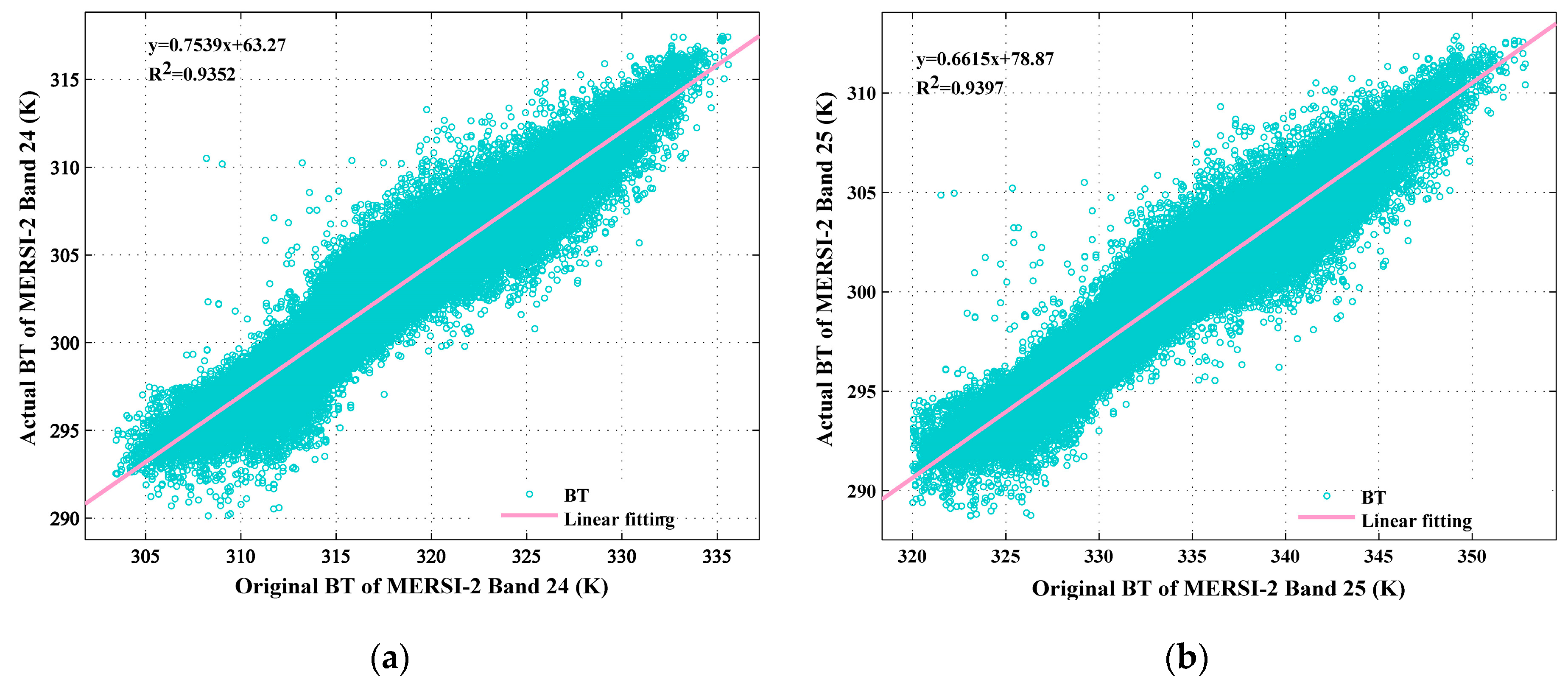
During the establishment of the BT Cal-Model, we convert the BT of the MODIS image to the actual BT of MERSI-2 according to the BT Cal-Model. Next, the statistical analysis of the BT of the MERSI-2 image and the BT converted from MODIS (
Figure 6) indicated that the BT of the MERSI-2 image is much higher than the real situation, and the correlations are very high (all greater than 0.93).
Therefore, we established a validation model that converted the BT of the MERSI-2 image to the actual value, MERSI-2 BT (actual value) = f (MERSI-2 image data), which could be subdivided into Model 3 and Model 4, as shown in Equation (10):
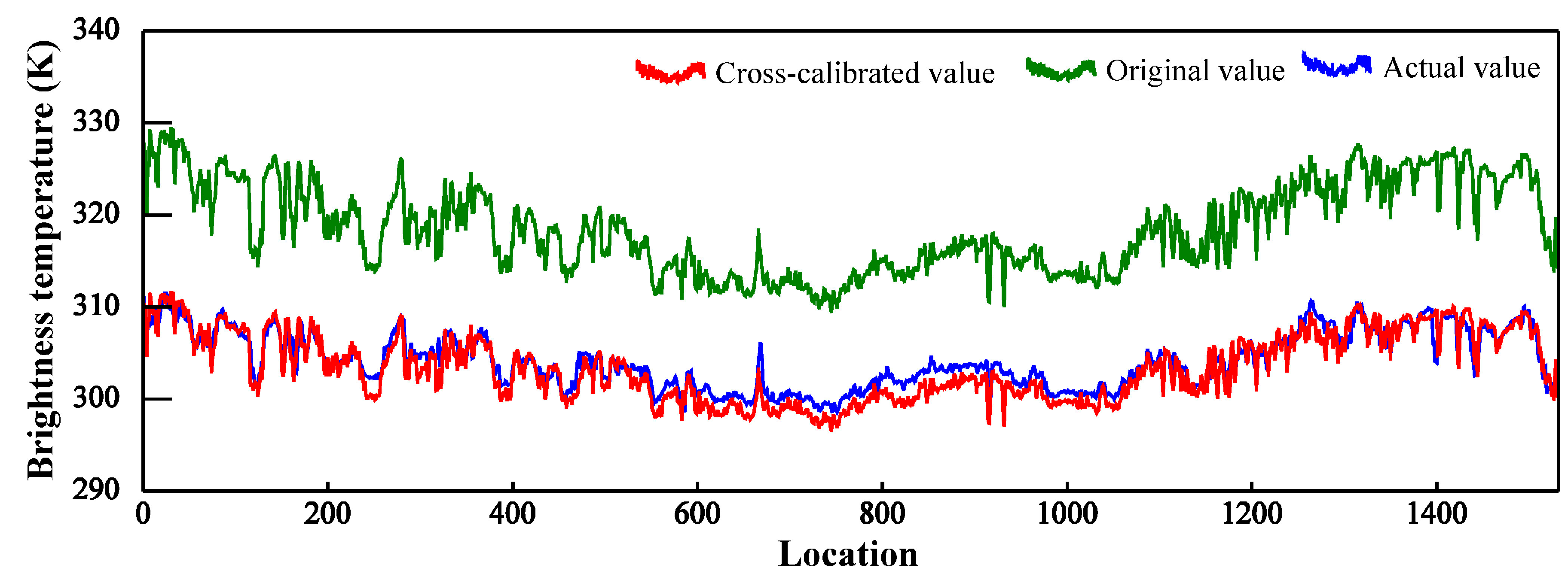
Currently, we can use Model 3 to correct the BT of a MERSI-2 Band 24 image to the cross-calibrated value based on its actual value. Similarly, we can use Model 4 to modify the BT of the MERSI-2 Band 25 image to the cross-calibrated value. As shown in
Figure 7 and
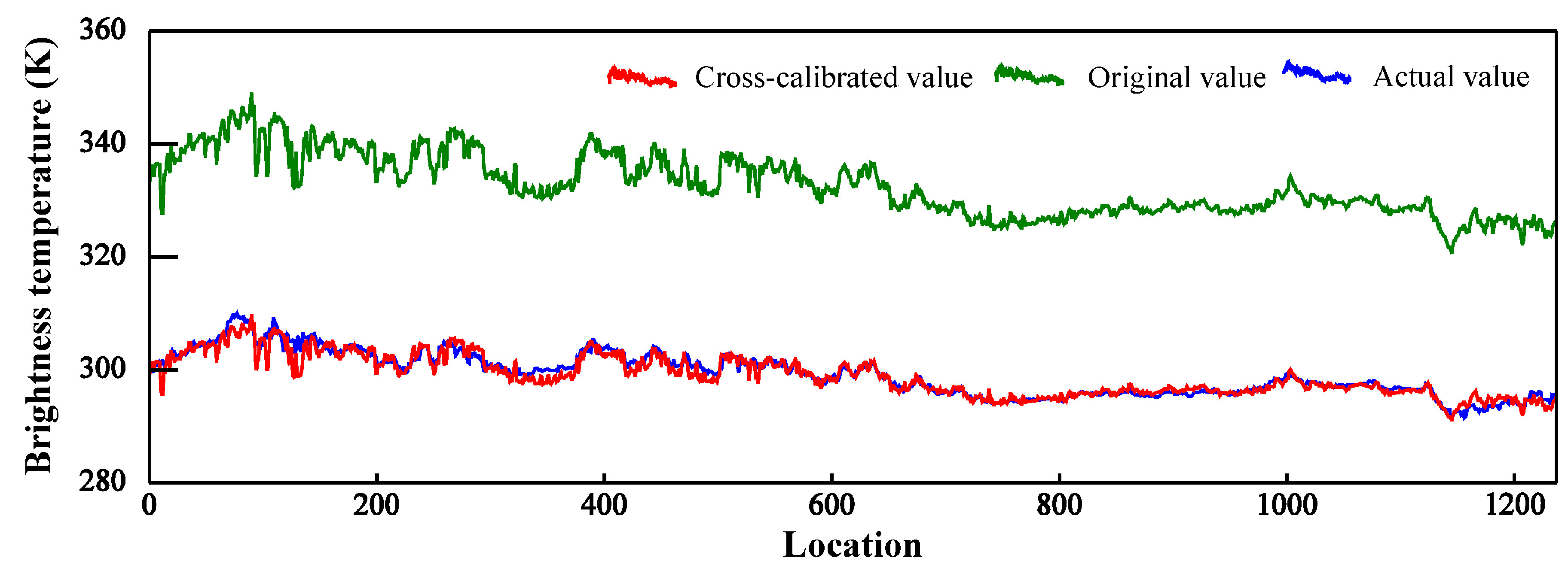
Figure 8, by sampling the statistics, the relationships between the original, actual, and cross-calibrated values of the BT of the MERSI-2 image can be compared to obtain the following conclusion: the original value is higher than the actual value, but after correction by the cross-calibration method, the cross-calibrated value is basically consistent with the actual value.
4.2. Estimation of WVC and Atmospheric Transmittance
Atmospheric transmittance is an important factor in the radiation transfer process, and it is also one of the input parameters in the SW algorithm. For technical reasons, atmospheric transmittance is difficult to obtain in real time, so how to accurately and efficiently estimate atmospheric transmittance has become the focus of many scholars. However, since the WVC is the main factor affecting atmospheric transmittance, the atmospheric transmittance can be obtained by establishing the relationship between the WVC and atmospheric transmittance. As a general rule, two main methods are used to establish this relationship. The first method is to estimate the WVC by using the measured data from a ground meteorological detection site to estimate the atmospheric transmittance. However, the land surface meteorological stations are unevenly distributed and affected by the topography, so the point-like water vapor data cannot accurately reflect the regional conditions. The second method is to use real-time atmospheric data to obtain the WVC and calculate atmospheric transmittance through radiation transfer process software such as MODTRAN, 6S, or LOWTRAN. With this method, it is also difficult to obtain the atmospheric profile data synchronized with the image to ensure the accuracy of the simulation results. Therefore, it is better to obtain WVC and atmospheric transmittance from the same remote sensing image.
4.2.1. Estimating WVC from NIR Bands
Among the 25 bands of MERSI-2, six NIR bands are provided, and the atmospheric windows include Band 11 (0.855–0.875 μm), Band 12 (0.84–0.89 μm), and Band 16 (1.23/1.02–1.25 μm). The water vapor absorption bands include Band 13 (0.895–0.915 μm), Band 14 (0.926–0.946 μm), and Band 15 (0.915–0.965 μm). Therefore, we can estimate the WVC directly from the same remote sensing image through NIR bands and then estimate the atmospheric transmittance to meet the accuracy and real-time requirements of parameter estimation.
After performing experiments, Kaufman et al. (1992) [
30] found that it is feasible to use the ratio method to estimate the WVC, and many studies have proven the feasibility of this method [
22,
31]. The two ratio methods are calculated as follows:
where
= 0.8,
= 0.2, and the weight assignment can be adjusted according to the situation;
is the water vapor absorption band;
and
are the atmospheric windows; and
is the reflectance of the band. The principle for the above two ratio methods is the same: in NIR bands, the ratio of the water vapor absorption band reflectance to the atmospheric window reflectance is approximated as the atmospheric transmittance. For the relationship between the atmospheric transmittance and the WVC, we can simulate and establish their relational expressions (Equations (13) and (14)) by using the MODTRAN program.
In Equations (13) and (14), for complex surfaces,
,
, and the other land surface conditions are shown in the study of Kaufman et al. [
30]. Thus far, we have estimated the WVC from NIR bands.
4.2.2. Estimating Atmospheric Transmittance from WVC
In the previous section, we calculated the WVC in NIR bands. From this information, we can simulate the atmospheric transmittance of TIR bands with the change in WVC through the MODTRAN program and then establish a model to estimate the atmospheric transmittance from the WVC. Therefore, the changes in the atmospheric transmittance of MERSI-2 Bands 24 and 25 with WVC in the summer midlatitude atmosphere are shown in
Figure 9 below.
Figure 9 indicates that with the increase in WVC, the atmospheric transmittance shows a decreasing trend. After linear fitting and polynomial fitting, we selected the results of the cubic polynomial fitting (as shown in Equation (15), which had the highest correlation, to approximate the relationship between the atmospheric transmittance and the WVC in TIR bands:
Thus far, it is possible to synchronously retrieve the WVC and the atmospheric transmittance in the same image, thereby greatly improving the accuracy and real-time performance of LST retrieval.
4.3. Estimating Land Surface Emissivity by Using the NDVI-Based Threshold Method
As one of the key parameters of LST, land surface emissivity is mainly determined by the land surface type and the band intervals of the remote sensor. The calculation of land surface emissivity based on NDVI values is a simple and effective method that has been applied and validated in many studies [
31,
32,
33,
34]. According to Mao’s (2005) [
22] idea for estimating the land surface emissivity from MODIS images with 1 km spatial resolution, the MERSI-2 image pixels in the Bohai Sea area can also be divided into soil, vegetation, and water. Therefore, Equation (16) is often used to roughly estimate the land surface emissivity of the MERSI-2 mixed pixels:
where
represents the land surface emissivity of the mixed pixels,
,
and
are the land surface emissions of water, vegetation, and soil, respectively;
,
, and
are the proportions of water, vegetation, and soil in the mixed pixels, respectively; and
,
, and
are temperature ratios, and their calculation formula is
. In addition, Qin (2004) [
35] estimated the typical ground temperature ratio to be within the range of 5–45 °C. Therefore, we estimate the average temperature ratios of the three types of land surfaces as
,
and
.
There have been many studies on the NDVI-based threshold method, and the threshold values set for vegetation, water, and soil differ among studies, but the research principles are consistent. If there are obvious vegetation, water, and soil areas in the image (approximated as pure pixels), we can take the average value of NDVI in this area as the threshold, namely,
,
and
. Therefore, when the NDVI of a mixed pixel is greater than the threshold, we take
; otherwise, we calculate the ratio of the three features (vegetation, water, and soil) in the mixed pixel. In most studies [
22,
34,
35], the NDVI value of dense and healthy vegetation is greater than 0.5, the NDVI of water is less than 0, and the NDVI value of bare soil is usually in the range of 0.03–0.2. In this study, the NDVI values of obvious water, vegetation, and bare soil areas are statistically analyzed; finally, we obtained
,
and
.
In the mixed pixels, the ratio of water in the near-coast pixels can be estimated by
, where QDN is the DN of the pixels, and DN1 is the smallest DN of the land pixels. For land pixels, we can determine the vegetation coverage based on the NDVI value, as shown in Equations (17) and (18) [
22]:
Regarding the land surface emissivity values of water, vegetation, and soil (
), according to the experimental statistics of the variety of soil, vegetation, and water measured reflectivity values (as shown in
Figure 4), we select their average values as the land surface emissivity; that is, for MERSI-2 Band 24, we take
,
, and
, and for MERSI-2 Band 25, we take
,
, and
.
4.4. Retrieval Results and Analysis
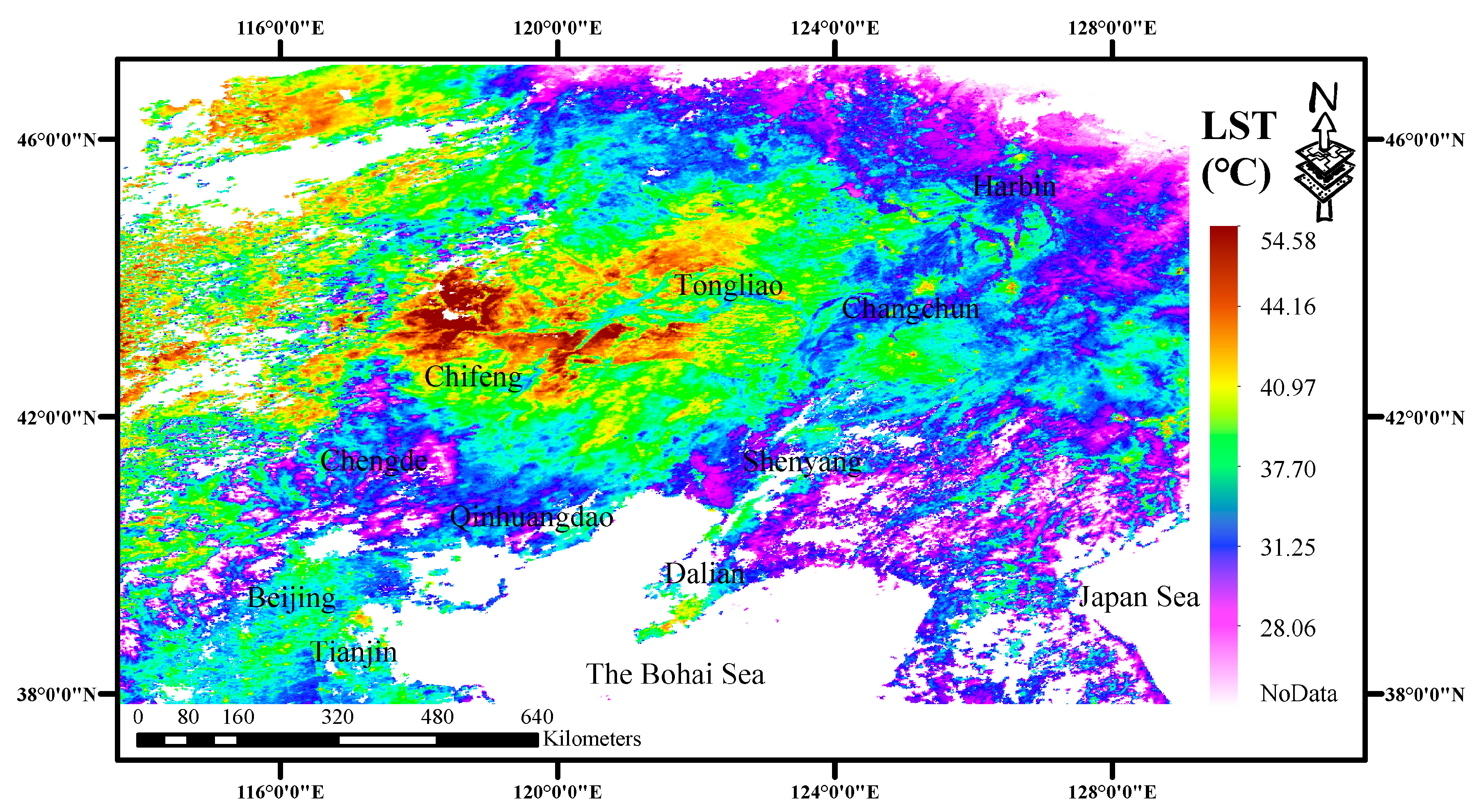
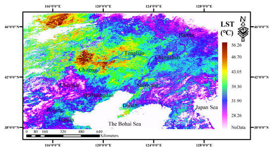
To date, we have determined three unknown parameters involved in the SW algorithm solution: atmospheric transmittance, land surface emissivity, and BT (cross-calibrated). We substitute these equations into the SW algorithm (Equation (7)) to obtain the LST retrieval results in the Bohai Sea area, as shown in
Figure 10.
According to the LST retrieval results (
Figure 10), we can obtain the following information: (1) The LST ranges from 18.98–56.26°C and the geometric information and temperature values are within the reasonable range for summer LST. (2) The urban heat island effect is prominent, and from north to south, we can clearly identify central cities such as Harbin, Changchun, Shenyang, Dalian, Beijing, and Tianjin. The temperatures of these urban centers are generally higher than those of the surrounding areas, showing the phenomenon of a temperature decrease from the center to the surrounding areas. (3) We can also identify the northwestern region of Qinhuangdao (such as Chengde) and the dense vegetation area adjacent to the Japanese sea area because the temperatures in these areas are slightly lower than those in the surrounding areas, while the Tongliao and Chifeng areas are sparsely populated, and their temperatures are also the highest.
4.5. Validation
Validation of the algorithm is indispensable before the algorithm is promoted and applied. On the whole, there are three main methods for the validation of the algorithm for LST retrieval. The first method is to simulate the atmospheric radiation transfer process through atmospheric modeling software such as LOWTRAN or MODTRAN and evaluate the accuracy of the algorithm based on the obtained data. The second method is to compare the LST retrieval results with mature LST products and then evaluate the relative error. The third method is to use data measured from ground monitoring sites to evaluate the accuracy of the LST retrieval. However, these three evaluation methods have their own limitations: (1) The first method evaluates only the average accuracy and does not fully reflect the real ground thermal radiation transfer process during satellite transit. (2) The second method is very strict in terms of the imaging time of the sensors for comparison and is more suitable for comparison between data with similar imaging times. (3) For the third method, it is difficult to provide observation data synchronized with the satellite, and the point data do not easily reflect the spatial differentiation of the regional temperature. Therefore, to comprehensively evaluate the algorithm and retrieval results proposed in this study, the above three evaluation methods will be used to evaluate the accuracy.
4.5.1. Validation through a Standard Atmosphere Simulation
In this study, the principle of using the MODTRAN program to simulate the radiation transfer process is to input parameters such as spectral bandwidth, frequency, and center wavelength of MERSI-2 Bands 24/25 and set the LST, WVC, land surface type, and land surface emissivity values. According to this method, the process of thermal radiation conduction at the land surface for the atmospheric conditions in the midlatitude region can be simulated; finally, we can obtain the following six types of output parameters: set LST, WVC, atmospheric transmittance, irradiance, surface type (emissivity of vegetation/water/soil), and BT. Further work involves recalculating the atmospheric transmittance and obtaining the actual value of the LST using the transmittance polynomial estimation model and the SW algorithm derived in this study. By comparing the actual value with the set LST, we can obtain the average accuracy of the SW algorithm, as shown in
Figure 11.
In
Figure 11, Tr is the transmittance. Through simulation, we obtained 2976 sets of data, which can reasonably evaluate the precision of the SW algorithm, and some of the process data and results are shown in
Table 4 and
Table 5.
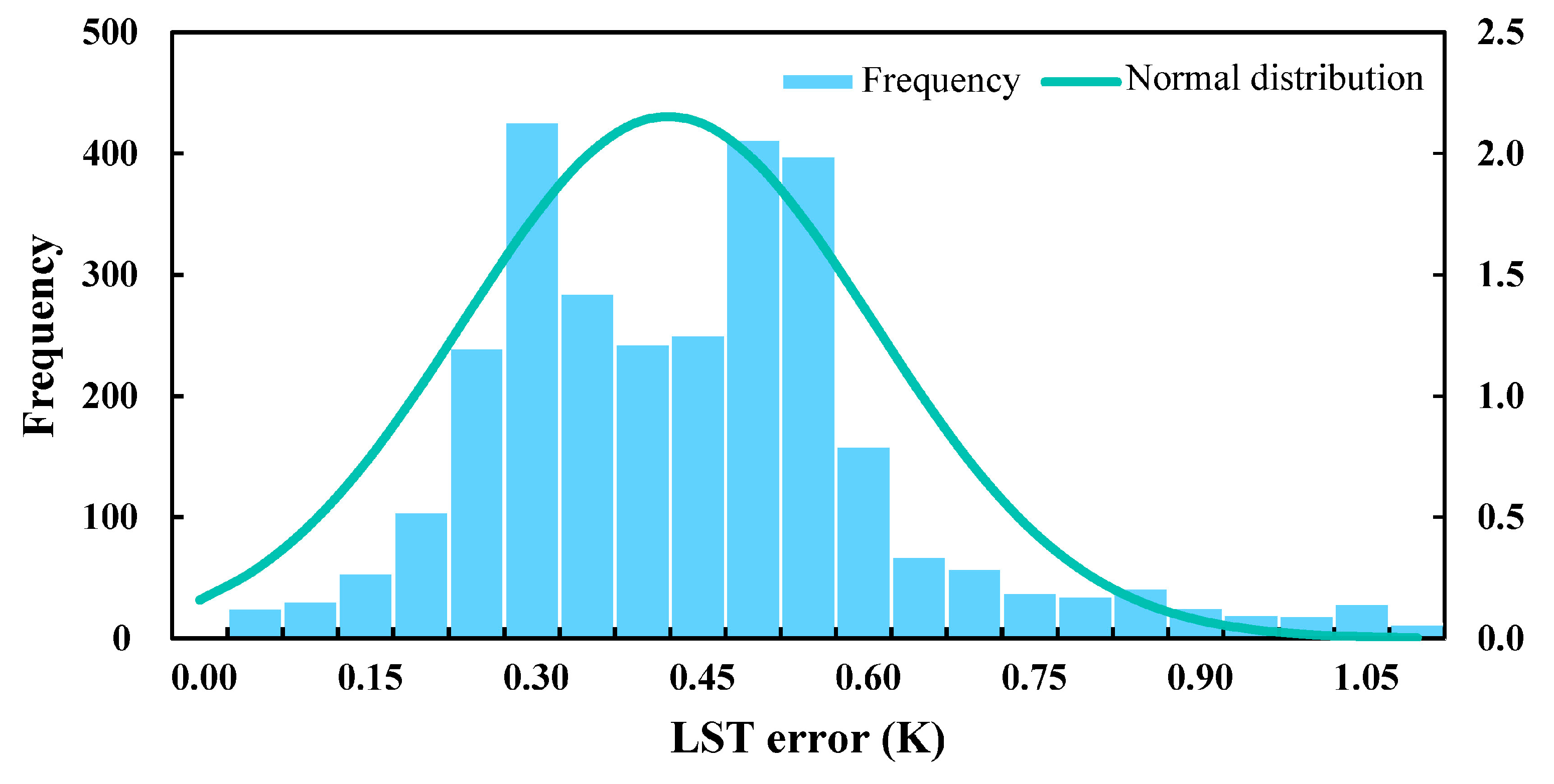
Generally, the average accuracy of our algorithm is 0.42 K when using simulation data, and the RMS is 0.19. In addition, the error distribution frequency and normal distribution curve for the SW algorithm are shown in
Figure 12, which indicates that the SW algorithm proposed in this study has good accuracy and applicability.
4.5.2. Comparison with MODIS LST Products
Although it is difficult to evaluate LST retrieval results based on measured data, Wan et al. (2004) [
36] performed extensive work and verified the MODIS LST products with measured data. The results show that the accuracy of the MODIS LST products in the experimental area is within 1 °C. Therefore, we select the MODIS LST products (MYD11A1, as shown in
Figure 13) provided by NASA and the results of the MERSI-2 retrieval results using the SW algorithm for relative error analysis.
As shown in
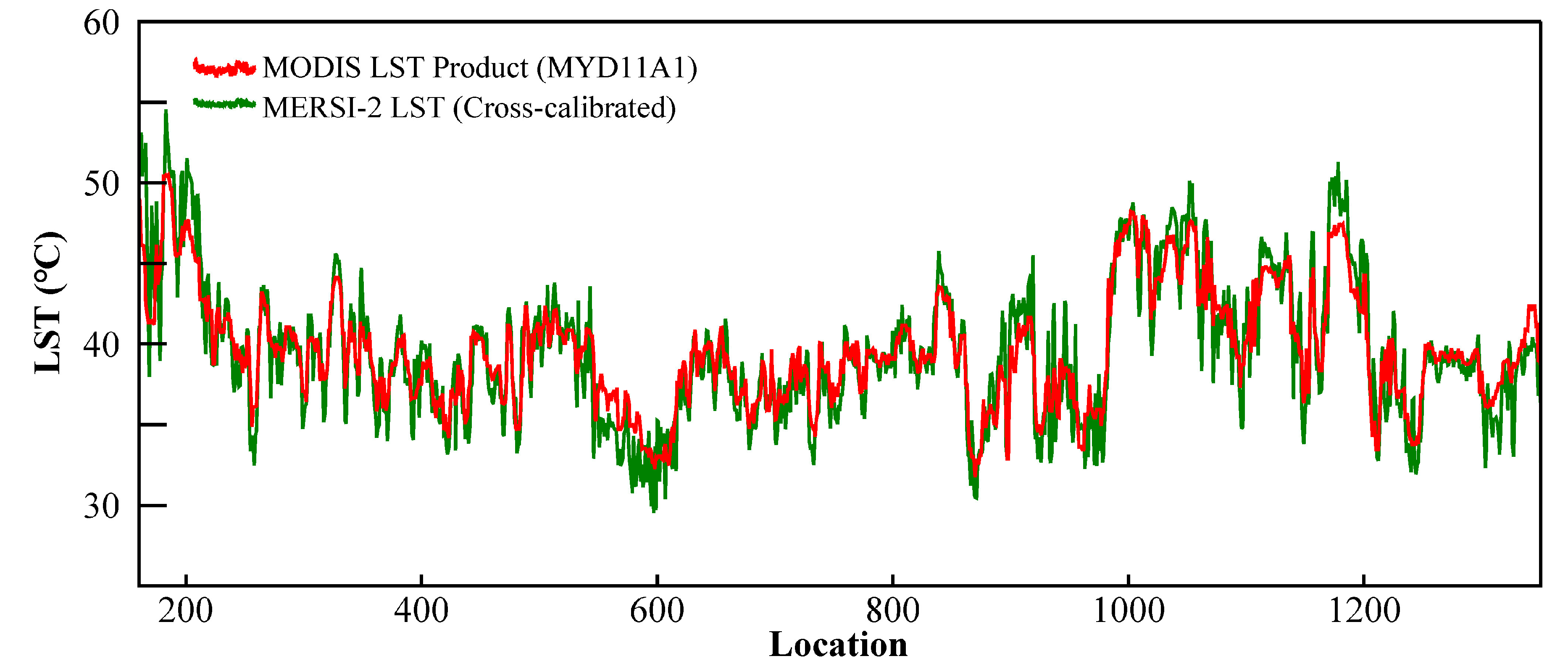
Figure 13, the values from MODIS LST product (MYD11A1) ranges from 13.48–54.58 °C; that is, the retrieval result of MERSI-2 is basically consistent with the spatial heterogeneity of the MODIS LST product at high, medium, and low temperatures. Through our analysis of the LST profile under clear sky conditions in the images (as shown in
Figure 14), the LST trends of MERSI-2 and the MODIS LST product are basically the same, while the average temperature error is 1.37 K, and the RMS is 1.17. The imaging times of MODIS and MERSI-2 are close but not the same, and the MODIS LST products have some errors compared with the real LST. Therefore, when we compare the retrieved LST of MERSI-2 with MODIS LST products, the final results are only the spatial analysis of the LSTs and relative errors and are not absolutely precise.
4.5.3. Comparison with Ground-Measured Data
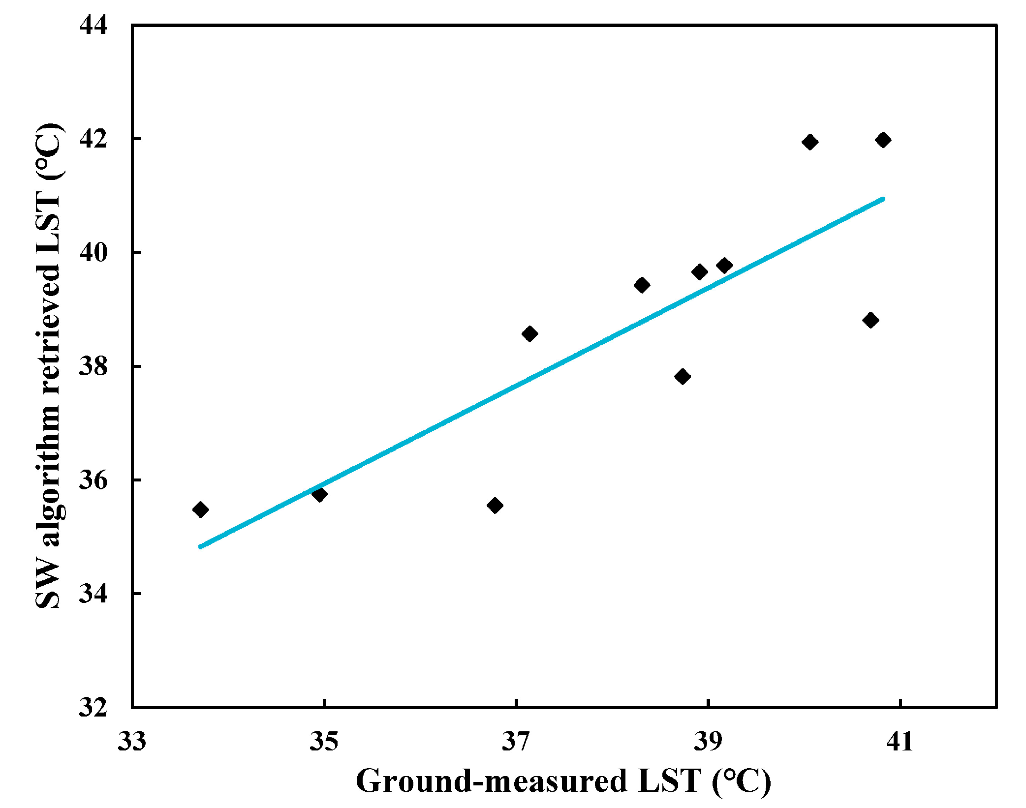
It is not ideal to evaluate the spatial distribution of LST over a large scale by using point-like measured data. On one hand, it is difficult to obtain ground data that is consistent with the resolution of image pixels when satellites are in transit, and on the other hand, it is difficult to obtain parameters such as real-time atmospheric profile data. Therefore, we consider this method only for evaluating the results and algorithm accuracy of LST retrieval. The ground monitoring station data were obtained from the China Meteorological Administration. After quality control, 11 representative stations with single ground land cover types and flat terrain, which had imaging times close to those of the MERSI-2 data, were selected to evaluate the accuracy of the proposed algorithm. As shown in
Figure 15, the evaluation results show that the accuracy of the SW algorithm is 1.23 K, and the RMS is 0.46. In general, the accuracy of the algorithm is relatively high, but the algorithm still requires further improvement in subsequent research.
5. Discussion
Parameter sensitivity analysis is very important in algorithm development and practical applications. In the SW algorithm, emissivity and transmittance are the main influencing factors, and WVC is the factor that influences atmospheric transmittance. Therefore, the sensitivity analysis on the three main influencing parameters, namely, WVC, atmospheric transmittance, and emissivity, was carried out. Equation (19) can approximately evaluate the effect of parameter errors:
5.1. Sensitivity Analysis of WVC
In the SW algorithm, the atmospheric transmittance is estimated from WVC, so the sensitivity of the algorithm to the WVC determines the applicability of the algorithm. In this study, the MODTRAN program is used to simulate the radiation transfer process (see
Figure 11) to obtain standard atmospheric simulation data for analyzing the sensitivity of WVC.
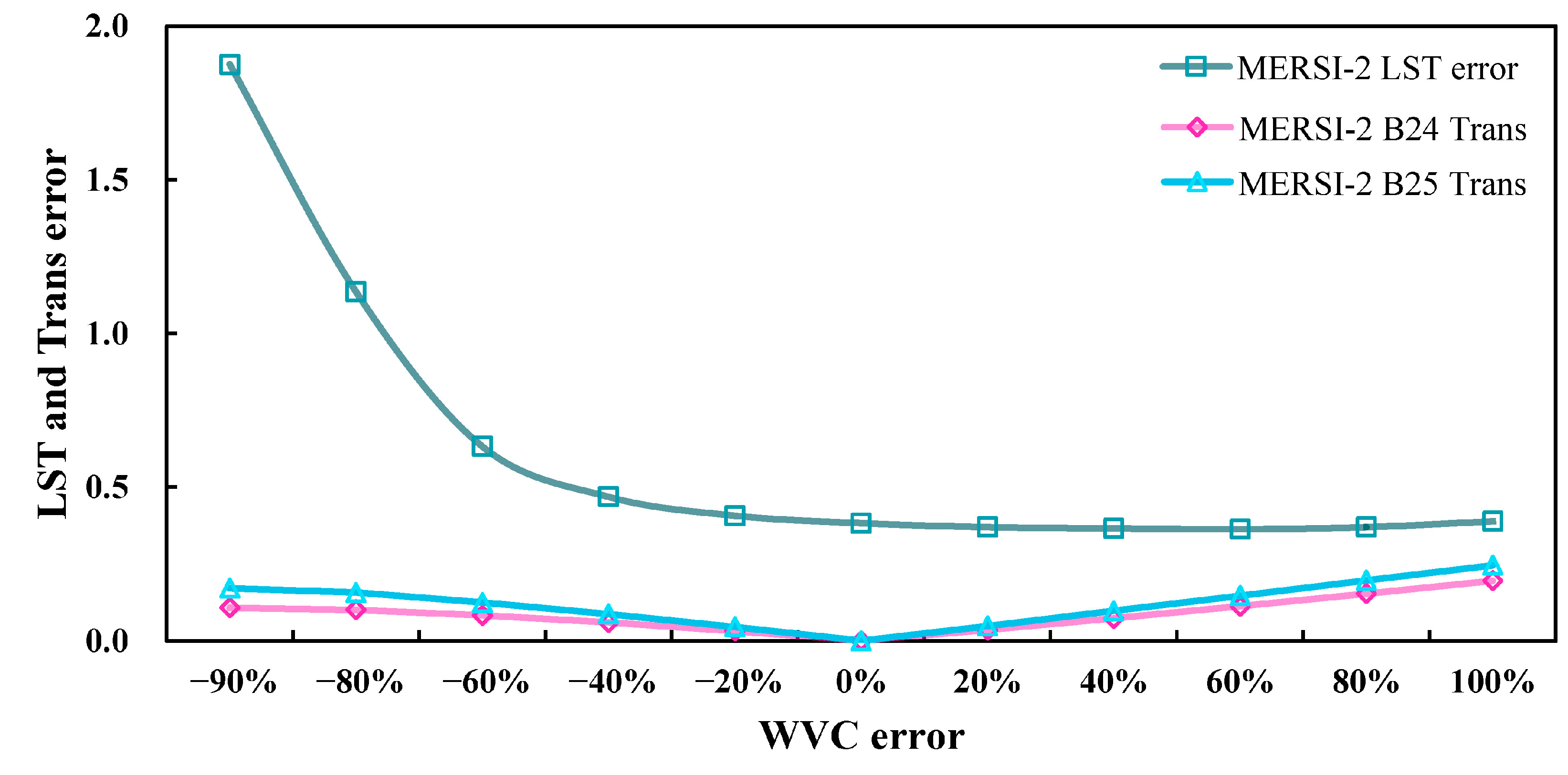
Table 6 shows the partial LST inversion results obtained by changing the WVC error (−90–100%). From
Table 6, we can also obtain the change in transmittance with the variation in WVC errors (−90–100%), where the LST error represents the difference between the retrieved LST before and after the change, and the RMS represents the root mean square.
From
Table 6 and
Figure 16, we can obtain the following information: (1) When there is no change in WVC (0%), the transmittances of MERSI-2 Bands 24 and 25 are 0.85 and 0.77, respectively, while the average LST error is 0.38, and the RMS is 0.13. (2) When the WVC error is 60%, the average transmittance errors of MERSI-2 Bands 24 and 25 are 0.11 and 0.15, respectively, and the accuracy of the LST retrieval is the highest (LST error is 0.36 K, and the RMS is 0.14). (3) When the WVC error is between −20% and 100%, the average transmittance error of MERSI-2 Bands 24 and 25 is between 0 and 0.2, while the mean LST error is very small (all less than 0.5 K) and the trend is stable; that is, the algorithm is not sensitive to the WVC.
Kaufman and Gao (1992) [
30] retrieved the WVC from MODIS under clear weather conditions with a maximum inversion error between −13% and +13%. Considering that MERSI-2 and MODIS have similar TIR band settings, the sensitivity analysis of the WVC for MERSI-2 can be analyzed with reference to the sensitivity analysis of MODIS. Finally, we obtain the following results: the algorithm proposed in this study is not sensitive to WVC, which proves that it is feasible to use this algorithm to estimate the transmittance from WVC, and the practicability of the SW algorithm can be further improved.
5.2. Sensitivity Analysis of Atmospheric Transmittance
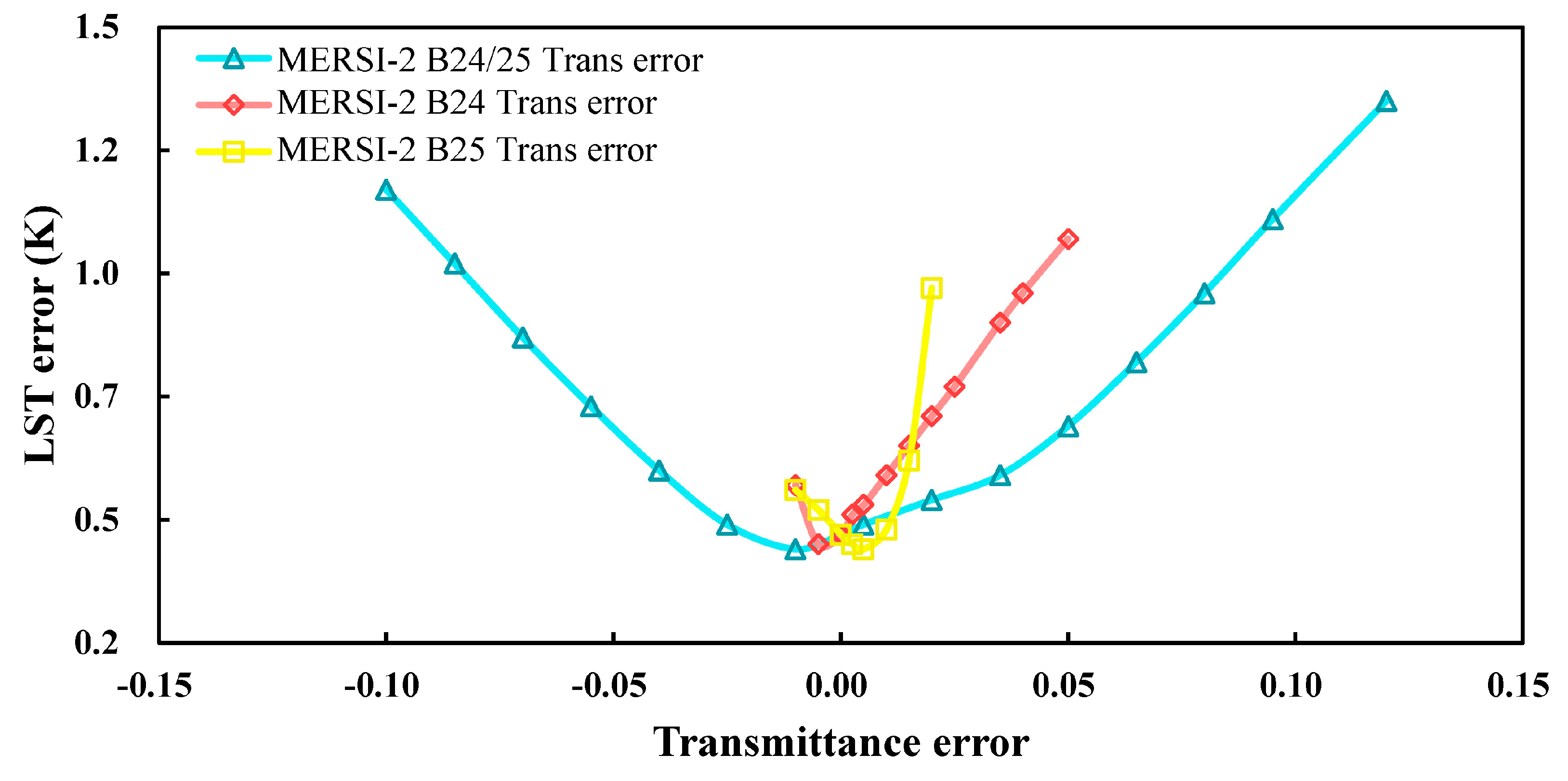
To further analyze the sensitivity of atmospheric transmittance, we conducted a separate study on atmospheric transmittance, as shown in
Figure 17. When we simultaneously change the transmittance error (−0.1–0.12) of MERSI-2 Bands 24 and 25 at the same ratio, the LST error ranges from 0.39–1.3 K. When the transmittance error ranges from −0.025–0.02, the LST error is less than 0.5 K. When the transmittance error of MERSI-2 Band 24 remains unchanged, and the transmittance error (−0.01–0.02) of MERSI-2 Band 25 is changed, the LST error ranges from 0.39–0.92 K. Similarly, when we change only the transmittance error (−0.01–0.05) of MERSI-2 Band 24, the corresponding LST error ranges from 0.40–1.02 K. In general, the algorithm is sensitive to the atmospheric transmittance relative to the sensitivity of WVC. The algorithm is not sensitive to WVC, which proves that it is feasible to use the WVC to estimate the atmospheric transmittance and subsequently retrieve the LST. The introduction of WVC will greatly improve the applicability of the algorithm, and in future research, we can use prior knowledge of the sensitivity analysis to further improve the accuracy of the LST retrieval.
5.3. Sensitivity Analysis of Land Surface Emissivity
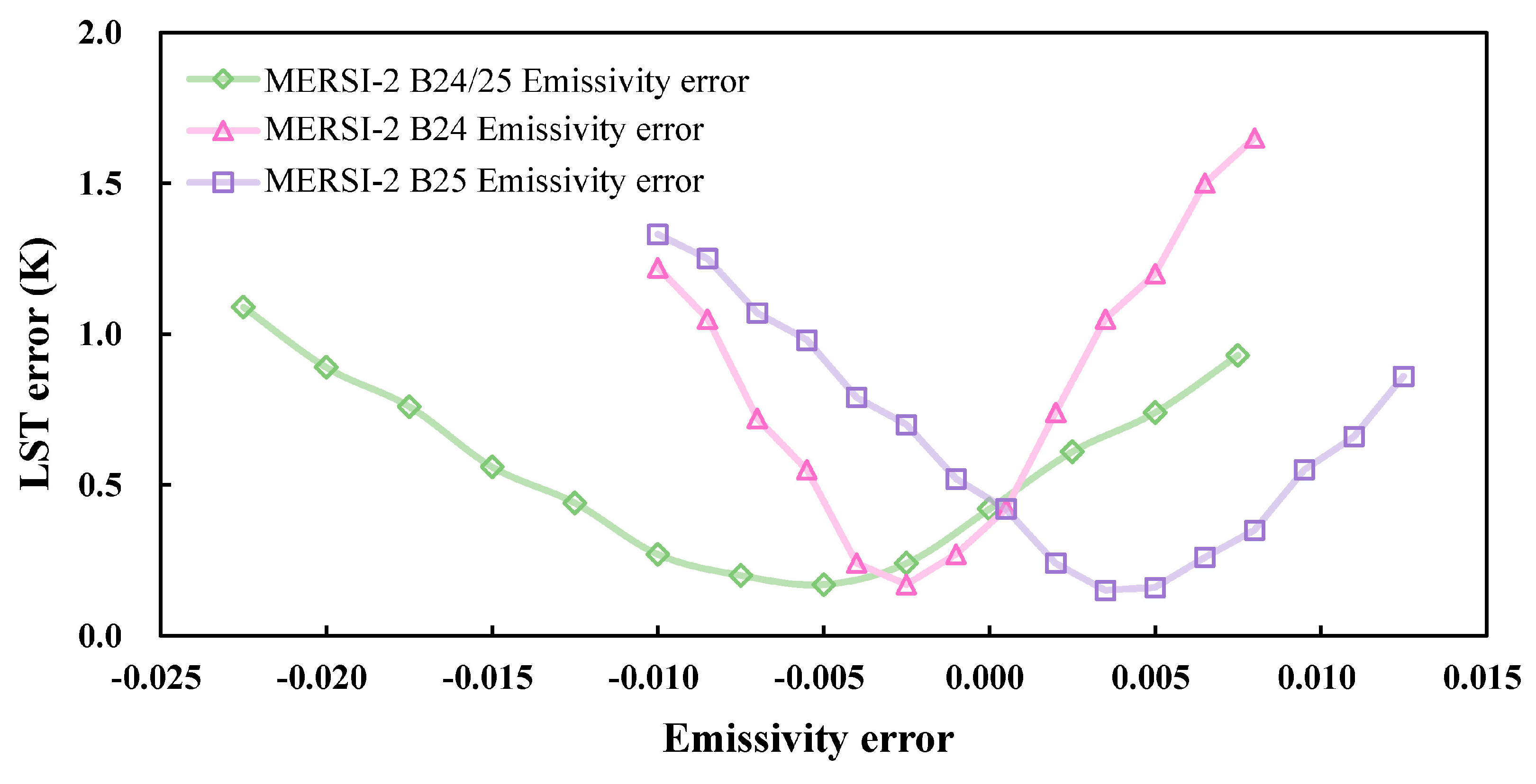
The change in emissivity is very important for the retrieval accuracy of the algorithm, and the sensitivity of our algorithm to emissivity was also analyzed, as shown in
Figure 18. When we simultaneously change the emissivity error (−0.023–0.008) of MERSI-2 Bands 24 and 25, the corresponding LST error ranges from 0.17–1.09 K; when the emissivity error ranges from −0.013–0, the LST error is less than 0.5 K. When we keep the emissivity error of MERSI-2 Band 24 unchanged, only the transmittance error (−0.01–0.013) of MERSI-2 Band 25 changes, and the corresponding LST error ranges from 0.15–1.33 K. Similarly, when we change only the transmittance error (−0.01–0.008) of MERSI-2 Band 24, the corresponding LST error ranges from 0.17–1.65 K. Through statistical analysis, we found that the emissivities of most features of MERSI-2 Bands 24 and 25 (10.30–11.30 μm and 11.50–12.50 μm) are higher than 0.97, and the degree of change is very small. Therefore, the algorithm is proven to not be sensitive to land surface emissivity.
The above analysis indicates that when the WVC and land surface emission error are within a certain range, the change in the surface temperature inversion error is within the acceptable range, which shows that the algorithm proposed in this study has good applicability. Furthermore,
Figure 16 and
Figure 18 show that the land surface emissivity is more sensitive to the estimation of the LST by the SW algorithm than to the WVC. Based on the dynamic changes in NDVI, we determined the land surface emission rate of MERSI-2 data in real time, overcoming the previous limitation that the emission rate did not change over time when land surface classification data were used. Moreover, we consider that at the spatial resolution of 1 km, the visible light bands can be used to divide the features in the image into soil, vegetation, and water. The NDVI is used to determine the proportions of the major land surface types in the mixed pixels. Thus, the land surface emissivity values corresponding to the pure pixels in the image and the mixed pixels are calculated, and finally, the estimation of the land emissivity is accurate at the subpixel level. In fact, in addition to the type of land surface, the land surface emissivity is also affected by land surface fluctuations (especially in mountainous areas) and is related to the geometry of different vegetation types and the location of vegetation in the pixels. Therefore, in future research, we need to pay more attention to the retrieval of the LST of heterogeneous pixel components to continuously improve the retrieval accuracy of LST.
6. Conclusions
Some deviations exist in TIR band radiance of MERSI-2; therefore, a cross-calibration model was built in this study that fully utilizes MODIS data. Without cross-validation, LST retrievals are nearly impossible. Therefore, a method for retrieving LST using the SW algorithm was proposed after BT cross-calibration, with the aim of providing support for the development of an LST product algorithm. Three methods were used to evaluate the accuracies of the retrieval results and algorithms. Moreover, we performed a detailed analysis of the main parameters that influence the algorithm, which are the WVC, transmittance, and emissivity, and finally, we proved that the algorithm has good applicability. The main conclusions are as follows:
(1) Cross-validation is of great significance for the study of LST retrievals. After cross-calibration of the MERSI-2 BT, the scaled value was basically consistent with the actual value, which was not the case for the uncalibrated value. To analyze a practical example, we used the cross-calibrated BT to retrieve the LST of the Bohai Sea area.
(2) In the LST retrieval stage, according to the characteristics of the NIR bands, we can retrieve the WVC and then calculate the atmospheric transmittance from the WVC of each pixel in the image. The land surface emissivity is estimated by the NDVI-based threshold method so that the main parameters for retrieving LST from the same image are acquired. Taking the Bohai Sea area as the research area, we used three methods to validate our algorithm. The results show that the average accuracy of the algorithm is 0.42 K when standard atmospheric simulation data are used, and the RMS is 0.19. When our retrieval results are compared with the MODIS LST product, the LST trends of MERSI-2 and MODIS are basically the same, while the average LST error is 1.37 K, and the RMS is 1.17. When our retrieval results are compared with ground-measured data, the evaluation results show that the accuracy of the SW algorithm is 1.23 K, and the RMS is 0.46. In general, the accuracy of the algorithm is relatively high, but the algorithm requires further improvement in subsequent research.
(3) After sensitivity analysis of the main parameters that affect the accuracy of the algorithm, namely, WVC, transmittance, and emissivity, the results show that the algorithm is not sensitive to the WVC and emissivity but is sensitive to transmittance. However, the feasibility of estimating transmittance from WVC is proven. Within a the reasonable interval (−13–13%) of the WVC and when the WVC error is between −20% and 100%, the average transmittance error of MERSI-2 Bands 24 and 25 is between 0 and 0.2, and at this time, the average LST errors are small (all less than 0.5 K), and the trends are stable; that is, the algorithm is not sensitive to WVC. Within a reasonable interval of emissivity change retrievals (generally higher than 0.97), when we change the emissivity error (−0.023–0.008) of MERSI-2 Bands 24 and 25, we can obtain an LST error range of 0.17–1.09 K, which also shows that our algorithm is not sensitive to emissivity. Compared with the interval of error variations for the WVC, our algorithm is slightly sensitive to atmospheric transmittance because when the MERSI-2 Bands 24 and 25 transmittance errors (−0.1–0.12) are changed simultaneously, the LST errors are 0.39–1.3 K. In general, the algorithm for estimating transmittance from atmospheric WVC to retrieve the LST has good applicability.
