Article

Precise Crop Classification Using Spectral-Spatial-Location Fusion Based on Conditional Random Fields for UAV-Borne Hyperspectral Remote Sensing Imagery

1
Faculty of Resources and Environmental Science, Hubei University, Wuhan 430062, China
2
Hubei Key Laboratory of Regional Development and Environmental Response, Hubei University, Wuhan 430062, China
*
Author to whom correspondence should be addressed.
Remote Sens. 2019, 11(17), 2011; https://doi.org/10.3390/rs11172011
Submission received: 21 June 2019 / Revised: 20 August 2019 / Accepted: 23 August 2019 / Published: 27 August 2019

Abstract

:
The precise classification of crop types is an important basis of agricultural monitoring and crop protection. With the rapid development of unmanned aerial vehicle (UAV) technology, UAV-borne hyperspectral remote sensing imagery with high spatial resolution has become the ideal data source for the precise classification of crops. For precise classification of crops with a wide variety of classes and varied spectra, the traditional spectral-based classification method has difficulty in mining large-scale spatial information and maintaining the detailed features of the classes. Therefore, a precise crop classification method using spectral-spatial-location fusion based on conditional random fields (SSLF-CRF) for UAV-borne hyperspectral remote sensing imagery is proposed in this paper. The proposed method integrates the spectral information, the spatial context, the spatial features, and the spatial location information in the conditional random field model by the probabilistic potentials, providing complementary information for the crop discrimination from different perspectives. The experimental results obtained with two UAV-borne high spatial resolution hyperspectral images confirm that the proposed method can solve the problems of large-scale spatial information modeling and spectral variability, improving the classification accuracy for each crop type. This method has important significance for the precise classification of crops in hyperspectral remote sensing imagery.

Graphical Abstract

1. Introduction

China is one of the most populous countries in the world. With the rapid development of urbanization, crop protection in China is becoming more and more important [1,2]. Managing and monitoring agricultural areas and crop types in a timely manner is the basic requirement for ensuring food security [3]. The traditional methods of obtaining crop planting information include field surveys and statistical sampling. Although these methods are both accurate and objective, they have shortcomings in large-scale implementation and do not provide accurate spatial distribution information for crop areas [4]. With the development of remote sensing technology, the use of remote sensing imagery to classify crops is an effective way to monitor the spatial distribution of agriculture and obtain basic data for crop growth monitoring and yield forecasting [5,6].
Most Chinese agricultural systems are dominated by smallholder family farming, which provides 70–80% of Chinese food sources [7]. These smallholder family farms are characterized by a small scale (less than 2 hectares, blurred boundaries), large distribution areas, mixed planting, etc. [8], meaning that traditional satellite-based multispectral remote sensing images and hyperspectral remote sensing images are unable to provide a sufficient data resolution for precision agriculture applications. However, the technology of unmanned aerial vehicles (UAVs) and light-weight sensors has provided an effective boost to the development of precision agriculture [9].
Compared with satellite or airborne data acquisitions, UAVs have a lower operating cost [10,11], are capable of more flexible operation [10,12], and allow more flexible flight route design [13]. UAVs can realize the rapid monitoring of crops and natural resources under custom temporal and spatial scales, and are now being widely used in the fields of precision agriculture, land-cover mapping [13], vegetation studies, environmental studies, and disaster monitoring [14]. Pádua et al. [15] used multi-temporal RGB images obtained by UAV to monitor grapevine growth; Zhou et al. [16] used two cameras in different spectral ranges installed on a UAV to obtain multi-temporal images to predict rice yield; and Marcial-Pablo et al. [17] used RGB and UAV-based multispectral images to estimate the vegetation fraction of corn. Hyperspectral sensors can be installed on UAVs to obtain hyperspectral remote sensing images with a high spatial resolution. Therefore, more and more spectral information and richer spatial information can be obtained in these images. At the same time, however, the simple use of spectral classification alone can no longer be applied to the classification of high spatial resolution hyperspectral data, and more spatial features need to be extracted for the precise classification of crops.
The random field model is one of the research hotspots of classification methods based on spatial context information, and it can construct scale-independent contextual information in a unified probability framework. The Markov random field (MRF) model is a typical random field model that can model the contextual information of the classification label, but it assumes that the observation information is conditionally independent, which limits the flexibility of spatial information utilization [18]. The conditional random field (CRF) model has flexibility of modeling, which overcomes the shortcomings of the MRF model and allows the posterior probability of given observation data to be directly modeled [19]. In the CRF model, the local potential function defines the relationship between random variables in the clique. Based on the different types of cliques, the potential function can be divided into unary potential, pairwise potential, and higher-order potential functions. The pairwise CRF model has been successfully applied to remote sensing processing and classification [20,21,22,23,24,25]. For example, the support vector conditional random field classifier incorporating a Mahalanobis distance boundary constraint (SVRFMC) can not only avoid the explicit modeling of observed data, but can also undertake appropriate smoothing with the consideration of contextual information by integrating SVM and a Mahalanobis distance boundary constraint [21]. The detail-preserving smoothing classifier based on conditional random fields (DPSCRF) considers the interaction of segmentation and classification in the CRF model, and adds spatial context information by segmentation [24]. For spatial–spectral fusion based on conditional random fields for the fine classification of crops in UAV-borne hyperspectral remote sensing imagery (SSF-CRF), the spatial and spectral features of the high spatial resolution hyperspectral data are fused by combining suitable potential functions in a pairwise conditional random field model to precisely classify crops [25]. However, these pairwise CRF models have difficulty in directly modeling large-scale spatial interaction information, resulting in the model often producing local over-smoothing and spectral variability in classification problems [23]. In the face of the problem of precise classification of crops with a wide variety and varied spectra, the traditional potential functions have difficulty in maintaining the details of the features in the classification, and will affect the accuracy of some classes due to the confusion with other classes.
Therefore, in this paper, in view of the problems of local over-smoothing and spectral variability faced by the CRF model in the precise classification of crops based on high-resolution hyperspectral remote sensing images, we propose a method for the precise classification of crops using spectral-spatial-location fusion based on conditional random fields (SSLF-CRF) for UAV-borne hyperspectral remote sensing imagery. The proposed method is further deepened on the basis of SSF-CRF, which constructs a unary potential function that combines spectral and spatial feature information, a pairwise potential function of the spatial context information, and a higher-order potential function of the spatial location information. In the method of SSLF-CRF, the spectral information provides the most basic judgment for classification, based on the spectral diversity of different features; the spatial feature information offers more detailed information; the spatial context information uses the spatial relationship of neighboring pixels to spatially smooth and reduce noise; and the spatial location information provides complementary information for classification from the perspective of the non-local similarity of classes, which helps to distinguish similar land-cover types

2. Method

2.1. The SSLF-CRF Model

CRF is a probabilistic discriminant model. The maximum posterior probability P ( x | y ) distribution is directly modeled as a Gibbs distribution [26,27], under the condition of given observation data, avoiding modeling the probability distribution of observed variables and having more flexible contextual information modeling capabilities, as shown in Equation (1):
P ( x | y ) = 1 Z ( y ) exp { c C ψ c ( x c , y ) }
where the high spatial resolution hyperspectral remote sensing imagery is represented as y = { y 1 , y 2 , , y N } ; y i is the spectral vector of the pixel at image position i, where i V = { 1 , 2 , , N } and N is the total number of pixels in the observed data; x = { x 1 , x 2 , , x N } is the class labels of the whole image; x i ( i = 1 , 2 , N ) comes from the label set L = { 1 , 2 , , K } , where K is the number of classes; Z ( y ) = x exp { c C ψ c ( x c , y ) } is the normalization function; and ψ c ( x c , y ) is the potential function of clique c to model the relationship of the random variables, where C is the set of all the cliques, which represents a fully connected subgraph. Correspondingly, the Gibbs energy is as shown in Equation (2):
E ( x | y ) = log P ( x | y ) log Z = c C ψ c ( x c , y )
Based on the CRF model, the goal of image classification is to find the largest label image x by the Bayesian maximum a posteriori (MAP) rule, so that the posterior probability P ( x | y ) is the largest. Therefore, the MAP label XMAP of the random field can be expressed as:
X M A P = arg max P ( x | y ) X = arg min E ( x | y ) X
Therefore, in the classification problems of the CRF model, maximizing the posterior probability distribution P ( x | y ) is equivalent to minimizing the energy function E ( x | y ) . In the proposed method, a higher-order CRF model, with the ability to encode higher-order spatial information, is used to improve the classification performance. The higher-order CRF model can be written as:
E ( x | y ) = i V ψ i ( x i , y ) + i V , j N i ψ i j ( x i , x j , y ) + c C ψ c ( x c , y )
where ψ i ( x i , y ) is the unary potential function; and ψ i j ( x i , x j , y ) is the pairwise potential function, which is defined over the local neighborhood Ni of the site of i. C represents the set of higher-order cliques, and ψ c ( x c , y ) is the higher-order potential function defined over these cliques. In the proposed method, an eight-neighborhood system is used to encode the interactions of the neighboring variables. In view of the characteristics of high spatial resolution hyperspectral remote sensing imagery and the requirements for the precise classification of crops, the unary potential, the pairwise potential, and the higher-order potential are modeled on the basic framework shown in Equation (4).

2.1.1. Unary Potential

The unary potential function models the relationship between the label data and the observed data, and obtains the cost penalty of the specific labeled class by the class member probability of the corresponding pixel. Each pixel can be independently calculated using any discriminant classifier that gives the probability of the label, which is usually defined as:
ψ i ( x i , y ) = ln { P [ x i = l k | f i ( y ) ] }
where f is a feature mapping function that maps any arbitrary subset of a contiguous image cell to a feature vector, and f i ( y ) represents the feature vector at position i. P [ x i = l k | f i ( y ) ] is the probability of pixel i acquiring the label lk that is based on the feature vector. Since the support vector machine (SVM) classifier performs well in remote sensing image classification with a small number of training samples [28,29], we use the SVM classifier, with a radial basis function as the kernel type, to provide the discriminant information of the classes based on the spatial-spectral feature vector. In the proposed method, the two parameters C and γ are set to the default values.
(1) Spectral Characteristics
Hyperspectral remote sensing imagery usually contains tens or even hundreds of spectral bands, so the spectral values of adjacent bands in hyperspectral images usually have a strong correlation [30], which results in data redundancy and can generate a “dimension disaster” problem during classification [31]. Minimum noise fraction (MNF) rotation is a commonly used method for extracting spectral features, and it is both simple and easy to implement. After MNF transformation, the components are arranged according to the signal-to-noise ratio, where the information is mainly concentrated in the first component. As the components increase, the image quality gradually decreases. Studies have shown that, compared with the original high-dimensional image data and the feature image obtained by principal component analysis (PCA) transformation, the low-dimensional feature image obtained by MNF transformation can extract the spectral information more effectively [32]. Therefore, we choose this method to extract the spectral information of the high spatial resolution hyperspectral imagery.
(2) Spatial Feature Characteristics
(A) Texture Features
Hyperspectral remote sensing images not only have continuous and abundant spectral information, but also rich texture information. Texture is the visual effect caused by spatial variation in tonal quantity over relatively small areas, which has been widely used in remote sensing image processing [33,34,35,36]. A number of studies have demonstrated the efficiency of texture for improving land-cover classification accuracy [37,38]. The gray-level co-occurrence matrix (GLCM) is a commonly used method for extracting texture information with a better discriminative ability [39,40]. The principle is to establish a GLCM between two pixels in a certain positional relationship in the image and to extract the corresponding feature quantity from this matrix for the texture analysis.
If we let f ( x , y ) be a two-dimensional digital image of size M × N , and the gray level is Ng, then the GLCM satisfying a certain spatial relationship is:
P ( i , j ) = # { ( x 1 , y 1 ) , ( x 2 , y 2 ) M , N | f ( x 1 , y 1 ) = i , f ( x 2 , y 2 ) = j }
where # ( x ) is the number of elements in the set x, and P is the matrix of N g × N g . If the distance between ( x 1 , y 1 ) and ( x 2 , y 2 ) is d and the angle is θ, then the GLCM P ( i , j , d , θ ) of various spacings and angles is:
P ( i , j , d , θ ) = # { ( x 1 , y 1 ) , ( x 2 , y 2 ) M , N | f ( x 1 , y 1 ) = i , f ( x 2 , y 2 ) = j }
In this paper, we use the six texture metrics of homogeneity, angular second moment, contrast, dissimilarity, mean, and entropy:
H o m = i = 0 L 1 j = o L 1 p ( i , j ) 1 + ( i j ) 2
A S M = i = 0 L 1 j = 0 L 1 p ( i , j ) 2
C o n = n = 0 L 1 n 2 { i = 0 L 1 j = 0 L 1 p ( i , j ) } n = | i j |
D i s = i = 0 L 1 j = 0 L 1 | i j | p ( i , j )
M e a n = 1 n × n i j f ( i , j )
E n t = i = 0 L 1 j = 0 L 1 p ( i , j ) log 2 p ( i , j )
(B) Endmember Components
There are some mixed pixels in high spatial resolution hyperspectral images, which have a certain degree of influence on the classification. If a method of mixed pixel decomposition is used, the corresponding percentage of each class in the mixed pixel can be expressed, thereby obtaining an abundance image equal to the number of classes. The endmember is a physical quantity associated with a mixed pixel. It is the main parameter describing the linear mixed model, representing the characteristic feature with a relatively fixed spectrum. The endmember extraction can obtain more detailed information of the image. In the proposed method, the sequential maximum angle convex cone (SMACC) endmember model is used to extract the endmember spectra and the abundance image, to form the endmember component [41], which can be defined as:
H ( c , i ) = k N R ( c , k ) A ( k , j )
where H is the spectral endmember; c and i are the band index and the pixel index, respectively; k and j represent an index from 1 to the largest endmember; R is the matrix containing the endmember spectra; and A is the abundance matrix containing endmember j to endmember k in each pixel.
(C) Morphological Features
Mathematical morphology is an effective image feature extraction tool that describes the local characteristics of images. The basic morphological operations are corrosion, expansion, and opening and closing operations, which act on the image through a series of shape regions called structuring elements (SEs). The morphological opening and closing reconstructions are another common kind of operator, which have a better shape preservation ability than the classical morphological filters. Since the shape of the SEs used in the filtering is adaptive, with respect to the structures present in the image itself, it nominally introduces no shape noise [42,43], as shown in Figure 1. In the proposed method, we extract the spatial information of the images based on “opening reconstruction followed by closing reconstruction” (OFC), which can simultaneously smooth the bright and dark details of the structure while maintaining the overall feature stability and improving the consistency within the object area [44,45].
The OFC operator is a hybrid operation of opening by reconstruction (OBR) and closing by reconstruction (CBR), which can be defined as:
O F C S E ( f ) = γ R S E ( φ R S E ( f ) )
where φ R S E ( f ) indicates the closing reconstruction of image f , and γ R S E ( φ R S E ( f ) ) is the opening reconstruction of the closing reconstruction image.

2.1.2. Pairwise Potential

Based on the theory of spatial correlation, the pairwise potential function simulates the spatial context information between each pixel and its neighborhood by considering the spatial pattern prior knowledge of the land-cover classes, so that the spectral changes and noise can be mitigated. The pairwise potential function can model the spatial smoothing prior, and support adjacent pixels of the homogeneous region to obtain the same class label. In this paper, it is defined as shown in Equations (16) and (17) [46,47]:
ψ i j ( x i , x j , y ) = { 0     i f   x i = x j g i j ( y )    o t h e r w i s e
g i j = λ ( 1 + θ exp ( y i y j 2 ) / π i j 2 )
where ( i , j ) is the spatial position of the adjacent pixel, and g i j is the smoothing term associated with the data y , which is used to measure the difference between adjacent pixels. y i and y j are the spectral vectors representing the pixels of i and j . The parameters λ and θ are set to control the strength of the pairwise potential function, and π is twice the mean-square error between the spectral vectors of all the neighboring pixels in the image, i.e., 2 y i y j 2 , where . represents the mean operation. The pairwise potential function can encourage adjacent pixels to have the same class in the classification result, thereby enhancing the spatial correlation.

2.1.3. Higher-Order Potential

Location information in local areas can help to distinguish confusing classes and mitigate the effects of spectral variability. The higher-order potential function in the CRF model can capture richer spatial interactions, it can explicitly model the spatial location information by considering the non-local spatial interaction between the target pixel and the nearest-neighbor training data, and it can provide the complementary information of the feature class from the perspective of the non-local similarity of the class. It can be expressed as:
ψ c ( x c , y ) = ( i j 2 ) / δ s + y i y j 2 / δ r + K c
K c = ln ( k = 1 K exp ( i j 2 δ s ) exp ( y i y j 2 δ r ) )
j = arg min ( j i 2 ) j , j S k
k = arg min ( μ k y i 2 ) k , k M
( S , μ ) = arg min S , μ ( l = 1 , j S l M y j l μ l 2 ) , l = x i L
The higher-order cliques in the higher-order potential function consist of the target pixel i and the training data. y l is the training samples representing the class label l . The set S = { S 1 , S 2 , , S M } is a set of patterns formed by automatic clustering of training data y l , and μ is the center corresponding to each pattern. In the proposed method, an adaptive mean shift clustering algorithm is used to obtain M patterns of the same feature class. Each pattern of the same feature has similar spectral characteristics and is represented by its corresponding mode center. For the target pixel i to be calculated, a pattern that is most similar to each feature class can be obtained based on the spectral vector distance. In the modeled higher-order potential function, the candidate pixels of each class are searched by finding the nearest-neighboring pixel to the target pixel space position. Equation (18) calculates the higher-order potential function based on the distance using the candidate pixels of each feature class in the spatial location and the spectral domain, where the pixel at position i represents the target pixel to be calculated, and the pixel at j is the candidate pixel. δ s and δ r are two independent parameters, which are respectively set as the second smallest value of the spatial distances and spectral distances between the target pixel and the corresponding candidate pixel for each class. K c is a regularization constant.
Since the higher-order potential function can encode the spatial interaction between each target pixel and the training data, it can be transformed into a unary potential function for solving, and the higher-order potential function is re-described using the class member probability, as shown in Equation (23):
P H P ( x i = l k ) = exp ( ψ c ( x c , y ) ) = 1 exp ( K c ) exp ( i j 2 δ s ) exp ( y i y j 2 δ r )
After the higher-order potential function is transformed into the class member probability of the target pixel, the Gaussian decreasing function can be used to calculate the distance in the spatial location domain and in the spectral space. In this paper, the class membership probability obtained by the higher-order potential function is integrated with the unary potential function to effectively utilize the complementary advantages of the spectral and spatial position information, as shown in Equation (24):
ψ i ( x i ) = ln ( ( 1 β ) P ( x i = l k ) + β P H P ( x i = l k ) )
where β is a free parameter from 0 to 1 for balancing the spectral information and the spatial location information.

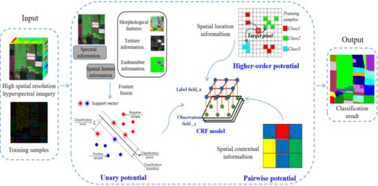
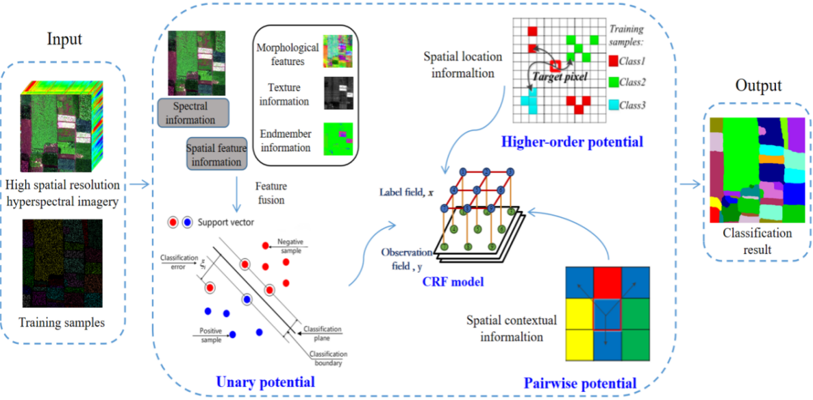
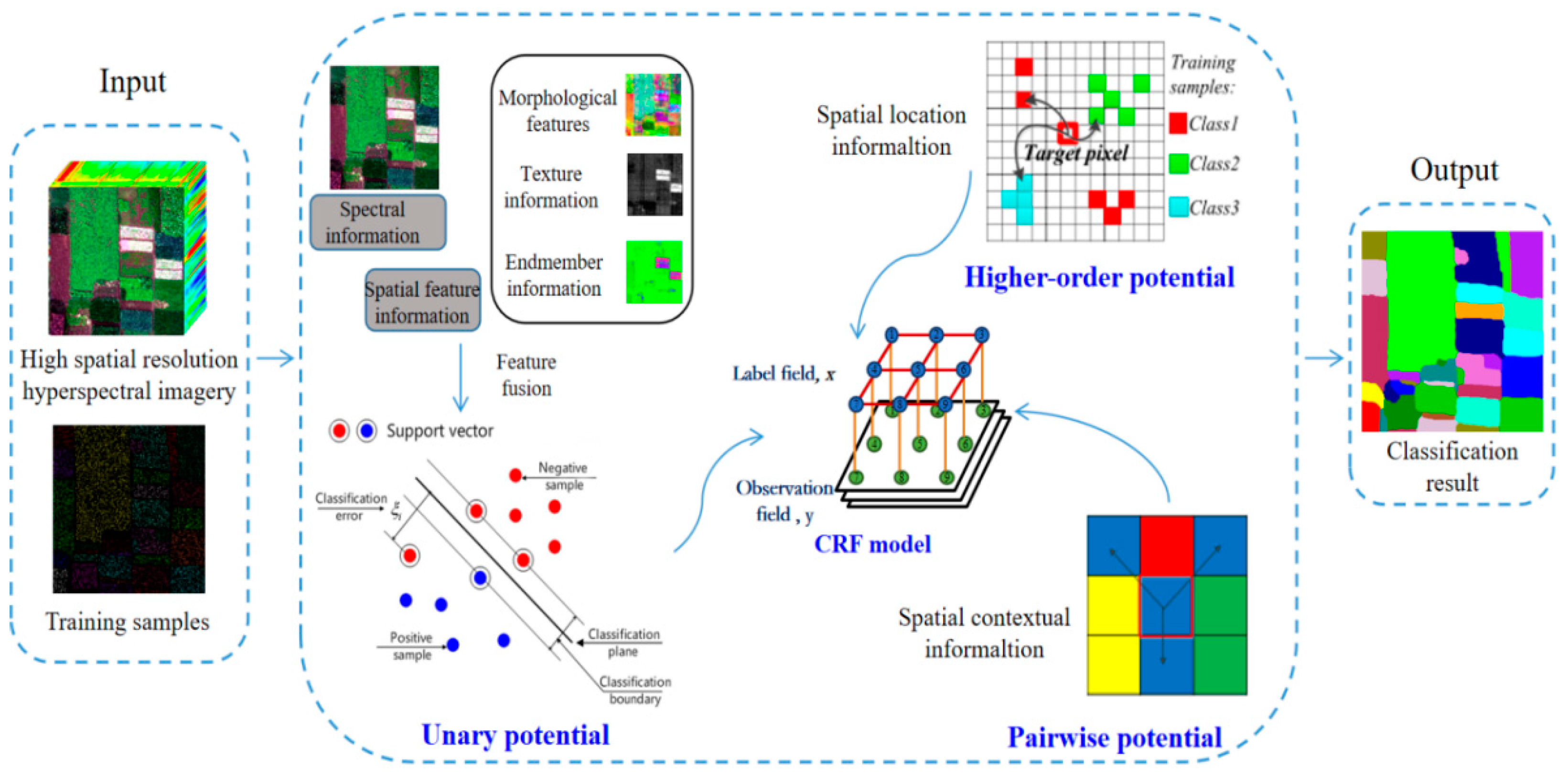
2.2. Algorithm Flowchart

The flowchart of the algorithm for precise crop classification using spectral-spatial-location fusion based on conditional random fields (SSLF-CRF) for UAV-borne hyperspectral remote sensing imagery is shown in Figure 2.
This method models the spectral information, the spatial feature information, the spatial context information, and the spatial location information through the unary potential, pairwise potential, and higher-order potential, respectively, which can integrate the complementary information from three different perspectives and make full use of the spatial information of the image, thereby improving the classification results. The SSLF-CRF method is described in detail as follows:
(1)
According to the characteristics of high spatial resolution hyperspectral remote sensing data obtained by UAV, the original image is subjected to MNF rotation. The noise covariance matrix in the principal component is used to separate and readjust the noise in the data, to minimize the variance of the transformed noise data and bands that are not relevant.
(2)
The unary potential function model the spectral and spatial feature information. The spectral information is the most basic information for judging the various land-cover classes, and the spatial feature information provides more details for the classification. Representative features are selected from the perspective of mathematical morphology, spatial texture, and mixed pixel decomposition, and then combined with the spectral information of each pixel to form a spectral-spatial fusion feature vector. The SVM classifier is used to model the relationship between the label and the spectral-spatial fusion feature vector, and the probability estimate of each pixel is calculated independently, based on the feature vector, according to the given label.
(3)
The spatial smoothing term simulates the spatial context information for each pixel and its corresponding neighborhood through the label field and observation field, which is modeled by the pairwise potential function. According to spatial correlation theory, the spatial smoothing term encourages the neighboring pixels of the homogeneous regions to share the same class label, and punishes the class discontinuity in the local regions.
(4)
Based on the characteristics of the similar spectral properties of the same feature class in a local region, the higher-order potential function is used to explicitly model the spatial location information by considering the training data of the target pixel closest to its spatial location, and it makes full use of the non-local similarity of the feature class to provide auxiliary information for the features that are difficult to distinguish. Differing from the spectral, spatial feature, and spatial contextual information, the spatial location information uses the regularity of the image to model the nonlocal similarity of the land-cover types through the location information.

3. Experimental Results
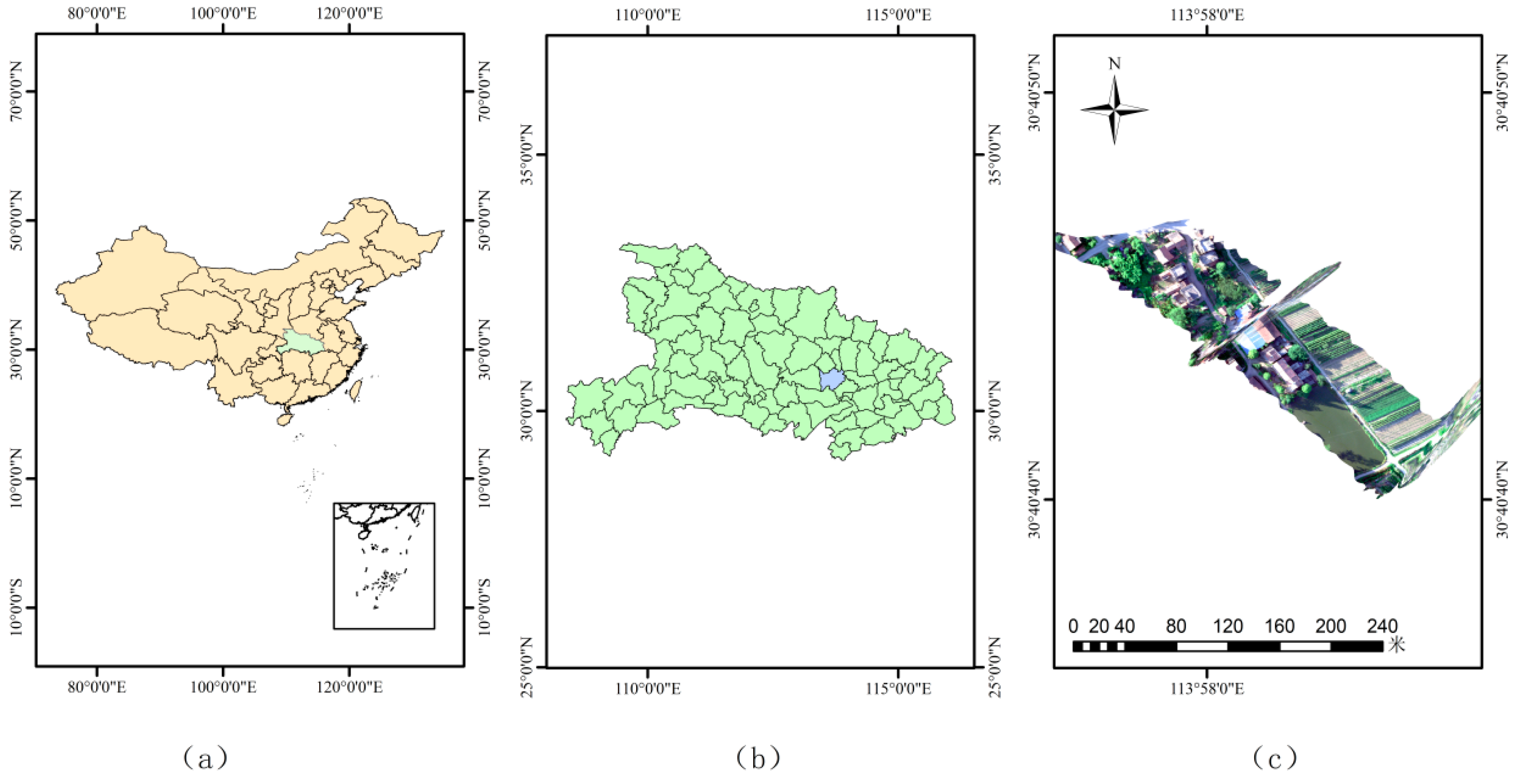
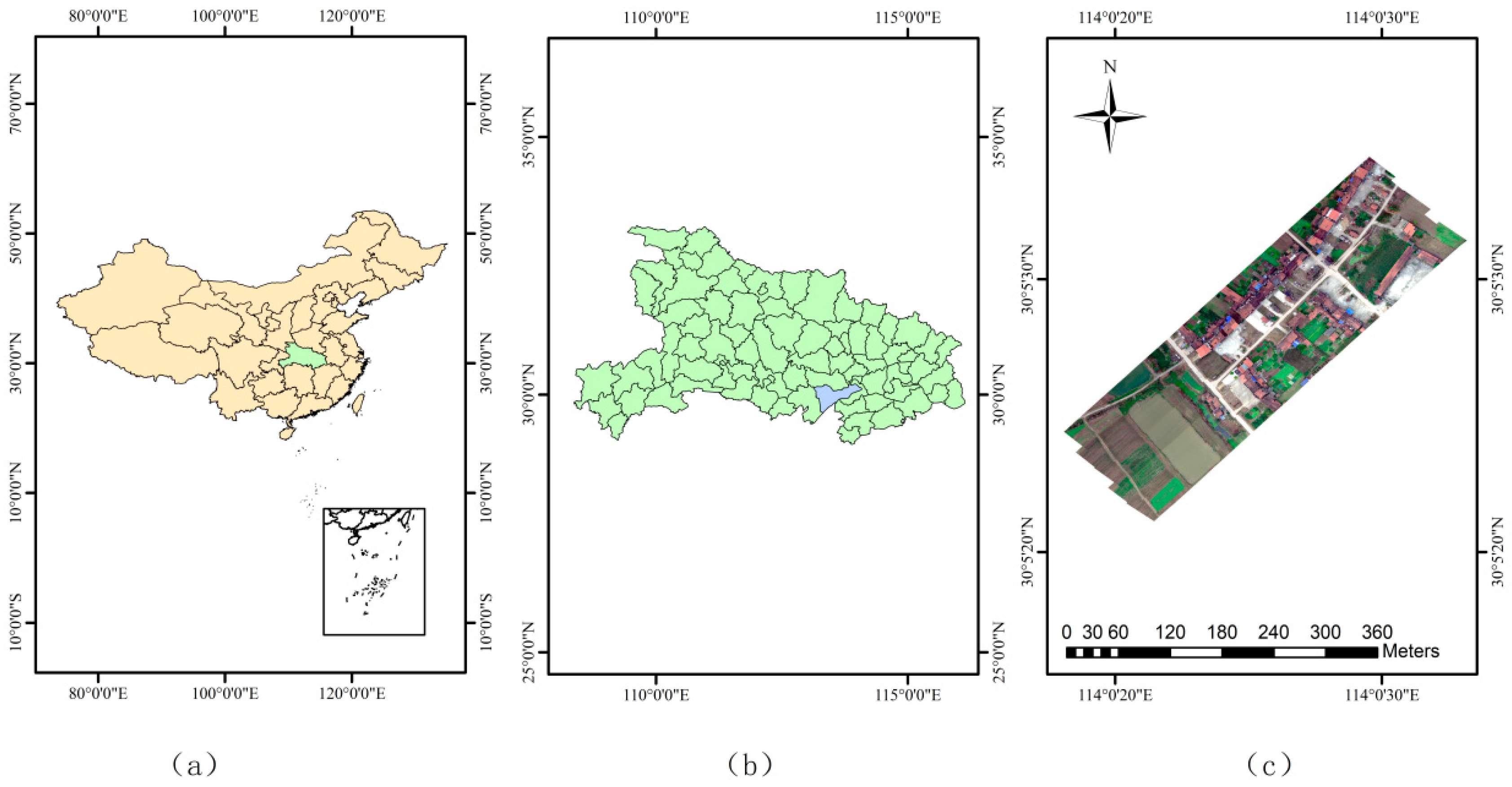
3.1. Study Areas

The two datasets used in the experiments cover the cities of Hanchuan (113°22′–113°57′E, 30°22′–30°51′N) and Honghu (113°07′–114°05′E, 29°39′–30°12′N) in Hubei Province, China (see Figure 3 and Figure 4).
Located in the central part of Hubei Province, China, the city of Hanchuan is situated on the lower reaches of the Han River and in the middle of the Jianghan Plain, where the terrain is flat and low-lying. The climate of this city is subtropical humid monsoon. A wide variety of crops are grown in the area, including rice, wheat, cotton, and rapeseed.
The city of Honghu is located in the south-central part of Hubei Province, in the middle and lower reaches of the Yangtze River, and in the southeast of Jianghan Plain. The terrain is higher in the north and south and is lower in the central part, forming a landform with a wide area and flat terrain. The climatic characteristics of the city of Honghu are similar to those of the city of Hanchuan, and both cities belong to the subtropical humid monsoon climate zone. The main crops of the Honghu area are cotton, rice, wheat, barley, broad beans, sorghum, and rapeseed.

3.2. Data Collection

The experimental data acquisition process consisted of two parts: (1) acquisition of aerial remote sensing images; and (2) acquisition of the ground truth. The drone model used for collecting the data was a DJI Matrice 600 Pro, and the hyperspectral imager was a Headwall Nano-Hyperspec hyperspectral imaging sensor manufactured by Headwall Photonics Inc. (Fitchburg, MA, USA) and provided by Xingbo Keyi Co., Ltd. (Guangzhou, China) ultra-micro airborne hyperspectral imaging spectrometer. This unit has a global positioning system/inertial measurement unit (GPS/IMU) navigation system and a complete data acquisition storage module. The integrated data acquisition system has Gig-E connection, which allows the data to be downloaded during flight. The synchronously acquired global positioning system/inertial navigation system (GPS/INS) data facilitate the subsequent geometric correction. Furthermore, the weight of the spectrometer is only 0.5 kg, which significantly reduces the burden on the UAV. The parameters of the Nano-Hyperspec imager are listed in Table 1.

3.3. Preprocessing of the UAV Images

Taking into account the hardware conditions and experimental requirements, the following pre-processing was performed on the high spatial resolution hyperspectral images acquired by the UAV: laboratory calibration, geometric correction, radiometric correction, and test sample production. In view of the low flight height of the drone, the complex atmospheric effects in flight could be ignored. The specific process of the preprocessing is described as follows:
(1)
The laboratory calibration of the sensor was the first step, converting the output signal of each sensor unit into an accurate radiance value.
(2)
The second step was geometric correction. The UAV integrates the sensors and the position and orientation system (POS) that combined with the differential GPS technology and Inertial Measurement Unit (IMU) technology, which can provide the position and attitude parameters of the sensor. For the geometric correction, the time standard of the POS data and hyperspectral image acquisition should be unified and corresponding. The correspondence between the image pixels and ground coordinates could thus be established by coordinate system transformation. Finally, the corrected pixels were resampled and the corrected image was reconstructed.
(3)
The third step was radiometric correction. We used a calibration blanket with a third-order reflectivity with reflectances of 11%, 32% and 56%, respectively. Before the UAV took off, the calibration blanket was placed in a suitable position in the study area to ensure that the study area and the calibration blanket appeared in the same image at the same time. Three sets of ROIs were selected in the three reflectance regions of the calibration blanket by means of ENVI, and the average radiation value of each group of ROIs was calculated. Finally, the standard reflectance of the calibration blanket and the radiation values could be linearly regressed in the IDL, according to Equation (25).
r e f l e c t a n c e = a · D N ( r a d i a n c e ) + b
(3)
The fourth step was test sample production. We obtained GPS linear feature information at where the data were acquired, and obtained ground marks with reference to the relative features synchronously, to generate the ground-truth data.

3.4. Experimental Description

In the experiments, the comparison algorithms were a pixel-based classification method, an object-oriented classification method, and random field based classification methods. The pixel-based classification method was the traditional SVM algorithm with a radial basis function as the kernel type. The object-oriented classification approach used a majority voting strategy for each segmentation region based on the same pixelwise SVM classification map. The segmentation was provided by mean shift segmentation (MS) [48]. The random field based methods were the Markovian support vector classifier (MSVC) [49], SVRFMC [21], DPSCRF [24], and SSF-CRF [25]. The MSVC algorithm integrates SVM into the MRF model, and obtains the final classification result through the iterated conditional modes (ICM) algorithm, using the Gaussian radial basis function and the Potts model as the kernel function and the local prior energy function, respectively. SVRFMC is a CRF classification algorithm based on Markov boundary constraints, where the spatial term is constrained by the Markov distance boundary, to maintain the spatial details of the classification results. DPSCRF considers the interaction of segmentation and classification in the CRF model, and adds large-scale spatial context information by segmentation. SSF-CRF fuses the spatial and spectral features of the high spatial resolution hyperspectral data by combining suitable potential functions in a pairwise conditional random field model.
In each experiment, three kinds of accuracies were used to assess the quantitative performance: the accuracy of each class, the overall accuracy (OA: the percentage of correctly classified pixels), and the Kappa coefficient (Kappa) [50]. For each algorithm, 1%, 3%, 5%, and 10% of the training samples were randomly selected to classify, and the remaining 99%, 97%, 95%, and 90% of the samples were used to verify the precision.

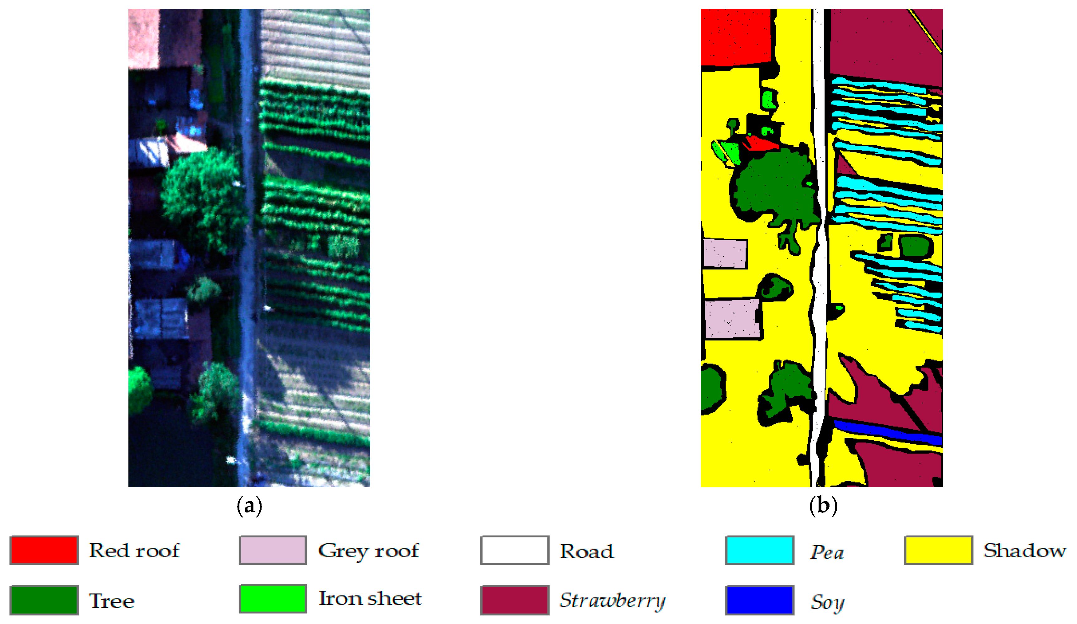
3.5. Experiment 1: Hanchuan Dataset

The dataset used in the first set of experiments was a UAV-borne high spatial resolution hyperspectral remote sensing image acquired over the city of Hanchuan, Hubei Province, China, in June 2016. The spatial resolution is 0.1 m. The image contains 303 × 600 pixels and 270 spectral channels, including nine land-cover classes: red roof, gray roof, tree, road, strawberry, pea, soy, shadow, and iron sheet. The true-color image is shown in Figure 5a and the corresponding ground-truth map is displayed in Figure 5b. Table 2 lists the number of training and test samples for each class at 1% training samples.
In the experiment with the Hanchuan dataset, the original image was reduced from 270 dimensions to 10 dimensions by MNF, according to the characteristics of the image. In order to introduce as little noise as possible, the most suitable spatial features were selected for the classification through a large number of experiments as follows: (1) the four endmembers of shadow, tree, strawberry, and red roof; (2) the four texture features of homogeneity, angular second moment, contrast, and mean were extracted with a window of 7 × 7; and (3) the morphological features were extracted with a disk-shaped SE with a size of 8. The parameters λ , θ , and β were set to 0.7, 2.4, and 0.4, to obtain the best results.
The experimental results corresponding to the different classification algorithms (SVM, MS, SVRFMC, DPSCRF, MSVC, SSF-CRF, and SSLF-CRF) are shown in Figure 6. Figure 6a is the classification result of SVM, which delivers a salt-and-pepper appearance because this algorithm does not consider the spatial information. Figure 6b–g are the results of the algorithms that consider the spatial context and spatial feature information, where the classification effects are smoother and the visual effects are better than those of the SVM algorithm. However, due to the influence of spectral variation, the different algorithms show different performances in terms of detail retention. For example, as shown in Figure 5a, the spectra of the iron sheet, gray roof, pea, tree, and soy classes have a certain similarity, so it is a challenging task to accurately distinguish these classes. In Figure 6b–e, the iron sheet is not easily identified, and for the most part is misclassified as gray roof and road, as shown by the red box in the figures. The features in the black box are pea, but this part was misclassified as tree or soy in most of the methods.
When compared with the result of SSF-CRF, the edge of this part in SSLF-CRF is the clearest. The features in the blue box are soy, but this part is mainly classified as tree by the methods of MS, SVRFMC, DPSCRF, and MSVC. In the proposed SSLF-CRF method, while alleviating the salt-and-pepper noise, the above misclassified classes can also be correctly identified. With the proposed method, most of the land-cover classes maintain a more complete boundary shape and useful feature details, with a better visual classification performance.
The quantitative accuracy evaluation for the different algorithms (SVM, MS, SVRFMC, DPSCRF, MSVC, SSF-CRF, and SSLF-CRF) is provided in Table 3. As can be seen from Table 3, when the training samples are 1%, the OA and Kappa values of the algorithms merging spatial and spectral information are improved, compared to the pixel classification method of SVM. In particular, since the SSLF-CRF method combines spatial context, spatial features, spatial location information, and spectral information, the accuracy is improved by about 10%, which indicates the importance of spatial information for improving the classification accuracy. For the misclassification of classes due to spectral variability, the advantages of the SSLF-CRF method are also fully reflected in the accuracy evaluation. For example, the highest precisions for road and gray roof in the other algorithms are 76.42% and 76.88%, respectively, but with the SSLF-CRF method, the precision reaches 82.57% and 82.27%, representing increases of about 6%. That is to say, this algorithm can effectively distinguish the easily confused land-cover classes caused by spectral variation.

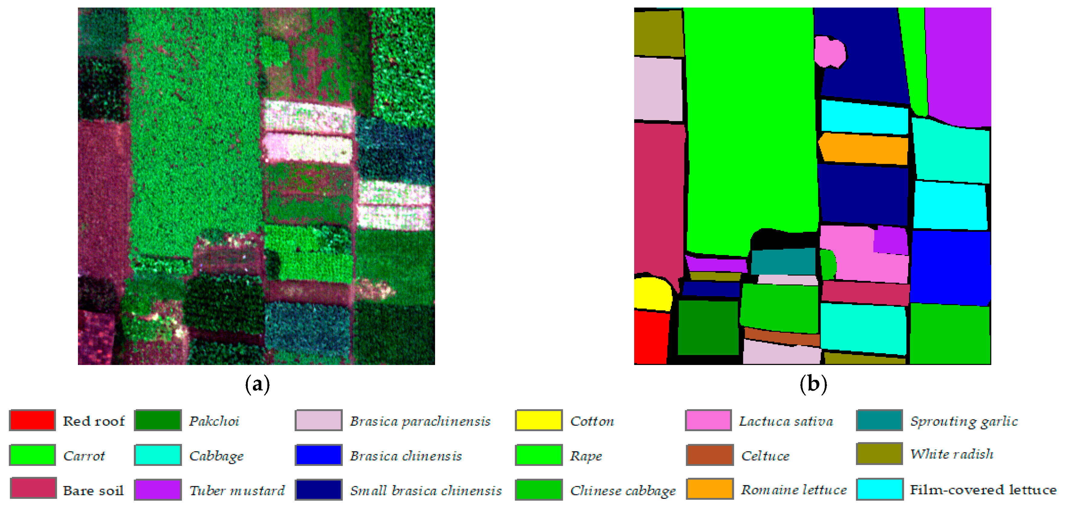
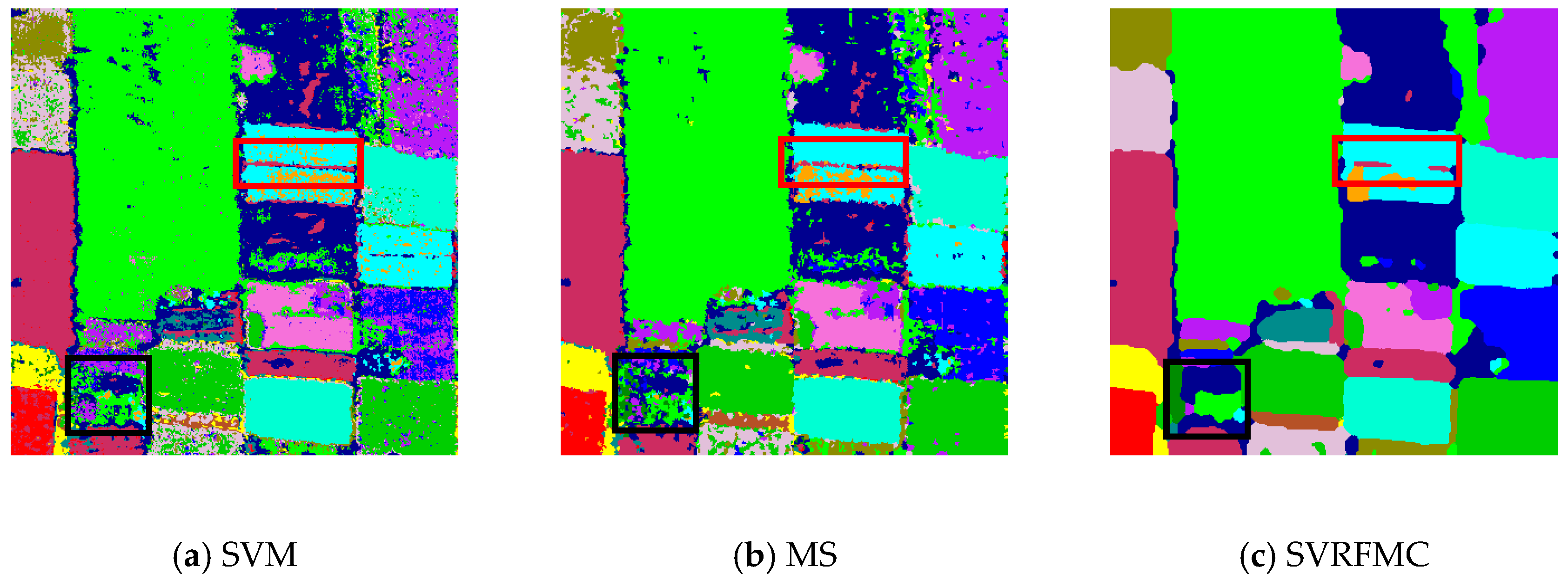
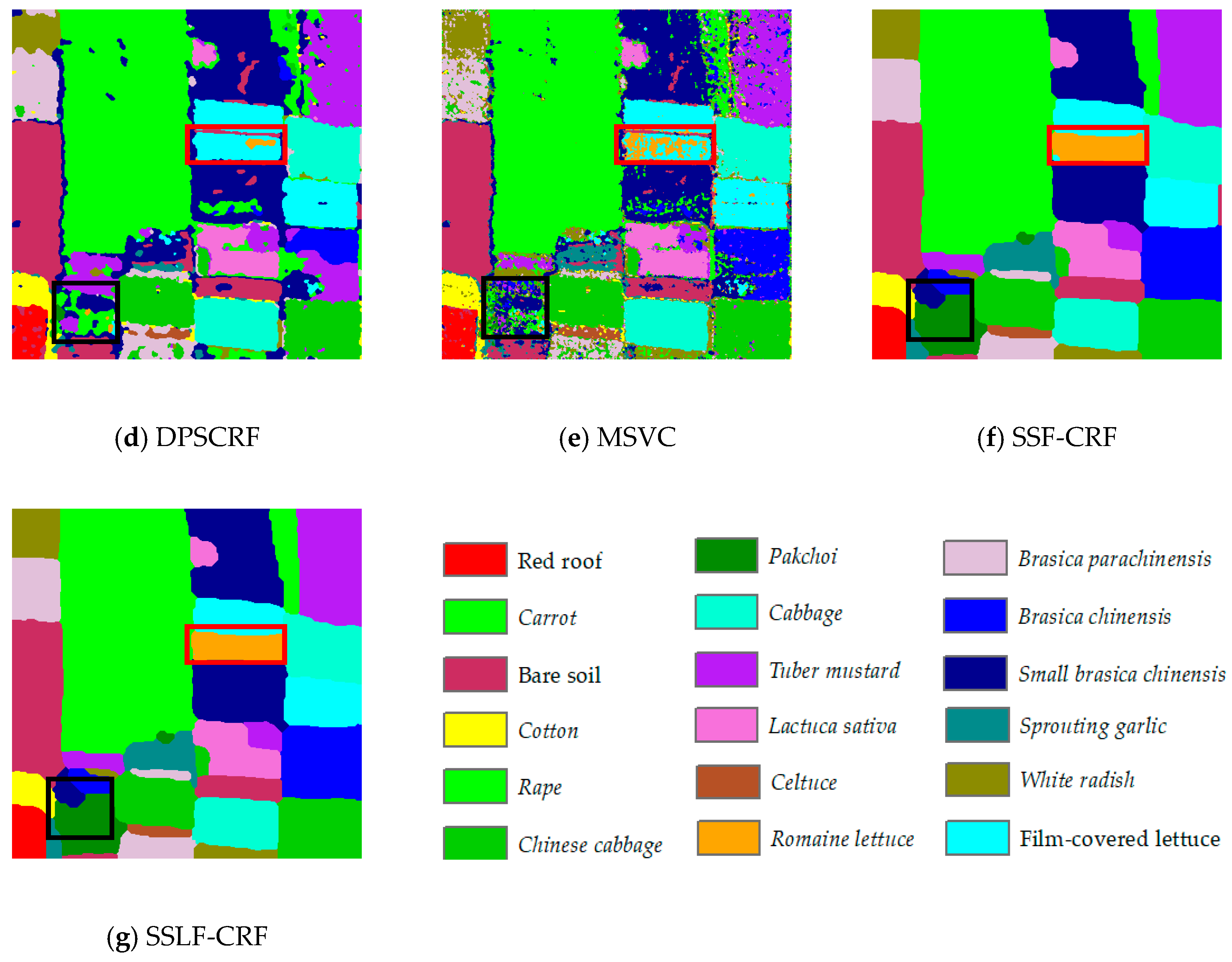
3.6. Experiment 2: Honghu Dataset

The second group of experiments used a UAV-borne hyperspectral remote sensing image with a 0.4-m spatial resolution acquired in Honghu City, Hubei Province, China, in November 2017. This image has a spatial dimension of 400 × 400 pixels and 270 spectral bands. In these experiments, 18 classes of interest were considered: red roof, bare soil, rape, cotton, Chinese cabbage, pakchoi, cabbage, tuber mustard, Brassica parachinensis, Brassica chinensis, small Brassica chinensis, Lactuca sativa, celtuce, film-covered lettuce, romaine lettuce, carrot, white radish, and spouting garlic. The overview of the area is shown in Figure 7a by the true-color image, and the corresponding reference ground truth is shown in Figure 7b. The numbers of randomly selected training and test samples for each class are listed in Table 4.
In order to introduce as little noise as possible while improving the experimental efficiency, the original data were reduced from 270 dimensions to 10 dimensions by MNF. The most suitable spatial features were selected for the classification through a large number of experiments as follows: (1) the four endmembers of bare soil, rape, and film-covered lettuce; (2) the four texture features of homogeneity, dissimilarity, entropy, and mean were extracted with a window of 7 × 7; and (3) the morphological features were extracted with a disk-shaped SE with a size of 8. The parameters λ , θ , and β were set to 0.4, 3.6, and 0.3, to obtain the best results.
For the experiments with the Honghu dataset, the experimental results corresponding to the different classification algorithms (SVM, MS, SVRFMC, DPSCRF, MSVC, SSF-CRF and SSLF-CRF) are shown in Figure 8a–g, respectively. As with the Hanchuan dataset, the classification result of the SVM algorithm in Figure 8a contains a large amount of salt-and-pepper noise. After considering the spatial context information, the classification effects of the various algorithms are greatly improved. As shown in Figure 8b–g, the salt-and-pepper noise is significantly reduced, and the boundaries of the various types of features are relatively complete. However, several types of crops with similar spectra in the Honghu dataset, such as romaine lettuce/film-covered lettuce and pakchoi/rape, are apparently misclassified due to the influence of spectral variation. As shown by the red box in Figure 8, the romaine lettuce is almost completely classified as film-covered lettuce in the classification results of the MS, SVRFMC, DPSCRF, and MSVC algorithms. The crop in the black box is pakchoi, but this is misclassified as rape, small Brassica chinensis, bare soil, and other features by the other algorithms. The SSLF-CRF algorithm considers the spatial features and the spatial location information, so for the above land-cover classes, not only are the types correctly identified, but the boundary shapes and details are also kept intact.
The accuracy evaluation for the different algorithms (SVM, MS, SVRFMC, DPSCRF, MSVC, SSF-CRF, and SSLF-CRF) is provided in Table 5. From the quantitative accuracy analysis, it can be seen that when the training samples are 1%, compared with the SVM pixel classification algorithm, the methods combining spatial information show an improvement in both OA and Kappa. For example, the accuracy of the object-oriented classification method of MS is improved by about 8%, and the results of the random field based methods of SVRFMC, DPSCRF, MSVC, SSF-CRF, and SSLF-CRF are improved by about 15%, 5%, 5%, 21% and 22%, respectively. Due to the consideration of the spatial location in SSLF-CRF, a better quantitative performance is shown in the classification accuracy. However, for those species with spectral variability, which are difficult to distinguish and easy to misclassify, the poor classification effect is reflected in the accuracy of each class. From Table 5, we can see that SSLF-CRF obtains a satisfactory result for each class, which indicates that the method not only considers the spectral information, but also combines the spatial features and spatial location information, effectively reducing the misclassification of the various classes.

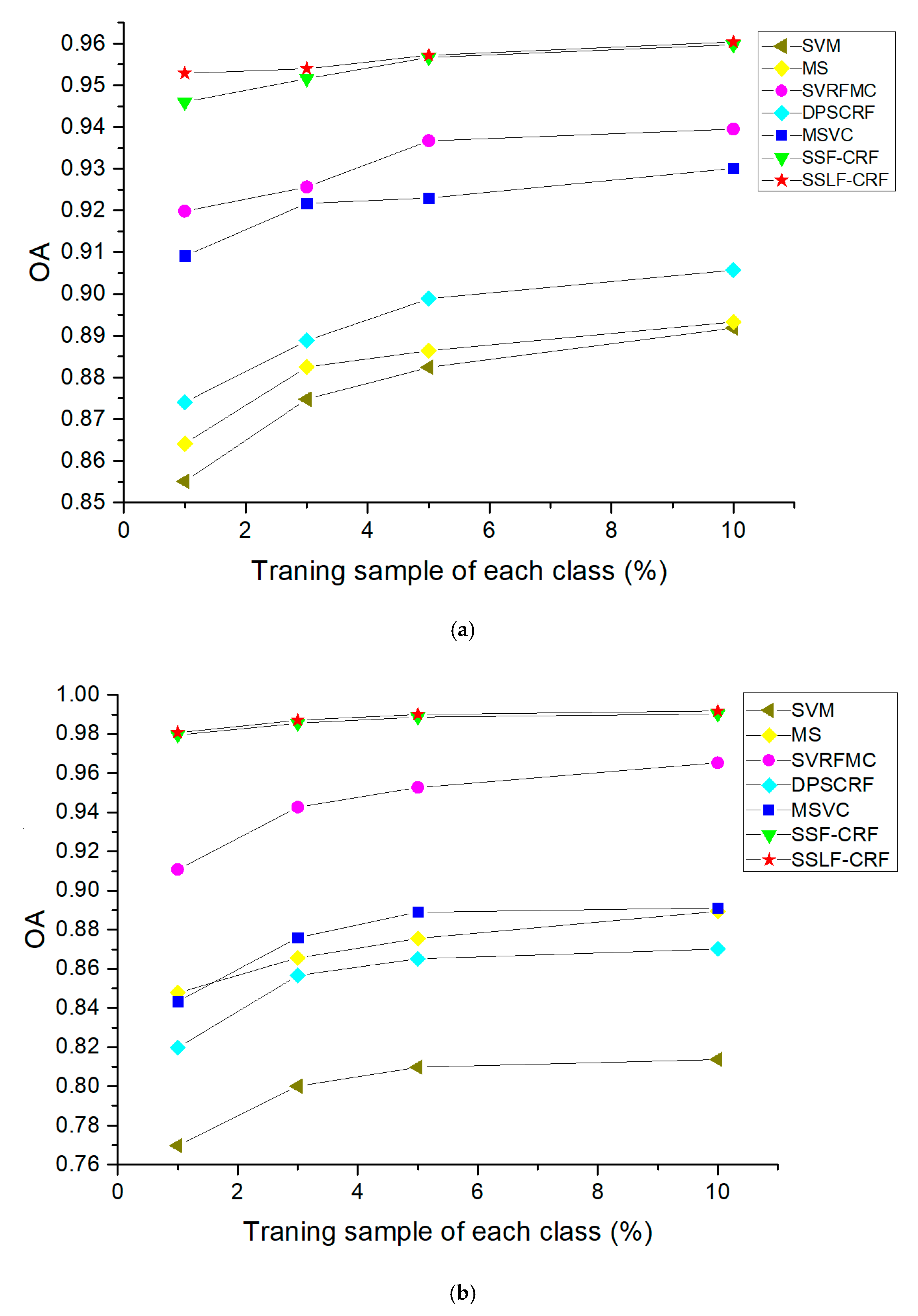
3.7. Sensitivity Analysis for the Training Sample Size

Training sample ratios of 1%, 3%, 5%, and 10% were used for each algorithm with each dataset to validate the SSLF-CRF method proposed in this paper. In all the experiments, we randomly selected 1%, 3%, 5%, and 10% training samples to validate each algorithm, and the remaining 99%, 97%, 95%, and 90% of the samples were used to evaluate the classification accuracy. The classification OAs for the different classification algorithms under different training sample sizes are shown in Figure 9.
We can see from Figure 9 that as the training samples increase, the accuracies of each algorithm increase significantly, for both datasets. However, given the different sizes of training samples, the performances of each algorithm in the two datasets are not exactly consistent, and are ranked as SSLF-CRF > SSF-CRF > SVRFMC > MSVC > DPSCRF > MS > SVM and SSLF-CRF > SSF-CRF > SVRFMC > MSVC > MS > DPSCRF > SVM, respectively. The object-oriented MS method performs better in the Honghu dataset than in the Hanchuan dataset.

4. Discussion

The important innovation of the proposed method is to integrate the spectral feature, spatial features, spatial context information and spatial location information of hyperspectral images by constructing higher-order potential function in the conditional random field model. The general crop classification methods are relatively simple, which may only use the above single or a few features, so that the image information cannot be fully utilized, and there is a certain room for improvement in classification accuracy. For UAV hyperspectral remote sensing image crop precise classification, spectral information provides the most basic information for their discrimination, based on the spectral differences of various land-cover classes; the spatial feature information provides more details for the classification from the perspective of mathematical morphology, texture and endmember components; the spatial context information takes into account the local spatial interaction of adjacent pixels, and provides spatial smoothing, which can effectively reduce the salt-and-pepper noise; the spatial location information fully exploits the spatial rule information of the image by considering non-local interactions of the same feature, providing auxiliary information for confusing classes. These information can offer complementary information for the discrimination of features from different angles, thus improving the classification effect to a certain extent and heightening the classification accuracy. Therefore, through constructing appropriate potential functions in the CRF model to fuse these features, this method can effectively improve the accuracy of crop precise classification of UAV hyperspectral remote sensing images, compared with the general classification methods.
In terms of sample selection, we randomly selected 1%, 3%, 5%, and 10% of training samples for classification. The remaining 99%, 97%, 95%, and 90% were used as test samples to verify classification accuracy. In the Hanchuan dataset, the accuracy of the proposed method increases with the training samples to a greater extent than with the Honghu dataset. This is because the Honghu dataset is more regular than the Hanchuan dataset. Therefore, even under 1% training samples, the proposed method can obtain a better classification accuracy, due to its strong ability to combine spatial information with spectral information.
In the UAV hyperspectral remote sensing image crop precise classification model of this paper, there are several aspects that can be optimized and further studied in the classification process. First of all, the extraction of spatial feature information is manually selected through a large number of experiments. This process can select the most suitable spatial features to participate in the classification, so that the classification effect is optimal, but it also takes a lot of time. So authors will perform automatic features extraction studies in the follow-up research to increase the efficiency of the method. Secondly, due to the limitation of the endurance of the drone, the experimental datasets obtained by us have small range, so this method is more advantageous when it is applied to small-and medium-scale crop classification applications. However, for common high resolution multi-spectral remote sensing images with rich spatial information, we can also combine them with hyperspectral remote sensing images to make them a data source with high spatial resolution and high spectral resolution. Therefore, it can be applied to the precise classification of crops in a wider range, and improve the applicability and application value of the research results.

5. Conclusions

With the rapid development of UAV technology, UAV-borne high spatial resolution hyperspectral data have become an ideal data source for the precise classification of crops. Based on the advantages of the high spatial resolution and high spectral resolution of this type of data, we have proposed a spatial-spectral-location fusion higher-order CRF precise crop classification method for UAV-borne hyperspectral remote sensing imagery. The proposed method integrates spectral and spatial feature, spatial context, and spatial location information in the higher-order CRF model, providing complementary information for the land-cover type discrimination from different perspectives, and mining the large-scale spatial local similarity of crops. It not only resolves the limitations of the pairwise CRF model in large-scale spatial context information modeling, but also greatly alleviates the problems of local over-smoothing and spectral variability encountered by the CRF model in the precise classification of crops based on high-resolution hyperspectral remote sensing imagery. The experiments on UAV-borne high spatial resolution hyperspectral remote sensing images of Hanchuan and Honghu (China), confirmed that the SSLF-CRF method shows an excellent classification performance, in terms of both qualitative and quantitative evaluations.

Author Contributions

L.W. and M.Y. were responsible for the overall design of the study. M.Y. performed all the experiments and drafted the manuscript. Y.L. and C.H. preprocessed the datasets. Z.Y., Y.Y. and R.L. contributed to designing the study. All authors read and approved the final manuscript.

Funding

This research was funded by the “National Key Research and Development Program of China” (2017YFB0504202), the “National Natural Science Foundation of China” (41622107), the “Central Government Guides Local Science and Technology Development Projects (2019ZYYD050)”, the “Special projects for technological innovation in Hubei” (2018ABA078), the “Open Fund of Key Laboratory of Ministry of Education for Spatial Data Mining and Information Sharing” (2018LSDMIS05), the “Open Fund of the State Laboratory of Information Engineering in Surveying, Mapping, and Remote Sensing, Wuhan University” (18R02) and the “Open fund of Key Laboratory of Agricultural Remote Sensing of the Ministry of Agriculture” (20170007).

Acknowledgments

The Intelligent Data Extraction and Remote Sensing Analysis Group of Wuhan University (RSIDEA) provided the datasets. The Remote Sensing Monitoring and Evaluation of Ecological Intelligence Group (RSMEEI) helped to process the datasets.

Conflicts of Interest

The authors declare no conflict of interest.

References

  1. Huang, J.; Ma, H.; Sedano, F.; Lewis, P.; Liang, S.; Wu, Q.; Su, W.; Zhang, X.; Zhu, D. Evaluation of regional estimates of winter wheat yield by assimilating three remotely sensed reflectance datasets into the coupled WOFOST–PROSAIL model. Eur. J. Agron. 2019, 102, 1–13. [Google Scholar] [CrossRef]
  2. Huang, J.; Sedano, F.; Huang, Y.; Ma, H.; Li, X.; Liang, S.; Tian, L.; Zhang, X.; Fan, J.; Wu, W. Assimilating a synthetic Kalman filter leaf area index series into the WOFOST model to improve regional winter wheat yield estimation. Agric. For. Meteorol. 2016, 216, 188–202. [Google Scholar] [CrossRef]
  3. Thenkabail, P.S. Global Croplands and their Importance for Water and Food Security in the Twenty-first Century: Towards an Ever Green Revolution that Combines a Second Green Revolution with a Blue Revolution. Remote Sens. 2010, 2, 2305–2312. [Google Scholar] [CrossRef] [Green Version]
  4. Shen, K.; He, H.; Meng, H.; Guannan, S. Review on Spatial Sampling Survey in Crop Area Estimation. Chin. J. Agric. Resour. Reg. Plan. 2012, 33, 11–16. [Google Scholar]
  5. Huang, J.; Tian, L.; Liang, S.; Ma, H.; Becker-Reshef, I.; Huang, Y.; Su, W.; Zhang, X.; Zhu, D.; Wu, W. Improving winter wheat yield estimation by assimilation of the leaf area index from Landsat TM and MODIS data into the WOFOST model. Agric. For. Meteorol. 2015, 204, 106–121. [Google Scholar] [CrossRef] [Green Version]
  6. Huang, J.; Ma, H.; Su, W.; Zhang, X.; Huang, Y.; Fan, J.; Wu, W. Jointly assimilating MODIS LAI and ET products into the SWAP model for winter wheat yield estimation. IEEE J. Sel. Top. Appl. Earth Obs. Remote Sens. 2015, 8, 4060–4071. [Google Scholar] [CrossRef]
  7. Lowder, S.K.; Skoet, J.; Raney, T. The number, size, and distribution of farms, smallholder farms, and family farms worldwide. World Dev. 2016, 87, 16–29. [Google Scholar] [CrossRef]
  8. Du, Z.; Yang, J.; Ou, C.; Zhang, T. Smallholder Crop Area Mapped with a Semantic Segmentation Deep Learning Method. Remote Sens. 2019, 11, 888. [Google Scholar] [CrossRef]
  9. Qi, J.; Sheng, H.; Yi, P.; Yan, G.; Ren, Z.; Xiang, W.; Yi, M.; Bo, D.; Jian, L. UAV-Based Biomass Estimation for Rice-Combining Spectral, TIN-Based Structural and Meteorological Features. Remote Sens. 2019, 11, 890. [Google Scholar] [Green Version]
  10. Colomina, I.; Molina, P. Unmanned aerial systems for photogrammetry and remote sensing: A review. ISPRS J. Photogramm. Remote Sens. 2014, 92, 79–97. [Google Scholar] [CrossRef] [Green Version]
  11. Hugenholtz, C.H.; Moorman, B.J.; Riddell, K.; Whitehead, K. Small unmanned aircraft systems for remote sensing and Earth science research. Eos Trans. Am. Geophys. Union 2012, 93, 236. [Google Scholar] [CrossRef]
  12. Zhong, Y.; Wang, X.; Xu, Y.; Wang, S.; Jia, T.; Hu, X.; Zhao, J.; Wei, L.; Zhang, L. Mini-UAV-Borne Hyperspectral Remote Sensing: From Observation and Processing to Applications. IEEE Trans. Geosci. Remote Sens. Mag. 2018, 6, 46–62. [Google Scholar] [CrossRef]
  13. Pajares, G. Overview and Current Status of Remote Sensing Applications Based on Unmanned Aerial Vehicles (UAVs). Photogramm. Eng. Remote Sens. 2015, 81, 281–330. [Google Scholar] [CrossRef] [Green Version]
  14. Shahbazi, M.; Théau, J.; Ménard, P. Recent applications of unmanned aerial imagery in natural resource management. GISci. Remote Sens. 2014, 51, 339–365. [Google Scholar] [CrossRef]
  15. Pádua, L.; Marques, P.; Hruška, J.; Adão, T.; Peres, E.; Morais, R.; Sousa, J. Multi-Temporal Vineyard Monitoring through UAV-Based RGB Imagery. Remote Sens. 2018, 10, 1907. [Google Scholar] [CrossRef]
  16. Zhou, X.; Zheng, H.; Xu, X.; He, J.; Ge, X.; Yao, X.; Cheng, T.; Zhu, Y.; Cao, W.; Tian, Y. Predicting grain yield in rice using multi-temporal vegetation indices from UAV-based multispectral and digital imagery. ISPRS J. Photogramm. Remote Sens. 2017, 130, 246–255. [Google Scholar] [CrossRef]
  17. Marcial-Pablo, M.d.J.; Gonzalez-Sanchez, A.; Jimenez-Jimenez, S.I.; Ontiveros-Capurata, R.E.; Ojeda-Bustamante, W. Estimation of vegetation fraction using RGB and multispectral images from UAV. Int. J. Remote Sens. 2019, 40, 420–438. [Google Scholar] [CrossRef]
  18. Tappen, M.F.; Liu, C.; Adelson, E.H.; Freeman, W.T. Learning Gaussian condition random fields for low-level vision. In Proceedings of the IEEE Conference on Computer Vision and Pattern Recognition, Minneapolis, MN, USA, 17–22 June 2007. [Google Scholar]
  19. Zhao, W.; Du, S.; Wang, Q.; Emery, W.J. Contextually guided very-high-resolution imagery classification with semantic segments. ISPRS J. Photogramm. Remote Sens. 2017, 132, 48–60. [Google Scholar] [CrossRef]
  20. Bai, J.; Xiang, S.; Pan, C. A Graph-Based Classification Method for Hyperspectral Images. IEEE Trans. Geosci. Remote Sens. 2013, 51, 803–817. [Google Scholar] [CrossRef]
  21. Zhong, Y.; Lin, X.; Zhang, L. A support vector conditional random fields classifier with a Mahalanobis distance boundary constraint for high spatial resolution remote sensing imagery. IEEE J. Sel. Top. Appl. Earth Obs. Remote Sens. 2014, 7, 1314–1330. [Google Scholar] [CrossRef]
  22. Zhong, Y.; Zhao, J.; Zhang, L. A Hybrid Object-Oriented Conditional Random Field Classification Framework for High Spatial Resolution Remote Sensing Imagery. IEEE Trans. Geosci. Remote Sens. 2014, 52, 7023–7037. [Google Scholar] [CrossRef]
  23. Zhong, P.; Wang, R. Modeling and Classifying Hyperspectral Imagery by CRFs with Sparse Higher Order Potentials. IEEE Trans. Geosci. Remote Sens. 2011, 49, 688–705. [Google Scholar] [CrossRef]
  24. Zhao, J.; Zhong, Y.; Zhang, L. Detail-preserving smoothing classifier based on conditional random fields for high spatial resolution remote sensing imagery. IEEE Trans. Geosci. Remote Sens. 2015, 53, 2440–2452. [Google Scholar] [CrossRef]
  25. Wei, L.; Yu, M.; Zhong, Y.; Zhao, J.; Liang, Y.; Hu, X. Spatial–spectral fusion based on conditional random fields for the fine classification of crops in UAV-borne hyperspectral remote sensing imagery. Remote Sens. 2019, 11, 780. [Google Scholar] [CrossRef]
  26. Lafferty, J.; Mccallum, A.; Pereira, F. Conditional random fields: Probabilistic models for segmenting and labeling sequence data. Proc. ICML 2001, 3, 282–289. [Google Scholar]
  27. Kumar, S.; Hebert, M. Discriminative random fields. Int. J. Comput. Vis. 2006, 68, 179–201. [Google Scholar] [CrossRef]
  28. Wu, T.; Lin, C.; Weng, R. Probability estimates for multi-class classification by pairwise coupling. J. Mach. Learn. Res. 2004, 5, 975–1005. [Google Scholar]
  29. Chang, C.; Lin, C. LIBSVM: A library for support vector machines. ACM Trans. Intell. Syst. Technol. 2011, 2, 1–27. [Google Scholar] [CrossRef]
  30. Li, W.; Feng, F.; Li, H.; Du, Q. Discriminant analysis-based dimension reduction for hyperspectral image classification: A survey of the most recent advances and an experimental comparison of different techniques. IEEE Geosci. Remote Sens. Mag. 2018, 6, 15–34. [Google Scholar] [CrossRef]
  31. Hughes, G. On the mean accuracy of statistical pattern recognizers. IEEE Trans. Inf. Theory 1968, 14, 55–63. [Google Scholar] [CrossRef]
  32. Simard, M.; Saatchi, S.; De Grandi, G. The use of decision tree and multiscale texture for classification of JERS-1 SAR data over tropical forest. IEEE Trans. Geosci. Remote Sens. 2000, 38, 2310–2321. [Google Scholar] [CrossRef] [Green Version]
  33. Anys, H.; He, D.C. Evaluation of textural and multipolarization radar features for crop classification. IEEE Trans. Geosci. Remote Sens. 1995, 33, 1170–1181. [Google Scholar] [CrossRef]
  34. Laliberte, A.S.; Rango, A. Texture and scale in object-based analysis of subdecimeter resolution Unmanned Aerial Vehicle (UAV) imagery. IEEE Trans. Geosci. Remote Sens. 2009, 47, 761–770. [Google Scholar] [CrossRef]
  35. Szantoi, Z.; Escobedo, F.; Abd-Elrahman, A.; Smith, S.; Pearlstine, L. Analyzing fine-scale wetland composition using high resolution imagery and texture features. Int. J. Appl. Earth Obs. 2013, 23, 204–212. [Google Scholar] [CrossRef]
  36. Aguera, F.; Aguilar, F.J.; Aguilar, M.A. Using texture analysis to improve per-pixel classification of very high resolution images for mapping plastic greenhouses. ISPRS J. Photogramm. Remote Sens. 2008, 63, 635–646. [Google Scholar] [CrossRef]
  37. Fu, Q.; Wu, B.; Wang, X.; Sun, Z. Building extraction and its height estimation over urban areas based on morphological building index. Remote Sens. Technol. Appl. 2015, 30, 148–154. [Google Scholar]
  38. Zhang, L.; Huang, X. Object-oriented subspace analysis for airborne hyperspectral remote sensing imagery. Neurocomputing 2010, 73, 927–936. [Google Scholar] [CrossRef]
  39. Maillard, P. Comparing texture analysis methods through classification. Photogramm. Eng. Remote Sens. 2003, 69, 357–367. [Google Scholar] [CrossRef]
  40. Beguet, B.; Chehata, N.; Boukir, S.; Guyon, D. Classification of forest structure using very high resolution Pleiades image texture. In Proceedings of the 2014 IEEE International Geoscience and Remote Sensing Symposium, Quebec City, QC, Canada, 13–18 July 2014; Volume 2014, pp. 2324–2327. [Google Scholar]
  41. Gruninger, J.; Ratkowski, A.; Hoke, M. The sequential maximum angle convex cone (SMACC) endmember model. Proc. SPIE 2004, 5425, 1–14. [Google Scholar]
  42. Pesaresi, M.; Benediktsson, J. A new approach for the Morphological Segmentation of high-resolution satellite imagery. IEEE Trans. Geosci. Remote Sens. 2001, 39, 309–320. [Google Scholar] [CrossRef]
  43. Benediktsson, J.; Pesaresi, M.; Arnason, K. Classification and feature extraction for remote sensing image from urban areas based on morphological transformations. IEEE Trans. Geosci. Remote Sens. 2003, 41, 1940–1949. [Google Scholar] [CrossRef]
  44. Yu, Q.; Gong, P.; Clinton, N.; Biging, G.; Kelly, M.; Schirokauer, D. Object-based detailed vegetation classification with airborne high spatial resolution remote sensing imagery. Photogramm. Eng. Remote Sens. 2006, 72, 799–811. [Google Scholar] [CrossRef]
  45. Hu, R.; Huang, X.; Huang, Y. An enhanced morphological building index for building extraction from high-resolution images. Acta Geod. Cartogr. Sin. 2014, 43, 514–520. [Google Scholar]
  46. Rother, C.; Kolmogorov, V.; Blake, A. ‘GrabCut’: Interactive foreground extraction using iterated graph cuts. ACM Trans. Graph. 2004, 23, 309–314. [Google Scholar] [CrossRef]
  47. Shotton, J.; Winn, J.; Rother, C.; Criminisi, A. Textonboost: Joint appearance, shape and context modeling for multi-class object recognition and segmentation. In Proceedings of the European Conference on Computer Vision, Amsterdam, The Netherlands, 8–16 October 2016; pp. 1–15. [Google Scholar]
  48. Qiong, J.; Landgrebe, D. Adaptive Bayesian contextual classification based on Markov random fields. IEEE Trans. Geosci. Remote Sens. 2003, 40, 2454–2463. [Google Scholar]
  49. Moser, G.; Serpico, S. Combining support vector machines and Markov random fields in an integrated framework for contextual image classification. IEEE Trans. Geosci. Remote Sens. 2013, 51, 2734–2752. [Google Scholar] [CrossRef]
  50. Richards, J.; Jia, X. Remote Sensing Digital Image Analysis: An Introduction, 4th ed.; Springer: New York, NY, USA, 2006. [Google Scholar]
Figure 1. Morphological reconstruction.
Remotesensing 11 02011 g001
Figure 2. Flowchart of the spectral-spatial-location fusion based on conditional random fields (SSFL-CRF) method.
Remotesensing 11 02011 g002
Figure 3. (a) The location of Hubei Province in China. (b) Administrative area map of the city of Hanchuan in Hubei Province. (c) The study site.
Remotesensing 11 02011 g003
Figure 4. (a) The location of Hubei Province in China. (b) Administrative area map of the city of Honghu in Hubei Province. (c) The study site.
Remotesensing 11 02011 g004
Figure 5. The Hanchuan dataset: (a) the true-color image; (b) the ground-truth map.
Remotesensing 11 02011 g005
Figure 6. Hanchuan dataset classification results: (a) support vector machine (SVM); (b) mean shift segmentation (MS); (c) support vector conditional random field classifier with a Mahalanobis distance boundary constraint (SVRFMC); (d) detail-preserving smoothing classifier based on conditional random fields (DPSCRF); (e) Markovian support vector classifier (MSVC); (f) spatial-spectral fusion based on conditional random fields (SSF-CRF); (g) spatial-spectral-location fusion based on conditional random fields (SSLF-CRF).
Remotesensing 11 02011 g006aRemotesensing 11 02011 g006b
Figure 7. The Honghu dataset: (a) the true-color image; (b) the ground-truth map.
Remotesensing 11 02011 g007
Figure 8. Honghu dataset classification results: (a) SVM; (b) MS; (c) SVRFMC; (d) DPSCRF; (e) MSVC; (f) SSF-CRF; (g) SSLF-CRF.
Remotesensing 11 02011 g008aRemotesensing 11 02011 g008b
Figure 9. Sensitivity analysis for the training sample size: (a) Hanchuan dataset; (b) Honghu dataset.
Remotesensing 11 02011 g009
Table 1. Nano-Hyperspec hyperspectral imaging sensor parameter information.
ClassParameterClassParameter
Wavelength range400–1000 nmField of view332216
Number of spectral channels270Storage480 GB
Lens focal length8 mm12 mm17 mmCamera typeCOMS
Operating temperature0~50℃Weight<0.6 kg (no lens)
Table 2. The training and test sample information for the Hanchuan dataset.
ClassTraining SamplesTest Samples
Red roof656525
Gray roof484766
Tree11711664
Road727138
Strawberry22622402
Pea11010937
Soy131322
Shadow76375609
Iron sheet101006
Table 3. The classification accuracies for the Hanchuan dataset.
ClassAccuracy (%)
SVMMSSVRFMCDPSCRFMSVCSSF-CRFSSLF-CRF
Red roof49.7248.8964.7549.9667.4382.1684.08
Tree67.3073.9592.4780.3884.3396.1297.12
Road65.0766.7774.9162.5875.3976.4282.57
Strawberry94.5595.3797.5496.8995.7498.0097.96
Pea64.1265.4979.5567.5178.3791.6692.90
Soy35.7829.9547.8113.9278.6789.2686.46
Shadow97.1997.4198.8497.5397.8398.0798.04
Gray roof53.9053.6774.2164.0672.0576.8882.27
Iron sheet42.2543.5422.0737.5743.8471.9769.88
OA85.5186.4191.9887.4090.9194.6095.29
Kappa0.77570.78900.87600.80430.86070.91770.9286
Table 4. The training and test sample information for the Honghu dataset.
ClassTraining SamplesTest SamplesClassTraining SamplesTest Samples
Red roof222182Brassica chinensis727181
Bare soil11811692Small Brassica chinensis15915769
Cotton141410Lactuca sativa525220
Rape37937541Celtuce10993
Chinese cabbage10710688Film-covered lettuce727191
Pakchoi404015Romaine lettuce302981
Cabbage10310204Carrot272766
Tuber mustard11411327White radish404042
Brassica parachinensis636240Spouting garlic202046
Table 5. The classification accuracies for the Honghu dataset.
ClassAccuracy (%)
SVMMSSVRFMCDPSCRFMSVCSSF-CRFSSLF-CRF
Red roof77.5993.7799.4086.1689.1898.4998.53
Bare soil93.8694.9798.1296.0794.0299.6699.82
Cotton83.5595.8998.5897.0991.7799.0199.08
Rape96.1998.9099.8098.1198.7399.9199.91
Chinese cabbage88.0094.6099.0093.8693.0499.4499.46
Pakchoi1.7914.9213.873.7610.7687.5087.90
Cabbage94.1397.2899.3097.2996.3299.5799.64
Tuber mustard63.1577.9690.1780.5270.8098.5498.75
Brassica parachinensis62.3672.7293.6983.5167.3297.6397.63
Brassica chinensis39.0266.0275.2034.3865.7698.4599.09
Small Brassica chinensis77.6882.6792.6884.3183.4694.9895.03
Lactuca sativa71.6376.3885.7574.7580.6597.1897.28
Celtuce42.3068.9887.5146.0271.4078.1578.45
Film-covered lettuce88.6596.3798.6997.6895.6199.7499.75
Romaine lettuce31.2336.3027.318.4543.1795.6496.04
Carrot34.8948.4882.4358.6860.4895.4196.28
White radish51.3172.6489.4659.3578.3392.4592.75
Sprouting garlic39.2061.2982.9421.8071.1697.2197.17
OA76.9784.7791.0881.9784.3297.9598.07
Kappa0.73670.82620.89850.79360.82170.97680.9782

