Abstract
Phytoplankton species composition research is key to understanding phytoplankton ecological and biogeochemical functions. Hyperspectral optical sensor technology allows us to obtain detailed information about phytoplankton species composition. In the present study, a transfer learning method to inverse phytoplankton species composition using in situ hyperspectral remote sensing reflectance and hyperspectral satellite imagery was presented. By transferring the general knowledge learned from the first few layers of a deep neural network (DNN) trained by a general simulation dataset, and updating the last few layers with an in situ dataset, the requirement for large numbers of in situ samples for training the DNN to predict phytoplankton species composition in natural waters was lowered. This method was established from in situ datasets and validated with datasets collected in different ocean regions in China with considerable accuracy (R2 = 0.88, mean absolute percentage error (MAPE) = 26.08%). Application of the method to Hyperspectral Imager for the Coastal Ocean (HICO) imagery showed that spatial distributions of dominant phytoplankton species and associated compositions could be derived. These results indicated the feasibility of species composition inversion from hyperspectral remote sensing, highlighting the advantages of transfer learning algorithms, which can bring broader application prospects for phytoplankton species composition and phytoplankton functional type research.
1. Introduction
Marine phytoplankton plays a crucial role in aquatic ecosystems [1]. It contributes to primary production, affects the abundance and diversity of marine organisms [2], and exerts influence on climate processes [3]. Therefore, a better understanding of phytoplankton greatly enhances our understanding of the carbon and nitrogen cycles in marine ecosystems [4,5]. Phytoplankton functional types are species groups with specific roles in biogeochemical cycles [6]. Because the physiological processes of different phytoplankton species and associated compositions are distinct from each other, each individual phytoplankton species and its associated composition information are fundamental to its functional type [7]. In addition, they are also indicative of variability in phytoplankton species diversity in the ocean [8]. With the development of satellite-based ocean color remote sensing, which provides the advantages of wide-range, long-term coverage, high efficiency, and low cost [9], phytoplankton species, composition, and related research from space have been carried out [10,11].
The inherent optical properties of different phytoplankton species or groups have been studied [12,13], and numerous efforts have been made to understand phytoplankton communities in aquatic systems with the advancement of ocean color remote sensing. Much research has been focused on the identification of specific phytoplankton species or groups under blooming conditions using ocean color satellites with a moderate spectral resolution [14,15,16]. Furthermore, discrimination of phytoplankton phyla in blooming conditions has been achieved based on differences in optical signals among different phytoplankton populations [17]. However, these endeavors are constrained to a limited type of phytoplankton species or groups because of the limitations in band settings for multi-spectral remote sensing. Moreover, some studies have been focused on Case 1 water with relatively simple optical properties where optically active constituents co-vary with chlorophyll concentration [18,19]; however, it is more challenging to invert phytoplankton species composition from current ocean color remote sensing data with moderate spectral resolution in optically complex waters. Comparatively, hyperspectral remote sensing presents a promising tool to resolve the spectral variability of phytoplankton species [20].
Several ocean color algorithms have also been proposed for phytoplankton information inversion in natural waters [21,22,23,24]. Among these efforts, a derivative spectroscopy/similarity index (SI) approach is the most common method for identifying dominant phytoplankton species or groups [25,26,27]. However, because SI-based approaches assign unknown spectra to the reference spectra that have the largest SI, only dominant species or groups can be identified, so it is difficult to determine phytoplankton species composition using this method, and the algorithm degradation for coastal waters with high suspended particulate matter (SPM) and colored dissolved organic matter (CDOM) is inevitable [28,29].
Regarding data acquisition, most studies on phytoplankton community structures are based on the high-performance liquid chromatography–chemical taxonomy (HPLC-Chemtax) method [30]. On this foundation, Pan et al. established third-order polynomial functions for individual pigment concentration inversion [31,32,33], further estimating phytoplankton community composition along the northeastern coast of the United States and northern South China Sea. Zhang et al. constructed linear unmixing models for estimating phytoplankton taxonomic groups from absorption spectra of phytoplankton (aph(λ)) signals collected in the Chukchi and Bering Seas [34]. Related research based on in situ fluorescence measurements has been carried out [35,36]. For instance, Ling et al. used several band combinations of fluorescence signals to test their correlations with six phytoplankton groups in ocean regions in China [37]. Furthermore, neural network methods have also been explored [38,39]. However, most of these algorithms do not determine phytoplankton species relative composition from remote sensing reflectance (Rrs) spectra. Recently, with the development of learning algorithms and increasing computing power, machine learning has been applied to the field of earth science [40], including related successful applications in ocean color remote sensing [41,42,43]. Most machine learning methods function well under a common assumption—training and validation datasets are in the same feature space and follow the same distribution rule [44]. However, learning and prediction are often in different scenarios; sometimes we only have sufficient training data in one domain, whereas for the other related but different domain of interest, it is difficult to re-collect enough training data to rebuild the model. Thus, in such cases, transfer learning between task domains would be desirable [45].
In the present study, we measured the absorption spectra of 11 phytoplankton species frequently observed in ocean regions in China, and then built a general Rrs simulation dataset based on different species compositions, along with different chlorophyll a, SPM, and CDOM content. A machine learning-based method using hyperspectral remote sensing data was presented; by transferring part of the knowledge learned from the simulation dataset, with the preprocessed hyperspectral remote sensing reflectance as input, the composition of dominant phytoplankton species in natural waters could be predicted. We tested this method with in situ measurements in different ocean regions in China, and the results were adequate based on related statistical indicators. Subsequently, we applied it to Hyperspectral Imager for the Coastal Ocean (HICO) imagery to derive the spatial distributions of dominant species and compositions. This method could easily be applied to discrimination of phytoplankton groups and compositions.
The primary focus of this research was to determine phytoplankton species composition from ocean color Rrs in different ocean regions in China using transfer learning methods. Specifically, we focused on the following four aspects in this research: (1) developing a prediction model of phytoplankton species composition through a deep neural network (DNN) with a simulated Rrs dataset for 11 phytoplankton species cultures and other optical components combined, so-called NNsim; (2) reforming the NNsim through the introduction of an in situ Rrs dataset using a transfer learning approach, so-called NNTL; (3) applying the NNTL to HICO imagery to predict the dominant phytoplankton species composition in the Changjiang Estuary and adjacent waters; and (4) analyzing the sensitivity of our method under conditions of various concentrations of SPM, chlorophyll a and CDOM, spectral resolutions, and signal-to-noise ratios (SNRs).
2. Materials
2.1. In Situ Data
A total of 183 stations were surveyed during five cruise campaigns, namely, 201507cruise (i.e., cruise survey carried out in July 2015), 201605cruise, 201705cruise, 201805cruise, and 201807cruise, in different ocean regions of China. Water samples were collected simultaneously with the optical data at each station, as shown in Figure 1. There were 163 stations used for the NNTL construction, and 20 stations (red stars in Figure 1) were randomly selected as the validation dataset from the uniformly spatially distributed stations in different cruise campaigns (Section 4.2).
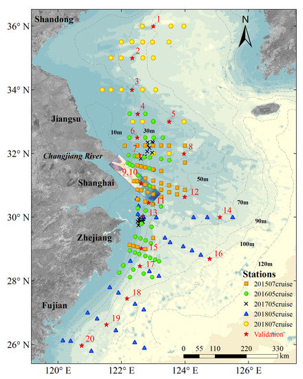
Figure 1.
Sampling locations of 183 stations during the five field campaigns from 2015 to 2018, including 163 stations used for the NNTL construction and 20 numbered stations used for validation, and overlaid with the true color Hyperspectral Imager for the Coastal Ocean (HICO) image used in this study (Section 2.3). The color-coded bathymetry data (GEBCO_2014 Grid, version 20150318) was obtained from GEBCO (http://www.gebco.net/). Depth contours of 10, 30, 50, 70, 90, 100 and 120 m are sketched by gray dashed lines.
2.1.1. Hyperspectral Radiometric Measurements
In situ radiometry measurements including the downwelling spectral irradiance (Ed), sky incoming spectral radiance (Ls), and total radiance of the water (Ltot) were carried out using the Hyperspectral Surface Acquisition System (HyperSAS, Satlantic corporation, Bellevue, WA, USA) by closely following NASA protocols [46]. The Ltot and Ls sensors were pointed to the sea and sky, respectively, at the same nadir and zenith angles between 30° and 50°, with an optimum of 40°. To minimize the sun glint effect, the azimuthal angle of the sensors was set to be within 90°–180° away from the sun, with an optimum of 135° [47,48]. Rrs(λ) was then calculated according to Equation (1):
where λ is the wavelength and ρsky(λ) is the sky radiance spectral reflectance at wavelength λ. The sun glint correction was performed to Rrs according to Busch et al. [49], and the corrected Rrs spectra were interpolated into 1 nm intervals between a wavelength of 370–858 nm.
2.1.2. Taxonomic Species Identification
Samples were fixed with formaldehyde (5%) immediately after collection and transferred back for the laboratory analyses. In the laboratory, phytoplankton cells were first concentrated with 100 mL settlement columns for 24 to 48 h, then identified and counted using an inverted microscope (Olympus corporation, Tokyo, Japan) [50,51]; for the method, we referred mainly to Utermöhl [52]. A total of 242 phytoplankton species were identified, including 129 diatoms, 97 dinoflagellates, 5 chlorophytas, 5 chrysophytas, 4 cyanophytas, 1 xanthophyta, and 1 euglenophyta (the classification was mainly based on http://www.algaebase.org/); after species identification and cell counting, the composition of each species in each station was calculated.
2.1.3. Validation Dataset
For this study, data at 20 stations were selected as the validation dataset (Figure 1), including hyperspectral Rrs data and concurrent data of phytoplankton species composition. In the algorithm validation stage (Section 4.2), by taking the preprocessed spectral data into the NNTL, we then acquired the 26 most abundant phytoplankton species, which together accounted for more than 90% of the cell abundance of all species. A detailed description of the 26 phytoplankton species is listed in Table 1, and the species names are sorted alphabetically.

Table 1.
The 26 most abundant phytoplankton species acquired in the validation dataset used in this study.
2.2. Simulation Dataset
2.2.1. Laboratory Data
Eleven phytoplankton species, namely, three dinoflagellates (Prorocentrum dentatum, zooxanthella, and Karenia mikimotoi), six diatoms (Skeletonema costatum, Thalassiosira weissflogii, Chaetoceros debilis Cleve, Phaeodactylum tricornutum, Chaetoceros curvisetus, and Cyclotella cryptica), one cryptophyta (Heterosigma akashiwo), and one chlorophyte (Nannochloris sp.), which were frequently observed in Chinese ocean regions [7,8,15], were cultured in a laboratory incubator. The temperature was set at 18–20 °C, light intensity was 2500 lx, 12 h light and 12 h dark. The aph(λ) spectra of phytoplankton species were measured using a Lambda-1050 UV/Vis Spectrophotometer (PerkinElmer corporation, Boston, MA, USA). The chlorophyll a concentration (Cph) was measured using a F-2500 Fluorescence Spectrophotometer (Hitachi corporation, Tokyo, Japan). The representative mass-specific absorption spectra (normalized at 440 nm) of the 11 species are shown in Figure 2.
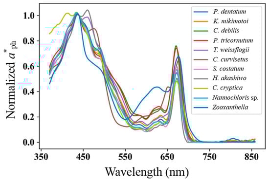
Figure 2.
Representative mass-specific absorption spectra (normalized at 440 nm) of 11 species commonly observed in Chinese ocean regions.
2.2.2. Rrs Simulation Dataset
Semi-analytical models were used to generate Rrs simulation dataset (Equations (2)–(10) in Table 2). The mass-specific absorption spectra of mixed algae a*ph_mix(λ) were calculated using Equation (2), where n1 is the total number of phytoplankton species, a*ph_i(λ) is the ith species’ mass-specific absorption spectra (Section 2.2.1), wi is the composition of ith phytoplankton species, the sum of wi is 1 and can be interpreted as the contribution of each species to the total aph(λ), the range of Cspm was set to 0.1–200 g/m3, the range of Cph was set to 0.1–50 μg/L, and the range of ag(440) was set to 0.01–0.5 m−1. After the variables were set, the Rrs spectra of mixed algae were calculated using Equations (2)–(10). In this study, a total of 200,000 Rrs spectra of mixture algae were generated, and the band range of simulated Rrs was 370–858 nm, with 1 nm intervals, which was consistent with the in situ measurements.
Table 2.
Rrs simulated formulas based on semi-analytical models in this study.
2.3. Satellite Data
One cloud-free HICO image [61] over the Changjiang Estuary was acquired on 28 March 2012 (H2012088004724.L1B_ISS) via the ocean color website (http://oceancolor.gsfc.nasa.gov/) (Figure 1). L1B (Level 1 B: Top of atmosphere radiance) data were processed using SeaDAS software (https://seadas.gsfc.nasa.gov/; version 7.4, NASA, Washington D.C., WA, USA) to first perform a geometric correction, and the atmospheric correction was made using the approach referred to in [62] to generate ocean color Rrs. Then, the Rrs spectra of each pixel was interpolated into 1 nm intervals between 370 and 858 nm. Thereafter, we smoothed the Rrs spectra with a locally weighted scatterplot smoothing (LOWESS) filter [63], and the 2nd derivative spectra of smoothed Rrs spectra were then calculated with a band separation of 27 nm [64] and normalized by the L2-norm (Section 3.2.1).
3. Methods
3.1. Introduction of Transfer Learning
Transfer learning is often used in the scenario, where training and validation data do not feature in the same space or follow the same distribution [65]. Taking a remote sensing application as an example, Jean et al. [66] used high-resolution satellite images and convolutional neural networks to predict poverty in five African countries; with limited training data about socioeconomic indicators, nighttime light intensities were used as a data-rich proxy by the transfer learning method. The results proved that the method is feasible. In the present study, we built a large and general Rrs dataset (200,000 simulated spectra) with 11 common species, and the data volume was adequate to train a reasonable neural network; meanwhile, the phytoplankton species diversity was more abundant in the field measurement Rrs (e.g., there were 242 phytoplankton species during the five cruise investigations from 2015 to 2018). The parameter-transfer approach was used by freezing the first few layers of the trained neural network for the simulation dataset, and updating the last few layers with in situ dataset. This can be accomplished because, for the vast majority of DNNs, the first few layers learn features that are more general and appear not to be specific to a particular dataset or task, and eventually transitions from general to specific in the last few layers [67].
3.2. Transfer Learning for Deep Neural Network Construction
As described in Section 2.2.2, a large general simulation dataset was first generated, and a DNN was subsequently trained using this simulation dataset. However, the trained neural network was not directly applicable for the in situ dataset because of the differences in the numbers, as well as the types of phytoplankton species between the simulation and the in situ datasets. To cope with this challenge, we used the transfer learning technique to transfer part of the knowledge learned from the simulation dataset to the prediction model for the in situ dataset.
3.2.1. Preprocessing for Input Data
Several preprocessing procedures were taken for input data. First, a LOWESS filter (fraction: 0.1; weight function: quadratic function; iterations: 2) was applied to the raw Rrs spectra to minimize random noises [63]. Second, to enhance detailed information about small spectral variations, the 2nd derivative spectra of smoothed Rrs spectra () were calculated according to Equation (11) [68]:
where Δλ = λk−λj = λj−λi, is the band separation, which was set to 27 nm in this study according to Torrecilla et al. [64]. Additionally, to emphasize the shape of the spectra rather than its magnitude, each derivative spectrum was normalized by its L2-norm.
3.2.2. Architecture
A five-layer neural network architecture for the simulation dataset including an input, output, and three hidden layers, i.e., NNsim, was developed. The activation functions of the first two hidden layers were set to be ReLU [69,70], and for the last hidden and output layers, the activation function was set to be Sigmoid and Softmax [71,72], respectively. The dimension of the input layer was 435, the same length as the normalized derivative spectra, and the dimension of the output layer was 11, corresponding to the number of phytoplankton species in the simulation dataset. The dimensions for the hidden layers were 256, 64, and 32, respectively, and the simulation dataset was split into training (90%) and validation (10%) sets. When fitting the model, 90% of the training set was randomly chosen for training and the remaining 10% was used for testing; the Adam optimizer was used [73] and the loss function was set to MAE (mean absolute error); and the training procedure stopped after 800 epochs with a batch size of 512.
The NNTL architecture was defined as the same as that of NNsim, except that the dimension of the output layer was the species number of the in situ dataset, and the batch size was 5. The weights of the first three layers were copied from NNsim and were frozen during the following training procedure, whereas the weights of the last two layers were set to be trainable. Among the 183 in situ samples, 163 were used for training and 20 samples were used for validation (Section 4.2), and at each epoch, NNTL was trained on 130 random choices of samples (80% of the 163 samples) and tested on the remaining 33 samples (20% of the 163 samples). The training procedure stopped after 250 epochs. The flowchart of the method is shown in Figure 3.
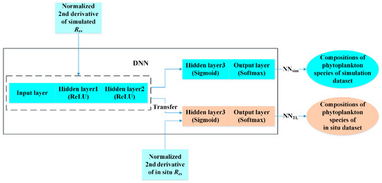
Figure 3.
Workflow of the transfer learning-based deep neural network (DNN) for phytoplankton species composition inversion.
The parameter settings in the model training (data distribution ratios for the simulation dataset and the in situ dataset, the number of dimensions for three hidden layers, the number of the batch size, the number of epochs, the activation functions) in the NNsim and NNTL are the parameter adjustment results. The standards of adjustments are the convergence performance of the loss function in the model training. We conducted tests and found the optimal parameters in this study, as shown in Table 3.
Table 3.
Model parameter adjustment test and optimal options.
The program was coding with keras 2.2.4 (using TensorFlow backend) and Python 3.6.3, and running on a personal computer with CoreTM i7 processor (Intel Corporation, City of Santa Clara, CA, USA) and 20 GB Random Access Memory (RAM). Training the NNsim took about 2 h and 12 min, and training the NNTL took about 3 min. The layers were fully connected. In NNsim, there were 139,723 weights in total and all weights were learnable; in NNTL, there were 147,346 weights in total and 10,066 were learnable and 137,280 were non-learnable. The neural networks were stored as a JavaScript Object Notation (.json) file, and can be called by Python conveniently.
3.3. Accuracy Evaluation
The model performance was evaluated in terms of mean absolute error (MAE), root mean squared error (RMSE), and mean absolute percentage error (MAPE) according to Equations (12)–(14), respectively:
where m is the number of species and n is the number of samples in the training and validation process, is the predicted composition of species j in sample i, and is the true composition of species j in sample i.
4. Results
4.1. Transfer Learning and Neural Network Test
The DNN with transfer learning was tested; in addition, the conventional DNN was considered for comparative analysis. As shown in Figure 4, this includes mainly three parts: NNsim (simulation dataset), NNTL (combined with simulation dataset and in situ dataset), and conventional DNN (combined with simulation dataset and in situ dataset). The convergence process of NNsim is shown in Figure 4a, where MAE decreased rapidly in the first 20 epochs, the rate of descent flattened out with increasing epoch numbers, and we found that, after 800 epochs, MAE was less than 1%, and NNsim tended to be stable. By the transfer learning method, the trained parameters of first few layers in NNsim were preserved, after updating the last few layers with the in situ dataset, NNTL was well constructed (Figure 4b); the convergence process of NNTL was similar to that of NNsim and, after 250 epochs, the MAE of the test set was stable around 4%. The convergence process of the conventional DNN is shown in Figure 4c; the convergence process of the conventional DNN failed due to the enlargement of the MAE with the increasing epoch numbers.
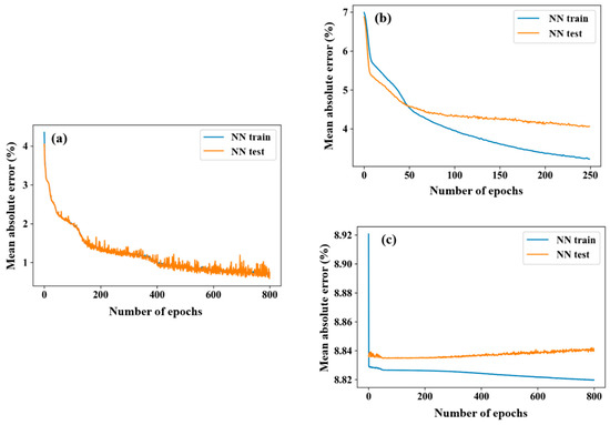
Figure 4.
Mean absolute error (MAE) of training and test sets for (a) NNsim, (b) NNTL and (c) conventional DNN at each epoch.
Further tests of NNsim were conducted. For the randomly selected 10% of the simulation dataset (there are 20,000 spectra), the predicted compositions versus the true compositions are shown in Figure 5. The statistical indicators are as follows: R2 = 0.97, MAE = 0.52%, MAPE = 43.62%, and RMSE = 0.90% on average. The predicted accuracy is acceptable.
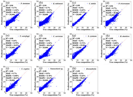
Figure 5.
The NNsim-predicted compositions versus the true compositions of 11 phytoplankton species in the randomly selected 10% of the simulation dataset (there are 20,000 spectra). Namely, (a) P. dentatum, (b) K. mikimotoi, (c) C. debilis, (d) P. tricornutum, (e) T. weissflogii, (f) C. curvisetus, (g) S. costatum, (h) H. akashiwo, (i) C. cryptica, (j) Nannochloris sp., (k) Zooxanthella. The solid line is the 1:1 line.
4.2. Phytoplankton Species Composition Prediction and Validation
Through comparing the in situ and NNTL-predicted compositions (%) in the validation dataset, 26 species were acquired (Section 2.1.3). All species compositions and the sum of the rest of the species compositions (“others”) in each station are presented in the form of stacked bars (Figure 6). Different color columns represent different types of phytoplankton and the height of one column represents the composition of that phytoplankton. At some stations (e.g., stations 7, 8, 9, 13 and 20), specific species (S. costatum, P. delicatissima, P. dentatum, T. thiebaultii) were predominant, whereas at other stations, multiple species co-existed at similar ratios. Generally, NNTL-predicted species compositions were highly consistent with the in situ measurements.
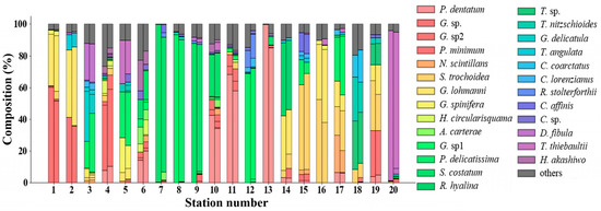
Figure 6.
The phytoplankton species compositions of 20 stations in the validation dataset (Section 2.1). Each station has two stacked bars, with in situ measurements on the left and NNTL-predicted results on the right; the station numbers correspond to validation stations in Figure 1.
Specifically, the statistical indicators of 26 species predicted were calculated (Figure 7): there are 139 points in total (phytoplankton species composition greater than 0), and the in situ measurements and NNTL-predicted results presented a good correlation: R2 = 0.88, MAE = 3.38%, RMSE = 4.4%, and MAPE = 26.08%. In conclusion, the predicted results are acceptable.
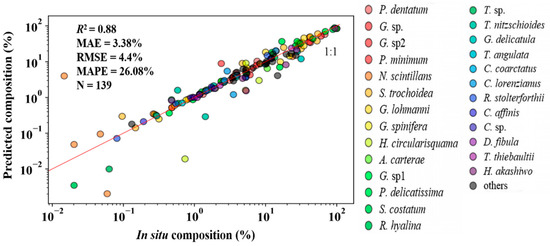
Figure 7.
In situ versus NNTL-predicted compositions (%) of the 26 species in the validation dataset (Section 2.1).
4.3. Phytoplankton Species Composition Prediction from HICO
Through performing HICO data preprocessing (Section 2.3), the normalized 2nd derivative spectra data in each pixel of HICO were obtained, and the dimension of the spectra were kept consistent with the input layer in the NNTL. In the model output phase, we acquired the 12 most abundant species, which together accounted for more than 99% of the cell abundance of all species in each pixel on average. The predicted phytoplankton compositions of these 12 species and the sum of the remaining species (“others”) are shown in Figure 8. The composition of each species varied greatly from each other and, for the same species, the composition varied spatially: among the 12 species, P. dentatum occupied the largest composition from the whole image, whereas S. costatum and P. delicatissima accounted for relatively large proportions near the Changjiang Estuary.
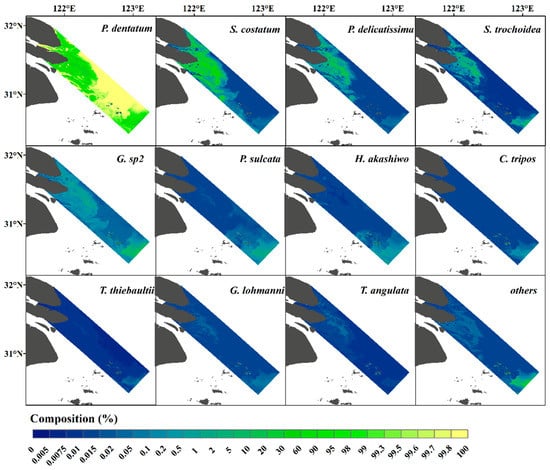
Figure 8.
NNTL-predicted compositions (%) of the 12 most abundant phytoplankton species and sum of the rest of the species (“others”) from HICO imagery, which was acquired on 28 March 2012.
There were no coincident matchups between satellite and in situ observations to validate the predicted species composition. However, Song et al. [74] reported phytoplankton species distributed in this region through a cruise survey carried out from 22 to 28 May 2012, and the sampling range (30.5–32° N, 121.5–123.5° E) basically overlaps with the coverage of HICO. There are five of ten dominant species identified by light microscope in the survey of Song et al. [74], which are consistent with our HICO-predicted results (P. dentatum, Paralia sulcata, P. delicatissima, S. costatum, and S. trochoidea). This investigation validated our predicted results to some extent.
The phytoplankton species compositions are complex and variable, and which are affected by various environmental factors (e.g., temperature, transparency and nutrients) [74]. For example, the ratio of nitrogen to phosphorus (N/P) is considered an important factor influencing community structure; as the N/P increases, the composition of dinoflagellate increases and the composition of diatom decreases [75]. These factors linked to the remote sensing of phytoplankton species composition will be explored in the future.
5. Discussion
5.1. Transfer Learning for Phytoplankton Community
In Section 4.2, the phytoplankton composition inversion at the species level by transfer learning-based DNN was validated, and the predicted results are acceptable (R2 = 0.88, MAE = 3.38%, RMSE = 4.4%, and MAPE = 26.08%). Whether the method is applicable to inversion of phytoplankton composition at the community level is discussed below with respect to related tests and comparative analysis.
5.1.1. DNN Tests for Phytoplankton Community Composition
As mentioned in Section 2.2.1, four communities (11 species) were cultured in the laboratory, and the absorption spectral data were reorganized at the community level. Similar to the research process at the species level, a NNCsim (DNN based on the simulation dataset at the community level) was constructed. Applying the NNCsim to randomly selected 10% of the simulation dataset at the community level, the predicted results are shown in Figure 9, and the statistical indicators are as follows: R2 = 0.99, MAE = 0.43%, RMSE = 0.84%, and MAPE = 17.03% on average.
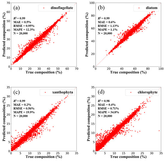
Figure 9.
The NNCsim-predicted compositions versus the true compositions of four phytoplankton communities, namely, (a) dinoflagellate, (b) diatom, (c) xanthophyta, and (d) chlorophyte, in the randomly selected 10% of the simulation dataset at the community level (there are 20,000 spectra). The solid line is the 1:1 line.
Following the DNN tests at the species level, the results are shown in Figure 5, and the statistical indicators are as follows: R2 = 0.97, MAE = 0.52%, MAPE = 43.62%, and RMSE = 0.90% on average. Compared with the predicted accuracy at the species level (MAPE = 43.62%), the accuracy at the community level (MAPE = 17.03%) is improved significantly.
5.1.2. Validation for Phytoplankton Community Composition
A transfer learning-based DNN, combined the simulation dataset with in situ dataset at the community level, short as NNCTL, was also established. The in situ and NNCTL-predicted compositions (%) in the validation dataset (Section 2.1) are shown in Figure 10. The NNCTL-predicted seven community compositions (dinoflagellate, chrysophyta, chlorophyta, xanthophyta, cyanophyta, euglenophyta, and diatom) are highly consistent with the in situ measurements. In addition, the statistical indicators of seven communities predicted were calculated (Figure 11): there are 63 points in total (phytoplankton community composition greater than 0), indicating R2 = 0.99, MAE = 0.33%, MAPE = 1.74%, and RMSE = 1.28%.
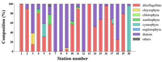
Figure 10.
The phytoplankton community compositions of 20 stations in the validation dataset (Section 2.1). Each station has two stacked bars, with in situ measurements on the left and NNCTL-predicted results on the right; the station numbers correspond to validation stations in Figure 1.
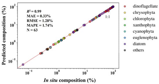
Figure 11.
In situ versus NNCTL-predicted compositions (%) of the seven communities in the validation dataset (Section 2.1).
Through comparing results shown in Figure 6 and Figure 10, the predicted results at the community level are more consistent with the in situ measurement than those at the species level, which is also proved by comparing results shown in Figure 7 and Figure 11. Compared with the predicted accuracy at the species level (MAPE = 26.08%), the predicted accuracy improved by an order of magnitude at the community level (MAPE = 1.74%). Because the types and concentrations of pigments in different species are different, this results in the subtle absorption differences. The pigment difference of different communities is greater than different species. Thus, the DNN may have fewer errors for the prediction at the community level.
5.2. Sensitivity Analysis
Sensitivity analyses of the transfer learning-based DNN were performed under different conditions at the species and community levels. Initially, the optical active components’ effects were considered (Figure 12). It can be seen that, among the three optical active components (Cspm, Cph, ag(440)) considered, the predicted MAPE (%) increased as Cspm increased (Figure 12a), and the variation range was reasonable (maximum of less than 35% at the species level, maximum of less than 17% at the community level) [34], even under relatively high SPM concentrations (180–200 g/m3), which revealed the strong robustness to the SPM of our method. This is very important for phytoplankton species/community composition inversion in optical complex waters, such as in the Changjiang Estuary, where the SPM was dominant in optical active components [76]. Thereafter, MAPE (%) decreased as Cph increased (Figure 12b); because Cph can be regarded as an indicator of phytoplankton biomass [77], our results indicated that the model performance was better in high biomass conditions. However, it was even more remarkable that, under lower Cph conditions, our model still worked well (MAPE less than 35% at the species level, MAPE less than 15% at the community level); therefore, the model feasibility in Case 1 waters is predictable. The CDOM (in terms of ag(440)) had small effects on the model performance (Figure 12c) and the range of variation was less than 4%, possibly because the optical contribution of the CDOM to Rrs was relatively small. All these conclusions prove that our method has reliable prediction results in different water environments.
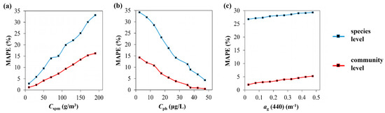
Figure 12.
MAPE (%) of transfer learning-based DNN-predicted results of phytoplankton composition at the species level (blue line) and at the community level (red line) under various conditions of SPM concentration (a), chlorophyll a concentration (b) and CDOM absorption coefficient at 440 nm (c).
The effects of the spectral resolution and signal-to-noise ratio (SNR) to the transfer learning-based DNN at the species and community levels were analyzed synchronously. Different proportions of random noise were added to the simulated and in situ spectral data (at the species and community levels) simultaneously, and the SNR was set as 100, 200, 500, 1000 and +∞ separately. The simulated hyperspectral Rrs and in situ Rrs with 1 nm bandwidth was resampled at different bandwidths synchronously, and the bandwidth was set from 1 to 20 nm and increased at 1 nm intervals. Then, we conducted data preprocessing as described in Section 3.2.1, and the transfer learning-based DNN for specific spectral resolution and SNR at the species and community levels was retrained. Afterward, the transfer learning-based DNN was used to predict phytoplankton species/community compositions under the corresponding spectral resolution and SNR conditions. The results of the accuracy evaluation are shown in Figure 13 (a at the species level and b at the community level). It was found that the MAPE increased with increasing bandwidth and decreased with the increasing SNRs. For the bandwidth greater than 5 nm (species level) and greater than 14 nm (community level), the MAPE increased significantly. The MAPE was 29.61%, 31.46%, 34.56%, and 37.69% (bandwidth equal to 5 nm at the species level), and it was 16.24%, 22.59%, 31.19%, and 34.34% (bandwidth equal to 14 nm at the community level), corresponding to 1000, 500, 200, and 100 of the SNR, respectively. Therefore, for ocean color satellite sensors in the future [78], sensors with bandwidths less than 5 nm at the species level, sensors with bandwidths less than 14 nm at the community level, and concurrently with higher SNR should be recommended.
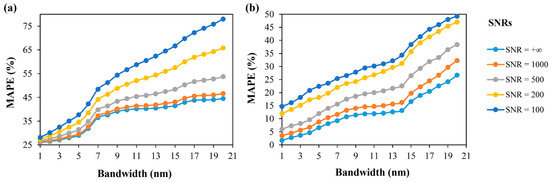
Figure 13.
MAPE (%) of transfer learning-based DNN-predicted composition results at different bandwidths and SNRs: (a) species level, (b) community level.
5.3. Potentials and Limitations
Original domain (simulation dataset) and target domain (in situ dataset) exist in terms of our work, and there are similarities between these domains but they are not identical, which satisfies the precondition for knowledge transfer [65]. We used a mixture of the mass-specific absorption coefficients of 11 phytoplankton species cultures as the input for the simulation dataset, and the predicted results in natural waters were not limited to these 11 species. In addition, the associated composition percentages were also different; in fact, during the learning process for the general simulation dataset, there were about 140,000 nonlinear parameters to solve. Therefore, the general knowledge of phytoplankton species and associated composition was learned well. The optical properties of different species cultivated in the laboratory and natural waters were different, which was related to the associated abundance and growth conditions [79], but they shared similar spectral shapes. This is a disadvantage for traditional methods for distinguishing between them, but is beneficial for general knowledge transfer, as in our study.
Following the transfer learning method, we first used the in situ dataset to update the last layers in the corresponding DNN, which transitions the species information from general to specific as the number of layers increases, and then obtained predictions for phytoplankton species and associated compositions in natural waters. The output of our method is dynamic, and the dominant species and numbers depend on the Rrs spectra and total percentages we set up. For example, in the neural network model for the field measurements (NNTL; Section 4.2), there were 26 species, which together accounted for more than 90% of the cell abundance of all species, and when applied to the HICO imagery (Section 4.3), 12 species were acquired, which totaled 99% of the total cell abundance.
We demonstrated the feasibility of the transfer learning approach in predicting phytoplankton species composition in natural waters. Further improvements could be made to this work. First, as the environment between laboratory measurements and in situ measurements is different [77], more effort should be placed on establishing a more complete simulation dataset, following these steps: 1. More species must be cultivated in the laboratory for optical properties research; 2. The optical properties of mixed species must be taken into consideration; 3. Light, nutrition, and related growth parameters should be connected with optical properties and finally incorporated into the simulation dataset [80]. Second, many factors affect the signal transmission from natural waters to the satellite sensor and much work needs to be done; for example, spectral classification is an effective method for deriving useful information [81], accurate atmospheric correction is also an important research direction [82], and if the atmospheric correction can be done well, combined with other advantages (sensor hardware situations, inversion algorithms, etc.), an accurate inversion of phytoplankton information from space is feasible. In addition, the inversion accuracy still needs to be improved, although transfer learning methods can make up for the deficiency of an in situ dataset to some extent; inversion accuracy could be optimized by increasing the amount of data, especially in situ-measured data. We used semi-analytical models [54,55] for building the simulation Rrs dataset, instead of a more accurate radiative transfer numerical model (e.g., HydroLight) [83]. However, HydroLight requires some time. For instance, we would need more than two months to build the simulation dataset, if 30 s was necessary for 1 spectrum on average, whereas the semi-analytical method only takes a few hours. As the previous study undertaken by Chen [58] has shown, compared with in situ-measured data, semi-analytical models show an underestimation in comparison with HydroLight. Thus, inversion accuracy would possibly decrease more than in a numerical model.
6. Conclusions
In the present study, we presented a machine-learning based phytoplankton species composition inversion method using hyperspectral optical data. First, we trained a deep neural network (NNsim) based on learning from the simulated Rrs dataset; second, we reformed the NNsim into an in situ neural network (NNTL) through the introduction of an in situ Rrs dataset using transfer learning. Using the NNTL, the validation of the predicted results of phytoplankton species composition shows acceptable results in different ocean regions and different cruise campaigns, indicating R2 = 0.88, MAPE = 26.08%, MAE = 3.38%, and RMSE = 4.4%.
Assuming that the types and optical properties of phytoplankton species in one region do not vary considerably, the NNTL can be applied to other hyperspectral measurements, such as the Hyperspectral Imager for the Coastal Ocean (HICO). The HICO-predicted results indicated that the compositions of different phytoplankton species varied considerably between and within species, with uneven spatial distributions. For the Changjiang Estuary, P. dentatum accounted for the largest average composition.
The performances of the transfer learning-based DNN at the species and community levels were analyzed comparatively, and the inversion accuracy at the community level was better than that at the species level (17.03% versus 43.62% in the randomly selected 10% of the simulation dataset, 1.74% versus 26.08% in the validation dataset). Sensitivity analyses indicated that the MAPE increased as SPM concentration increased and chlorophyll a concentration decreased. The signal-to-noise (SNR) and bandwidth also affected the predicted accuracy. The bandwidth smaller than 5 nm at the species level, smaller than 14 nm at the community level, and higher SNR should be suggested for the acceptable accuracy.
As the physics involved in all three methods is different (simulation dataset, in situ measured dataset, and HICO data), we analyzed the effective methods for improving differences between three datasets used in this article, by building a more accurate and complete simulation dataset, accurate atmospheric correction, etc. Moreover, as we only used an in situ dataset collected from five cruises in spring and summer, the types and optical properties of phytoplankton species may change in different seasons. To make the method more applicable, collecting more in situ data should be included in future work. Although the HICO ended operation in 2014, successive hyperspectral satellite missions (e.g., Chinese GF-5 (launched in 2018), scheduled NASA PACE and German EnMAP, etc.) may allow us to have more opportunities of matchups between satellite and in situ data for validation in the future.
Author Contributions
F.S. conceived and organized the research activity. Q.Z. collected field data and laboratory data. Q.Z. and P.S. wrote the programs and performed the experiments, Y.P. performed atmospheric correction of HICO, M.L. checked the language and the figures of the article. All authors contributed to the writing.
Funding
This work was supported by the National Key R&D Program of China (2016YFE0103200), NSFC projects (41771378), and Vulnerabilities and Opportunities of the Coastal Ocean (VOCO, No. SKLEC-2016RCDW01). The research is a part of the HYPERMAQ project (SR/00/335) of the BELSPO Research programme for Earth Observation STEREO III, commissioned and financed by the Belgian Science Policy Office.
Acknowledgments
We would like to thank NASA GSFC for providing HICO data (https://oceancolor.gsfc.nasa.gov/). In situ data in the Yellow Sea and East China Sea from 2015 to 2018 were obtained from the “Runjiang 1”, “Zhehaike 1”, “Zheyuke 2”, “Dongfanghong 2”, and “Xiangyanghong 18” cruise campaigns, and the participation of all the scientists and crew in the field surveys is sincerely appreciated. We are grateful to the team of Yue Gao from Xiamen University for helping with the laboratory analysis of phytoplankton species in the cruise surveyed in May 2016 and Richard G. J. Bellerby from East China Normal University for the collection and laboratory analysis of phytoplankton species in the cruise surveyed in May 2017 in this work. The authors also greatly appreciate anonymous reviewers for their constructive comments and suggestions.
Conflicts of Interest
The authors declare no conflict of interest.
References
- Smetacek, V.; Cloern, J.E. Oceans-On phytoplankton trends. Science 2008, 319, 1346–1348. [Google Scholar] [CrossRef] [PubMed]
- Boyce, D.G.; Lewis, M.R.; Worm, B. Global phytoplankton decline over the past century. Nature 2010, 466, 591–595. [Google Scholar] [CrossRef] [PubMed]
- Armbrust, E.V. The life of diatoms in the world’s oceans. Nature 2009, 459, 185–192. [Google Scholar] [CrossRef] [PubMed]
- Platt, T.; Fuentes-Yaco, C.; Frank, K.T. Spring algal bloom and larval fish survival. Nature 2003, 423, 398–399. [Google Scholar] [CrossRef] [PubMed]
- Schubert, C.J.; Villanueva, J.; Calvert, S.E.; Cowie, G.L.; von Rad, U.; Schulz, H.; Berner, U.; Erlenkeuser, H. Stable phytoplankton community structure in the Arabian Sea over the past 200,000 years. Nature 1998, 394, 563–566. [Google Scholar] [CrossRef]
- Aiken, J. Phytoplankton functional types from space. In Reports of the International Ocean-Colour Coordinating Group, No. 15; Sathyendranath, S., Ed.; IOCCG: Dartmouth, NS, Canada, 2014; pp. 9–15. [Google Scholar]
- Li, Z. Phytoplankton Community and Its Related Carbon Sinking in the Changjiang (Yangtze River) Estuary and Adjacent Waters. Ph.D. Thesis, Institute of Oceanology, Chinese Academy of Sciences, Qingdao, China, June 2018. [Google Scholar]
- Boopathi, T.; Lee, J.; Youn, S.H.; Ki, J. Temporal and spatial dynamics of phytoplankton diversity in the East China Sea near Jeju Island (Korea): A pyrosequencing-based study. Biochem. Syst. Ecol. 2015, 63, 143–152. [Google Scholar] [CrossRef]
- Zhu, Q.; Li, J.; Zhang, F.; Shen, Q. Distinguishing Cyanobacterial Bloom from Floating Leaf Vegetation in Lake Taihu Based on Medium-Resolution Imaging Spectrometer (MERIS) Data. IEEE J. Sel. Top. Appl. Earth Obs. Remote Sens. 2018, 11, 34–44. [Google Scholar] [CrossRef]
- Bracher, A.; Bouman, H.A.; Brewin, R.J.W.; Bricaud, A.; Brotas, V.; Ciotti, A.M.; Clementson, L.; Devred, E.; Di Cicco, A.; Dutkiewicz, S.; et al. Obtaining Phytoplankton Diversity from Ocean Color: A Scientific Roadmap for Future Development. Front. Mar. Sci. 2017, 4, 55. [Google Scholar] [CrossRef]
- Mouw, C.B.; Hardman-Mountford, N.J.; Alvain, S.; Bracher, A.; Brewin, R.J.W.; Bricaud, A.; Ciotti, A.M.; Devred, E.; Fujiwara, A.; Hirata, T.; et al. A Consumer’s Guide to Satellite Remote Sensing of Multiple Phytoplankton Groups in the Global Ocean. Front. Mar. Sci. 2017, 4, 41. [Google Scholar] [CrossRef]
- Whitmire, A.L.; Pegau, W.S.; Karp-Boss, L.; Boss, E.; Cowles, T.J. Spectral backscattering properties of marine phytoplankton cultures. Opt. Express 2010, 18, 15073–15093. [Google Scholar] [CrossRef]
- Zhou, W.; Wang, G.; Sun, Z.; Cao, W.; Xu, Z.; Hu, S.; Zhao, J. Variations in the optical scattering properties of phytoplankton cultures. Opt. Express 2012, 20, 11189–11206. [Google Scholar] [CrossRef] [PubMed]
- Kurekin, A.A.; Miller, P.I.; Van der Woerd, H.J. Satellite discrimination of Karenia mikimotoi and Phaeocystis harmful algal blooms in European coastal waters: Merged classification of ocean colour data. Harmful Algae 2014, 31, 163–176. [Google Scholar] [CrossRef] [PubMed]
- Tao, B.; Mao, Z.; Lei, H.; Pan, D.; Shen, Y.; Bai, Y.; Zhu, Q.; Li, Z. A novel method for discriminating Prorocentrum donghaiense from diatom blooms in the East China Sea using MODIS measurements. Remote Sens. Environ. 2015, 158, 267–280. [Google Scholar] [CrossRef]
- Tao, B.; Mao, Z.; Lei, H.; Pan, D.; Bai, Y.; Zhu, Q.; Zhang, Z. A semianalytical MERIS green-red band algorithm for identifying phytoplankton bloom types in the East China Sea. J. Geophys. Res. Ocean. 2016, 122, 1772–1788. [Google Scholar] [CrossRef]
- Shang, S.; Wu, J.; Huang, B.; Lin, G.; Lee, Z.; Liu, J.; Shang, S. A new approach to discriminate dinoflagellate from diatom blooms from space in the East China Sea. J. Geophys. Res. Ocean. 2014, 119, 4653–4668. [Google Scholar] [CrossRef]
- Alvain, S.; Moulin, C.; Dandonneau, Y.; Bréon, F.M. Remote sensing of phytoplankton groups in case 1 waters from global SeaWiFS imagery. Deep Sea Res. II 2005, 52, 1989–2004. [Google Scholar] [CrossRef]
- Alvain, S.; Loisel, H.; Dessailly, D. Theoretical analysis of ocean color radiances anomalies and implications for phytoplankton groups detection in case 1 waters. Opt. Express 2012, 20, 1070–1083. [Google Scholar] [CrossRef]
- Isada, T.; Hirawake, T.; Kobayashi, T.; Nosaka, Y.; Natsuike, M.; Imai, I.; Suzuki, K.; Saitoh, S.I. Hyperspectral optical discrimination of phytoplankton community structure in Funka Bay and its implications for ocean color remote sensing of diatoms. Remote Sens. Environ. 2015, 159, 134–151. [Google Scholar] [CrossRef]
- Kostadinov, T.S.; Cabré, A.; Vedantham, H.; Marinov, I.; Bracher, A.; Brewin, R.J.W.; Bricaud, A.; Hirata, T.; Hirawake, T.; Hardman-Mountford, N.J.; et al. Inter-comparison of phytoplankton functional type phenology metrics derived from ocean color algorithms and Earth System Models. Remote Sens. Environ. 2017, 190, 162–177. [Google Scholar] [CrossRef]
- Kramer, S.J.; Roesler, C.S.; Sosik, H.M. Bio-optical discrimination of diatoms from other phytoplankton in the surface ocean: Evaluation and refinement of a model for the Northwest Atlantic. Remote Sens. Environ. 2018, 217, 126–143. [Google Scholar] [CrossRef]
- Sathyendranath, S.; Watts, L.; Devred, E.; Platt, T.; Caverhill, C.; Maass, H. Discrimination of diatoms from other phytoplankton using ocean-colour data. Mar. Ecol. Prog. Ser. 2004, 272, 59–68. [Google Scholar] [CrossRef]
- Uitz, J.; Stramski, D.; Reynolds, R.A.; Dubranna, J. Assessing phytoplankton community composition from hyperspectral measurements of phytoplankton absorption coefficient and remote-sensing reflectance in open-ocean environments. Remote Sens. Environ. 2015, 171, 58–74. [Google Scholar] [CrossRef]
- Craig, S.E.; Lohrenz, S.E.; Lee, Z.; Mahoney, K.L.; Kirkpatrick, G.J.; Schofield, O.M.; Steward, R.G. Use of hyperspectral remote sensing reflectance for detection and assessment of the harmful alga, Karenia brevis. Appl. Opt. 2006, 45, 5414–5425. [Google Scholar] [CrossRef]
- Mao, Z.; Stuart, V.; Pan, D.; Chen, J.; Gong, F.; Huang, H.; Zhu, Q. Effects of phytoplankton species composition on absorption spectra and modeled hyperspectral reflectance. Ecol. Inform. 2010, 5, 359–366. [Google Scholar] [CrossRef]
- Millie, D.F.; Schofield, O.M.; Kirkpatrick, G.J.; Johnsen, G.; Tester, P.A.; Vinyard, B.T. Detection of harmful algal blooms using photopigments and absorption signatures: A case study of the Florida red tide dinoflagellate, Gymnodinium breve. Limnol. Oceanogr. 1997, 42, 1240–1251. [Google Scholar] [CrossRef]
- Xi, H.; Hieronymi, M.; Röttgers, R.; Krasemann, H.; Qiu, Z. Hyperspectral Differentiation of Phytoplankton Taxonomic Groups: A Comparison between Using Remote Sensing Reflectance and Absorption Spectra. Remote Sens. 2015, 7, 14781–14805. [Google Scholar] [CrossRef]
- Xi, H.; Hieronymi, M.; Krasemann, H.; Röttgers, R. Phytoplankton Group Identification Using Simulated and in situ Hyperspectral Remote Sensing Reflectance. Front. Mar. Sci. 2017, 4, 1–13. [Google Scholar] [CrossRef]
- Mackey, M.; Mackey, D.; Higgins, H.; Wright, S. CHEMTAX-a program for estimating class abundances from chemical markers: Application to HPLC measurements of phytoplankton. Mar. Ecol. Prog. Ser. 1996, 144, 265–283. [Google Scholar] [CrossRef]
- Pan, X.; Mannino, A.; Russ, M.E.; Hooker, S.B.; Harding, L.W., Jr. Remote sensing of phytoplankton pigment distribution in the United States northeast coast. Remote Sens. Environ. 2010, 114, 2403–2416. [Google Scholar] [CrossRef]
- Pan, X.; Mannino, A.; Marshall, H.G.; Filippino, K.C.; Mulholland, M.R. Remote sensing of phytoplankton community composition along the northeast coast of the United States. Remote Sens. Environ. 2011, 115, 3731–3747. [Google Scholar] [CrossRef]
- Pan, X.; Wong, G.T.F.; Ho, T.; Shiah, F.; Liu, H. Remote sensing of picophytoplankton distribution in the northern South China Sea. Remote Sens. Environ. 2013, 128, 162–175. [Google Scholar] [CrossRef]
- Zhang, H.; Devred, E.; Fujiwara, A.; Qiu, Z.; Liu, X. Estimation of phytoplankton taxonomic groups in the Arctic Ocean using phytoplankton absorption properties: Implication for ocean-color remote sensing. Opt. Express 2018, 26, 32280. [Google Scholar] [CrossRef]
- Harrison, J.W.; Howell, E.T.; Watson, S.B.; Smith, R.E.H. Improved estimates of phytoplankton community composition based on in situ spectral fluorescence: Use of ordination and field-derived norm spectra for the bbe FluoroProbe. Can. J. Fish. Aquat. Sci. 2016, 73, 1472–1482. [Google Scholar] [CrossRef]
- Wang, S.; Xiao, C.; Ishizaka, J.; Qiu, Z.; Sun, D.; Xu, Q.; Zhu, Y.; Huan, Y.; Watanabe, Y. Statistical approach for the retrieval of phytoplankton community structures from in situ fluorescence measurements. Opt. Express 2016, 24, 23635. [Google Scholar] [CrossRef]
- Ling, Z.; Sun, D.; Wang, S.; Qiu, Z.; Huan, Y.; Mao, Z.; He, Y. Retrievals of phytoplankton community structures from in situ fluorescence measurements by HS-6P. Opt. Express 2018, 26, 30556. [Google Scholar] [CrossRef]
- Raitsos, D.E.; Lavender, S.J.; Maravelias, C.D.; Haralabous, J.; Richardson, A.J.; Reid, P.C. Identifying four phytoplankton functional types from space: An ecological approach. Limnol. Oceanogr. 2008, 53, 605–613. [Google Scholar] [CrossRef]
- Palacz, A.P.; John, M.A.S.; Brewin, R.J.W.; Hirata, T.; Gregg, W.W. Distribution of phytoplankton functional types in high-nitrate, low-chlorophyll waters in a new diagnostic ecological indicator mode. Biogeosciences 2013, 10, 8103–8157. [Google Scholar] [CrossRef]
- Reichstein, M.; Camps-Valls, G.; Stevens, B.; Jung, M.; Denzler, J.; Carvalhais, N.; Prabhat. Deep learning and process understanding for data-driven Earth system science. Nature 2019, 566, 195–204. [Google Scholar] [CrossRef]
- Chang, N.; Xuan, Z.; Yang, Y.J. Exploring spatiotemporal patterns of phosphorus concentrations in a coastal bay with MODIS images and machine learning models. Remote Sens. Environ. 2013, 134, 100–110. [Google Scholar] [CrossRef]
- Qiu, Z.; Li, Z.; Bilal, M.; Wang, S.; Sun, D.; Chen, Y. Automatic method to monitor floating macroalgae blooms based on multilayer perceptron: Case study of Yellow Sea using GOCI images. Opt. Express 2018, 26, 26810. [Google Scholar] [CrossRef]
- Song, W.; Dolan, J.M.; Cline, D.; Xiong, G. Learning-Based Algal Bloom Event Recognition for Oceanographic Decision Support System Using Remote Sensing Data. Remote Sens. 2015, 7, 13564–13585. [Google Scholar] [CrossRef]
- Wu, X.; Kumar, V.; Quinlan, J.R.; Ghosh, J.; Yang, Q.; Motoda, H.; McLachlan, G.J.; Ng, A.; Liu, B.; Yu, P.S.; et al. Top 10 algorithms in data mining. Knowl. Inf. Syst. 2008, 14, 1–37. [Google Scholar] [CrossRef]
- Ling, X.; Dai, W.; Xue, G.; Yang, Q.; Yu, Y. Spectral Domain-Transfer Learning. In Proceedings of the 14th ACM SIGKDD International Conference on Knowledge Discovery and Data Mining, Las Vegas, NV, USA, 24–27 August 2008. [Google Scholar]
- Mueller, J.L.; Fargion, G.S.; McClain, C.R.; Mueller, J.; Brown, S.; Clark, D.; Johnson, B.; Yoon, H.; Lykke, K.; Flora, S. Ocean Optics Protocols for Satellite Ocean Color Sensor Validation Volume VI: Special Topics in Ocean Optics Protocols, Part 2; NASA: Washington, DC, USA, 2004; Volume 211621.
- Shang, P.; Shen, F. Atmospheric Correction of Satellite GF-1/WFV Imagery and Quantitative Estimation of Suspended Particulate Matter in the Yangtze Estuary. Sensors 2016, 16, 1997. [Google Scholar] [CrossRef]
- Sokoletsky, L.G.; Shen, F. Optical closure for remote-sensing reflectance based on accurate radiative transfer approximations: The case of the Changjiang (Yangtze) River Estuary and its adjacent coastal area, China. Int. J. Remote Sens. 2014, 35, 4193–4224. [Google Scholar] [CrossRef]
- Busch, J.A.; Hedley, J.D.; Zielinski, O. Correction of hyperspectral reflectance measurements for surface objects and direct sun reflection on surface waters. Int. J. Remote Sens. 2013, 34, 6651–6667. [Google Scholar] [CrossRef]
- Guo, S.; Feng, Y.; Wang, L.; Dai, M.; Liu, Z.; Bai, Y.; Sun, J. Seasonal variation in the phytoplankton community of a continental-shelf sea: The East China Sea. Mar. Ecol. Prog. Ser. 2014, 516, 103–126. [Google Scholar] [CrossRef]
- Guo, S.; Sun, J.; Zhao, Q.; Feng, Y.; Huang, D.; Liu, S. Sinking rates of phytoplankton in the Changjiang (Yangtze River) estuary: A comparative study between Prorocentrum dentatum and Skeletonema dorhnii bloom. J. Mar. Syst. 2016, 154, 5–14. [Google Scholar] [CrossRef]
- Utermöhl, H. Zur vervollkommung der quantitativen phytoplankton-methodik. Limnology 1958, 9, 263–272. [Google Scholar]
- Bricaud, A.; Babin, M.; Morel, A.; Claustre, H. Variability in the chlorophyll-specific absorption coefficients of natural phytoplankton: Analysis and parameterization. J. Geophys. Res. Ocean. 1995, 100, 13321–13332. [Google Scholar] [CrossRef]
- Lee, Z.; Carder, K.L.; Arnone, R.A. Deriving inherent optical properties from water color: A multiband quasi-analytical algorithm for optically deep waters. Appl. Opt. 2002, 41, 5755–5772. [Google Scholar] [CrossRef]
- Gordon, H.R.; Brown, O.B.; Evans, R.H.; Brown, J.W.; Smith, R.C.; Baker, K.S.; Clark, D.K. A semianalytic radiance model of ocean color. J. Geophys. Res. Ocean. 1988, 93, 10909–10924. [Google Scholar] [CrossRef]
- Mobley, C.D. Light and Water-Radiative Transfer in Natural Waters; Academic Press: San Diego, CA, USA, 1994; pp. 86–100. [Google Scholar]
- Liu, M. Scattering Properties of Suspended Particles in High Turbid Waters and Remote Sensing Application. Master’s Thesis, State Key Laboratory of Estuarine and Coastal Science, East China Normal University, Shanghai, China, June 2013. [Google Scholar]
- Chen, Y. Calculation of Remote Sensing Reflectance Based on Radiative Transfer Model and Analysis of Chlorophyll Retrieval Algorithm. Master’s Thesis, State Key Laboratory of Estuarine and Coastal Science, East China Normal University, Shanghai, China, June 2015. [Google Scholar]
- Yu, X. Measurements of Pigment Absorption Coefficients and Retrieval Models of Pigment Concentration in Turbid Coastal Waters. Master’s Thesis, State Key Laboratory of Estuarine and Coastal Science, East China Normal University, Shanghai, China, June 2013. [Google Scholar]
- Shen, F.; Zhou, Y.; Hong, G. Absorption Property of Non-algal Particles and Contribution to Total Light Absorption in Optically Complex Waters, a Case Study in Yangtze Estuary and Adjacent Coast. In Proceedings of the International Conference on Remote Sensing, Hangzhou, Zhejiang, China, 5–6 October 2010. [Google Scholar]
- Lucke, R.L.; Corson, M.; McGlothlin, N.R.; Butcher, S.D.; Wood, D.L.; Korwan, D.R.; Li, R.R.; Snyder, W.A.; Davis, C.O.; Chen, D.T. Hyperspectral Imager for the Coastal Ocean: Instrument description and first images. Appl. Opt. 2015, 50, 1501–1516. [Google Scholar] [CrossRef]
- Pan, Y. Studies on Atmospheric Correction Methods and Remote Sensing Inversions of Typical Ocean Color Parameters over Turbid Waters. Ph.D. Thesis, State Key Laboratory of Estuarine and Coastal Science, East China Normal University, Shanghai, China, June 2018. [Google Scholar]
- Cleveland, W.S. LOWESS: A Program for Smoothing Scatterplots by Robust Locally Weighted Regression. Am. Stat. 1981, 35, 54. [Google Scholar] [CrossRef]
- Torrecilla, E.; Stramski, D.; Reynolds, R.A.; Millán-Núñez, E.; Piera, J. Cluster analysis of hyperspectral optical data for discriminating phytoplankton pigment assemblages in the open ocean. Remote Sens. Environ. 2011, 115, 2578–2593. [Google Scholar] [CrossRef]
- Pan, S.J.; Yang, Q. A Survey on Transfer Learning. IEEE Trans. Knowl. Data Eng. 2010, 22, 1345–1369. [Google Scholar] [CrossRef]
- Jean, N.; Burke, M.; Xie, M.; Davis, W.M.; Lobell, D.B.; Ermon, S. Combining satellite imagery and machine learning to predict poverty. Science 2016, 353, 790–794. [Google Scholar] [CrossRef]
- Yosinski, J.; Clune, J.; Bengio, Y.; Lipson, H. How transferable are features in deep neural networks? In Proceedings of the 27th International Conference on Neural Information Processing Systems, Montreal, QC, Canada, 8–13 December 2014.
- Tsai, F.; Philpot, W. Derivative Analysis of Hyperspectral Data. Remote Sens. Environ. 1998, 66, 41–51. [Google Scholar] [CrossRef]
- Hahnloser, R.H.R.; Sarpeshkar, R.; Mahowald, M.A.; Douglas, R.J.; Seung, H.S. Digital selection and analogue amplication coexist in a cortex-inspired silicon circuit. Nature 2000, 405, 947–951. [Google Scholar] [CrossRef]
- Hahnloser, R.H.R.; Seung, H.S.; Slotine, J.J. Permitted and forbidden sets in symmetric threshold-linear networks. Neural Comput. 2003, 15, 621–638. [Google Scholar] [CrossRef]
- Bishop, C.M. Pattern Recognition and Machine Learning (Information Science and Statistics); Springer: New York, NY, USA, 2006. [Google Scholar]
- Han, J.; Moraga, C. The influence of the sigmoid function parameters on the speed of backpropagation learning. In Proceedings of the International Workshop on Artificial Neural Networks: From Natural to Artificial Neural Computation, Torremolinos, Malaga, Spain, 7–9 June 1995. [Google Scholar]
- Kingma, D.; Ba, J. Adam: A Method for Stochastic Optimization. In Proceedings of the 3rd the International Conference on Learning Representations, San Diego, CA, USA, 7–9 May 2015. [Google Scholar]
- Song, S.; Li, Z.; Li, C.; Yu, Z. The response of spring phytoplankton assemblage to diluted water and upwelling in the eutrophic Changjiang (Yangtze River) Estuary. Acta Oceanol. Sin. 2017, 36, 101–110. [Google Scholar] [CrossRef]
- Li, Z.; Song, S.; Li, C.; Yu, Z. Preliminary discussion on the phytoplankton assemblages and its response to the environmental changes in the Changjiang (Yangtze) River Estuary and its adjacent waters during the dry season and the wet season. Acta Oceanol. Sin. 2017, 39, 122–144. [Google Scholar]
- Shen, F.; Verhoef, W.; Zhou, Y.; Salama, M.S.; Liu, X. Satellite Estimates of Wide-Range Suspended Sediment Concentrations in Changjiang (Yangtze) Estuary Using MERIS Data. Estuaries Coasts 2010, 33, 1420–1429. [Google Scholar] [CrossRef]
- Arnone, R. Remote sensing of ocean colour in coastal, and other optically-complex, waters. In Reports of the International Ocean-Colour Coordinating Group, No. 3; Sathyendranath, S., Ed.; IOCCG: Dartmouth, NS, Canada, 2000; pp. 11–22. [Google Scholar]
- Ahn, Y.H. Mission requirements for future ocean-colour sensors. In Reports of the International Ocean-Colour Coordinating Group, No. 12; McClain, C.R., Meister, G., Eds.; IOCCG: Dartmouth, NS, Canada, 2012; pp. 42–45. [Google Scholar]
- Nair, A.; Sathyendranath, S.; Platt, T.; Morales, J.; Stuart, V.; Forget, M.; Devred, E.; Bouman, H. Remote sensing of phytoplankton functional types. Remote Sens. Environ. 2008, 112, 3366–3375. [Google Scholar] [CrossRef]
- Organelli, E.; Nuccio, C.; Lazzara, L.; Uitz, J.; Bricaud, A.; Massi, L. On the discrimination of multiple phytoplankton groups from light absorption spectra of assemblages with mixed taxonomic composition and variable light conditions. Appl. Opt. 2017, 56, 3952–3968. [Google Scholar] [CrossRef]
- Dilip, K.P.; Krishna, A. Classification of Hyperspectral or Trichromatic Measurements of Ocean Color Data into Spectral Classes. Sensors 2016, 16, 413–432. [Google Scholar]
- Pan, Y.; Shen, F.; Verhoef, W. An improved spectral optimization algorithm for atmospheric correction over turbid coastal waters: A case study from the Changjiang (Yangtze) estuary and the adjacent coast. Remote Sens. Environ. 2017, 191, 197–214. [Google Scholar] [CrossRef]
- Mobley, C.D. Hydrolight 3. 0 User’s Guide (Final Report); International Stanford Research Institute: Menlo Park, CA, USA, 1995. [Google Scholar]
© 2019 by the authors. Licensee MDPI, Basel, Switzerland. This article is an open access article distributed under the terms and conditions of the Creative Commons Attribution (CC BY) license (http://creativecommons.org/licenses/by/4.0/).