Forest Damage Assessment Using Deep Learning on High Resolution Remote Sensing Data


Abstract
1. Introduction
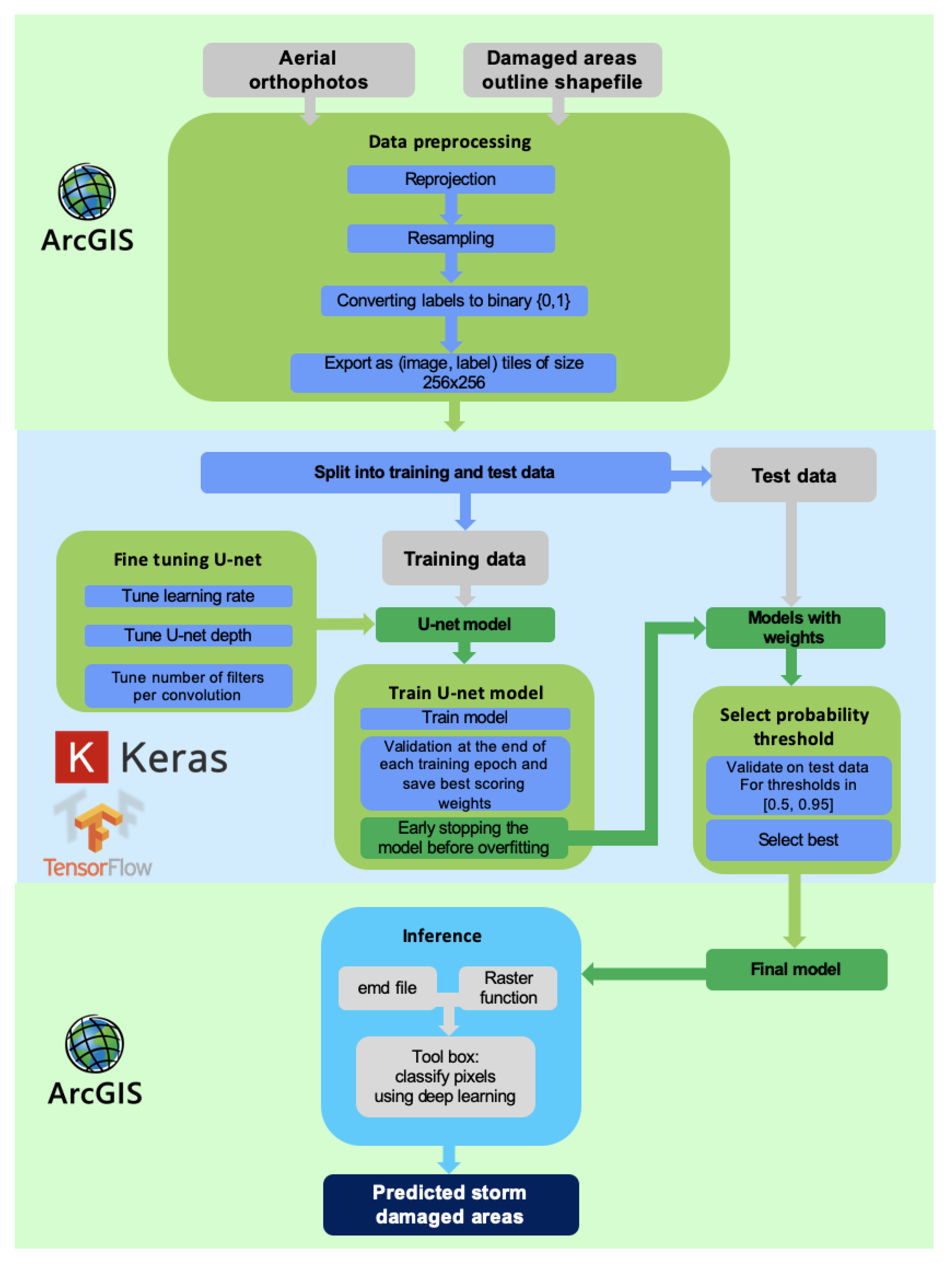
2. Materials and Methods
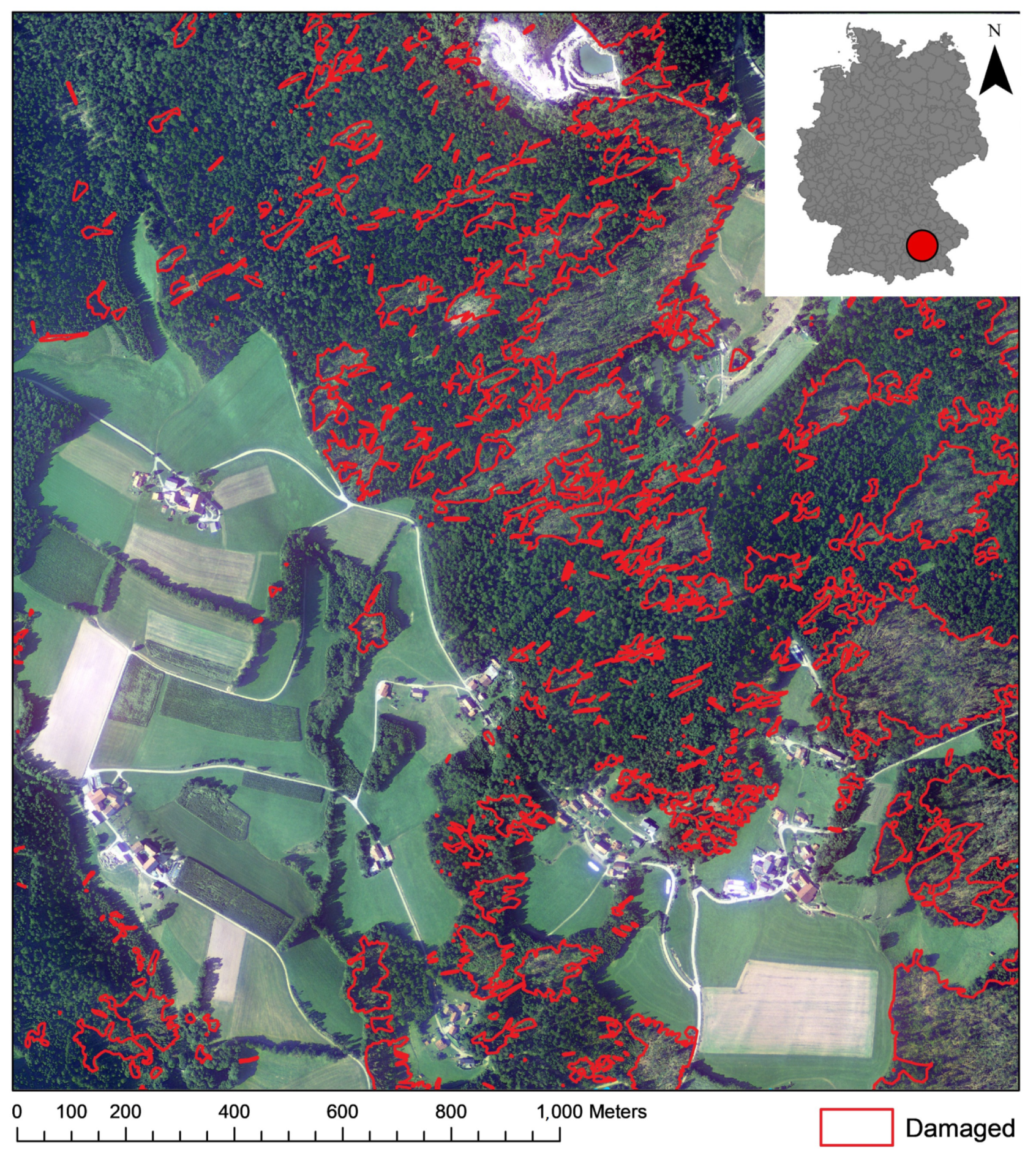
2.1. Data
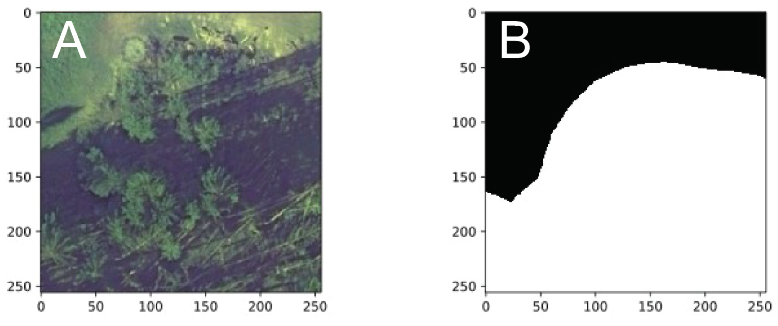
2.2. Data Preprocessing
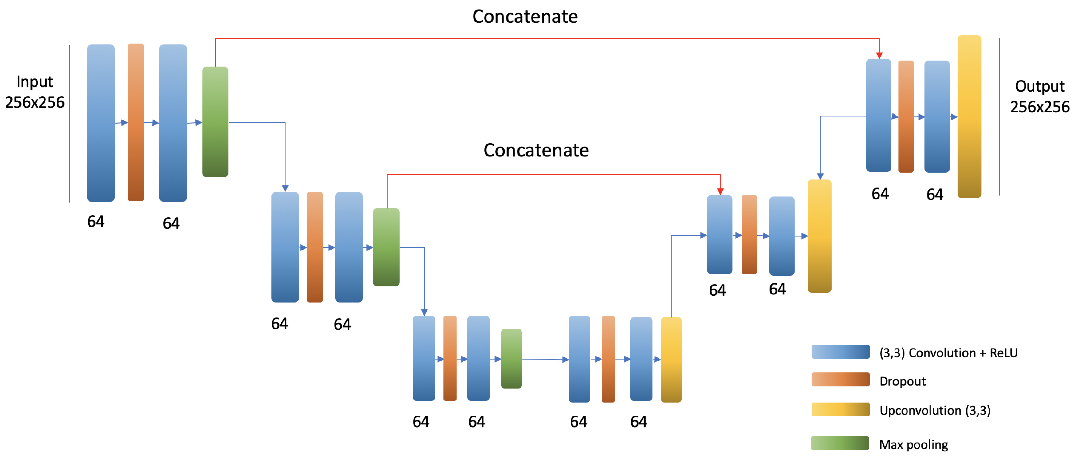
2.3. CNN Architecture
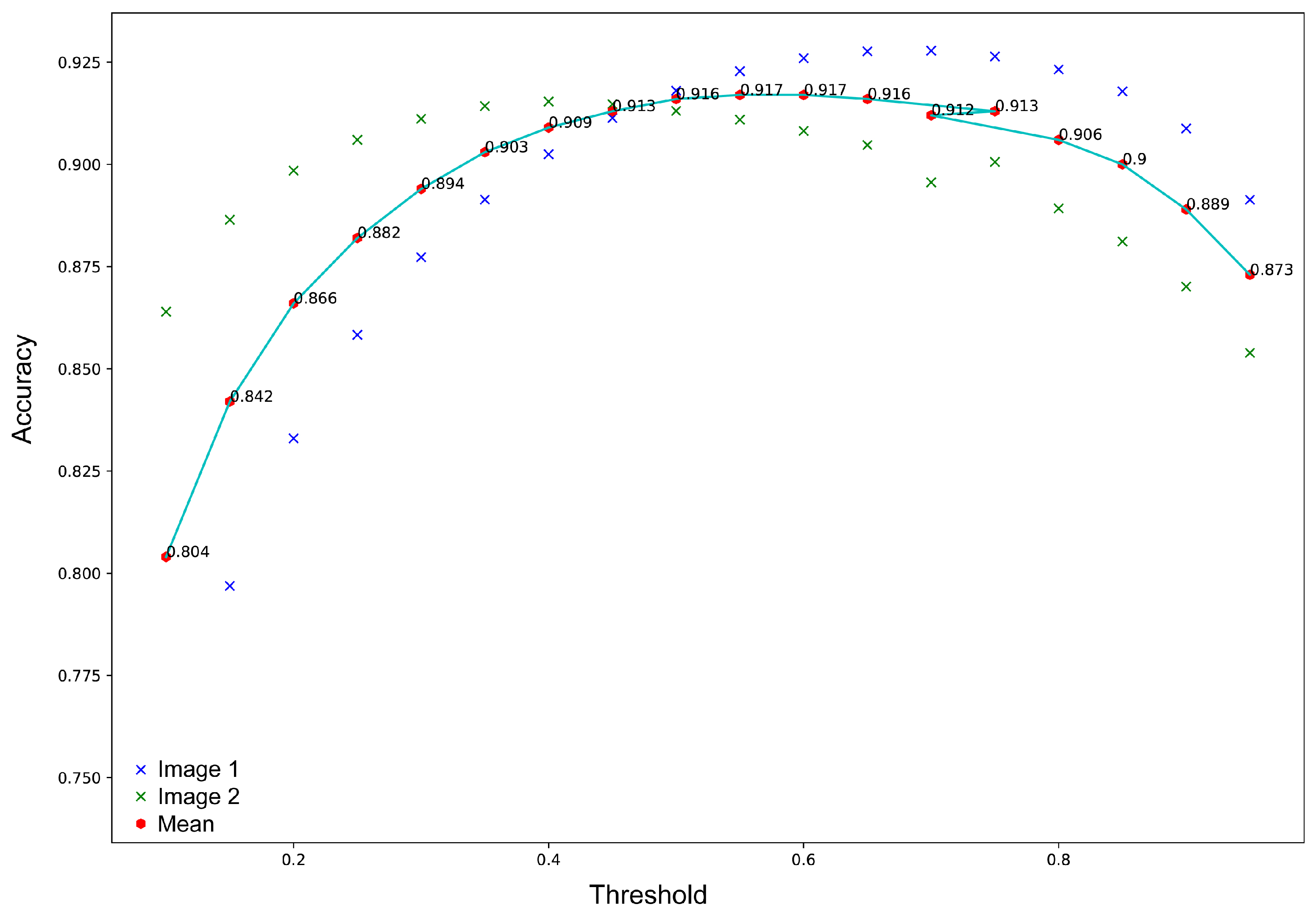
2.4. Evaluation Metrics
| Algorithm 1 Pseudocode for calculating a custom metric for thresholding. |
| 1: Create an empty array to hold the intersection over union values for all thresholds IoUs |
| 2: |
| 3: Create array V of values between 0.5 and 1 with a step of 0.05 |
| 4: |
| 5: Feed forward to do the pixelwise classification prediction |
| 6: |
| 7: for Every element k of array V do |
| 8: |
| 9: Compute confusion matrix elements for the threshold set at k |
| 10: |
| 11: Compute the intersection over union for threshold k |
| 12: |
| 13: Append the computed intersection over union for threshold k in array |
| 14: |
| 15: end for |
| 16: |
| 17: return the mean intersection over union |
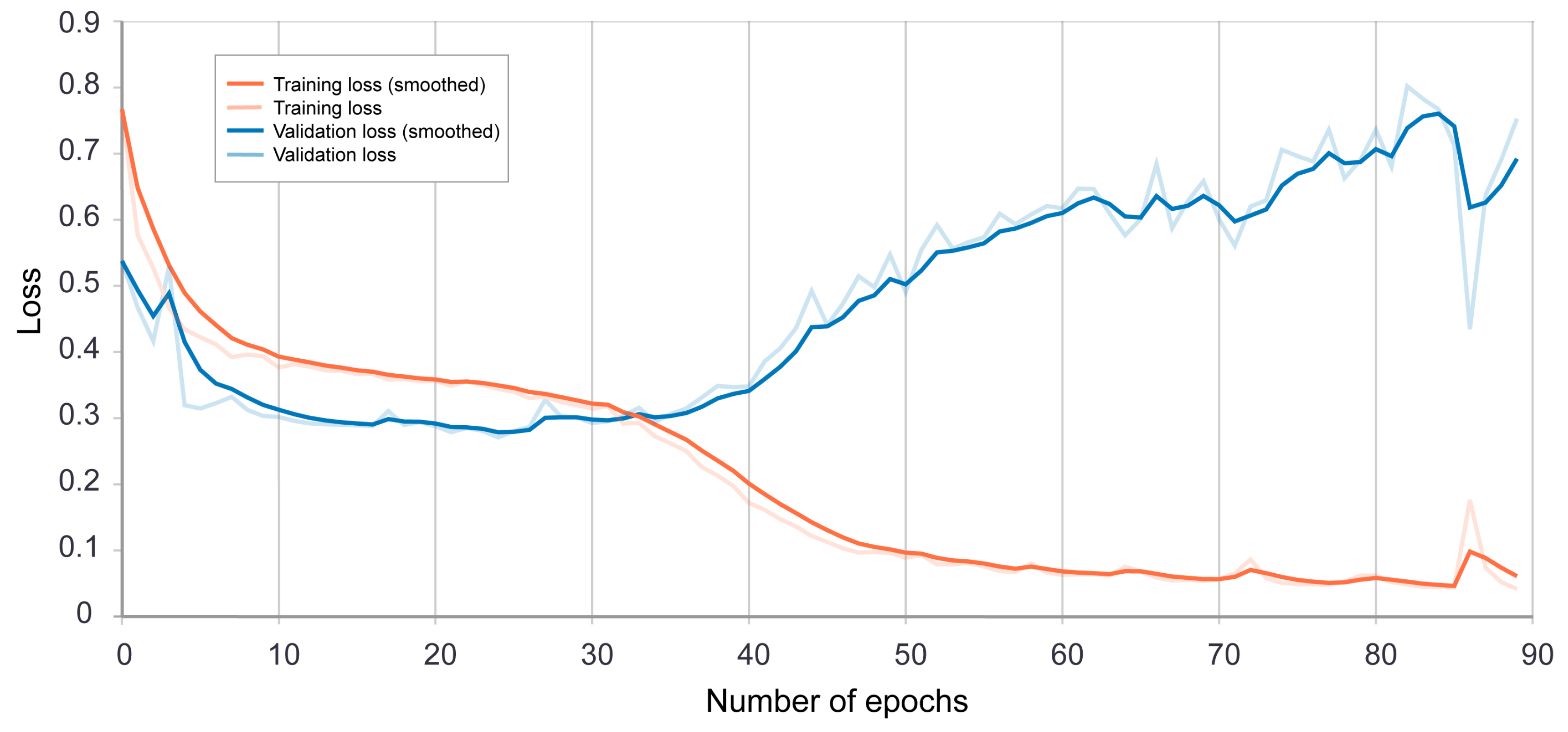
2.5. Training and Fine-Tuning of the U-Net Model
2.5.1. Encoding Path
2.5.2. Decoding Path
2.6. Comparison to a Support Vector Machine Classifier and a Random Forest Algorithm
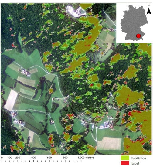
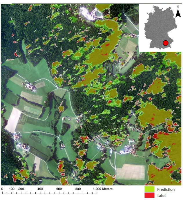
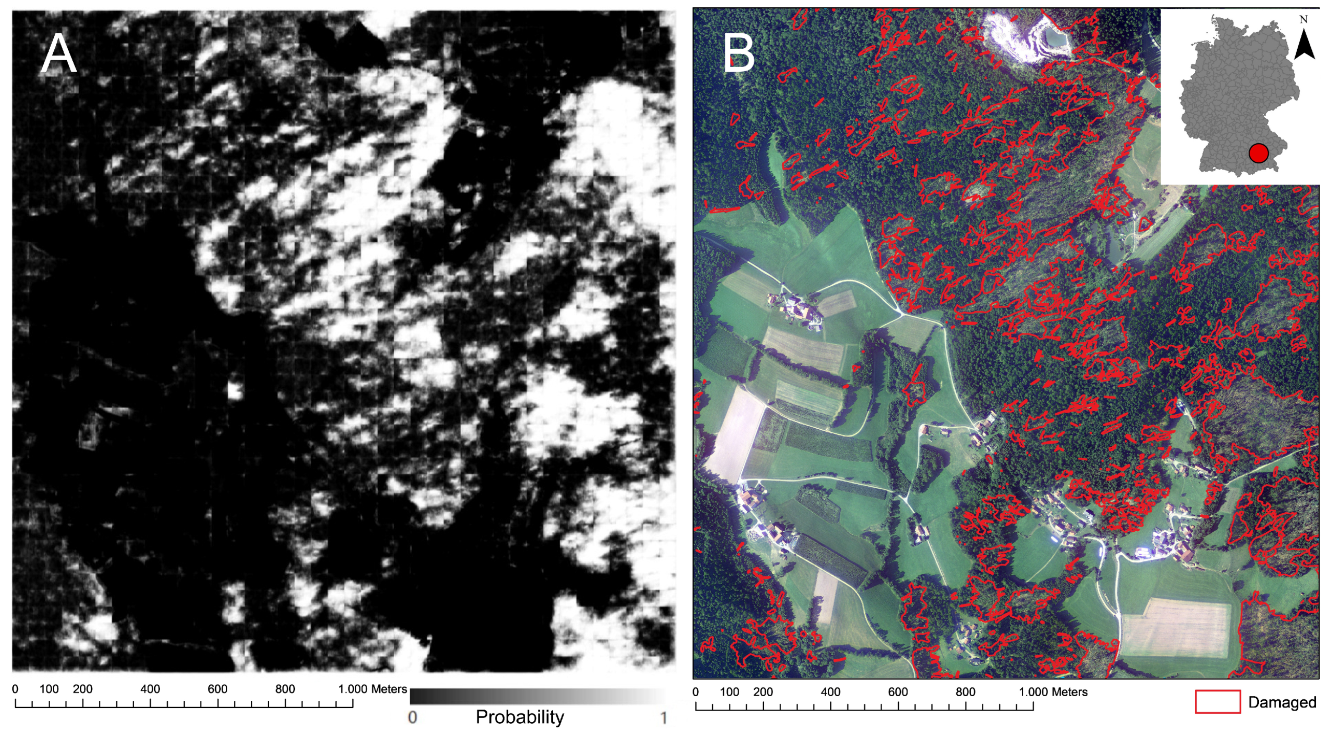
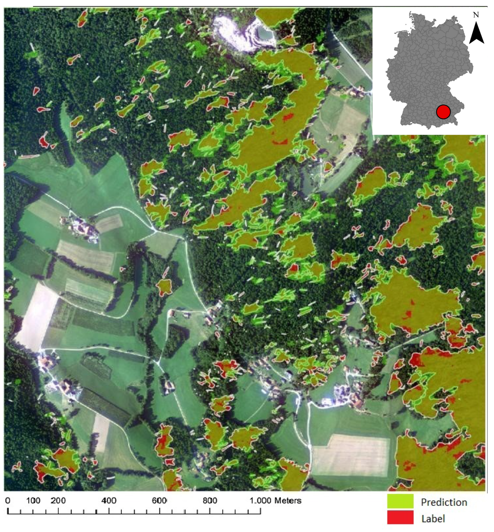
3. Results
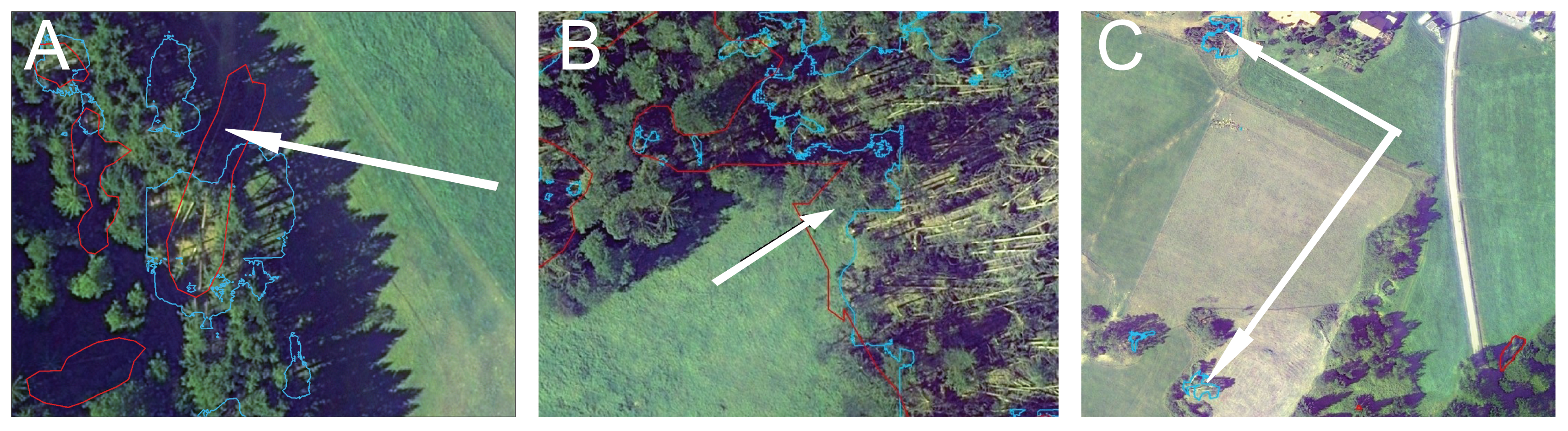
4. Discussion
4.1. Comparison to Other Forest Damage Assessment Approaches
4.2. Limitations of This Study
5. Conclusions and Outlook
Author Contributions
Funding
Acknowledgments
Conflicts of Interest
Abbreviations
| CNN | Convolutional neural network |
| GPU | Graphics processing unit |
| IoU | Intersection over union |
| ReLU | Rectified linear unit |
| SeLU | Scaled exponential linear unit |
References
- Gardiner, B.; Blennow, K.; Carnus, J.M.; Fleischer, P.; Ingemarson, F.; Landmann, G.; Lindner, M.; Marzano, M.; Nicoll, B.; Orazio, C.; et al. Destructive storms in European forests: past and forthcoming impacts. In Destructive Storms in European Forests: Past and Forthcoming Impacts; European Forest Institute: Joensuu, Finland, 2010. [Google Scholar]
- Triebenbacher, C.; Straßer, L.; Lemme, H.; Lobinger, G.; Metzger, J.; Petercord, R. Waldschutzsituation 2017 in Bayern. AFZ-DerWald 2018, 6, 18–21. [Google Scholar]
- Seidl, R.; Thom, D.; Kautz, M.; Martín-Benito, D.; Peltoniemi, M.; Vacchiano, G.; Wild, J.; Ascoli, D.; Petr, M.; Honkaniemi, J.; et al. Forest disturbances under climate change. Nat. Clim. Chang. 2017, 7, 395–402. [Google Scholar] [CrossRef] [PubMed]
- Böhm, P. Sturmschäden in Schwaben von 1950 bis 1980. Allg. Forstz. 1981, 36, 1380. [Google Scholar]
- Mokros, M.; Výbot’ok, J.; Merganic, J.; Hollaus, M.; Barton, I.; Koren, M.; Tomastík, J.; Cernava, J. Early Stage Forest Windthrow Estimation Based on Unmanned Aircraft System Imagery. Forests 2017, 8, 306. [Google Scholar] [CrossRef]
- Nabuurs, G.; Schelhaas, M. Spatial distribution of whole-tree carbon stocks and fluxes across the forests of Europe: where are the options for bio-energy? Biomass Bioenergy 2003, 24, 311–320. [Google Scholar] [CrossRef]
- Einzmann, K.; Immitzer, M.; Böck, S.; Bauer, O.; Schmitt, A.; Atzberger, C. Windthrow Detection in European Forests with Very High-Resolution Optical Data. Forests 2017, 8, 21. [Google Scholar] [CrossRef]
- Tomastík, J.; Saloň, Š.; Piroh, R. Horizontal accuracy and applicability of smartphone GNSS positioning in forests. Forestry 2016, 90, 187–198. [Google Scholar] [CrossRef]
- Wessel, M.; Brandmeier, M.; Tiede, D. Evaluation of Different Machine Learning Algorithms for Scalable Classification of Tree Types and Tree Species Based on Sentinel-2 Data. Remote Sens. 2018, 10, 1419. [Google Scholar] [CrossRef]
- Hościło, A.; Lewandowska, A. Mapping Forest Type and Tree Species on a Regional Scale Using Multi-Temporal Sentinel-2 Data. Remote Sens. 2019, 11, 929. [Google Scholar] [CrossRef]
- Hyyppä, J.; Holopainen, M.; Olsson, H. Laser scanning in forests. Remote Sens. 2012, 4, 2919–2922. [Google Scholar] [CrossRef]
- Anees, A.; Aryal, J. A statistical framework for near-real time detection of beetle infestation in pine forests using MODIS data. IEEE Geosci. Remote Sens. Lett. 2014, 11, 1717–1721. [Google Scholar] [CrossRef]
- Keenan, T.; Darby, B.; Felts, E.; Sonnentag, O.; Friedl, M.; Hufkens, K.; O’Keefe, J.; Klosterman, S.; Munger, J.W.; Toomey, M.; et al. Tracking forest phenology and seasonal physiology using digital repeat photography: a critical assessment. Ecol. Appl. 2014, 24, 1478–1489. [Google Scholar] [CrossRef]
- Jonikavičius, D.; Mozgeris, G. Rapid assessment of wind storm-caused forest damage using satellite images and stand-wise forest inventory data. iFor. Biogeosci. For. 2013, 6, 150–155. [Google Scholar] [CrossRef]
- Baumann, M.; Ozdogan, M.; Wolter, P.T.; Krylov, A.; Vladimirova, N.; Radeloff, V.C. Landsat remote sensing of forest windfall disturbance. Remote Sens. Environ. 2014, 143, 171–179. [Google Scholar] [CrossRef]
- Honkavaara, E.; Litkey, P.; Nurminen, K. Automatic Storm Damage Detection in Forests Using High-Altitude Photogrammetric Imagery. Remote Sens. 2013, 5, 1405–1424. [Google Scholar] [CrossRef]
- Renaud, J.P.; Vega, C.; Durrieu, S.; Lisein, J.; Magnussen, S.; Lejeune, P.; Fournier, M. Stand-level wind damage can be assessed using diachronic photogrammetric canopy height models. Ann. For. Sci. 2017, 74, 74. [Google Scholar] [CrossRef]
- Lecun, Y. Gradient-based learning applied to document recognition. Proc. IEEE. 1998, 86, 2278–2324. [Google Scholar] [CrossRef]
- Ronneberger, O.; Fischer, P.; Brox, T. U-Net: Convolutional Networks for Biomedical Image Segmentation. arXiv 2015, arXiv:1505.04597. [Google Scholar]
- Lu, C.; Chen, H.; Chen, Q.; Law, H.; Xiao, Y.; Tang, C.K. 1-HKUST: Object Detection in ILSVRC 2014. arXiv 2014, arXiv:1409.6155. [Google Scholar]
- Jin, B.; Ye, P.; Zhang, X.; Song, W.; Li, S. Object-Oriented Method Combined with Deep Convolutional Neural Networks for Land-Use-Type Classification of Remote Sensing Images. J. Indian Soc. Remote Sens. 2019, 47, 951–965. [Google Scholar] [CrossRef]
- Rezaee, M.; Mahdianpari, M.; Zhang, Y.; Salehi, B. Deep Convolutional Neural Network for Complex Wetland Classification Using Optical Remote Sensing Imagery. IEEE J. Sel. Top. Appl. Earth Obs. Remote Sens. 2018, 11, 3030–3039. [Google Scholar] [CrossRef]
- Onishi, M.; Ise, T. Automatic classification of trees using a UAV onboard camera and deep learning. arXiv 2018, arXiv:1804.10390. [Google Scholar]
- Freudenberg, M.; Nölke, N.; Agostini, A.; Urban, K.; Wörgötter, F.; Kleinn, C. Large Scale Palm Tree Detection In High Resolution Satellite Images Using U-Net. Remote Sens. 2019, 11, 312. [Google Scholar] [CrossRef]
- Wagner, F.H.; Sanchez, A.; Tarabalka, Y.; Lotte, R.G.; Ferreira, M.P.; Aidar, M.P.M.; Gloor, E.; Phillips, O.L.; Aragão, L.E.O.C. Using the U-net convolutional network to map forest types and disturbance in the Atlantic rainforest with very high resolution images. Remote Sens. Ecol. Conserv. 2019. [Google Scholar] [CrossRef]
- Hafemann, L.G.; Oliveira, L.S.; Cavalin, P. Forest species recognition using deep convolutional neural networks. In Proceedings of the 2014 22nd IEEE International Conference on Pattern Recognition, Stockholm, Sweden, 24–28 August 2014; pp. 1103–1107. [Google Scholar]
- Simonyan, K.; Zisserman, A. Very Deep Convolutional Networks for Large-Scale Image Recognition. arXiv 2014, arXiv:1409.1556. [Google Scholar]
- Frank, C.J.; Redd, D.G.T.M.R. Characterization of human breast biopsy specimens with near-IR Raman spectroscopy. Anal. Chem. 1994, 66, 319–326. [Google Scholar] [CrossRef]
- Chollet, F. Keras. GitHub repository. 2015. Available online: https://github.com/fchollet/keras (accessed on 20 August 2019).
- Jeffrey, D. TensorFlow: A System for Large-Scale Machine Learning; Google Brain: Mountain View, CA, USA, 2015. [Google Scholar]
- Kingma, D.P.; Ba, J. Adam: A Method for Stochastic Optimization. arXiv 2015, arXiv:1412.6980. [Google Scholar]
- Nair, V.; Hinton, G.E. Rectified linear units improve restricted boltzmann machines. In Proceedings of the 27th International Conference on Machine Learning (ICML-10), Haifa, Israel, 21–24 June 2010; pp. 807–814. [Google Scholar]
- Veličković, P. Be nice to your neurons: Initialisation, Normalisation, Regularisation and Optimisation. In Introduction to Deep Learning (COMPGI23); University College London: London, UK, 2017. [Google Scholar]
- Moré, J.J. The Levenberg-Marquardt algorithm: implementation and theory. In Numerical Analysis; Springer: Berlin, Germany, 1978; pp. 105–116. [Google Scholar]
- Wang, W.; Qu, J.J.; Hao, X.; Liu, Y.; Stanturf, J. Post-hurricane forest damage assessment using satellite remote sensing. Agric. For. Meteorol. 2010, 150, 122–132. [Google Scholar] [CrossRef]
- Remelgado, R.; Notarnicola, C.; Sonnenschein, S. Forest damage assessment using SAR and optical data: evaluating the potential for rapid mapping in mountains. EARSeL eProc. 2014, 13, 67–81. [Google Scholar]
- Rüetschi, M.; Small, D.; Waser, L.T. Rapid Detection of Windthrows Using Sentinel-1 C-Band SAR Data. Remote Sens. 2019, 11, 115. [Google Scholar] [CrossRef]
- Eriksson, L.E.B.; Fransson, J.E.S.; Soja, M.J.; Santoro, M. Backscatter signatures of wind-thrown forest in satellite SAR images. In Proceedings of the 2012 IEEE International Geoscience and Remote Sensing Symposium, Munich, Germany, 22–27 July 2012; pp. 6435–6438. [Google Scholar]


| Scenario | Number of Blocks | Number of Filters | Learning Rate | Mean IoU | Accuracy |
|---|---|---|---|---|---|
| 1 | 3 | 64 , 64, 64 | 0.001 | 0.30 | |
| 2 | 4 | 64, 64, 64, 64 | 0.001 | 0.38 | |
| 3 | 5 | 64, 64, 64, 64, 64 | 0.001 | 0.36 | |
| 4 | 6 | 64, 64, 64, 64, 64, 64 | 0.001 | 0.32 | |
| 5 | 4 | 16, 32, 64, 128 | 0.001 | 0.42 | |
| 6 | 4 | 32, 64, 128, 256 | 0.001 | 0.38 | |
| 7 | 4 | 64, 128, 256, 512 | 0.001 | 0.31 | |
| 8 | 4 | 16, 32, 64, 128 | 0.01 | 0.008 | |
| 9 | 4 | 16, 32, 64, 128 | 0.0005 | 0.42 | |
| 10 | 4 | 16, 32, 64, 128 | 0.00001 | 0.39 |
© 2019 by the authors. Licensee MDPI, Basel, Switzerland. This article is an open access article distributed under the terms and conditions of the Creative Commons Attribution (CC BY) license (http://creativecommons.org/licenses/by/4.0/).
Share and Cite
Hamdi, Z.M.; Brandmeier, M.; Straub, C. Forest Damage Assessment Using Deep Learning on High Resolution Remote Sensing Data. Remote Sens. 2019, 11, 1976. https://doi.org/10.3390/rs11171976
Hamdi ZM, Brandmeier M, Straub C. Forest Damage Assessment Using Deep Learning on High Resolution Remote Sensing Data. Remote Sensing. 2019; 11(17):1976. https://doi.org/10.3390/rs11171976
Chicago/Turabian StyleHamdi, Zayd Mahmoud, Melanie Brandmeier, and Christoph Straub. 2019. "Forest Damage Assessment Using Deep Learning on High Resolution Remote Sensing Data" Remote Sensing 11, no. 17: 1976. https://doi.org/10.3390/rs11171976
APA StyleHamdi, Z. M., Brandmeier, M., & Straub, C. (2019). Forest Damage Assessment Using Deep Learning on High Resolution Remote Sensing Data. Remote Sensing, 11(17), 1976. https://doi.org/10.3390/rs11171976