Coupled Higher-Order Tensor Factorization for Hyperspectral and LiDAR Data Fusion and Classification

Abstract

Hyperspectral and light detection and ranging (LiDAR) data fusion and classification has been an active research topic, and intensive studies have been made based on mathematical morphology. However, matrix-based concatenation of morphological features may not be so distinctive, compact, and optimal for classification. In this work, we propose a novel Coupled Higher-Order Tensor Factorization (CHOTF) model for hyperspectral and LiDAR data classification. The innovative contributions of our work are that we model different features as multiple third-order tensors, and we formulate a CHOTF model to jointly factorize those tensors. Firstly, third-order tensors are built based on spectral-spatial features extracted via attribute profiles (APs). Secondly, the CHOTF model is defined to jointly factorize the multiple higher-order tensors. Then, the latent features are generated by mode-n tensor-matrix product based on the shared and unshared factors. Lastly, classification is conducted by using sparse multinomial logistic regression (SMLR). Experimental results, conducted with two popular hyperspectral and LiDAR data sets collected over the University of Houston and the city of Trento, respectively, indicate that the proposed framework outperforms the other methods, i.e., different dimensionality-reduction-based methods, independent third-order tensor factorization based methods, and some recently proposed hyperspectral and LiDAR data fusion and classification methods.

1. Introduction

Remote sensing technologies are vital for Earth observation since they can provide a variety information about the structure (optical or radar), elevation (light detection and ranging, LiDAR), and material content (multispectral or hyperspectral) of the Earth’s surface objects [1]. Typically, individual remote sensing technology is exhausted when dealing with incomplete, inconsistent, or vague image sources, preventing a better understanding of the observed site [2]. Remotely sensed data fusion can be used to achieve a richer description of the scene since it considers the complementarity embedded in multi-source information. Hyperspectral remote sensing image (HSI) is effective in discriminating objects composed of different materials, whereas LiDAR can be used to separate objects with different elevation. However, in the scenario of differentiating objects with the same material or elevation, single technology is usually insufficient for producing reliable results. In this context, hyperspectral and LiDAR data fusion has been exploited to address this issue, which is a hot topic and has been attracted great attention by geoscience and remote sensing society in recent years [3].

New emergent methodological avenues for remotely sensed data fusion have been observed in the last decade, during which period advanced methods drawn from machine learning and signal processing have been gradually advocated by researchers [2]. We will focus on reviewing those methods proposed for hyperspectral and LiDAR data fusion from the following perspectives:

• Mathematical morphology generates multisource spatial features from remotely sensed images, and fuses those features in feature level for image classification by using an independent classifier. For example, attribute profiles (APs) [4,5,6,7,8,9], morphological profiles (MPs) [10,11,12], extinction profiles (EPs) [7,13,14,15,16] were computed on both optical and LiDAR data to extract the multisource features, leading to a fusion of spectral, spatial and elevation information.
• Markov modeling formalizes spatial information and data fusion through global minimum energy concepts, which has been used for remotely sensed data fusion. For example, the work in [17] proposed an edge-constrained Markov random field method for accurate land cover classification over urban areas using hyperspectral and LiDAR data.
• Sparse representation conducts data fusion by minimizing the signal-to-reconstruction error with a predefined dictionary and a sparse-inducing constraint. For example, in [18], a method of fusing hyperspectral and LiDAR data for landscape visual quality assessment was presented, where the relationship between physical features and human landscape preferences was learned using least absolute shrinkage and selection operator regression. Further, joint sparse representation [19] and sparse low-rank [20] techniques were exploited for the fusion and classification of hyperspectral and LiDAR data.
• Ensemble learning conducts data fusion in decision level by combining results from many weak learners based on multisource features. For example, multiple fuzzy classifier system was studied for hyperspectral and LiDAR data fusion [21,22]. In addition, the work in [12] used a random forest classifier to produce multiple classification results based on multiple features, and majority voting was then used to fuse the results.
• Multiple kernel learning performs data fusion in implicit high-dimensional feature representations. For example, multiple kernel learning [23,24] and composite kernel [16,25] were used to extract heterogeneous information from hyperspectral and LiDAR data.
• Manifold learning serves as a framework for low-dimensional feature extraction through graph embedding, where data fusion coupled with dimensionality reduction can be conducted by fusing the Laplacian matrices computed for multisource data. For example, generalized graph-based method [10], kernel local Fisher discriminant analysis [25], discriminative graph-based method [11], and orthogonal total variation component analysis [14] were used to extract low-dimensional features for hyperspectral and LiDAR data fusion.
• Image segmentation is used to generate image objects which are then used for classification based on hyperspectral and LiDAR data [26,27].
• Hash learning is used to extract compact binary features which are then used for HSI classification [28].
• Deep Learning is used to extract the informative features from hyperspectral and LiDAR data in a hierarchical feature learning manner [7,8,13,15,29,30].

Although elegant fusion and classification performances have been obtained by using these methods, none of the current subpixel, pixel, feature, or decision level fusion methods are capable of breaking the limitations of standard flat-view matrix based models. On the one hand, formulating the multisource features as a long vector or high-dimensional matrix will inevitably cause the curse of dimensionality issue since the available training samples are very limited. On the other hand, the matrix-based concatenation of multisource features may not be so distinctive, compact, and optimal for the classification purpose.

Tensor is a generalization of vector or matrix to higher dimension, and the order of a tensor is the number of its dimension. Usually, the first-order array is a vector, the second-order array is a matrix, and the third-order array is a tensor. Higher-order tensors possess properties that are not present on the matrix level. In terms of HSI, vector- or matrix-based representation destroys the inherent spatial and spectral structure which can offer a physical interpretation of how spatial information and spectral bands contribute to the classification outcome [31]. Benefiting from the power of tensorization, data analysis techniques using tensor decompositions are shown to have great flexibility in the choice of constraints which match data properties and extract more general latent components than vector- or matrix-based methods.

Tensor decomposition opens up new possibilities for remote sensing image processing, as it can alleviate or even break the curse of dimensionality that occurs when working with high-dimensional features [32]. In addition, natural images are usually generated by the interaction of multiple factors related to scene structure, illumination and imaging [33]. Recently, tensor decomposition has shown great potentials for HSI classification [34,35,36], denosing [37], dimensionality reduction [38], hyperspectral and multispectral image fusion [39], target detection [40,41], spectral unmixing [42], etc. However, previous tensor factorization related studies rarely exploited hyperspectral and LiDAR data fusion and classification.

Data fusion concerns the joint analysis of an ensemble of data sets, such as multiple views of a particular phenomenon, where some parts of the scene may be visible in only one or a few data sets [43]. Tensor decomposition, e.g., canonical polyadic decomposition, can represent any Nth-order tensor as a linear combination of rank-one tensors, which is related to data fusion since the multiple data sources are often heterogeneous in the form of higher-order tensors [44]. In this context, tensor decomposition can extract the shared components between data sources with those rank-one tensors, and the revealed structures of tensor decomposition may further contribute to interpretability, separability, robustness, and uniqueness in feature representation [45].

In addition, this decomposition can be enhanced by coupled tensor factorization, where the different factorizations are coupled with each other by indicating which factors should be shared and unshared between data sources. In general, the advantages of using the coupled tensor factorization are [46]: (1) Coupled analysis can enhance knowledge discovery in terms of missing data; (2) Coupled analysis can preserve uniqueness properties in multiple data sets; (3) Coupled analysis provides robustness in the case of noisy data sets. In this context, a structured data fusion (SDF) framework was presented recently serving as a general prototype of knowledge discovery between multiple data sources [47]. SDF framework can fit many applications including social network mining, documents classification, link prediction, signal processing, etc.

In this work, we propose a novel coupled high-order tensor factorization (CHOTF) model for hyperspectral and LiDAR data fusion and classification based on morphological features. Firstly, third-order tensors are generated based on the spectral-spatial features extracted via attribute profiles (APs). Secondly, a CHOTF model is defined to obtain the shared and unshared factors. Then, the latent features are generated by mode-n tensor-matrix product based on the shared factors, which are then used to yield the latent features. Finally, a sparse multinomial logistic regression (SMLR) classifier is used for classification with the extracted features. The proposed framework is a fundamental paradigm that can well match data properties and extract more latent features than conventional matrix-based methods.

It should be noted that recent study in [34] is related to our work. There are, however, three major conceptual differences. First, we focus on hyperspectral and LiDAR data fusion by using third-order tensor factorization based on morphological features, whereas in [34], morphological feature extraction and tensor discriminant analysis were integrated for HSI classification. Second, our work models the extracted spectral-spatial features as third-order tensors, whereas the work [34] rearranged the features into second-order tensors, which actually is still in flat-view matrix style. Third, we conduct coupled tensor factorization based on multiple tensors, whereas the work [34] actually belongs to matrix factorization. In this context, the main contributions of this paper to the literature are as follows:

• We propose a novel coupled high-order tensor factorization model for hyperspectral and LiDAR data fusion and classification, which is unique compared with regard to previously proposed approaches in this area. Note that, this is the first time of exploiting tensor factorization for hyperspectral and LiDAR data fusion.
• We propose to represent HSI, HSI-derived EMAPs, and LiDAR-derived APs as third-order tensors, and the shared and unshared factors are produced by using coupled tensor factorization.
• Last but not least, only training samples are fed into the model for factorizing, and feature projection is achieved by using model-n tensor-matrix product based on shared factors and the test samples.

2. Materials and Methods

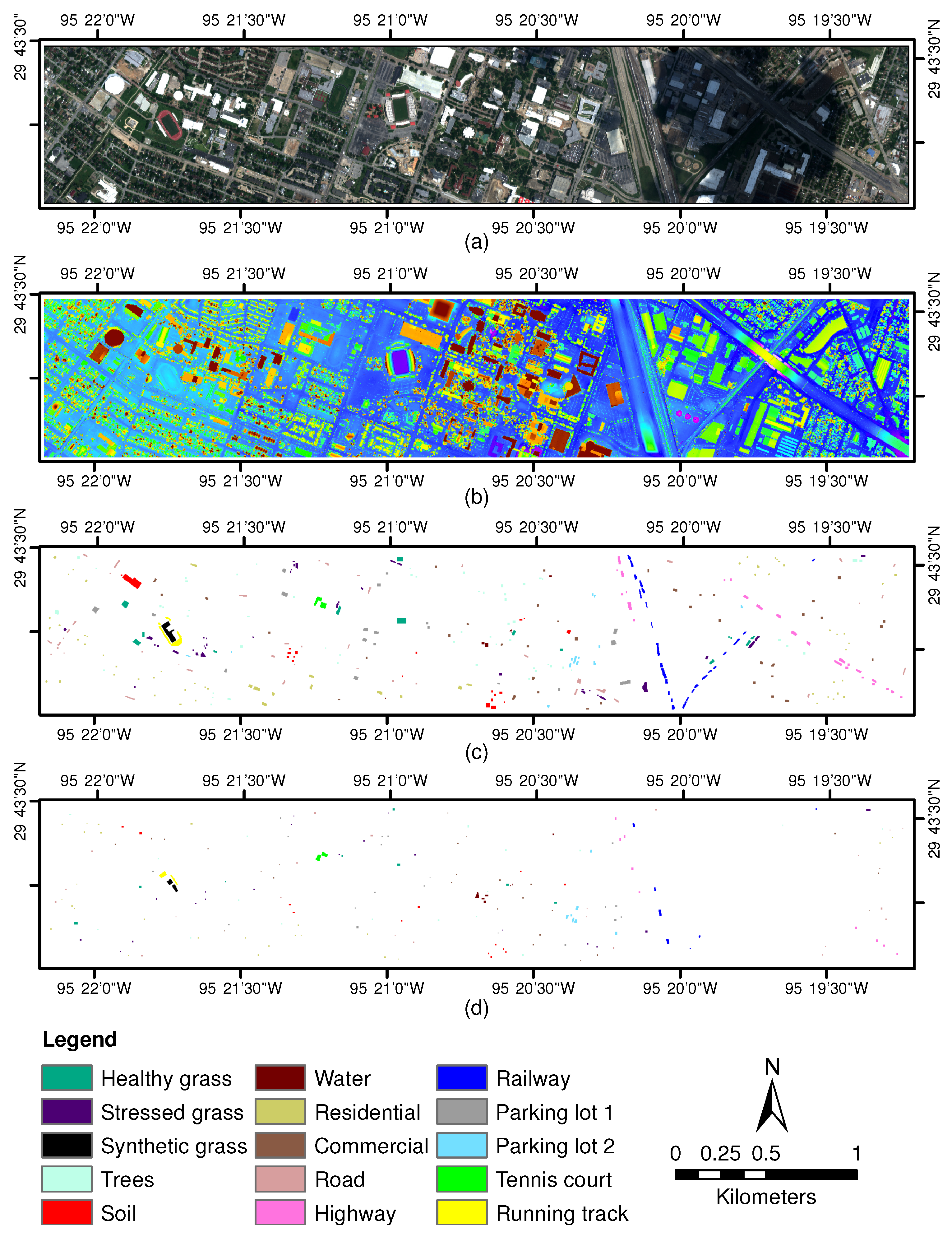
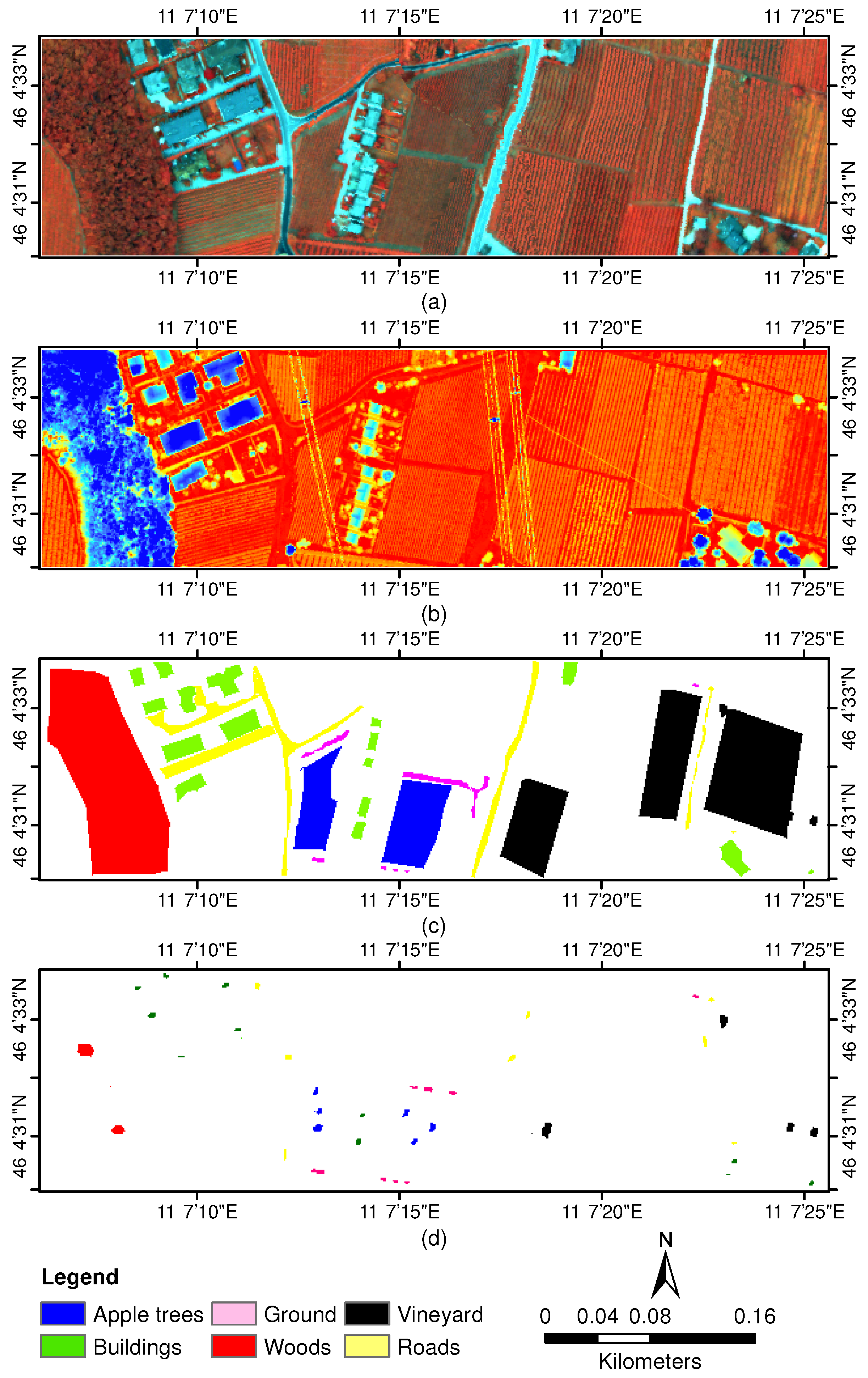
2.1. Validation Test Sites

The first University of Houston data sets used in the experiments were distributed by the 2013 IEEE GRSS Data Fusion Contest (Available online: http://hyperspectral.ee.uh.edu/?page_id=459). The data sets include a HSI and a LiDAR-derived digital surface model (DSM), both at the same spatial resolution (2.5 m). The HSI has 144 bands in the 380–1050 nm spectral region. The corresponding co-registered DSM represents the elevation in meters above sea level (per the Geoid 2012A model). The data sets were acquired by the National Science Foundation (NSF)-funded Center for Airborne Laser Mapping (NCALM) over the University of Houston campus and its neighboring area. The HSI was acquired on 23 June 2012 between 17:37:10 and 17:39:50 UTC. The average height of the sensor above ground was 5500 feet. The LiDAR data was acquired on 22 June 2012, between 14:37:55 and 15:38:10 UTC. The average height of the sensor above ground was 2000 feet. For illustrative purpose, Figure 1a shows a false color composition of the HSI. Figure 1b exhibits the LiDAR-derived DSM. Figure 1c plots the ground truth available for the Houston data, which comprises 15 mutually exclusive classes and is used for validation. Finally, Figure 1d gives the training set used in our experiments.

Table 1. Ground-truth classes and corresponding train- and test-set sizes for University of Houston data sets.

Class	#Samples
	Train	Test
Healthy grass	198	1053
Stressed grass	190	1064
Synthetic grass	192	505
Trees	188	1056
Soil	186	1056
Water	182	143
Residential	196	1072
Commercial	191	1053
Road	193	1059
Highway	191	1036
Railway	181	1054
Parking lot 1	192	1041
Parking lot 2	184	285
Tennis court	181	247
Running track	187	473
Total	2832	12197

details the classes and the number of available samples for training and test.

The second Trento data sets used in the experiments were captured over a rural area south of the city of Trento, Italy. The hyperspectral data was captured by the AISA Eagle sensor, with 63 bands ranging from 402.89 to 989.09 nm, and the spectral resolution is 9.2 nm. The LiDAR DSM data was acquired by the Optech ALTM 3100EA sensor. This data sets have 600 × 166 pixels, with the spatial resolution of 1 m. Six classes of interests were extracted, including building, woods, apple trees, roads, vineyard, and ground. For illustrative purpose, Figure 2a shows a false color composition of the HSI. Figure 2b exhibits the LiDAR-derived DSM. Figure 2c plots the ground truth available for this data sets, which comprises 6 mutually exclusive classes and is used for validation. Finally, Figure 2d gives the training set used in our experiments. Note that the reported coordinates in this figure have been offset for privacy.

Table 2. Ground-truth classes and corresponding train- and test-set sizes for Trento data sets.

Class	#Samples
	Train	Test
Apple trees	129	4034
Buildings	125	2903
Ground	105	479
Woods	154	9123
Vineyard	184	10501
Roads	122	3174
Total	819	30214

reports the classes and the number of available samples for training and test.

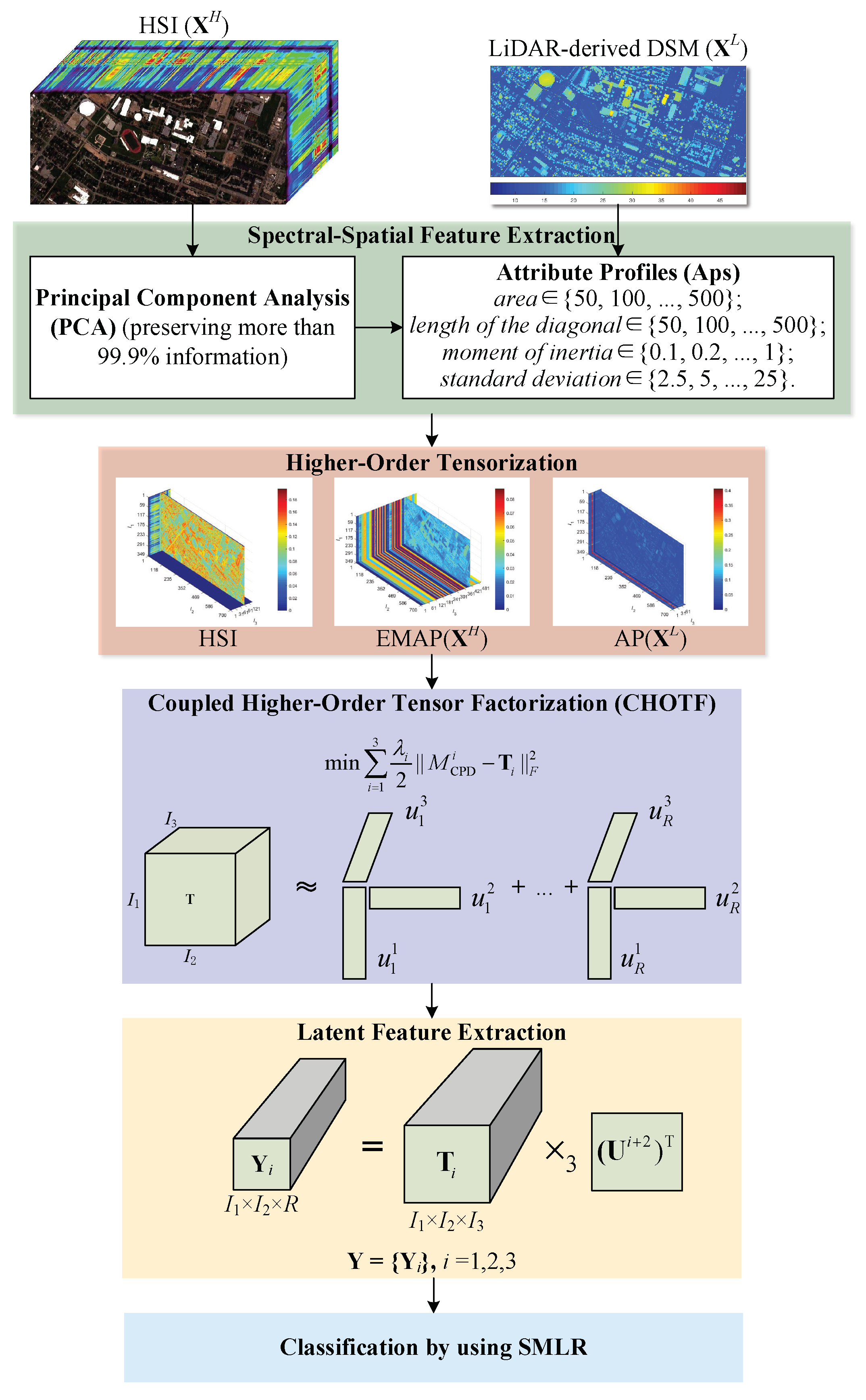
2.2. Proposed Methodology

First of all, we introduce the notations that will be adopted throughout this paper. Let $\mathbf{X}=[{\mathbf{x}}_1,\dots ,{\mathbf{x}}_N]\in {\mathbb{R}}^{B\times N}$ be a remote sensing data set with a B-dimensional signal for each pixel x${}_i={[x_1,\dots ,x_B]}^{\mathrm{T}}$, $i\in 1,\dots ,N$. Let $\mathbf{T}\in {\mathbb{R}}^{I_1\times I_2\times \dots \times I_m}$ be a m-order tensor. Let $\mathbf{Y}=[{\mathbf{y}}_1,\dots ,{\mathbf{y}}_N]\in {\mathbb{R}}^{M\times N}$ ($M\ll B$) be the latent features extracted from X. We denote by X${}^H$ and X${}^L$ the HSI and the LiDAR data, respectively.

The proposed framework consists of four major steps: (1) extract spectral-spatial features via APs and generate higher-order tensors based on the features; (2) define a coupled higher-order tensor factorization model; (3) generate more latent features via mode-n tensor-matrix product; (4) conduct classification by using SMLR. The flowchart is shown in Figure 3 with more details given as follows.

2.2.1. Spectral-Spatial Features Extraction via APs

Morphological profiles (MPs) [48] concatenates multi-scale decompositions of an image carried out with a series of opening and closing transformations based on the geodesic reconstruction. Extended morphological profile (EMP) [49] is the concatenation of the MPs computed on each of the principal components (PCs) extracted from the data. Whereas, extended multi-morphological profile (EMMP) is the concatenation of the EMPs in terms of different structure element (SE). MPs, EMP, and EMMP can be formulated as

$$\begin{array}{c}\mathrm{MP}\left(\mathbf{X}\right)=\{{\varphi }_1\left(\mathbf{X}\right),\dots ,{\varphi }_{\lambda }\left(\mathbf{X}\right),\dots ,{\varphi }_l\left(\mathbf{X}\right),\mathbf{X},{\gamma }_1\left(\mathbf{X}\right),\dots ,{\gamma }_{\lambda }\left(\mathbf{X}\right),\dots ,{\gamma }_l\left(\mathbf{X}\right)\}\hfill \\ \mathrm{EMP}\left(\mathbf{X}\right)=\{\mathrm{MP}\left({\mathrm{PC}}_1\right),\mathrm{MP}\left({\mathrm{PC}}_2\right),\dots ,\mathrm{MP}\left({\mathrm{PC}}_{\mathit{c}}\right)\}\hfill \\ \mathrm{EMMP}\left(\mathbf{X}\right)=\{{\mathrm{EMP}}_1,{\mathrm{EMP}}_2,\dots ,{\mathrm{EMP}}_{\mathit{a}}\},\hfill \end{array}$$

(1)

where $\varphi$ is closing operator, $\gamma$ is opening operator, $\lambda =1,\dots ,l$ denotes the size of a specific SE, c is the number of PCs, and a is the number of different SEs, i.e., disk, diamond, and square.

To overcome the drawbacks of MPs, APs [50] was proposed. Analogously to the definitions of EMPs and EMMPs, extended attribute profile (EAP) and extended multi-attribute profile (EMAP) take the forms [51]

$$\begin{array}{c}\mathrm{EAP}\left(\mathbf{X}\right)=\{\mathrm{AP}\left({\mathrm{PC}}_1\right),\mathrm{AP}\left({\mathrm{PC}}_2\right),\dots ,\mathrm{AP}\left({\mathrm{PC}}_{\mathit{c}}\right)\}\hfill \\ \mathrm{EMAP}\left(\mathbf{X}\right)=\{{\mathrm{EAP}}_1,{\mathrm{EAP}}_2,\dots ,{\mathrm{EAP}}_{\mathit{a}}\}.\hfill \end{array}$$

(2)

Here a denotes the number of different attributes.

In this paper, we chose to use APs to extract the spectral-spatial features based on HSI and LiDAR data, where the attributes are area, length of the diagonal, moment of inertia, and standard deviation. Before applying those filters, APs adopts a Max-tree structure to represent the connected components of the image, where each node reports the values of different attributes [50]. In this context, a total of $ac(2l+1)$ images are concatenated in EMAPs derived from HSI, and the number is $a(2l+1)$ for LiDAR since it only has one band.

2.2.2. Higher-Order Tensor Representation

As we mentioned before, mathematical morphology has some limitations for hyperspectral and LiDAR data classification. However, tensor factorization has great flexibility in the choice of constraints which can preserve data structures and extract more latent features [43], which inspires us to conduct tensorization for APs, with the aim of producing more powerful features for classification.

To this end, we model the extracted spectral-spatial features as third-order tensors in a very natural way, i.e., $\mathbf{T}\in {\mathbb{R}}^{I_1\times I_2\times I_3}$, where $I_1$ is image height, $I_2$ is image width, and $I_3$ is image or feature dimension. Take the tensorization of HSI-derived EMAPs as an example, we first obtain c PCs by preserving more than 99.9% information. Then, we choose to use four types of attributes with predefined parameters to model the spatial information for each PC. Finally, we rearrange the obtained features into third-order tensors as aforementioned. In this context, we can obtain a tensor with $I_1\times I_2\times 4c(2l+1)$ [the number of parameters for each attribute is equally set to l, see Equation (2)]. Traditional methods treat the features as matrices, which may lose the structural correlations between pixels.

Similar tensorization can be applied to the original HSI and LiDAR-derived APs. We denote by ${\mathbf{T}}_1$ ($I_1\times I_2\times B$), ${\mathbf{T}}_2$ [$I_1\times I_2\times 4c(2l+1)$], and ${\mathbf{T}}_3$ [$I_1\times I_2\times 4(2l+1)$] the tensors for original HSI, HSI-derived EMAPs, and LiDAR-derived APs, respectively. Parts of Figure 3 visually depicts this tensorization.

2.2.3. Coupled Higher-Order Tensor Factorization

Generally, a third-order tensor $\mathbf{T}\in {\mathbb{R}}^{I_1\times I_2\times I_3}$ building from image or features can be factorized by a canonical polyadic decomposition (CPD) model taking the form [52]

$$\mathbf{T}\approx M_{\mathrm{CPD}}({\mathbf{U}}^1,{\mathbf{U}}^2,{\mathbf{U}}^3)=\sum _{r=1}^R{\mathbf{u}}_r^1\otimes {\mathbf{u}}_r^2\otimes {\mathbf{u}}_r^3,$$

(3)

where ${\mathbf{U}}^n\in {\mathbb{R}}^{I_n\times R}$ is the factor matrix, ${\mathbf{u}}_r^n$ is the column of ${\mathbf{U}}^n$, and R is the rank-one term. Parts of Figure 3 graphically illustrates this decomposition.

Inspired by the SDF framework, we propose to fuse hyperspectral and LiDAR data by formulating a CHOTF model, which takes the form

$$\begin{array}{c}\hfill \underset{{\mathbf{U}}^1,{\mathbf{U}}^2,{\mathbf{U}}^3,{\mathbf{U}}^4,{\mathbf{U}}^5}{min}\frac{{\lambda }_1}{2}{∥M_{\mathrm{CPD}}^1({\mathbf{U}}^1,{\mathbf{U}}^2,{\mathbf{U}}^3)-{\mathbf{T}}_1∥}_F^2\\ \hfill +\frac{{\lambda }_2}{2}{∥M_{\mathrm{CPD}}^2({\mathbf{U}}^1,{\mathbf{U}}^2,{\mathbf{U}}^4)-{\mathbf{T}}_2∥}_F^2\\ \hfill +\frac{{\lambda }_3}{2}{∥M_{\mathrm{CPD}}^3({\mathbf{U}}^1,{\mathbf{U}}^2,{\mathbf{U}}^5)-{\mathbf{T}}_3∥}_F^2\\ \hfill +\frac{{\lambda }_4}{2}\left({∥{\mathbf{U}}^1∥}_F^2+{∥{\mathbf{U}}^2∥}_F^2+{∥{\mathbf{U}}^3∥}_F^2+{∥{\mathbf{U}}^4∥}_F^2+{∥{\mathbf{U}}^5∥}_F^2\right),\end{array}$$

(4)

where ${∥·∥}_F^2$ stands for the Frobenius norm of the input, and the shared factors are height factor ${\mathbf{U}}^1\in {\mathbb{R}}^{I_1\times R}$ (i.e., the first dimension of ${\mathbf{T}}_1$) and width factor ${\mathbf{U}}^2\in {\mathbb{R}}^{I_2\times R}$ (i.e., the second dimension of ${\mathbf{T}}_1$), whereas ${\mathbf{U}}^3\in {\mathbb{R}}^{B\times R}$ denotes the band factor (i.e., the third dimension of ${\mathbf{T}}_1$). In addition, ${\mathbf{U}}^4\in {\mathbb{R}}^{4c(2l+1)\times R}$ and ${\mathbf{U}}^5\in {\mathbb{R}}^{4(2l+1)\times R}$ denote the spectral-spatial factors (i.e., the third dimension of ${\mathbf{T}}_2$ and ${\mathbf{T}}_3$), respectively, for HSI-derived EMAPs and LiDAR-derived APs. We also add a $L_2$ regularization term to the objective function to prevent overfitting. In the equation, ${\lambda }_1$, ${\lambda }_2$, and ${\lambda }_3$ are the weight parameters controlling the tradeoff between coupled factorization of HSI (the first part), HSI-derived EMAPs (the second part), and LiDAR-derived APs (the third part). Whereas, the last term weighted by ${\lambda }_4$ imposes some sparsity on the decomposition. It’s worth noting that different dimensions $I_1$, $I_2$, and $I_3$ may affect the relative weights of different term. The above Equation (4) is solved by using a nonlinear least squares (NLS) algorithm.

2.2.4. Latent Feature Extraction

We then move our focus to extract the latent features based on the factorizations of CHOTF. The latent features can be obtained by mode-n tensor-matrix product

$$\begin{array}{cc}\hfill {\mathbf{Y}}_1& ={\mathbf{T}}_1{\times }_3{\left({\mathbf{U}}^3\right)}^{\mathrm{T}}\hfill \\ \hfill {\mathbf{Y}}_2& ={\mathbf{T}}_2{\times }_3{\left({\mathbf{U}}^4\right)}^{\mathrm{T}}\hfill \\ \hfill {\mathbf{Y}}_3& ={\mathbf{T}}_3{\times }_3{\left({\mathbf{U}}^5\right)}^{\mathrm{T}},\hfill \end{array}$$

(5)

where symbol “${\times }_3$” denotes the 3-mode product of tensor ${\mathbf{T}}_i$ ($i=1,2,3$) with the corresponding fraction matrix ${\mathbf{U}}^{i+2}$ along the mode-3.

Finally, the extracted latent features Y are rearranged back into matrix representations with dimension $R\times N$, where $N=I_1\times I_2$ denotes the total number of pixels in the image. It’s worth noting that the latent features can be extracted based on ${\mathbf{T}}_1$, ${\mathbf{T}}_2$, and ${\mathbf{T}}_3$, which respectively resulting in ${\mathbf{Y}}_1$, ${\mathbf{Y}}_2$, and ${\mathbf{Y}}_3$. These features are then fused by matrix-concatenation, i.e., $\mathbf{Y}=\{{\mathbf{Y}}_1,{\mathbf{Y}}_2,{\mathbf{Y}}_3\}$, for further classification.

2.2.5. Classification By Using SMLR

In the last stage, the fused features are then embedded into a sparse multinomial logistic regression (SMLR) [53] model for training and prediction. We adopt the Multinomial Logistic Regression via a Variable Splitting and Augmented Lagrangian (LORSAL) algorithm to optimize the model since LORSAL [54] has yielded efficient and powerful performances for HSI classification in recent years  [55,56,57,58,59,60]. In addition, LORSAL has high flexibility in conjunction with other disciplines, such as the Markov Random Field (MRF) that models spatial information; the Gaussian radial basis function (RBF) kernel that maps the input features into more separable space. However, we only conduct a linear SMLR without using MRF for the sake of evaluating the discriminant performance of the derived features without any other disturbances. Algorithm 1 summarizes the proposed framework.

Algorithm 1 Coupled higher-order tensor factorization for hyperspectral and LiDAR data fusion and classification.

1: Input:${\mathbf{X}}^H$ and ${\mathbf{X}}^L$   2: Output: Y 3: Spectral-spatial feature extraction via APs as Equation (2): EMAP(X${}^H$) and AP(X${}^L$) 4: Tensorization for APs: ${\mathbf{T}}_1=M_{\mathrm{CPD}}^1({\mathbf{U}}^1,{\mathbf{U}}^2,{\mathbf{U}}^3)$ for original HSI ${\mathbf{T}}_2=M_{\mathrm{CPD}}^2({\mathbf{U}}^1,{\mathbf{U}}^2,{\mathbf{U}}^4)$ for HSI-derived EMAPs ${\mathbf{T}}_3=M_{\mathrm{CPD}}^3({\mathbf{U}}^1,{\mathbf{U}}^2,{\mathbf{U}}^5)$ for LiDAR-derived APs 5: Coupled higher-order tensor factorization using Equation (4):   ${\mathbf{U}}^1,{\mathbf{U}}^2,{\mathbf{U}}^3,{\mathbf{U}}^4,{\mathbf{U}}^5$   6: Latent feature extraction using Equation (5): ${\mathbf{Y}}_i={\mathbf{T}}_i{\times }_3{\left({\mathbf{U}}^{i+2}\right)}^{\mathrm{T}},i=1,2,3$   7: Feature fusion via matrix-concatenation:   $\mathbf{Y}=\{{\mathbf{Y}}_1,{\mathbf{Y}}_2,{\mathbf{Y}}_3\}$   8: Classification using SMLR optimized by LORSAL based on the fused features Y.

3. Results

3.1. Experimental Settings

The corresponding parameter settings and notations adopted in our experiments are:

• For building EMAP(X${}^H$) and AP(X${}^L$), the four types of attributes are set as area∈{50, 100, ..., 500}; length of the diagonal∈{50, 100, ..., 500}; moment of inertia∈{0.1, 0.2, ..., 1}; standard deviation∈{2.5, 5, ..., 25}. Especially, when using Principal Component Analysis (PCA) to build EMAP(X${}^H$), the features extracted by PCA preserving more than 99.9% information according to the cumulative variance, i.e., 6 PCs for University of Houston data sets, and 8 PCs for Trento data sets.
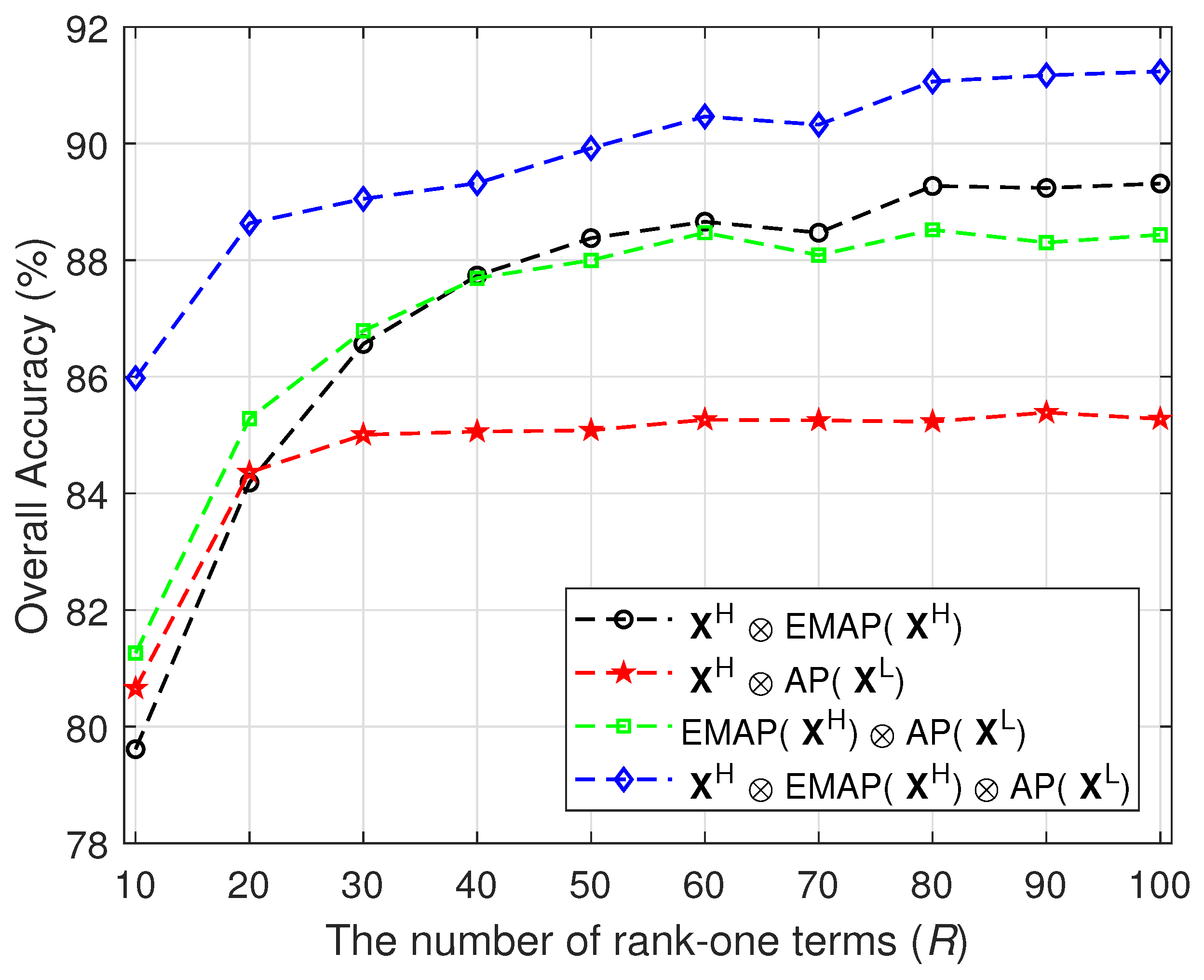
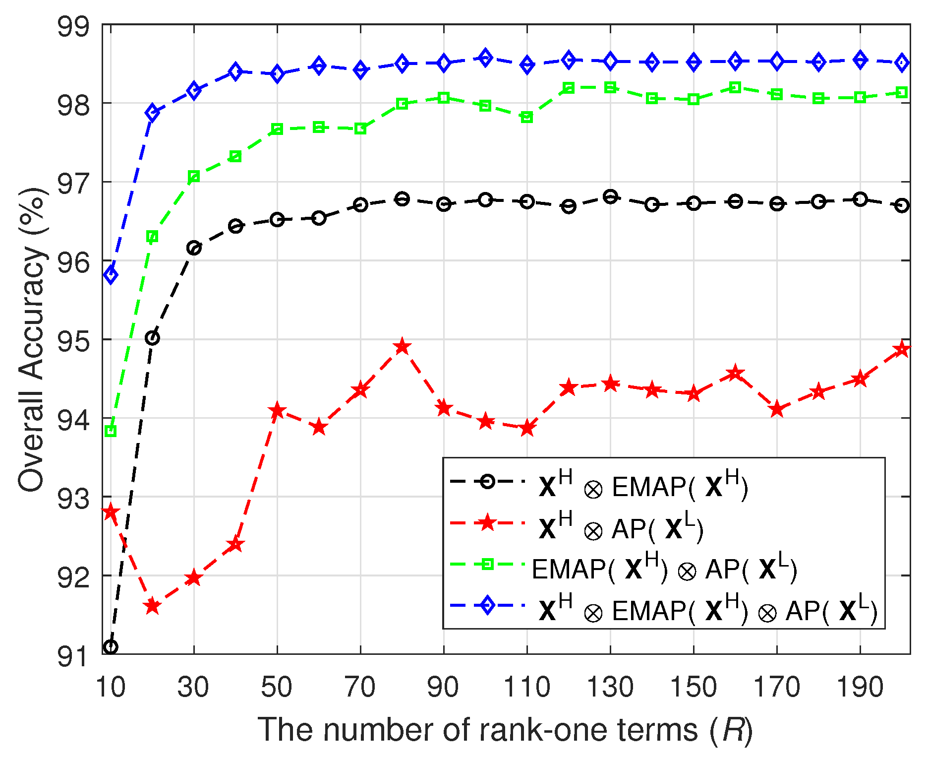
• For the proposed method, we experimentally set ${\lambda }_1={\lambda }_2={\lambda }_3=1$, and ${\lambda }_4=0.01$. Although this parameter setting may not be optimal, it has produced good results in our experiments. As for the rank-one term R, we carefully optimized it in the experiments for different data sets.
• The individual features considered in this work include: the original HSI (X${}^H$), the EMAP built on X${}^H$ [EMAP(X${}^H$)], and the AP built on X${}^L$ [AP(X${}^L$)]. We denote by “A⊗B” the proposed CHOTF-based fusion based on different features A and B.
• In the comparison with different dimensionality reduction (DR) methods, we include PCA, Linear Graph Embedding (LGE), Locality Preserving Projections (LPP), Linear Discriminant Analysis (LDA), and Marginal Fisher Analysis (MFA). Different DR methods are applied on each individual features, and each extracted features preserving more than 99.9% information, then the extracted features are stacked together for classification.
• In the comparison with independent third-order tensor factorization methods, we include canonical polyadic decomposition (CPD) [52], decomposition in multilinear rank-($L_R,L_R,1$) terms (LL1) [61], multilinear singular value decomposition (MLSVD) [62], low multilinear rank approximation (LMLRA) [52], and block term decomposition (BTD) [52]. Note that we fixed the variables instead of random initialization for different tensor-based methods.
• In the comparison with other hyperspectral and LiDAR data fusion methods, we include generalized graph-based fusion (GGF) [10], EPs based on CNN (EP+CNN) [13], deep fusion [7], two-branch CNN [29], three-stream CNN [15], hyperspectral multisensor composite kernels (HyMCKs) [16], higher order discriminant analysis (HODA) [63], local tensor discriminant analysis (LTDA) [34]. Note that, we fed our extracted APs into GGF, HODA, and LTDA for feature extraction, whereas for other methods, we directly reported their accuracies. This comparison is fair since the same training and test samples were used in those considered methods.
• In the comparison with different classifiers, we include random forest (RF) [64], support vector machine (SVM) implemented by LIBSVM [65], subspace projection based multinomial logistic regression (MLR) algorithm (MLRsub) [66], MLR optimized via a variable splitting and augmented Lagrangian algorithm and on a multilevel logistic prior (LORSAL-MLL) [54], and generalized composite kernel framework using multinomial logistic regression (MLR-GCK) [67]. In our paper, we adopt a SMLR classifier to produce the final classification map. SMLR model is optimized by using LORSAL, where the regularization parameter is set to $1\times {10}^{-5}$ and the number of iterations is set to 100.
• The classification results are quantitatively evaluated by measuring the overall accuracy (OA), the average accuracy (AA), the individual class accuracy, and the Kappa statistic ($\kappa$). Note that we were neither intend to select the training samples from ground-truth nor try to split the ground-truth into training and test sets. Whereas, we directly used the training set to train our classifier which was then directly applied to the test set for validation.
• Finally, it should be noted that all the implementations were carried out using Matlab R2017b in a desktop PC equipped with an Intel Xeon E3 CPU (at 3.4 GHz) and 32 GB of RAM.

3.2. Experiments With University of Houston Data Sets

3.2.1. Experiment 1—Parameter Sensitiveness Analysis

In the first experiment, we evaluate the impacts of rank-one term (R) on classification accuracy of different CHOTF-based fusion methods. As shown in Figure 4, the OAs increase as R also increase in different cases. When $R\ge 80$, the OAs for ${\mathbf{X}}^H$⊗ AP(${\mathbf{X}}^L$) and ${\mathbf{X}}^H$⊗ EMAP(${\mathbf{X}}^H$) ⊗ AP(${\mathbf{X}}^L$) remains stable. Whereas for the other two methods, the OAs gradually increase with the increase of R. Therefore, R is experimentally set to 100 in this scene. Another observation is that ${\mathbf{X}}^H$⊗ EMAP(${\mathbf{X}}^H$) ⊗ AP(${\mathbf{X}}^L$) always produces the highest accuracy in different cases.

3.2.2. Experiment 2—Comparison with DR-Based Methods

In the third experiment, we compare the proposed CHOTF-based fusion method [based on ${\mathbf{X}}^H$ ⊗ EMAP(${\mathbf{X}}^H$) ⊗ AP(${\mathbf{X}}^L$)] with different dimensionality reduction methods, i.e., PCA, LGE, LPP, LDA, and MFA. As reported in

Table 3. Overall (OA), average (AA) and individual class accuracies (%), and kappa statistic ($\kappa$) obtained by SMLR based on DR-derived features and CHOTF-derived features for the University of Houston data sets.

Class	PCA	LGE	LPP	LDA	MFA	CHOTF
Healthy grass	83.10	82.81	83.10	83.00	83.10	83.00
Stressed grass	97.18	84.40	85.06	98.68	84.87	95.68
Synthetic grass	100.00	100.00	100.00	100.00	100.00	100.00
Trees	93.37	95.45	84.09	90.06	88.54	95.83
Soil	99.91	100.00	100.00	99.91	100.00	99.91
Water	100.00	99.30	99.30	95.10	98.60	95.10
Residential	95.62	88.06	82.93	83.40	87.87	89.93
Commercial	55.94	75.69	57.64	54.13	60.21	82.43
Road	95.47	94.05	93.96	94.33	97.26	94.43
Highway	57.24	59.07	67.76	90.54	68.15	68.24
Railway	99.05	93.93	98.96	85.96	99.72	99.15
Parking lot 1	93.28	97.89	85.49	91.45	85.98	96.06
Parking lot 2	80.00	83.16	78.25	78.60	74.74	80.70
Tennis court	100.00	100.00	100.00	99.60	100.00	99.60
Running track	100.00	100.00	100.00	100.00	100.00	98.94
Average accuracy	90.01	90.25	87.77	89.65	88.60	91.93
Overall accuracy	88.37	88.51	85.59	88.32	86.96	91.24
$\kappa$ statistic	0.874	0.875	0.844	0.873	0.858	0.905

, CHOTF also outperforms the other DR-based methods with 3–6% improvements of OA. For AA and $\kappa$, the improvements of CHOTF are 1–2% and 0.03–0.06%, respectively, compared to other DR-based methods. Classification results can also be visually inspected according to Figure 5. The cloud-shadow region is classified very different due to the fact that the training samples are not available in this region [see Figure 1d] and the spectral radiance of objects is distorted due to darkening effects. We should note that the reported accuracies are only related to the ground-truth pixels, which may be not in accordance with the visual inspection of classification maps since we also provide the labels for the remaining pixels in the whole image scene. For example, most of the pixels in the cloud-shadow region are misclassified to Highway by LDA as shown in Figure 5d, but the OA did not reduce too much. Although the accuracy may be overestimated since most of the training and test samples are came from homogeneous regions, the data provider intended to guarantee the reliability when releasing those important training and test sets.

3.2.3. Experiment 3—Comparison with Independent Third-Order Tensor Factorization

In this experiment, we include five independent third-order tensor factorization methods (i.e., CPD, LL1, MLSVD, LMLRA, and BTD) to evaluate the benefits of coupled tensor factorization. As reported in

Table 4. Overall (OA), average (AA) and individual class accuracies (%), and kappa statistic ($\kappa$) obtained by SMLR based on independent third-order tensor factorization based features for the University of Houston data sets.

Class	CPD	LL1	MLSVD	LMLRA	BTD	CHOTF
Healthy grass	83.00	83.00	82.91	83.00	82.91	83.00
Stressed grass	81.67	80.36	84.30	84.12	83.93	95.68
Synthetic grass	100.00	100.00	100.00	100.00	100.00	100.00
Trees	90.63	97.54	91.38	93.37	92.42	95.83
Soil	100.00	97.06	99.81	99.91	99.91	99.91
Water	97.20	95.80	99.30	95.80	95.10	95.10
Residential	92.91	81.62	85.91	84.79	87.59	89.93
Commercial	77.68	38.18	65.91	59.16	69.42	82.43
Road	81.02	49.48	95.18	94.43	93.58	94.43
Highway	67.86	31.27	73.65	69.69	70.46	68.24
Railway	93.26	81.02	92.69	87.38	93.74	99.15
Parking lot 1	71.28	40.73	94.91	90.49	87.80	96.06
Parking lot 2	68.77	37.89	77.54	80.00	79.30	80.70
Tennis court	100.00	100.00	100.00	99.60	100.00	99.60
Running track	98.94	97.04	99.58	99.79	98.94	98.94
Average accuracy	86.95	74.07	89.54	88.10	89.01	91.93
Overall accuracy	85.36	70.86	87.94	86.21	87.50	91.24
$\kappa$ statistic	0.842	0.685	0.869	0.850	0.864	0.905

, CHOTF obtains the highest OA, AA, and $\kappa$, with the performance improvements of 3–21%, 2–17%, and 0.04–0.3, respectively. As for individual class, CHOTF obtains the highest OAs for most of the 8 classes in this scene, illustrating the good performance of the proposed method. In addition, significant classification accuracies for the class “Railway” can also be easily appreciated by visually inspecting the classification maps shown in Figure 6.

3.2.4. Experiment 4—Comparison with Different Classifiers Based on CHOTF-Derived Features

In this experiment, we analyze the classification performance obtained by other standard classifiers based on the CHOTF-derived features. The classification accuracies are reported in

Table 5. Overall (OA), average (AA) and individual class accuracies (%), and kappa statistic ($\kappa$) obtained by different classifiers based on CHOTF-derived features for the University of Houston data sets.

Class	RF	SVM	MLRsub	LORSAL-MLL	MLR-GCK	SMLR
Healthy grass	82.62	82.62	83.00	83.10	82.91	83.00
Stressed grass	81.48	82.71	92.86	86.18	84.96	95.68
Synthetic grass	99.60	100.00	100.00	100.00	100.00	100.00
Trees	93.75	95.36	98.96	94.51	88.45	95.83
Soil	96.88	98.48	100.00	100.00	99.91	99.91
Water	99.30	99.30	94.41	100.00	99.30	95.10
Residential	74.16	78.17	79.66	76.68	93.47	89.93
Commercial	68.09	69.33	90.22	82.15	68.85	82.43
Road	81.21	81.78	93.96	96.69	97.07	94.43
Highway	36.78	58.69	48.46	80.89	67.66	68.24
Railway	81.59	83.78	99.91	95.54	99.05	99.15
Parking lot 1	64.36	81.08	98.75	98.66	99.42	96.06
Parking lot 2	66.67	65.26	74.04	74.04	80.35	80.70
Tennis court	100.00	100.00	100.00	100.00	100.00	99.60
Running track	97.46	98.94	100.00	100.00	99.79	98.94
Average accuracy	81.60	85.03	90.28	91.23	90.75	91.93
Overall accuracy	78.51	82.92	89.50	90.25	89.33	91.24
$\kappa$ statistic	0.768	0.815	0.886	0.894	0.884	0.905

, and the classification maps are shown in Figure 7. SMLR reveals the best performance among other classifiers. Interestingly, LORSAL-MLL failed to obtain higher accuracy over SMLR even if it integrates MRF for spatial smoothing. In addition, MLRsub and MLR-GCK obtained very similar results. However, RF and SVM performed not very well in this experiment.

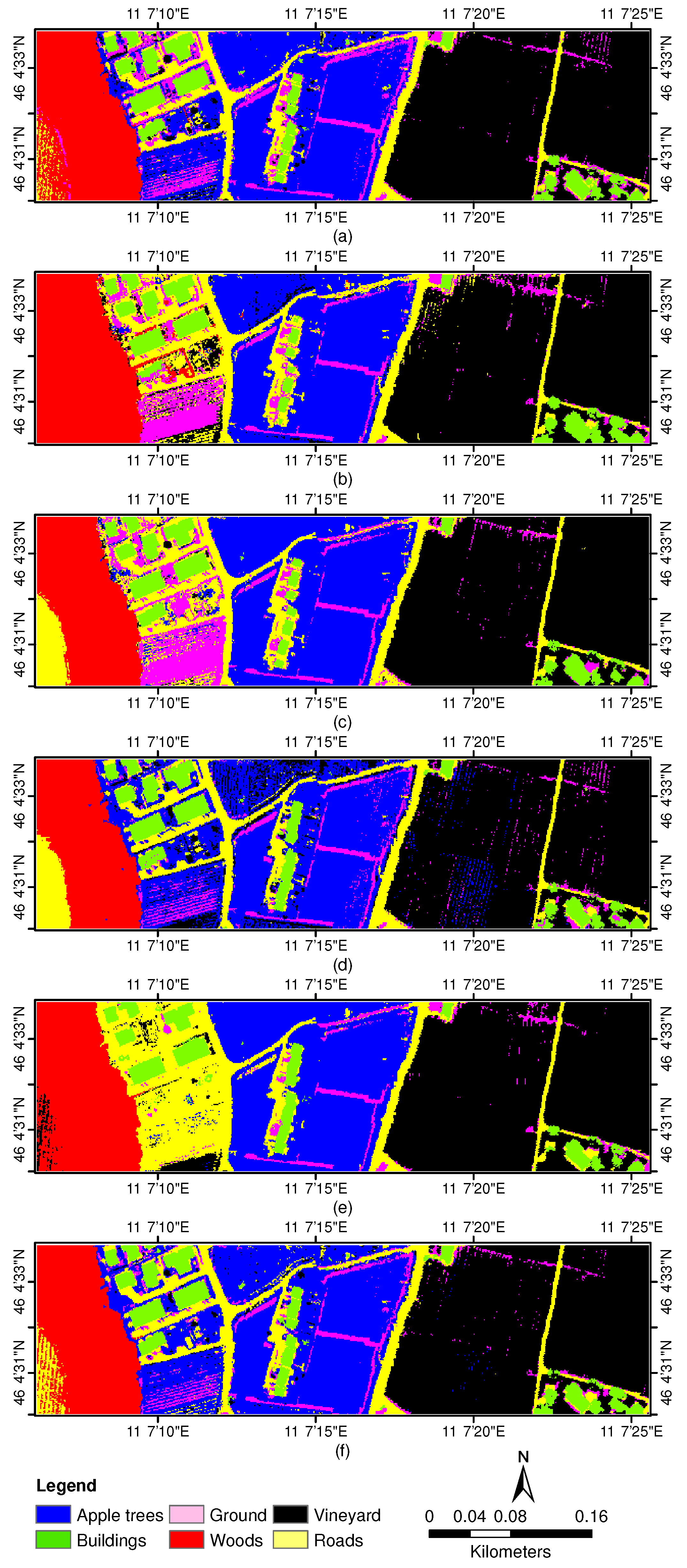
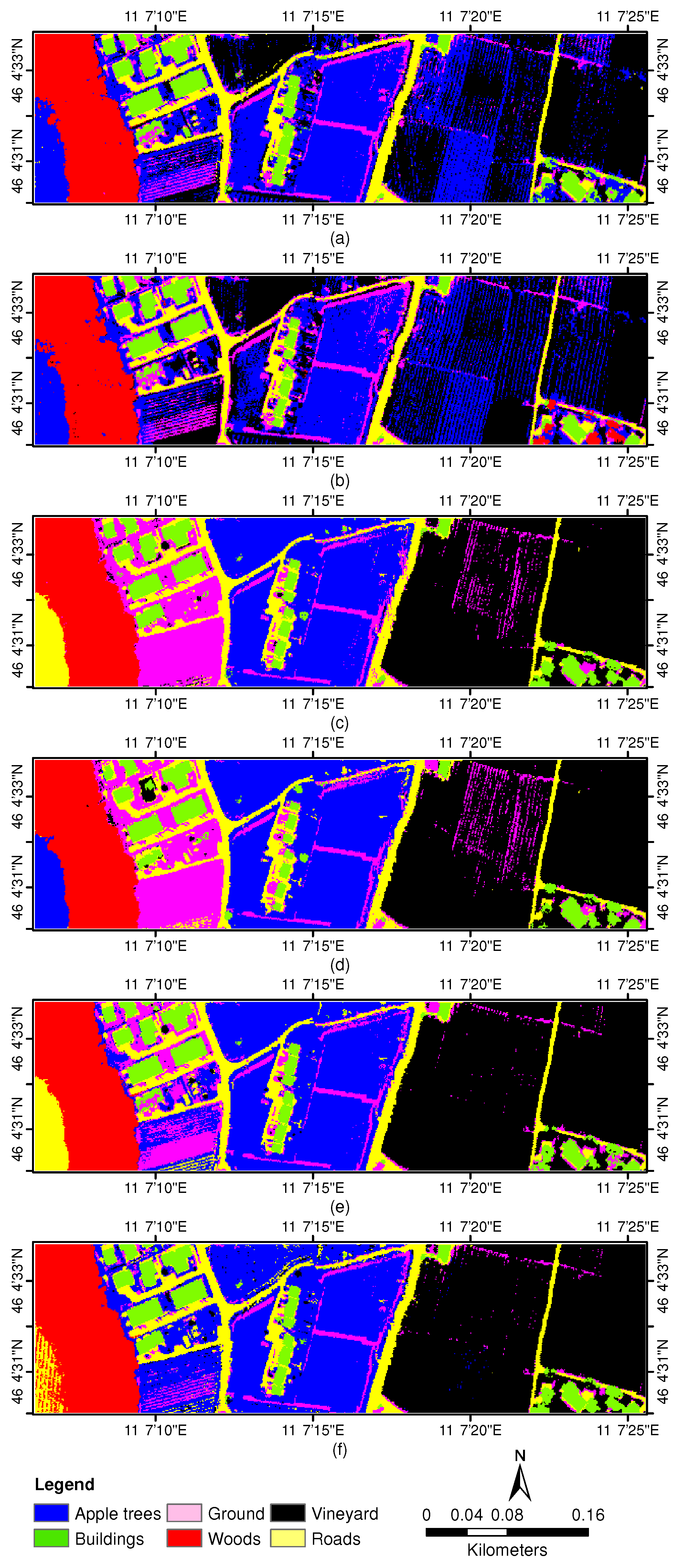
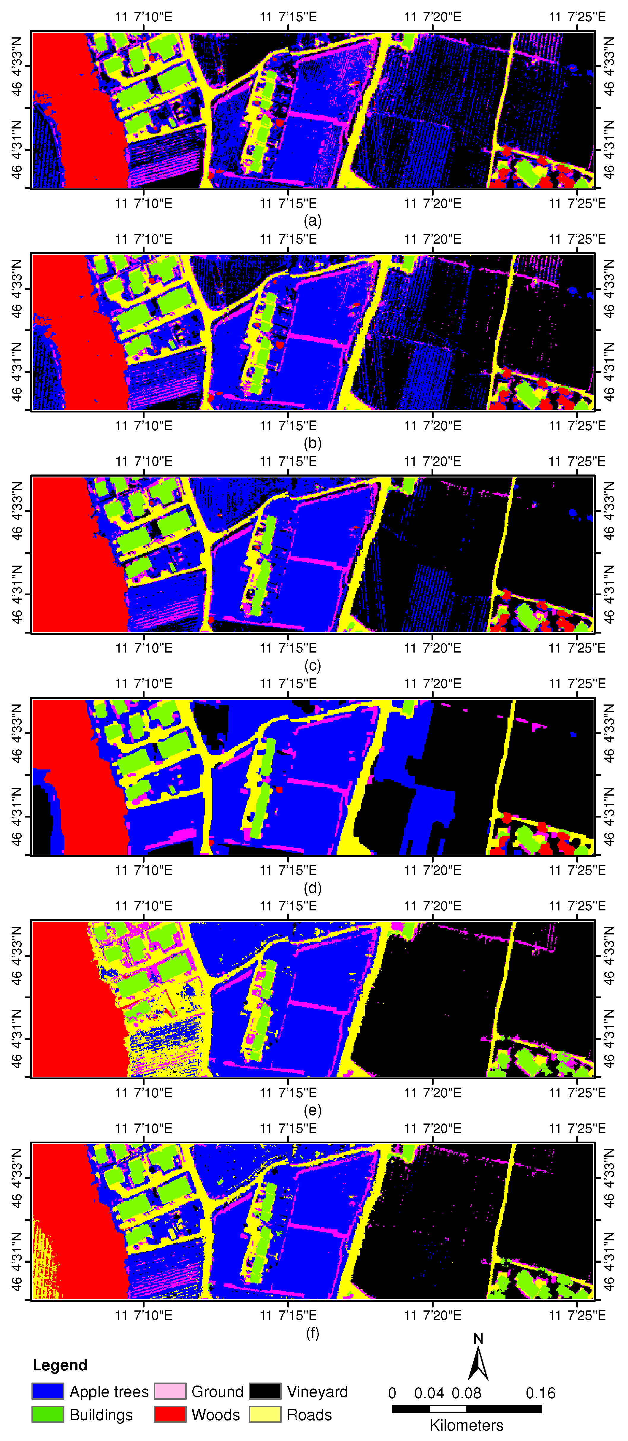
3.3. Experiments With Trento Data Sets

3.3.1. Experiment 1—Parameter Sensitiveness Analysis

As shown in Figure 8, the OAs increase as R also increase when $R\le 40$, then the OAs remains stable for different CHOTF-based methods. We experimentally set R = 100 in the following experiments. We also observe that ${\mathbf{X}}^H$⊗ EMAP(${\mathbf{X}}^H$) ⊗ AP(${\mathbf{X}}^L$) stably produces the highest accuracies in different cases. In the contrary, ${\mathbf{X}}^H$⊗ AP(${\mathbf{X}}^L$) produces the lowest and unstable accuracies, which is in accordance with the former experiment of Houston data sets.

3.3.2. Experiment 2—Comparison with DR-Based Methods

Table 6. Overall (OA), average (AA) and individual class accuracies (%), and kappa statistic ($\kappa$) obtained by SMLR based on DR-derived features and CHOTF-derived features for the Trento data sets.

Class	PCA	LGE	LPP	LDA	MFA	CHOTF
Apple trees	100.00	100.00	100.00	100.00	100.00	100.00
Buildings	98.00	93.39	97.31	98.79	82.78	98.62
Ground	96.45	94.36	93.53	95.82	73.70	95.62
Woods	99.95	99.99	99.97	99.70	99.97	99.91
Vineyard	99.80	99.80	99.63	98.40	99.70	99.75
Roads	89.48	94.27	92.66	91.34	96.22	91.15
Average accuracy	97.28	96.97	97.18	97.34	92.06	97.51
Overall accuracy	98.56	98.60	98.73	98.26	97.42	98.76
$\kappa$ statistic	0.981	0.981	0.983	0.977	0.965	0.983

reports the classification accuracies obtained by different dimensionality reduction methods. CHOTF outperforms the other DR-based methods with an OA of 98.76%, which is 0.03–1.3% higher than other methods. As for AA and $\kappa$ statistic, the improvements of CHOTF are 0.2–5% and 0–0.02%, respectively, compared to other DR-based methods. Figure 9 shows the classification maps, where significant differences can be found when classifying the class “Buildings” and “Roads”. It is interesting to note that LPP obtains a competitive classification performance with an OA of 98.73%. Another observation is that the classification results in region A (the large patch at the lower part and right next to the Woods) and region B (the lower-left corner) are quite different, which is due to the fact that the training samples are not available in these two regions [see Figure 2d]. Suspiciously, these two misclassified regions seem to have no effects on OAs. This is due to the fact that there are also no test samples in these two regions [see Figure 2c].

3.3.3. Experiment 3—Comparison with Independent Third-Order Tensor Factorization

Table 7. Overall (OA), average (AA) and individual class accuracies (%), and kappa statistic ($\kappa$) obtained by SMLR based on independent third-order tensor factorization based features for the Trento data sets.

Class	CPD	LL1	MLSVD	LMLRA	BTD	CHOTF
Apple trees	99.43	85.32	100.00	100.00	100.00	100.00
Buildings	95.83	93.63	97.97	89.29	94.94	98.62
Ground	96.45	97.49	95.82	95.62	95.82	95.62
Woods	99.19	98.41	99.90	99.84	99.93	99.91
Vineyard	91.07	77.28	96.21	94.61	99.78	99.75
Roads	89.22	87.52	88.15	90.04	89.48	91.15
Average accuracy	95.20	89.94	96.34	94.90	96.66	97.51
Overall accuracy	94.99	87.70	97.15	95.93	98.25	98.76
$\kappa$ statistic	0.934	0.839	0.962	0.946	0.977	0.983

reports the accuracies obtained by different third-order tensor factorization methods. CHOTF obtains the highest accuracies with significant performance improvements, e.g., around 0.5–4%, 1–8%, and 0.01–0.15 for OA, AA, and $\kappa$, respectively. Again, significant classification accuracies for the class “Buildings” and “Roads” can also be easily appreciated by visually inspecting the classification maps shown in Figure 10.

3.3.4. Experiment 4—Comparison with Different Classifiers Based on CHOTF-Derived Features

Table 8. Overall (OA), average (AA) and individual class accuracies (%), and kappa statistic ($\kappa$) obtained by different classifiers based on CHOTF-derived features for the Trento data sets.

Class	RF	SVM	MLRsub	LORSAL-MLL	MLR-GCK	SMLR
Apple trees	89.86	99.85	100.00	100.00	100.00	100.00
Buildings	97.28	97.52	98.83	98.28	97.73	98.62
Ground	95.20	96.24	94.99	96.24	95.20	95.62
Woods	99.32	99.18	99.65	99.87	99.98	99.91
Vineyard	85.02	95.67	98.00	100.00	99.96	99.75
Roads	91.34	89.51	88.59	92.75	91.75	91.15
Average accuracy	93.00	96.33	96.68	97.86	97.44	97.51
Overall accuracy	91.99	96.83	97.81	98.97	98.82	98.76
$\kappa$ statistic	0.894	0.958	0.971	0.986	0.984	0.983

reports the classification accuracies obtained by various classifiers based on the CHOTF-derived features. In this scene, LORSAL-MLL followed by MLR-GCK and SMLR reveals the best performance among other classifiers, which is not in accordance with the former experiments. This may due to the fact that the Trento scene contains may large homogeneous regions, which is beneficial for MRF-based spatial smoothing methods, i.e., the graph cuts method used in LORSAL-MLL. In addition, MLR-GCK obtained competitive results.

Figure 11 visually figures the classification maps, where the Vineyard and Apple trees regions illustrate significant differences between different maps. We observe that MLR-GCK and SMLR produce more accurate and smooth results in the Vineyard region. Even if LORSALL-MLL provides a higher OA and more smooth map, some regions are clearly misclassified, e.g., the Vineyard region.

4. Discussion

To have a more convincing validation, we compare the classification accuracies of the proposed method with some existing methods introduced in the literature recently. This comparison is fair since different methods were applied on the same and standard training and test samples.

4.1. For the University of Houston Data Sets

As reported in

Table 9. Overall (OA), average (AA), kappa statistic ($\kappa$), and elapsed time (s: seconds) obtained by different fusion methods for the University of Houston data sets.

Methods	Average Accuracy	Overall Accuracy	$\mathit{\kappa }$ Statistic	Elapsed Time
GGF [10]	83.03	80.48	0.788	34 s
EP+CNN [13]	90.39	89.71	0.888	∼700 s
Deep Fusion [7]	85.31	90.60	0.898
two-branch CNN [29]	90.11	87.98	0.870
three-stream CNN [15]	84.36	90.22	0.894
HyMCKs [16]	91.14	90.33	0.895	-
HODA [63]	88.79	87.05	0.860	18 s
LTDA [34]	88.83	87.12	0.860	60 s
CHOTF (ours)	91.93	91.24	0.905	254 s

, the proposed method outperforms the other methods. Compared to GGF [10], the accuracy increase in terms of OA is around 10%, which is not in accordance with the performance reported in [10]. This may due to the fact that we didn’t adopt the sampling and feature extraction methods used in GGF, whereas we only using the feature fusion scheme of GGF. Therefore, we apply GGF on our APs features as that of CHOTF, and we use a standard training and test samples to produce the accuracies via a SMLR classifier.

The OA increase is 1.4–4% compared to four deep learning based methods (i.e., EP+CNN [13], Deep Fusion [7], two-branch CNN [29], and three-stream CNN [15]). HyMCKs [16] provides competitive accuracies with an OA of 90.33%. In addition, when compared to tensor factorization based methods, the proposed method still outperforms HODA [63] and LTDA [34], with an increase of 4% in terms of OA. As for AA and $\kappa$ statistic, the improvements of performance are still significant.

As for the computational time, the proposed method costs 254s for one independent run. Whereas, the other two tensor-based methods are much faster, e.g., the elapsed time of HODA and LTDA are 18 s and 34 s, respectively. This is because HODA and LTDA adopt second-order tensors in tensor factorization. Deep learning based fusion methods are time consuming, e.g., two-branch CNN costs 735 s. In this context, the computational cost of the proposed method is reasonable considering the relatively higher accuracy.

4.2. For the Trento Data Sets

Table 10. Overall (OA), average (AA), kappa statistic ($\kappa$), and elapsed time (s: seconds) obtained by different fusion methods for the Trento data sets.

Methods	Average Accuracy	Overall Accuracy	$\mathit{\kappa }$ Statistic	Elapsed Time
GGF [10]	78.23	77.98	0.717	15 s
EP+CNN [13]	98.40	98.85	0.985	∼500 s
Deep Fusion [7]	77.17	97.83	0.971
two-branch CNN [29]	96.19	97.92	0.968
three-stream CNN [15]	79.47	97.91	0.973
HyMCKs [16]	98.18	98.97	0.986	-
HODA [63]	97.19	98.76	0.972	3 s
LTDA [34]	90.29	92.73	0.903	15 s
CHOTF (ours)	97.51	98.76	0.983	144 s

reports the classification accuracies of the proposed method as well as some existing methods introduced in the literature recently.

In this scene, we unfortunately found that HyMCKs obtained the highest OA among the other counterparts, with an OA of 98.97%. In addition, EP+CNN ranking second among all the considered methods, but CHOTF still outperforms Deep Fusion, two-branch CNN, and three-stream CNN. As for AA, EP+CNN obtained the best performance, with an AA of 98.40%. In terms of $\kappa$ statistic, HyMCKs again outperforms others, with the value of 0.986. However, when compared to the other two tensor factorization based methods, our method still produces better results. For example, the OA of CHOTF is 98.76%, which is the same as HODA but 6% higher than that of LTDA. CHOTF produces an AA of 97.51%, which is 0.4% and 7% higher than HODA and LTDA, respectively. In addition, the OA of CHOTF is only 0.21% lower than HyMCKs.

In this context, our method still provide good performance since it outperforms the other two related tensor-based methods and three deep learning based methods. In addition, CHOTF provides competitive results as HyMCKs in this experiment. Therefore, the above results also validate the superior performance of the proposed method. As for computational time, our method costs 144 s, and HODA only costs 3 s due to the relatively small scene in this experiment.

5. Conclusions

In this paper, we focus on the limitations of current flat-view matrix based methods by presenting a novel CHOTF framework for hyperspectral and LiDAR data classification based on morphological features. In particular, the framework generates third-order tensors based on spectral-spatial features, yields more latent features, and conducts classification by using SMLR. On the above analysis of the experimental results based on the real data sets, we can conclude that the proposed framework outperforms different DR-based methods, independent third-order tensor factorization based methods, and some recently proposed hyperspectral and LiDAR data classification methods. It should be noted that the proposed method is not restricted to LiDAR data but can also be applied to any other kind of 2.5D (i.e., image-like) data.

Although our experimental results are encouraging, further work on additional scenes and comparison methods should be conducted in future. In our work, we have introduced a CHOTF model for the first time in the literature of hyperspectral and LiDAR data classification. The involved spectral, spatial, and elevation information are jointly considered in the model, where some of the factors are shared among different data sources. However, the structures in tensors and the complementary information between tensors are not yet exploited. Our next work will focus on exploiting different structures and the complementary information in the model, which may be beneficial to overcome the missing values between different data sources.

References

1. Mura, M.D.; Prasad, S.; Pacifici, F.; Gamba, P.; Chanussot, J.; Benediktsson, J.A. Challenges and opportunities of multimodality and data fusion in remote sensing. Proc. IEEE 2015, 103, 1585–1601. [Google Scholar] [CrossRef]
2. Gomez-Chova, L.; Tuia, D.; Moser, G.; Camps-Valls, G. Multimodal classification of remote sensing images: A review and future directions. Proc. IEEE 2015, 103, 1560–1584. [Google Scholar] [CrossRef]
3. Debes, C.; Merentitis, A.; Heremans, R.; Hahn, J.; Frangiadakis, N.; van Kasteren, T.; Liao, W.Z.; Bellens, R.; Pizurica, A.; Gautama, S.; et al. Hyperspectral and LiDAR data fusion: Outcome of the 2013 GRSS data fusion contest. IEEE J. Sel. Top. Appl. Earth Obs. Remote Sens. 2014, 7, 2405–2418. [Google Scholar] [CrossRef]
4. Pedergnana, M.; Marpu, P.R.; Mura, M.D.; Benediktsson, J.A.; Bruzzone, L. Classification of remote sensing optical and LiDAR data using extended attribute profiles. IEEE J. Sel. Top. Signal Process. 2012, 6, 856–865. [Google Scholar] [CrossRef]
5. Khodadadzadeh, M.; Li, J.; Prasad, S.; Plaza, A. Fusion of hyperspectral and LiDAR remote sensing data using multiple feature learning. IEEE J. Sel. Top. Appl. Earth Obs. Remote Sens. 2015, 8, 2971–2983. [Google Scholar] [CrossRef]
6. Luo, R.B.; Liao, W.Z.; Zhang, H.Y.; Zhang, L.P.; Scheunders, P.; Pi, Y.G.; Philips, W. Fusion of hyperspectral and LiDAR data for classification of cloud-shadow mixed remote sensed scene. IEEE J. Sel. Top. Appl. Earth Obs. Remote Sens. 2017, 10, 3768–3781. [Google Scholar] [CrossRef]
7. Chen, Y.S.; Li, C.Y.; Ghamisi, P.; Jia, X.P.; Gu, Y.F. Deep fusion of remote sensing data for accurate classification. IEEE Geosci. Remote Sens. Lett. 2017, 14, 1253–1257. [Google Scholar] [CrossRef]
8. Wang, A.L.; He, X.; Ghamisi, P.; Chen, Y.S. LiDAR Data classification using morphological profiles and convolutional neural networks. IEEE Geosci. Remote Sens. Lett. 2018, 15, 774–778. [Google Scholar] [CrossRef]
9. Jahan, F.; Zhou, J.; Awrangjeb, M.; Gao, Y.S. Fusion of hyperspectral and LiDAR data using discriminant correlation analysis for land cover classification. IEEE J. Sel. Top. Appl. Earth Obs. Remote Sens. 2018, 11, 3905–3917. [Google Scholar] [CrossRef]
10. Liao, W.Z.; Pizurica, A.; Bellens, R.; Gautama, S.; Philips, W. Generalized graph-based fusion of hyperspectral and LiDAR data using morphological features. IEEE Geosci. Remote Sens. Lett. 2015, 12, 552–556. [Google Scholar] [CrossRef]
11. Gu, Y.F.; Wang, Q.W. Discriminative graph-based fusion of HSI and LiDAR data for urban area classification. IEEE Geosci. Remote Sens. Lett. 2017, 14, 906–910. [Google Scholar] [CrossRef]
12. Xia, J.S.; Yokoya, N.; Iwasaki, A. Fusion of hyperspectral and LiDAR data with a novel ensemble classifier. IEEE Geosci. Remote Sens. Lett. 2018, 15, 957–961. [Google Scholar] [CrossRef]
13. Ghamisi, P.; Hofle, B.; Zhu, X.X. Hyperspectral and LiDAR data fusion using extinction profiles and deep convolutional neural network. IEEE J. Sel. Top. Appl. Earth Obs. Remote Sens. 2017, 10, 3011–3024. [Google Scholar] [CrossRef]
14. Rasti, B.; Ghamisi, P.; Gloaguen, R. Hyperspectral and LiDAR fusion using extinction profiles and total variation component analysis. IEEE Trans. Geosci. Remote Sens. 2017, 55, 3997–4007. [Google Scholar] [CrossRef]
15. Li, H.; Ghamisi, P.; Soergel, U.; Zhu, X.X. Hyperspectral and LiDAR fusion using deep three-stream convolutional neural networks. Remote Sens. 2018, 10, 1649. [Google Scholar] [CrossRef]
16. Ghamisi, P.; Rash, B.; Benediktsson, J.A. Multisensor composite kernels based on extreme learning machines. IEEE Geosci. Remote Sens. Lett. 2019, 16, 196–200. [Google Scholar] [CrossRef]
17. Ni, L.; Gao, L.R.; Li, S.S.; Li, J.; Zhang, B. Edge-constrained Markov random field classification by integrating hyperspectral image with LiDAR data over urban areas. J. Appl. Remote Sens. 2014, 8, 085089. [Google Scholar] [CrossRef]
18. Yokoya, N.; Nakazawa, S.; Matsuki, T.; Iwasaki, A. Fusion of hyperspectral and LiDAR data for landscape visual quality assessment. IEEE J. Sel. Top. Appl. Earth Obs. Remote Sens. 2014, 7, 2419–2425. [Google Scholar] [CrossRef]
19. Zhang, Y.; Prasad, S. Multisource geospatial data fusion via local joint sparse representation. IEEE Trans. Geosci. Remote Sens. 2016, 54, 3265–3276. [Google Scholar] [CrossRef]
20. Rasti, B.; Ghamisi, P.; Plaza, J.; Plaza, A. Fusion of hyperspectral and LiDAR data using sparse and low-rank component analysis. IEEE Trans. Geosci. Remote Sens. 2017, 55, 6354–6365. [Google Scholar] [CrossRef]
21. Bigdeli, B.; Samadzadegan, F.; Reinartz, P. Feature grouping-based multiple fuzzy classifier system for fusion of hyperspectral and LiDAR data. J. Appl. Remote Sens. 2014, 8, 083509. [Google Scholar] [CrossRef]
22. Bigdeli, B.; Samadzadegan, F.; Reinartz, P. Fusion of hyperspectral and LiDAR data using decision template-based fuzzy multiple classifier system. Int. J. Appl. Earth Obse. Geoinf. 2015, 38, 309–320. [Google Scholar] [CrossRef]
23. Gu, Y.F.; Wang, Q.W.; Jia, X.P.; Benediktsson, J.A. A novel MKL model of integrating LiDAR data and MSI for urban area classification. IEEE Trans. Geosci. Remote Sens. 2015, 53, 5312–5326. [Google Scholar]
24. Zhang, Y.; Yang, H.L.; Prasad, S.; Pasolli, E.; Jung, J.; Crawford, M. Ensemble multiple kernel active learning for classification of multisource remote sensing data. IEEE J. Sel. Top. Appl. Earth Obs. Remote Sens. 2015, 8, 845–858. [Google Scholar] [CrossRef]
25. Zhang, Y.; Prasad, S. Locality preserving composite kernel feature extraction for multi-source geospatial image analysis. IEEE J. Sel. Top. Appl. Earth Obs. Remote Sens. 2015, 8, 1385–1392. [Google Scholar] [CrossRef]
26. Liu, X.L.; Bo, Y.C. Object-based crop species classification based on the combination of airborne hyperspectral images and LiDAR data. Remote Sens. 2015, 7, 922–950. [Google Scholar] [CrossRef]
27. Man, Q.; Dong, P.; Guo, H. Pixel- and feature-level fusion of hyperspectral and LiDAR data for urban land-use classification. Int. J. Remote Sens. 2015, 36, 1618–1644. [Google Scholar] [CrossRef]
28. Zhong, Z.S.; Fan, B.; Ding, K.; Li, H.C.; Xiang, S.M.; Pan, C.H. Efficient multiple feature fusion with hashing for hyperspectral imagery classification: A comparative study. IEEE Trans. Geosci. Remote Sens. 2016, 54, 4461–4478. [Google Scholar] [CrossRef]
29. Xu, X.D.; Li, W.; Ran, Q.; Du, Q.; Gao, L.R.; Zhang, B. Multisource remote sensing data classification based on convolutional neural network. IEEE Trans. Geosci. Remote Sens. 2018, 56, 937–949. [Google Scholar] [CrossRef]
30. Zhang, M.; Li, W.; Du, Q.; Gao, L.; Zhang, B. Feature extraction for classification of hyperspectral and LiDAR data using patch-to-patch CNN. IEEE Trans. Cybern. 2019, 1–12. [Google Scholar] [CrossRef] [PubMed]
31. Makantasis, K.; Doulamis, A.D.; Doulamis, N.D.; Nikitakis, A. Tensor-based classification models for hyperspectral data analysis. IEEE Trans. Geosci. Remote Sens. 2018, 56, 6884–6898. [Google Scholar] [CrossRef]
32. Vervliet, N.; Debals, O.; Sorber, L.; De Lathauwer, L. Breaking the curse of dimensionality using decompositions of incomplete tensors. IEEE Signal Process. Mag. 2014, 31, 71–79. [Google Scholar] [CrossRef]
33. Li, Q.; Schonfeld, D. Multilinear discriminant analysis for higher-order tensor data classification. IEEE Trans. Pattern Anal. Mach. Intell. 2014, 36, 2524–2537. [Google Scholar] [PubMed]
34. Zhong, Z.S.; Fan, B.; Duan, J.Y.; Wang, L.F.; Ding, K.; Xiang, S.M.; Pan, C.H. Discriminant tensor spectral-spatial feature extraction for hyperspectral image classification. IEEE Geosci. Remote Sens. Lett. 2015, 12, 1028–1032. [Google Scholar] [CrossRef]
35. He, Z.; Li, J.; Liu, L.; Liu, K.; Zhuo, L. Fast three-dimensional empirical mode decomposition of hyperspectral images for class-oriented multitask learning. IEEE Trans. Geosci. Remote Sens. 2016, 54, 6625–6643. [Google Scholar] [CrossRef]
36. Yang, L.X.; Wang, M.; Yang, S.Y.; Zhao, H.; Jiao, L.C.; Feng, X.C. Hybrid probabilistic sparse coding with spatial neighbor tensor for hyperspectral imagery classification. IEEE Trans. Geosci. Remote Sens. 2018, 56, 2491–2502. [Google Scholar] [CrossRef]
37. Fan, H.Y.; Li, C.; Guo, Y.L.; Kuang, G.Y.; Ma, J.Y. Spatial-spectral total variation regularized low-rank tensor decomposition for hyperspectral image denoising. IEEE Trans. Geosci. Remote Sens. 2018, 56, 6196–6213. [Google Scholar] [CrossRef]
38. An, J.L.; Zhang, X.R.; Zhou, H.Y.; Jiao, L.C. Tensor-based low-rank graph with multimanifold regularization for dimensionality reduction of hyperspectral images. IEEE Trans. Geosci. Remote Sens. 2018, 56, 4731–4746. [Google Scholar] [CrossRef]
39. Li, S.T.; Dian, R.W.; Fang, L.Y.; Bioucas-Dias, J.M. Fusing hyperspectral and multispectral images via coupled sparse tensor factorization. IEEE Trans. Image Process. 2018, 27, 4118–4130. [Google Scholar] [CrossRef]
40. Zhang, X.; Wen, G.J.; Dai, W. A tensor decomposition-based anomaly detection algorithm for hyperspectral image. IEEE Trans. Geosci. Remote Sens. 2016, 54, 5801–5820. [Google Scholar] [CrossRef]
41. Liu, Y.J.; Gao, G.M.; Gu, Y.F. Tensor matched subspace detector for hyperspectral target detection. IEEE Trans. Geosci. Remote Sens. 2017, 55, 1967–1974. [Google Scholar] [CrossRef]
42. Qian, Y.T.; Xiong, F.C.; Zeng, S.; Zhou, J.; Tang, Y.Y. Matrix-vector nonnegative tensor factorization for blind unmixing of hyperspectral imagery. IEEE Trans. Geosci. Remote Sens. 2017, 55, 1776–1792. [Google Scholar] [CrossRef]
43. Cichocki, A.; Mandic, D.P.; Phan, A.H.; Caiafa, C.F.; Zhou, G.X.; Zhao, Q.B.; De Lathauwer, L. Tensor decompositions for signal processing applications. IEEE Signal Process. Mag. 2015, 32, 145–163. [Google Scholar] [CrossRef]
44. Acar, E.; Papalexakis, E.E.; Gurdeniz, G.; Rasmussen, M.A.; Lawaetz, A.J.; Nilsson, M.; Bro, R. Structure-revealing data fusion. BMC Bioinform. 2014, 15, 239. [Google Scholar] [CrossRef]
45. Lahat, D.; Adali, T.; Jutten, C. Multimodal data fusion: An overview of methods, challenges, and prospects. Proc. IEEE 2015, 103, 1449–1477. [Google Scholar] [CrossRef]
46. Acar, E.; Rasmussen, M.A.; Savorani, F.; Næs, T.; Bro, R. Understanding data fusion within the framework of coupled matrix and tensor factorizations. Chemom. Intell. Lab. Syst. 2013, 129, 53–63. [Google Scholar] [CrossRef]
47. Sorber, L.; Van Barel, M.; De Lathauwer, L. Structured data fusion. IEEE J. Sel. Top. Signal Process. 2015, 9, 586–600. [Google Scholar] [CrossRef]
48. Pesaresi, M.; Benediktsson, J.A. A new approach for the morphological segmentation of high-resolution satellite imagery. IEEE Trans. Geosci. Remote Sens. 2001, 39, 309–320. [Google Scholar] [CrossRef] [Green Version]
49. Benediktsson, J.A.; Palmason, J.A.; Sveinsson, J.R. Classification of hyperspectral data from urban areas based on extended morphological profiles. IEEE Trans. Geosci. Remote Sens. 2005, 43, 480–491. [Google Scholar] [CrossRef]
50. Dalla Mura, M.; Benediktsson, J.A.; Waske, B.; Bruzzone, L. Morphological attribute profiles for the analysis of very high resolution images. IEEE Trans. Geosci. Remote Sens. 2010, 48, 3747–3762. [Google Scholar] [CrossRef]
51. Dalla Mura, M.; Benediktsson, J.A.; Waske, B.; Bruzzone, L. Extended profiles with morphological attribute filters for the analysis of hyperspectral data. Int. J. Remote Sens. 2010, 31, 5975–5991. [Google Scholar] [CrossRef]
52. Kolda, T.G.; Bader, B.W. Tensor decompositions and applications. SIAM Rev. 2009, 51, 455–500. [Google Scholar] [CrossRef]
53. Krishnapuram, B.; Carin, L.; Figueiredo, M.A.T.; Hartemink, A.J. Sparse multinomial logistic regression: Fast algorithms and generalization bounds. IEEE Trans. Pattern Anal. Mach. Intell. 2005, 27, 957–968. [Google Scholar] [CrossRef] [PubMed]
54. Li, J.; Bioucas-Dias, J.M.; Plaza, A. Hyperspectral image segmentation using a new Bayesian approach with active learning. IEEE Trans. Geosci. Remote Sens. 2011, 49, 3947–3960. [Google Scholar] [CrossRef]
55. Xue, Z.H.; Li, J.; Cheng, L.; Du, P.J. Spectral-spatial classification of hyperspectral data via morphological component analysis-based image separation. IEEE Trans. Geosci. Remote Sens. 2015, 53, 70–84. [Google Scholar]
56. Du, P.J.; Xue, Z.H.; Li, J.; Plaza, A. Learning discriminative sparse representations for hyperspectral image classification. IEEE J. Sel. Top. Signal Process. 2015, 9, 1089–1104. [Google Scholar] [CrossRef]
57. Xue, Z.H.; Du, P.J.; Li, J.; Su, H.J. Simultaneous sparse graph embedding for hyperspectral image classification. IEEE Trans. Geosci. Remote Sens. 2015, 53, 6114–6133. [Google Scholar] [CrossRef]
58. Xue, Z.H.; Du, P.J.; Li, J.; Su, H.J. Sparse graph regularization for hyperspectral remote sensing image classification. IEEE Trans. Geosci. Remote Sens. 2017, 55, 2351–2366. [Google Scholar] [CrossRef]
59. Xue, Z.H.; Du, P.J.; Li, J.; Su, H.J. Sparse graph regularization for robust crop mapping using hyperspectral remotely sensed imagery with very few in situ data. ISPRS J. Photogramm. Remote Sens. 2017, 124, 1–15. [Google Scholar] [CrossRef]
60. Zhou, S.G.; Xue, Z.H.; Du, P.J. Semisupervised stacked autoencoder with cotraining for hyperspectral image classification. IEEE Trans. Geosci. Remote Sens. 2019, 57, 1–14. [Google Scholar] [CrossRef]
61. Sorber, L.; Van Barel, M.; De Lathauwer, L. Optimization-based algorithms for tensor decompositions: Canonical polyadic decomposition, decomposition in rank-(Lr,Lr,1) terms, and a new generalization. SIAM J. Optim. 2013, 23, 695–720. [Google Scholar] [CrossRef]
62. De Lathauwer, L.; De Moor, B.; Vandewalle, J. A multilinear singular value decomposition. SIAM J. Matrix Anal. Appl. 2000, 21, 1253–1278. [Google Scholar] [CrossRef]
63. Phan, A.H.; Cichocki, A. Tensor decompositions for feature extraction and classification of high dimensional datasets. Nonlinear Theory Appl. IEICE 2010, 1, 37–68. [Google Scholar] [CrossRef] [Green Version]
64. Breiman, L. Random forests. Mach. Learn. 2001, 45, 5–32. [Google Scholar] [CrossRef]
65. Chang, C.C.; Lin, C.J. LIBSVM: A library for support vector machines. ACM Trans. Intell. Syst. Technol. 2011, 2, 27. [Google Scholar] [CrossRef]
66. Li, J.; Bioucas-Dias, J.M.; Plaza, A. Spectral-spatial hyperspectral image segmentation using subspace multinomial logistic regression and Markov random fields. IEEE Trans. Geosci. Remote Sens. 2012, 50, 809–823. [Google Scholar] [CrossRef]
67. Li, J.; Marpu, P.R.; Plaza, A.; Bioucas-Dias, J.M.; Benediktsson, J.A. Generalized composite kernel framework for hyperspectral image classification. IEEE Trans. Geosci. Remote Sens. 2013, 51, 4816–4829. [Google Scholar] [CrossRef]
Figure 1. University of Houston data sets. (a) False color composite image (R: 59, G: 40, B: 23). (b) LiDAR-derived DSM. (c) Test set. (d) Training set.
Remotesensing 11 01959 g001
Figure 2. Trento data sets. (a) False color composite image (R: 40, G: 20, B: 10). (b) LiDAR-derived DSM. (c) Test set. (d) Training set.
Remotesensing 11 01959 g002
Figure 3. Flowchart of the proposed framework for hyperspectral and LiDAR data classification.
Remotesensing 11 01959 g003
Figure 4. Overall accuracies as a function of the number of rank-one terms (R) for the University of Houston Data Sets. R is experimentally set to 100.
Remotesensing 11 01959 g004
Figure 5. Classification maps obtained by SMLR based on DR-derived features and CHOTF-derived features for the University of Houston data sets. (a) PCA (OA = 88.37%), (b) LGE (OA = 88.51%), (c) LPP (OA = 85.59%), (d) LDA (OA = 88.32%), (e) MFA (OA = 86.96%), (f) CHOTF (OA = 91.24%).
Remotesensing 11 01959 g005
Figure 6. Classification maps obtained by SMLR based on independent third-order factorization based features for the University of Houston data sets. (a) CPD (OA = 85.36%), (b) LL1 (OA = 70.86%), (c) MLSVD (OA = 87.94%), (d) LMLRA (OA = 86.21%), (e) BTD (OA = 87.50%), (f) CHOTF (OA = 91.24%).
Remotesensing 11 01959 g006
Figure 7. Classification maps obtained by different classifiers based on CHOTF-derived features for the University of Houston data sets. (a) RF (OA = 78.51%), (b) SVM (OA = 82.92%), (c) MLRsub (OA = 89.50%), (d) LORSALL-MLL (OA = 90.25%), (e) MLR-GCK (OA = 89.33%), (f) SMLR (OA = 91.24%).
Remotesensing 11 01959 g007
Figure 8. Overall accuracies as a function of the number of rank-one terms (R) for the Trento data sets. R is experimentally set to 100.
Remotesensing 11 01959 g008
Figure 9. Classification maps obtained by SMLR based on DR-derived features and CHOTF-derived features for the Trento data sets. (a) PCA (OA = 98.56%), (b) LGE (OA = 98.60%), (c) LPP (OA = 98.73%), (d) LDA (OA = 98.26%), (e) MFA (OA = 97.42%), (f) CHOTF (OA = 98.76%).
Remotesensing 11 01959 g009
Figure 10. Classification maps obtained by SMLR based on independent third-order tensor factorization based features for the Trento data sets. (a) CPD (OA = 94.99%), (b) LL1 (OA = 87.70%), (c) MLSVD (OA = 97.15%), (d) LMLRA (OA = 95.93%), (e) BTD (OA = 98.25%), (f) CHOTF (OA = 98.76%).
Remotesensing 11 01959 g010
Figure 11. Classification maps obtained by different classifiers based on CHOTF-derived features for the Trento data sets. (a) RF (OA = 91.99%), (b) SVM (OA = 96.83%), (c) MLRsub (OA = 97.81%), (d) LORSAL-MLL (OA = 98.97%), (e) MLR-GCK (OA = 98.82%), (f) SMLR (OA = 98.76%).
Remotesensing 11 01959 g011