Evaluation of the Uncertainty in Satellite-Based Crop State Variable Retrievals Due to Site and Growth Stage Specific Factors and Their Potential in Coupling with Crop Growth Models

 , ,
, , 
Abstract
1. Introduction
1.1. Background
1.2. Overview
2. Materials and Methods
2.1. Data
2.2. Hybrid-Maize (HM) Simulations
2.3. Methods
2.3.1. Evaluation of HM Simulations
2.3.2. Regression-Based LAI and LUECanopy Retrieval
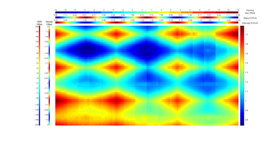
2.3.3. Satellite Retrieval and Crop Growth Model Sensitivity Analysis
2.3.4. Evaluation of Uncertainty of LAI and LUECanopy Retrievals Due to Site and Growth Stage Specific Factors with Temporal Analysis
- Using the LAIGROUND dataset with LANDSAT imagery better allows for the use of exact point measurements in fields and is thus less likely to be subject to uncertainty in training due to the inhomogeneity of LAI in the field, which can be significant [95].
2.3.5. Training LAI and LUECanopy Retrievals with HM Simulations
3. Results
3.1. Evaluation of HM Simulations
3.2. Regression-Based LAI and LUECanopy Retrieval
3.3. Satellite Retrieval and Crop Growth Model Sensitivity Analysis
3.4. Evaluation of Uncertainty of LAI and LUECanopy Retrievals Due to Site and Growth Stage Specific Factors with Temporal Analysis
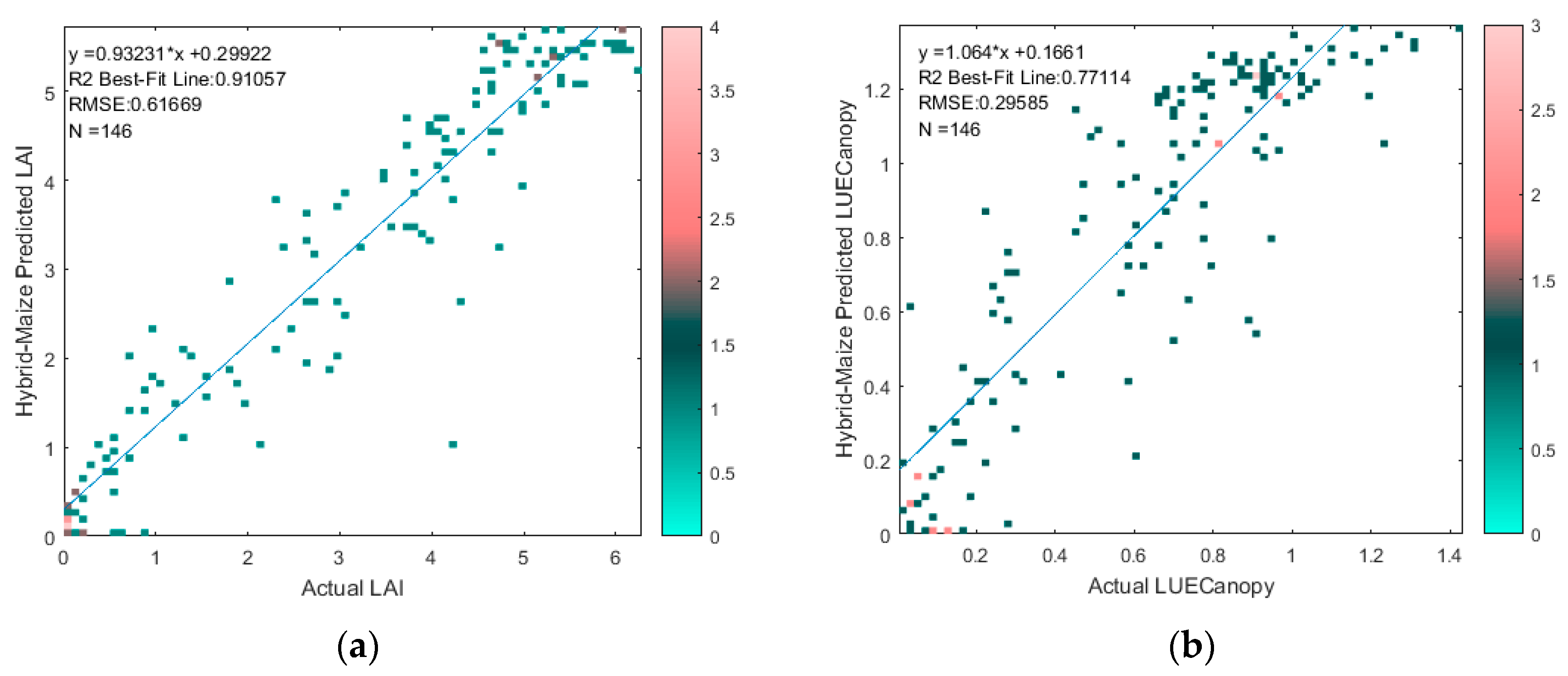
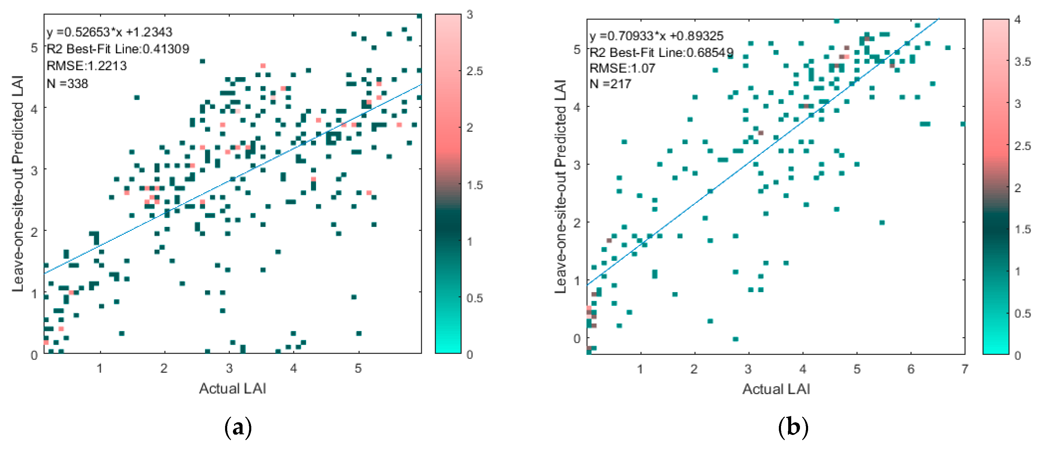
3.5. Training LAI and LUECanopy Retrievals with HM Simulations
4. Discussion
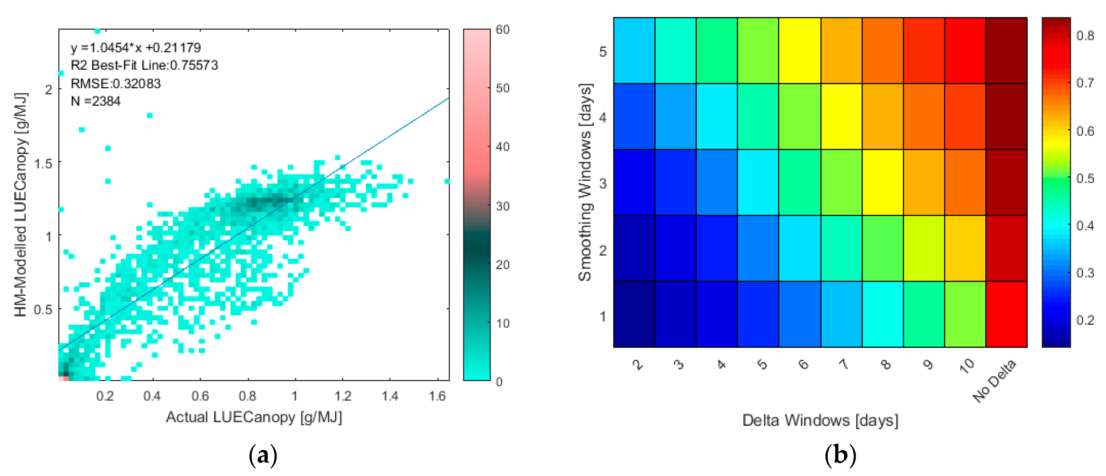
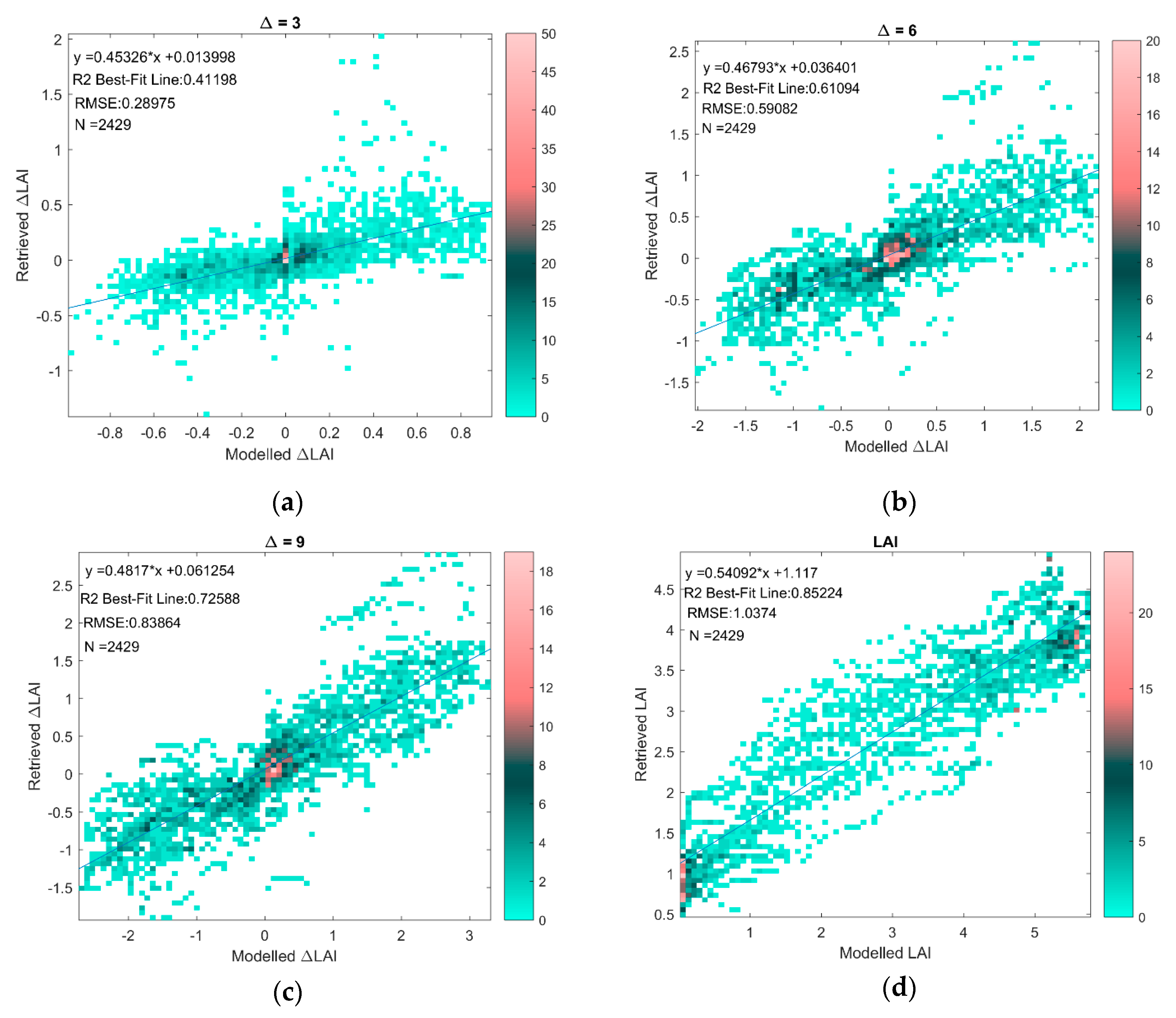
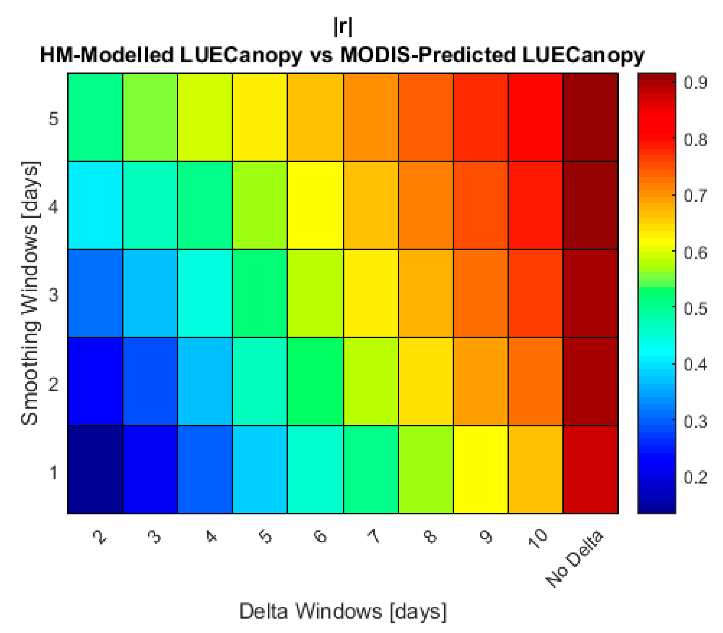
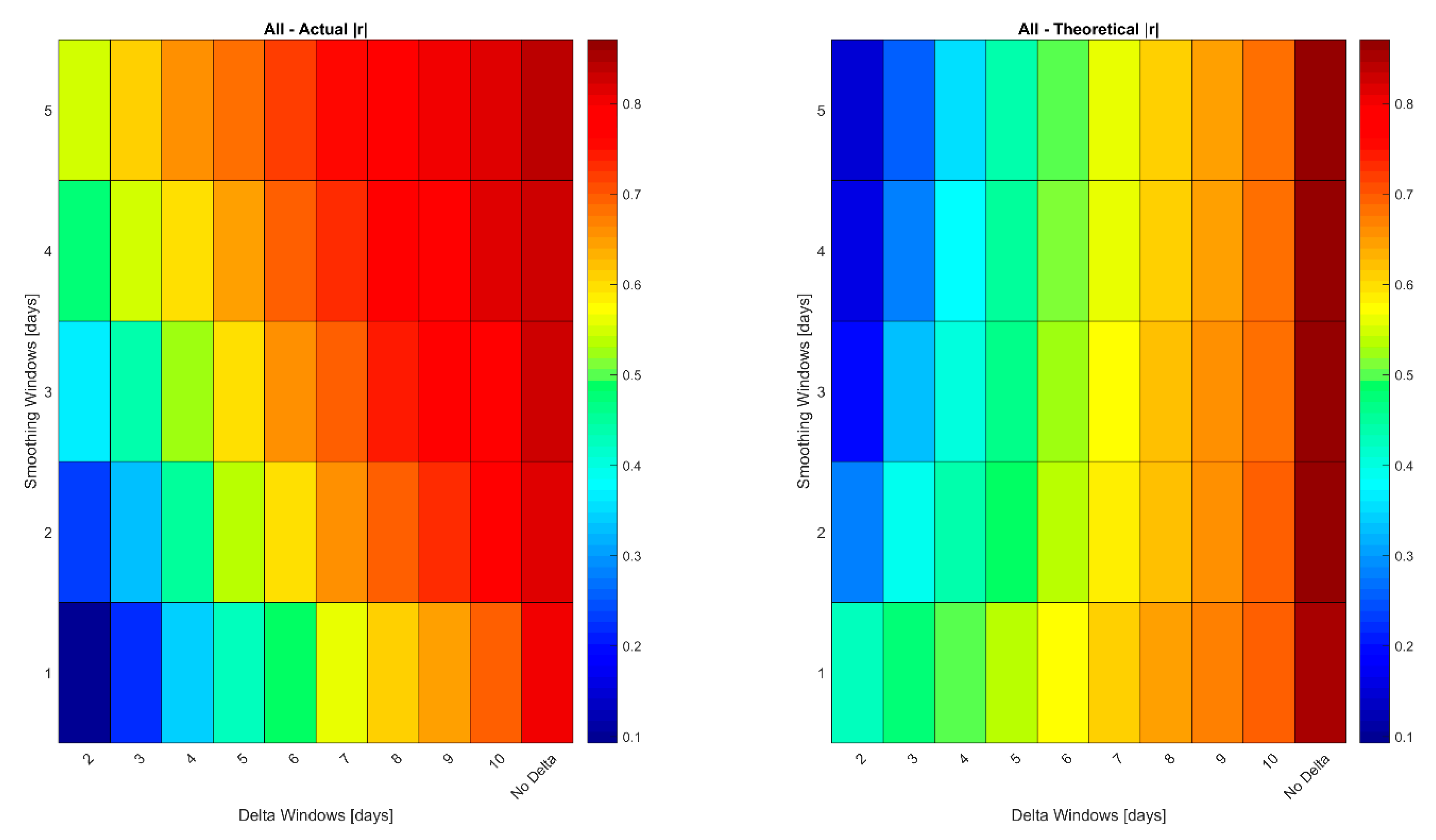
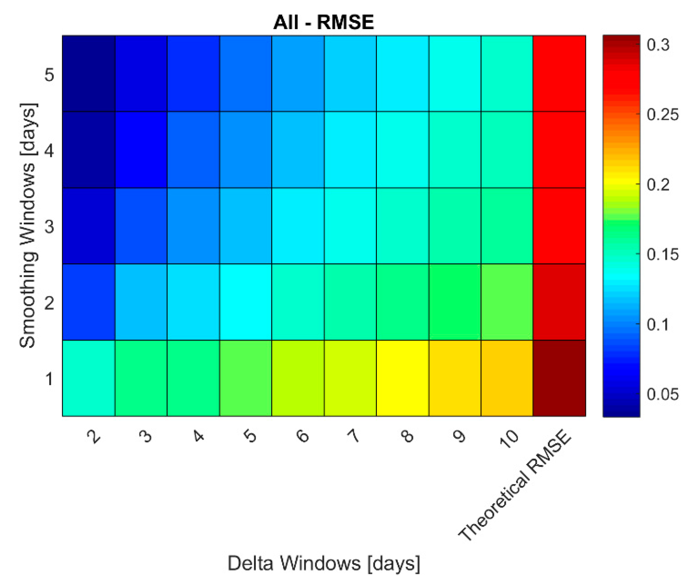
- As Δ increases, the correlation between the error in the retrieved LAI or LUECanopy at t2 relative to t1 decreases because the measurements are more likely to be in different growth stages.
- As Δ increases, the magnitude of the retrieved ΔLAI or ΔLUECanopy increases relative to the remaining error which is not cancelled when calculating the change in the retrieved variables from the variables themselves, i.e., e[t2] − e[t1].
5. Conclusions
Supplementary Materials
Author Contributions
Funding
Acknowledgments
Conflicts of Interest
References
- Teixeira, E.I.; Zhao, G.; de Ruiter, J.; Brown, H.; Ausseil, A.-G.; Meenken, E.; Ewert, F. The interactions between genotype, management and environment in regional crop modeling. Eur. J. Agron. 2017, 88, 106–115. [Google Scholar] [CrossRef]
- Archontoulis, S.V.; Miguez, F.E.; Moore, K.J. Evaluating APSIM maize, soil water, soil nitrogen, manure, and soil temperature modules in the Midwestern United States. Agron. J. 2014, 106, 1025–1040. [Google Scholar] [CrossRef]
- Keating, B.; Carberry, P.; Hammer, G.; Probert, M.; Robertson, M.; Holzworth, D.; Huth, N.; Hargreaves, J.N.; Meinke, H.; Hochman, Z.; et al. An overview of APSIM, a model designed for farming systems simulation. Eur. J. Agron. 2003, 18, 267–288. [Google Scholar] [CrossRef]
- Donatelli, M.; Magarey, R.D.; Bregaglio, S.; Willocquet, L.; Whish, J.P.M.; Savary, S. Modeling the impacts of pests and diseases on agricultural systems. Agric. Syst. 2017, 155, 213–224. [Google Scholar] [CrossRef]
- Grassini, P.; Thorburn, J.; Burr, C.; Cassman, K.G. High-yield irrigated maize in the Western, U.S. Corn Belt: I. On-farm yield, yield potential, and impact of agronomic practices. Field Crops Res. 2011, 120, 142–150. [Google Scholar] [CrossRef]
- Morell, F.J.; Yang, H.S.; Cassman, K.G.; Wart, J.V.; Elmore, R.W.; Licht, M.; Coulter, J.A.; Ciampitti, I.A.; Pittelkow, C.M.; Brouder, S.M.; et al. Can crop simulation models be used to predict local to regional maize yields and total production in the U.S. Corn Belt? Field Crops Res. 2016, 192, 1–12. [Google Scholar] [CrossRef]
- Carberry, P.S.; Hochman, Z.; Hunt, J.R.; Dalgliesh, N.P.; McCown, R.L.; Whish, J.P.M.; Robertson, M.J.; Foale, M.A.; Poulton, P.L.; van Rees, H. Re-inventing model-based decision support with Australian dryland farmers. 3. Relevance of APSIM to commercial crops. Crop Pasture Sci. 2009, 60, 1044–1056. [Google Scholar] [CrossRef]
- Jin, X.; Kumar, L.; Li, Z.; Feng, H.; Xu, X.; Yang, G.; Wang, J. A review of data assimilation of remote sensing and crop models. Eur. J. Agron. 2018, 92, 141–152. [Google Scholar] [CrossRef]
- Dorigo, W.A.; Zurita-Milla, R.; de Wit, A.J.W.; Brazile, J.; Singh, R.; Schaepman, M.E. A review on reflective remote sensing and data assimilation techniques for enhanced agroecosystem modeling. Int. J. Appl. Earth Obs. Geoinf. 2007, 9, 165–193. [Google Scholar] [CrossRef]
- Guérif, M.; Duke, C. Adjustment procedures of a crop model to the site specific characteristics of soil and crop using remote sensing data assimilation. Agric. Ecosyst. Environ. 2000, 81, 57–69. [Google Scholar] [CrossRef]
- Constantin, J.; Raynal, H.; Casellas, E.; Hoffmann, H.; Bindi, M.; Doro, L.; Eckersten, H.; Gaiser, T.; Grosz, B.; Haas, E.; et al. Management and spatial resolution effects on yield and water balance at regional scale in crop models. Agric. For. Meteorol. 2019, 275, 184–195. [Google Scholar] [CrossRef]
- He, J.; Jones, J.W.; Graham, W.D.; Dukes, M.D. Influence of likelihood function choice for estimating crop model parameters using the generalized likelihood uncertainty estimation method. Agric. Syst. 2010, 103, 256–264. [Google Scholar] [CrossRef]
- He, D.; Wang, E.; Wang, J.; Robertson, M.J. Data requirement for effective calibration of process-based crop models. Agric. For. Meteorol. 2017, 234–235, 136–148. [Google Scholar] [CrossRef]
- Confalonieri, R.; Bregaglio, S.; Acutis, M. Quantifying uncertainty in crop model predictions due to the uncertainty in the observations used for calibration. Ecol. Model. 2016, 328, 72–77. [Google Scholar] [CrossRef]
- Kang, Y.; Özdoğan, M. Field-level crop yield mapping with Landsat using a hierarchical data assimilation approach. Remote Sens. Environ. 2019, 228, 144–163. [Google Scholar] [CrossRef]
- Battude, M.; Al Bitar, A.; Morin, D.; Cros, J.; Huc, M.; Marais Sicre, C.; Le Dantec, V.; Demarez, V. Estimating maize biomass and yield over large areas using high spatial and temporal resolution Sentinel-2 like remote sensing data. Remote Sens. Environ. 2016, 184, 668–681. [Google Scholar] [CrossRef]
- Ines, A.V.M.; Das, N.N.; Hansen, J.W.; Njoku, E.G. Assimilation of remotely sensed soil moisture and vegetation with a crop simulation model for maize yield prediction. Remote Sens. Environ. 2013, 138, 149–164. [Google Scholar] [CrossRef]
- Jégo, G.; Pattey, E.; Liu, J. Using Leaf Area Index, retrieved from optical imagery, in the STICS crop model for predicting yield and biomass of field crops. Field Crops Res. 2012, 131, 63–74. [Google Scholar] [CrossRef]
- Battisti, R.; Sentelhas, P.C.; Boote, K.J. Inter-comparison of performance of soybean crop simulation models and their ensemble in southern Brazil. Field Crops Res. 2017, 200, 28–37. [Google Scholar] [CrossRef]
- Angulo, C.; Rötter, R.; Lock, R.; Enders, A.; Fronzek, S.; Ewert, F. Implication of crop model calibration strategies for assessing regional impacts of climate change in Europe. Agric. For. Meteorol. 2013, 170, 32–46. [Google Scholar] [CrossRef]
- Rosenzweig, C.; Elliott, J.; Deryng, D.; Ruane, A.C.; Müller, C.; Arneth, A.; Boote, K.J.; Folberth, C.; Glotter, M.; Khabarov, N.; et al. Assessing agricultural risks of climate change in the 21st century in a global gridded crop model intercomparison. Proc. Natl. Acad. Sci. USA 2014, 111, 3268–3273. [Google Scholar] [CrossRef]
- Lecerf, R.; Ceglar, A.; López-Lozano, R.; Van Der Velde, M.; Baruth, B. Assessing the information in crop model and meteorological indicators to forecast crop yield over Europe. Agric. Syst. 2019, 168, 191–202. [Google Scholar] [CrossRef]
- Woodard, J.D. Integrating high resolution soil data into federal crop insurance policy: Implications for policy and conservation. Environ. Sci. Policy 2016, 66, 93–100. [Google Scholar] [CrossRef]
- Grassini, P.; Wolf, J.; Tittonell, P.; Hochman, Z. Yield gap analysis with local to global relevance—A review. Field Crop. Res. 2013, 143, 4–17. [Google Scholar] [CrossRef]
- Ramirez-Villegas, J.; Koehler, A.-K.; Challinor, A.J. Assessing uncertainty and complexity in regional-scale crop model simulations. Eur. J. Agron. 2017, 88, 84–95. [Google Scholar] [CrossRef]
- Reynolds, M.; Kropff, M.; Crossa, J.; Koo, J.; Kruseman, G.; Molero, A.M.; Rutkoski, J.; Schulthess, U.; Balwinder-Singh; Sonder, K.; et al. Role of Modeling in International Crop Research: Overview and Some Case Studies. Agronomy 2018, 8, 291. [Google Scholar] [CrossRef]
- Kang, Y.; Özdoğan, M.; Zipper, S.; Román, M.; Walker, J.; Hong, S.; Marshall, M.; Magliulo, V.; Moreno, J.; Alonso, L.; et al. How Universal Is the Relationship between Remotely Sensed Vegetation Indices and Crop Leaf Area Index? A Global Assessment. Remote Sens. 2016, 8, 597. [Google Scholar] [CrossRef]
- Corti, M.; Cavalli, D.; Cabassi, G.; Marino Gallina, P.; Bechini, L. Does remote and proximal optical sensing successfully estimate maize variables? A review. Eur. J. Agron. 2018, 99, 37–50. [Google Scholar] [CrossRef]
- Wang, Y.; Zhang, K.; Tang, C.; Cao, Q.; Tian, Y.; Zhu, Y.; Cao, W.; Liu, X.; Wang, Y.; Zhang, K.; et al. Estimation of Rice Growth Parameters Based on Linear Mixed-Effect Model Using Multispectral Images from Fixed-Wing Unmanned Aerial Vehicles. Remote Sens. 2019, 11, 1371. [Google Scholar] [CrossRef]
- Clevers, J.; Kooistra, L.; van den Brande, M.; Clevers, J.G.P.W.; Kooistra, L.; Van den Brande, M.M.M. Using Sentinel-2 Data for Retrieving LAI and Leaf and Canopy Chlorophyll Content of a Potato Crop. Remote Sens. 2017, 9, 405. [Google Scholar] [CrossRef]
- Gonsamo, A.; Chen, J.M. Improved LAI Algorithm Implementation to MODIS Data by Incorporating Background, Topography, and Foliage Clumping Information. IEEE Trans. Geosci. Remote Sens. 2014, 52, 1076–1088. [Google Scholar] [CrossRef]
- Liu, J.; Pattey, E.; Jégo, G. Assessment of vegetation indices for regional crop green LAI estimation from Landsat images over multiple growing seasons. Remote Sens. Environ. 2012, 123, 347–358. [Google Scholar] [CrossRef]
- Li, Z.; Jin, X.; Yang, G.; Drummond, J.; Yang, H.; Clark, B.; Li, Z.; Zhao, C.; Li, Z.; Jin, X.; et al. Remote Sensing of Leaf and Canopy Nitrogen Status in Winter Wheat (Triticum aestivum L.) Based on N-PROSAIL Model. Remote Sens. 2018, 10, 1463. [Google Scholar] [CrossRef]
- Boren, E.J.; Boschetti, L.; Johnson, D.M.; Boren, E.J.; Boschetti, L.; Johnson, D.M. Characterizing the Variability of the Structure Parameter in the PROSPECT Leaf Optical Properties Model. Remote Sens. 2019, 11, 1236. [Google Scholar] [CrossRef]
- Gitelson, A.A.; Peng, Y.; Arkebauer, T.J.; Schepers, J. Relationships between gross primary production, green LAI, and canopy chlorophyll content in maize: Implications for remote sensing of primary production. Remote Sens. Environ. 2014, 144, 65–72. [Google Scholar] [CrossRef]
- Pinter, P.J.; Jackson, R.D.; Ezra, C.E.; Gausman, H.W. Sun-angle and canopy-architecture effects on the spectral reflectance of six wheat cultivars. Int. J. Remote Sens. 1985, 6, 1813–1825. [Google Scholar] [CrossRef]
- Jacquemoud, S.; Verhoef, W.; Baret, F.; Bacour, C.; Zarco-Tejada, P.J.; Asner, G.P.; François, C. PROSPECT + SAIL models: A review of use for vegetation characterization. Remote Sens. Environ. 2009, 113, S56–S66. [Google Scholar] [CrossRef]
- Combal, B.; Baret, F.; Weiss, M.; Trubuil, A.; Macé, D.; Pragnère, A.; Myneni, R.; Knyazikhin, Y.; Wang, L. Retrieval of canopy biophysical variables from bidirectional reflectance: Using prior information to solve the ill-posed inverse problem. Remote Sens. Environ. 2003, 84, 1–15. [Google Scholar] [CrossRef]
- Houborg, R.; McCabe, M.F. Adapting a regularized canopy reflectance model (REGFLEC) for the retrieval challenges of dryland agricultural systems. Remote Sens. Environ. 2016, 186, 105–120. [Google Scholar] [CrossRef]
- Houborg, R.; McCabe, M.; Cescatti, A.; Gao, F.; Schull, M.; Gitelson, A. Joint leaf chlorophyll content and leaf area index retrieval from Landsat data using a regularized model inversion system (REGFLEC). Remote Sens. Environ. 2015, 159, 203–221. [Google Scholar] [CrossRef]
- Xiao, Z.; Liang, S.; Wang, J.; Song, J.; Wu, X. A Temporally Integrated Inversion Method for Estimating Leaf Area Index From MODIS Data. IEEE Trans. Geosci. Remote Sens. 2009, 47, 2536–2545. [Google Scholar] [CrossRef]
- Koetz, B.; Baret, F.; Poilvé, H.; Hill, J. Use of coupled canopy structure dynamic and radiative transfer models to estimate biophysical canopy characteristics. Remote Sens. Environ. 2005, 95, 115–124. [Google Scholar] [CrossRef]
- Atzberger, C. Object-based retrieval of biophysical canopy variables using artificial neural nets and radiative transfer models. Remote Sens. Environ. 2004, 93, 53–67. [Google Scholar] [CrossRef]
- Dorigo, W.; Richter, R.; Baret, F.; Bamler, R.; Wagner, W.; Dorigo, W.; Richter, R.; Baret, F.; Bamler, R.; Wagner, W. Enhanced automated canopy characterization from hyperspectral data by a novel two step radiative transfer model inversion approach. Remote Sens. 2009, 1, 1139–1170. [Google Scholar] [CrossRef]
- Jin, X.; Li, Z.; Feng, H.; Xu, X.; Yang, G. Newly Combined Spectral Indices to Improve Estimation of Total Leaf Chlorophyll Content in Cotton. IEEE J. Sel. Top. Appl. Earth Obs. Remote Sens. 2014, 7, 4589–4600. [Google Scholar] [CrossRef]
- Xiao, Y.; Zhao, W.; Zhou, D.; Gong, H. Sensitivity Analysis of Vegetation Reflectance to Biochemical and Biophysical Variables at Leaf, Canopy, and Regional Scales. IEEE Trans. Geosci. Remote Sens. 2014, 52, 4014–4024. [Google Scholar] [CrossRef]
- Verrelst, J.; Camps-Valls, G.; Muñoz-Marí, J.; Rivera, J.P.; Veroustraete, F.; Clevers, J.G.P.W.; Moreno, J. Optical remote sensing and the retrieval of terrestrial vegetation bio-geophysical properties—A review. ISPRS J. Photogramm. Remote Sens. 2015, 108, 273–290. [Google Scholar] [CrossRef]
- Darvishzadeh, R.; Atzberger, C.; Skidmore, A.; Schlerf, M. Mapping grassland leaf area index with airborne hyperspectral imagery: A comparison study of statistical approaches and inversion of radiative transfer models. ISPRS J. Photogramm. Remote Sens. 2011, 66, 894–906. [Google Scholar] [CrossRef]
- Atzberger, C.; Guérif, M.; Baret, F.; Werner, W. Comparative analysis of three chemometric techniques for the spectroradiometric assessment of canopy chlorophyll content in winter wheat. Comput. Electron. Agric. 2010, 73, 165–173. [Google Scholar] [CrossRef]
- Kiala, Z.; Odindi, J.; Mutanga, O.; Peerbhay, K. Comparison of partial least squares and support vector regressions for predicting leaf area index on a tropical grassland using hyperspectral data. J. Appl. Remote Sens. 2016, 10, 036015. [Google Scholar] [CrossRef]
- Wang, L.; Chang, Q.; Li, F.; Yan, L.; Huang, Y.; Wang, Q.; Luo, L.; Wang, L.; Chang, Q.; Li, F.; et al. Effects of growth stage development on paddy rice leaf area index prediction models. Remote Sens. 2019, 11, 361. [Google Scholar] [CrossRef]
- Machwitz, M.; Giustarini, L.; Bossung, C.; Frantz, D.; Schlerf, M.; Lilienthal, H.; Wandera, L.; Matgen, P.; Hoffmann, L.; Udelhoven, T. Enhanced biomass prediction by assimilating satellite data into a crop growth model. Environ. Model. Softw. 2014, 62, 437–453. [Google Scholar] [CrossRef]
- Weiss, M.; Troufleau, D.; Baret, F.; Chauki, H.; Prévot, L.; Olioso, A.; Bruguier, N.; Brisson, N. Coupling canopy functioning and radiative transfer models for remote sensing data assimilation. Agric. For. Meteorol. 2001, 108, 113–128. [Google Scholar] [CrossRef]
- Zhang, L.; Guo, C.L.; Zhao, L.Y.; Zhu, Y.; Cao, W.X.; Tian, Y.C.; Cheng, T.; Wang, X. Estimating wheat yield by integrating the WheatGrow and PROSAIL models. Field Crops Res. 2016, 192, 55–66. [Google Scholar] [CrossRef]
- Thorp, K.R.; Wang, G.; West, A.L.; Moran, M.S.; Bronson, K.F.; White, J.W.; Mon, J. Estimating crop biophysical properties from remote sensing data by inverting linked radiative transfer and ecophysiological models. Remote Sens. Environ. 2012, 124, 224–233. [Google Scholar] [CrossRef]
- Jin, Z.; Prasad, R.; Shriver, J.; Zhuang, Q. Crop model- and satellite imagery-based recommendation tool for variable rate N fertilizer application for the US Corn system. Precis. Agric. 2017, 18, 779–800. [Google Scholar] [CrossRef]
- Xiong, W.; Skalský, R.; Porter, C.H.; Balkovič, J.; Jones, J.W.; Yang, D. Calibration-induced uncertainty of the EPIC model to estimate climate change impact on global maize yield. J. Adv. Model. Earth Syst. 2016, 8, 1358–1375. [Google Scholar] [CrossRef]
- Tatsumi, K. Effects of automatic multi-objective optimization of crop models on corn yield reproducibility in the U.S.A. Ecol. Model. 2016, 322, 124–137. [Google Scholar] [CrossRef]
- Jägermeyr, J.; Frieler, K. Spatial variations in crop growing seasons pivotal to reproduce global fluctuations in maize and wheat yields. Sci. Adv. 2018, 4, eaat4517. [Google Scholar] [CrossRef]
- Müller, C.; Elliott, J.; Chryssanthacopoulos, J.; Arneth, A.; Balkovic, J.; Ciais, P.; Deryng, D.; Folberth, C.; Glotter, M.; Hoek, S.; et al. Global gridded crop model evaluation: Benchmarking, skills, deficiencies and implications. Geosci. Model Dev. 2017, 10, 1403–1422. [Google Scholar] [CrossRef]
- Challinor, A.; Martre, P.; Asseng, S.; Thornton, P.; Ewert, F. Making the most of climate impacts ensembles. Nat. Clim. Chang. 2014, 4, 77–80. [Google Scholar] [CrossRef]
- Soufizadeh, S.; Munaro, E.; McLean, G.; Massignam, A.; van Oosterom, E.J.; Chapman, S.C.; Messina, C.; Cooper, M.; Hammer, G.L. Modeling the nitrogen dynamics of maize crops—Enhancing the APSIM maize model. Eur. J. Agron. 2018, 100, 118–131. [Google Scholar] [CrossRef]
- Heng, L.K.; Hsiao, T.; Evett, S.; Howell, T.; Steduto, P. Validating the FAO AquaCrop Model for Irrigated and Water Deficient Field Maize. Agron. J. 2009, 101, 488. [Google Scholar] [CrossRef]
- Yang, H.; Dobermann, A.; Lindquist, J.; Walters, D.; Arkebauer, T.; Cassman, K. Hybrid-Maize—A maize simulation model that combines two crop modeling approaches. Field Crops Res. 2004, 87, 131–154. [Google Scholar] [CrossRef]
- Ben Nouna, B.; Katerji, N.; Mastrorilli, M. Using the CERES-Maize model in a semi-arid Mediterranean environment. Evaluation of model performance. Eur. J. Agron. 2000, 13, 309–322. [Google Scholar] [CrossRef]
- Aggarwal, P.K. Uncertainties in crop, soil and weather inputs used in growth models: Implications for simulated outputs and their applications. Agric. Syst. 1995, 48, 361–384. [Google Scholar] [CrossRef]
- Levitan, N.; Gross, B. Utilizing Collocated Crop Growth Model Simulations to Train Agronomic Satellite Retrieval Algorithms. Remote Sens. 2018, 10, 1968. [Google Scholar] [CrossRef]
- Wolfert, S.; Ge, L.; Verdouw, C.; Bogaardt, M.-J. Big Data in Smart Farming—A review. Agric. Syst. 2017, 153, 69–80. [Google Scholar] [CrossRef]
- Baldocchi, D.; Falge, E.; Gu, L.; Olson, R.; Hollinger, D.; Running, S.; Anthoni, P.; Bernhofer, C.; Davis, K.; Evans, R.; et al. FLUXNET: A New Tool to Study the Temporal and Spatial Variability of Ecosystem–Scale Carbon Dioxide, Water Vapor, and Energy Flux Densities. Bull. Am. Meteorol. Soc. 2001, 82, 2415–2434. [Google Scholar] [CrossRef]
- Pastorello, G.; Papale, D.; Chu, H.; Trotta, C.; Agarwal, D.; Canfora, E.; Baldocchi, D.; Torn, M. A new data set to keep a sharper eye on land-air exchanges. Eos, 17 April 2017. [Google Scholar] [CrossRef]
- Reichstein, M.; Falge, E.; Baldocchi, D.; Papale, D.; Aubinet, M.; Berbigier, P.; Bernhofer, C.; Buchmann, N.; Gilmanov, T.; Granier, A.; et al. On the separation of net ecosystem exchange into assimilation and ecosystem respiration: Review and improved algorithm. Glob. Chang. Biol. 2005, 11, 1424–1439. [Google Scholar] [CrossRef]
- Wutzler, T.; Lucas-Moffat, A.; Migliavacca, M.; Knauer, J.; Sickel, K.; Šigut, L.; Menzer, O.; Reichstein, M. Basic and extensible post-processing of eddy covariance flux data with REddyProc. Biogeosciences 2018, 15, 5015–5030. [Google Scholar] [CrossRef]
- Jonckheere, I.; Fleck, S.; Nackaerts, K.; Muys, B.; Coppin, P.; Weiss, M.; Baret, F. Review of methods for in situ leaf area index determination: Part, I. Theories, sensors and hemispherical photography. Agric. For. Meteorol. 2004, 121, 19–35. [Google Scholar] [CrossRef]
- Schmidt, G.; Jenkerson, C.B.; Masek, J.; Vermote, E.; Gao, F. Landsat Ecosystem Disturbance Adaptive Processing System (LEDAPS) Algorithm Description; U.S. Geological Survey: Reston, VA, USA, 2013.
- Schaaf, C.; Wang, Z. MODIS/Terra and Aqua Nadir BRDF-Adjusted Reflectance Daily L3 Global 500 m SIN Grid V006; NASA EOSDIS Land Processes DAAC: Sioux Falls, SD, USA, 2015.
- Hargrove, W.W.; Hoffman, F.M.; Law, B.E. New analysis reveals representativeness of the AmeriFlux network. EOS Trans. Am. Geophys. Union 2003, 84, 529–535. [Google Scholar] [CrossRef]
- Griffis, T.J.; Baker, J.M.; Zhang, J. Seasonal dynamics and partitioning of isotopic CO2 exchange in a C3/C4 managed ecosystem. Agric. For. Meteorol. 2005, 132, 1–19. [Google Scholar] [CrossRef]
- Hemes, K.S.; Chamberlain, S.D.; Eichelmann, E.; Anthony, T.; Valach, A.; Kasak, K.; Szutu, D.; Verfaillie, J.; Silver, W.L.; Baldocchi, D.D. Assessing the carbon and climate benefit of restoring degraded agricultural peat soils to managed wetlands. Agric. For. Meteorol. 2019, 268, 202–214. [Google Scholar] [CrossRef]
- Raz-Yaseef, N.; Billesbach, D.P.; Fischer, M.L.; Biraud, S.C.; Gunter, S.A.; Bradford, J.A.; Torn, M.S. Vulnerability of crops and native grasses to summer drying in the U.S. Southern Great Plains. Agric. Ecosyst. Environ. 2015, 213, 209–218. [Google Scholar] [CrossRef]
- Prescher, A.-K.; Grünwald, T.; Bernhofer, C. Land use regulates carbon budgets in eastern Germany: From NEE to NBP. Agric. For. Meteorol. 2010, 150, 1016–1025. [Google Scholar] [CrossRef]
- Loubet, B.; Laville, P.; Lehuger, S.; Larmanou, E.; Fléchard, C.; Mascher, N.; Genermont, S.; Roche, R.; Ferrara, R.M.; Stella, P.; et al. Carbon, nitrogen and Greenhouse gases budgets over a four years crop rotation in northern France. Plant Soil 2011, 343, 109–137. [Google Scholar] [CrossRef]
- Béziat, P.; Ceschia, E.; Dedieu, G. Carbon balance of a three crop succession over two cropland sites in South West France. Agric. For. Meteorol. 2009, 149, 1628–1645. [Google Scholar] [CrossRef]
- Vitale, L.; Di Tommasi, P.; Arena, C.; Fierro, A.; Virzo De Santo, A.; Magliulo, V. Effects of water stress on gas exchange of field grown Zea mays L. in Southern Italy: An analysis at canopy and leaf level. Acta Physiol. Plant. 2007, 29, 317–326. [Google Scholar] [CrossRef]
- Moors, E.J.; Jacobs, C.; Jans, W.; Supit, I.; Kutsch, W.L.; Bernhofer, C.; Béziat, P.; Buchmann, N.; Carrara, A.; Ceschia, E.; et al. Variability in carbon exchange of European croplands. Agric. Ecosyst. Environ. 2010, 139, 325–335. [Google Scholar] [CrossRef]
- European Space Agency Earth Observation Campaigns Data. Available online: https://earth.esa.int/web/guest/campaigns (accessed on 2 September 2013).
- Marshall, M.; Thenkabail, P. Developing in situ non-destructive estimates of crop biomass to address issues of scale in remote sensing. Remote Sens. 2015, 7, 808–835. [Google Scholar] [CrossRef]
- Kim, S.-H.; Hong, S.Y.; Sudduth, K.A.; Kim, Y.; Lee, K. Comparing LAI Estimates of Corn and Soybean from Vegetation Indices of Multi-resolution Satellite Images. Korean J. Remote Sens. 2012, 28, 597–609. [Google Scholar] [CrossRef]
- Merlin, O.; Walker, J.P.; Kalma, J.D.; Kim, E.J.; Hacker, J.; Panciera, R.; Young, R.; Summerell, G.; Hornbuckle, J.; Hafeez, M.; et al. The NAFE’06 data set: Towards soil moisture retrieval at intermediate resolution. Adv. Water Resour. 2008, 31, 1444–1455. [Google Scholar] [CrossRef]
- Anderson, M. SMEX02 Regional Vegetation Sampling Data, Iowa; National Snow and Ice Data Center: Boulder, CO, USA, 2003. [Google Scholar]
- Zhan, M.; Liska, A.J.; Nguy-Robertson, A.L.; Suyker, A.E.; Pelton, M.P.; Yang, H. Modeled and Measured Ecosystem Respiration in Maize–Soybean Systems Over 10 Years. Agron. J. 2019, 111, 49–58. [Google Scholar] [CrossRef]
- Zhan, M.; Liska, A.J.; Nguy-Robertson, A.L.; Suyker, A.E.; Pelton, M.P.; Yang, H. Data from: Modeled and measured ecosystem respiration in maize–soybean systems over 10 years. Dryad Digit. Repos. 2018. [Google Scholar] [CrossRef]
- Gitelson, A. Remote Sensing Estimation of Crop Biophysical Characteristics at Various Scales. In Hyperspectral Remote Sensing of Vegetation; Thenkabail, P.S., Lyon, J.G., Eds.; CRC Press: Boca Raton, FL, USA, 2016; pp. 329–358. ISBN 9780429192180. [Google Scholar]
- Gitelson, A.A.; Viña, A.; Verma, S.B.; Rundquist, D.C.; Arkebauer, T.J.; Keydan, G.; Leavitt, B.; Ciganda, V.; Burba, G.G.; Suyker, A.E. Relationship between gross primary production and chlorophyll content in crops: Implications for the synoptic monitoring of vegetation productivity. J. Geophys. Res. 2006, 111, D08S11. [Google Scholar] [CrossRef]
- Gitelson, A.A.; Gamon, J.A. The need for a common basis for defining light-use efficiency: Implications for productivity estimation. Remote Sens. Environ. 2015, 156, 196–201. [Google Scholar] [CrossRef]
- Wu, L.; Liu, X.; Qin, Q.; Zhao, B.; Ma, Y.; Liu, M.; Jiang, T. Scaling Correction of Remotely Sensed Leaf Area Index for Farmland Landscape Pattern With Multitype Spatial Heterogeneities Using Fractal Dimension and Contextural Parameters. IEEE J. Sel. Top. Appl. Earth Obs. Remote Sens. 2018, 11, 1472–1481. [Google Scholar] [CrossRef]
- Jin, Z.; Tian, Q.; Chen, J.M.; Chen, M. Spatial scaling between leaf area index maps of different resolutions. J. Environ. Manag. 2007, 85, 628–637. [Google Scholar] [CrossRef]
- Ozdogan, M. The spatial distribution of crop types from MODIS data: Temporal unmixing using Independent Component Analysis. Remote Sens. Environ. 2010, 114, 1190–1204. [Google Scholar] [CrossRef]
- Gao, F.; Masek, J.; Schwaller, M.; Hall, F. On the blending of the Landsat and MODIS surface reflectance: Predicting daily Landsat surface reflectance. IEEE Trans. Geosci. Remote Sens. 2006, 44, 2207–2218. [Google Scholar] [CrossRef]
- Neftel, A.; Spirig, C.; Ammann, C. Application and test of a simple tool for operational footprint evaluations. Environ. Pollut. 2008, 152, 644–652. [Google Scholar] [CrossRef]
- Kersebaum, K.C.; Boote, K.J.; Jorgenson, J.S.; Nendel, C.; Bindi, M.; Frühauf, C.; Gaiser, T.; Hoogenboom, G.; Kollas, C.; Olesen, J.E.; et al. Analysis and classification of data sets for calibration and validation of agro-ecosystem models. Environ. Model. Softw. 2015, 72, 402–417. [Google Scholar] [CrossRef]
- Bégué, A.; Arvor, D.; Bellon, B.; Betbeder, J.; de Abelleyra, D.; Ferraz, R.P.D.; Lebourgeois, V.; Lelong, C.; Simões, M.R.; Verón, S.; et al. Remote Sensing and Cropping Practices: A Review. Remote Sens. 2018, 10, 99. [Google Scholar] [CrossRef]
- Löw, F.; Duveiller, G. Defining the spatial resolution requirements for crop identification using optical remote sensing. Remote Sens. 2014, 6, 9034–9063. [Google Scholar] [CrossRef]
- Nguy-Robertson, A.; Gitelson, A.; Peng, Y.; Walter-Shea, E.; Leavitt, B.; Arkebauer, T. Continuous monitoring of crop reflectance, vegetation fraction, and identification of developmental stages using a four band radiometer. Agron. J. 2013, 105, 1769–1779. [Google Scholar] [CrossRef]
- Zheng, Y.; Wu, B.; Zhang, M.; Zeng, H.; Zheng, Y.; Wu, B.; Zhang, M.; Zeng, H. Crop Phenology Detection Using High Spatio-Temporal Resolution Data Fused from SPOT5 and MODIS Products. Sensors 2016, 16, 2099. [Google Scholar] [CrossRef]
- Onojeghuo, A.O.; Blackburn, G.A.; Wang, Q.; Atkinson, P.M.; Kindred, D.; Miao, Y. Rice crop phenology mapping at high spatial and temporal resolution using downscaled MODIS time-series. GISci. Remote Sens. 2018, 55, 659–677. [Google Scholar] [CrossRef]
- Thomason, W.E.; Phillips, S.B.; Davis, P.H.; Warren, J.G.; Alley, M.M.; Reiter, M.S. Variable nitrogen rate determination from plant spectral reflectance in soft red winter wheat. Precis. Agric. 2011, 12, 666–681. [Google Scholar] [CrossRef]
- Barnes, E.M.; Clarke, T.R.; Richards, S.E.; Colaizzi, P.D.; Haberland, J.; Kostrzewski, M.; Waller, P.; Choi, C.; Riley, E.; Thompson, T.; et al. Coincident Detection of Crop Water Stress, Nitrogen Status and Canopy Density Using Ground-Based Multispectral Data. In Proceedings of the Fifth International Conference on Precision Agriculture; Robert, P.C., Rust, R.H., Larson, W.E., Eds.; American Society of Agronomy, Crop Science Society of America, Soil Science Society of America: Madison, WI, USA, 2000; pp. 1–15. [Google Scholar]
- Franke, J.; Menz, G. Multi-temporal wheat disease detection by multi-spectral remote sensing. Precis. Agric. 2007, 8, 161–172. [Google Scholar] [CrossRef]
- Holman, F.; Riche, A.; Michalski, A.; Castle, M.; Wooster, M.; Hawkesford, M.; Holman, F.H.; Riche, A.B.; Michalski, A.; Castle, M.; et al. High Throughput Field Phenotyping of Wheat Plant Height and Growth Rate in Field Plot Trials Using UAV Based Remote Sensing. Remote Sens. 2016, 8, 1031. [Google Scholar] [CrossRef]
- Mulla, D.J. Twenty five years of remote sensing in precision agriculture: Key advances and remaining knowledge gaps. Biosyst. Eng. 2013, 114, 358–371. [Google Scholar] [CrossRef]
- Zhang, C.; Walters, D.; Kovacs, J.M. Applications of Low Altitude Remote Sensing in Agriculture upon Farmers’ Requests—A Case Study in Northeastern Ontario, Canada. PLoS ONE 2014, 9, e112894. [Google Scholar] [CrossRef]
- Neumann, K.; Verburg, P.H.; Stehfest, E.; Müller, C. The yield gap of global grain production: A spatial analysis. Agric. Syst. 2010, 103, 316–326. [Google Scholar] [CrossRef]
- Kasampalis, D.; Alexandridis, T.; Deva, C.; Challinor, A.; Moshou, D.; Zalidis, G. Contribution of Remote Sensing on Crop Models: A Review. J. Imaging 2018, 4, 52. [Google Scholar] [CrossRef]


| Genotype (G) | Environment (E) | Management (M) |
|---|---|---|
| -Relative maturity/Growing degree days (GDD) to maturity -GDD to flowering -Potential kernel number per ear -Grain growth rate | -Air temperature -Precipitation -Solar radiation -Soil bulk density -Soil available water -Soil organic matter -Soil pH | -Planting date -Planting density -Fertilization -Irrigation |
| Name | Source(s) | Sites | Variables | |||
|---|---|---|---|---|---|---|
| Name | Latitude | Longitude | Name | Years | ||
| Flux Tower Data (Dataset FLUX) | Ameriflux [76] | US-Ne1 [35] | 41.17 | −96.48 | GPP SRAD Ground-truth LAI Planting Date Harvest Date | 2001–2009 |
| US-Ne2 [35] | 41.16 | −96.47 | 2001–2009, odd years | |||
| US-Ne3 [35] | 41.18 | −96.44 | 2001–2009, odd years | |||
| US-Ro1 [77] | 44.71 | −93.09 | 2005, 2009, 2011, 2013 | |||
| US-Bi2 [78] | 38.11 | −121.54 | 2017–2018 | |||
| US-ARM [79] | 36.61 | −97.49 | 2008 | |||
| GHG Europe | DE-Kli [80] | 50.89 | 13.52 | 2007, 2012 | ||
| FR-Gri [81] | 48.84 | 1.95 | 2008, 2011 | |||
| FR-Lam [82] | 43.5 | 1.24 | 2006, 2008, 2010 | |||
| IT-BCi [83] | 40.52 | 14.96 | 2004–2009 | |||
| NL-Lan [84] | 51.95 | 4.90 | 2005 | |||
| LAI Validation Data (Dataset LAIGROUND) | [27] | Beltsville | 39.02 | −76.85 | Ground-truth LAI | 1998 (N = 26) |
| CEFLES2 [85] | 44.37–44.46 | 0.19–0.41 | 2007 (N = 26) | |||
| California [86] | 35.48–39.22 | −122.14–−119.28 | 2011–2012 (N = 59) | |||
| Italy (IT-BCi) [83] | 40.52 | 14.96 | 2008–2009 (N = 35) | |||
| Mead (US-Ne1 to US-Ne3) [35] | 41.16 | −96.46 | 2001–2012 (N = 92) | |||
| Missouri [87] | 39.22 | −92.12 | 2002 (N = 10) | |||
| NAFE06 [88] | −35.08–−34.65 | 145.87–146.3 | 2006 (N = 14) | |||
| SEN3EXP2009 [85] | 39.02–39.08 | −2.13–-2.08 | 2009 (N = 10) | |||
| SMEX02-IA [89] | 41.76–42.67 | −93.73–−93.28 | 2002 (N = 21) | |||
| SPARC [85] | 39.03–39.15 | −2.18–−1.88 | 2003–2004 (N = 45) | |||
| Best-Fit Coefficients | Lower Bound Confidence Interval | Upper Bound Confidence Interval | ||||||
|---|---|---|---|---|---|---|---|---|
| Site Name | LAI RMSE | N | a | b | a | b | a | b |
| Beltsville | 0.85 | 26 | 8.41 | −0.92 | 7.73 | −1.18 | 8.94 | −0.65 |
| CEFLES2 | 0.60 | 26 | 8.55 | −1.04 | 7.76 | −1.31 | 9.10 | −0.79 |
| California | 1.32 | 59 | 8.19 | −1 | 7.60 | −1.43 | 9.22 | −0.77 |
| Italy | 1.58 | 35 | 8.49 | −1.20 | 7.82 | −1.49 | 9.33 | −0.92 |
| Mead | 1.03 | 92 | 7.27 | −0.71 | 5.86 | −0.9 | 7.67 | −0.03 |
| Missouri | 0.98 | 10 | 8.13 | −0.87 | 7.57 | −1.18 | 8.81 | −0.64 |
| NAFE06 | 0.31 | 14 | 8.08 | −0.85 | 7.50 | −1.42 | 9.19 | −0.61 |
| SEN3EXP2009 | 0.89 | 10 | 8.20 | −0.94 | 7.61 | −1.26 | 8.90 | −0.77 |
| SMEX02-IA | 1.23 | 21 | 8.66 | −1.06 | 8.03 | −1.35 | 9.27 | −0.83 |
| SPARC | 1.74 | 45 | 9.17 | −1.31 | 8.67 | −1.55 | 9.73 | −1.03 |
| RMSE | Best-Fit Coefficients | Lower Bound Confidence Interval | Upper Bound Confidence Interval | ||||||||||||
|---|---|---|---|---|---|---|---|---|---|---|---|---|---|---|---|
| Site | LAI | LUE | N | a | b | c | d | a | b | c | d | a | b | c | d |
| DE-Kli | 0.85 | 0.20 | 4 | 9.52 | −1.24 | 1.67 | −0.16 | 9.29 | −1.36 | 1.57 | −0.20 | 9.85 | −1.11 | 1.75 | −0.13 |
| FR-Gri | 2.83 | 0.18 | 1 | 9.52 | −1.24 | 1.67 | −0.16 | 9.28 | −1.36 | 1.58 | −0.20 | 9.88 | −1.09 | 1.76 | −0.14 |
| FR-Lam | 1.11 | 0.20 | 16 | 9.64 | −1.25 | 1.68 | −0.17 | 9.40 | −1.38 | 1.61 | −0.21 | 9.96 | −1.15 | 1.77 | −0.15 |
| IT-Bci | 1.41 | 0.18 | 32 | 9.50 | −1.27 | 1.69 | −0.17 | 9.28 | −1.39 | 1.62 | −0.22 | 9.83 | −1.15 | 1.80 | −0.15 |
| US-Arm | 0.14 | 0.23 | 1 | 9.52 | −1.24 | 1.66 | −0.16 | 9.24 | −1.36 | 1.57 | −0.19 | 9.87 | −1.03 | 1.74 | −0.13 |
| US-Bi | 1.63 | 0.26 | 12 | 9.52 | −1.25 | 1.66 | −0.16 | 9.35 | −1.40 | 1.57 | −0.20 | 9.90 | −1.17 | 1.74 | −0.13 |
| US-Ne | 0.83 | 0.16 | 124 | 8.84 | −0.80 | 1.44 | −0.09 | 5.08 | −0.96 | 1.11 | −0.18 | 9.62 | 1.36 | 1.68 | 0.07 |
| US-Ro | 1.16 | 0.13 | 27 | 9.59 | −1.20 | 1.65 | −0.16 | 9.25 | −1.37 | 1.51 | −0.18 | 9.93 | −1.03 | 1.71 | −0.10 |
| Δ (Days) | |r|-Modeled v Retrieved | |r|-Modeled v Retrieved Theoretical | RMSE-Modeled v Retrieved | RMSE-Modeled v Retrieved Theoretical | N |
|---|---|---|---|---|---|
| 2 | 0.52 | 0.13 | 0.17 | 1.46 | 2429 |
| 3 | 0.64 | 0.25 | 0.29 | 1.46 | 2429 |
| 4 | 0.70 | 0.36 | 0.40 | 1.46 | 2429 |
| 5 | 0.75 | 0.45 | 0.50 | 1.46 | 2429 |
| 6 | 0.78 | 0.53 | 0.59 | 1.46 | 2429 |
| 7 | 0.81 | 0.59 | 0.68 | 1.46 | 2429 |
| 8 | 0.83 | 0.65 | 0.76 | 1.46 | 2429 |
| 9 | 0.85 | 0.69 | 0.84 | 1.46 | 2429 |
| 10 | 0.87 | 0.73 | 0.91 | 1.46 | 2429 |
| Value Itself (no delta) | 0.92 | 0.88 | 1.04 | 1.03 | 2429 |
| Site | N | RMSE Trained with Actual Data | RMSE Trained with Modeled Data |
|---|---|---|---|
| Beltsville | 26 | 0.84 | 0.97 |
| CEFLES2 | 26 | 0.77 | 0.87 |
| California | 59 | 1.40 | 1.39 |
| Italy | 35 | 1.39 | 1.26 |
| Missouri | 10 | 0.62 | 0.78 |
| NAFE06 | 14 | 0.51 | 0.47 |
| SEN3EXP2009 | 10 | 0.87 | 0.79 |
| SMEX02-IA | 21 | 1.20 | 1.32 |
| SPARC | 45 | 1.87 | 1.83 |
| All except Mead, Nebraska | 267 | 1.30 | 1.29 |
| Site | N | RMSE Trained with Actual Data | RMSE Trained with Modeled Data |
|---|---|---|---|
| DE-Kli | 4 | 0.20 | 0.20 |
| FR-Gri | 1 | 0.20 | 0.10 |
| FR-Lam | 16 | 0.21 | 0.29 |
| IT-BCi | 32 | 0.19 | 0.35 |
| US-ARM | 1 | 0.22 | 0.37 |
| US-Bi2 | 12 | 0.26 | 0.30 |
| US-Ro1 | 27 | 0.13 | 0.28 |
| All except Mead, Nebraska | 93 | 0.19 | 0.31 |
© 2019 by the authors. Licensee MDPI, Basel, Switzerland. This article is an open access article distributed under the terms and conditions of the Creative Commons Attribution (CC BY) license (http://creativecommons.org/licenses/by/4.0/).
Share and Cite
Levitan, N.; Kang, Y.; Özdoğan, M.; Magliulo, V.; Castillo, P.; Moshary, F.; Gross, B. Evaluation of the Uncertainty in Satellite-Based Crop State Variable Retrievals Due to Site and Growth Stage Specific Factors and Their Potential in Coupling with Crop Growth Models. Remote Sens. 2019, 11, 1928. https://doi.org/10.3390/rs11161928
Levitan N, Kang Y, Özdoğan M, Magliulo V, Castillo P, Moshary F, Gross B. Evaluation of the Uncertainty in Satellite-Based Crop State Variable Retrievals Due to Site and Growth Stage Specific Factors and Their Potential in Coupling with Crop Growth Models. Remote Sensing. 2019; 11(16):1928. https://doi.org/10.3390/rs11161928
Chicago/Turabian StyleLevitan, Nathaniel, Yanghui Kang, Mutlu Özdoğan, Vincenzo Magliulo, Paulo Castillo, Fred Moshary, and Barry Gross. 2019. "Evaluation of the Uncertainty in Satellite-Based Crop State Variable Retrievals Due to Site and Growth Stage Specific Factors and Their Potential in Coupling with Crop Growth Models" Remote Sensing 11, no. 16: 1928. https://doi.org/10.3390/rs11161928
APA StyleLevitan, N., Kang, Y., Özdoğan, M., Magliulo, V., Castillo, P., Moshary, F., & Gross, B. (2019). Evaluation of the Uncertainty in Satellite-Based Crop State Variable Retrievals Due to Site and Growth Stage Specific Factors and Their Potential in Coupling with Crop Growth Models. Remote Sensing, 11(16), 1928. https://doi.org/10.3390/rs11161928