A Protocol for Aerial Survey in Coastal Areas Using UAS

Abstract

Aerial surveys in coastal areas using Unmanned Aerial Vehicles (UAVs) present many limitations. However, the need for detailed and accurate information in a marine environment has made UAVs very popular. The aim of this paper is to present a protocol which summarizes the parameters that affect the reliability of the data acquisition process over the marine environment using Unmanned Aerial Systems (UAS). The proposed UAS Data Acquisition Protocol consists of three main categories: (i) Morphology of the study area, (ii) Environmental conditions, (iii) Flight parameters. These categories include the parameters prevailing in the study area during a UAV mission and affect the quality of marine data. Furthermore, a UAS toolbox, which combines forecast weather data values with predefined thresholds and calculates the optimal flight window times in a day, was developed. The UAS toolbox was tested in two case studies with data acquisition over a coastal study area. The first UAS survey was operated under optimal conditions while the second was realized under non-optimal conditions. The acquired images and the produced orthophoto maps from both surveys present significant differences in quality. Moreover, a comparison between the classified maps of the case studies showed the underestimation of some habitats in the area at the non-optimal survey day. The UAS toolbox is expected to contribute to proper flight planning in marine applications. The UAS protocol can provide valuable information for mapping, monitoring, and management of the coastal and marine environment, which can be used globally in research and a variety of marine applications.

1. Introduction

The collection of detailed and reliable information in a coastal and marine environment is essential for the observation of marine flora and fauna, the correlation with oceanographic parameters that may affect them and the creation of protection and conservation plans. Marine observation techniques are usually divided into two major categories, remotely acquired data and field measurements that are required for validation. The first category includes satellite and aerial data, while the second includes techniques of ground truth sampling like underwater images, videos, in-situ measurements, and sampling procedures. Satellite images are usually used for mapping areas with large extents in different resolutions [1,2,3]. Although satellite sensors offer different ground resolutions, in some cases, high-resolution data are required for the detection of small marine features to distinguish marine habitats and detect changes in marine habitats.

Unmanned Aerial Systems (UAS) are widely used for the collection of geospatial information in many applications. In recent years, UAS have been used in a variety of applications for mapping, monitoring, and management of the coastal and marine environment. UAS as aerial platforms for the acquisition of detailed spatial information is ideal for such applications. UAS-derived data have been used for the detection and classification of marine habitats, underwater 3D modeling [4,5,6,7,8,9,10,11,12,13], monitoring and mapping of marine litter in the coastal zone [14,15], coastline erosion monitoring [16], coastal management [17], reconstruction of topography on coastal environments [18,19]. The availability of sub-decimeter datasets in combination with field measurements and observations can be used as validation data for satellite imagery.

However, the collection of reliable information in a coastal and marine environment is challenging due to several limitations related to weather conditions (e.g., wind speed, precipitation probability), oceanographic parameters (e.g., turbidity levels) and sea state conditions (e.g., wavy sea surface). These limitations that are prevailing in the area during a UAS flight affect the quality of the produced geoinformation (e.g., orthophoto-maps) [20]. Thus, the identification and categorization of the UAS limitations are essential for the collection of quality aerial data in marine applications using aerial systems.

Protocols which summarize parameters that affect aerial photography in coastal and marine areas are available for satellite and airborne data in the literature [21,22,23,24]. Finkbeiner et al. 2001 [21] present an aerial photographic approach of a Guidance for Benthic Habitat Mapping. This guidance describes a series of procedures for image collection, such as flight specifications, environmental considerations, control points collection, aerial photography, field measurements, and the necessary equipment. Additionally, a series of procedures for collecting accurate benthic information is proposed in that study. Coggan et al. 2007 [22] in Review of Standards and Protocols for Seabed Habitats Mapping describe protocols with the use of high-resolution satellite imagery and airborne techniques. They separated the information in remote sampling, ground truth sampling, and planning considerations. Ratcliffe et al. [24] created a protocol for acquiring aerial images of penguin colonies using UAVs. The protocol describes the necessary equipment, the survey work, and image analysis. Deidun et al. 2018 [25], present a protocol for the detection and monitoring of marine litter through the use of a commercial-grade drone.

The need for the collection of high-resolution data in the marine environment and the constant update of existing knowledge led to the necessity of a UAS data acquisition protocol. The purpose of the protocol is to provide solutions to UAS limitations in marine mapping and monitoring by proposing effective techniques for flight planning and by making rules of environmental parameters and thresholds that are appropriate for UAS data acquisition. These rules have been used in an automated toolbox, which calculates the optimal flight window times for the operation of a UAS flight in a specific area. The parameters of the protocol are related to environmental conditions, mainly due to weather and sea state prevailing in the study area during a UAS flight, the flight parameters and morphology characteristics of the area of interest. The proposed UAS data acquisition protocol consists of three main categories: (i) Morphology of the area, (ii) Environmental conditions, (iii) Flight parameters. The UAS data acquisition protocol constitutes the solution of UAS data acquisition in coastal areas and the UAS toolbox is the tool to achieve that. The testing and validation of the UAS toolbox have demonstrated the importance of following optimal survey conditions to acquire reliable marine information. The UAS surveys are ideally combined with in-situ data measurements for the creation of accurate marine data.

2. Materials and Methods

2.1. UAS Protocol Parameters

The planning of an aerial survey is the most important part of the data acquisition process. It refers to the selection of the UAS parameters, which include the type of the aerial vehicle, the ground station, and the payload. Additionally, the planning process encompasses the characteristics of the study area, such as elevations and weather conditions as well as important information about the phenomenon being studied. These parameters correlate and interact with each other and define decisions like the altitude of the flight, the ground resolution of the data, the number of the required flights to map the study area, and the optimal flight time to acquire reliable information.

Taking into consideration the above, a protocol that contains the parameters for optimal data acquisition in three main categories has been created. The categories describing these parameters include:

• Morphology of the area
• Environmental conditions
• Survey planning

In

Table 1. Structure of UAS Protocol.

UAS Protocol Parameters
Morphology of the area	Environmental Conditions		Survey Planning
	Weather Conditions	Oceanographic parameters
Location-Position	Wind	Turbidity	UAV parameters
Marine Information	Air Temperature–Humidity	Water Temperature	Sensor Parameters
	Clouds-Haze	Tides	Flight plan
	Sun glint	Phenology
	Rain-Snow

the structure of the UAS protocol is presented. The morphology of the area is divided into the location-position of the area and its geospatial marine information. The environmental conditions category is separated into two main groups, the weather conditions and phenomena (wind speed, sea-surface waves, air temperature, clouds and humidity, sun glint and rain-snow) and the oceanographic parameters (turbidity, water temperature, tides, phenology). The flight planning category contains the UAV and sensor parameterization and the survey plan.

2.2. Morphology of the Area

The characteristics of the morphology of the study area are important for the optimal flight planning of a UAS survey, as they affect a plethora of parameters which are included in the other categories of the protocol. A visit to the area before data acquisition is crucial for the collection of complementary information that is useful for survey planning. The visit will help the team to know better the exact position of the area and the morphology of the environment. Detailed information of the precise delimitation and the size of the study area is required for the subsequent decisions about the equipment for data collection, the number of missions and aerial images.

2.2.1. Location-Position

The exact location of the study area gives information about the phenomena prevailing in the area during a season, such as wind speed and direction and tides. For example, a coastal area in the open sea is more exposed to extreme weather conditions than a coastal area which is protected by a gulf. The terrain of the coastal area determines whether an area can be accessed by the UAS team or not, thus it is crucial to have previous knowledge of the area for the safety of the team. The exact position of the area determines parameters of the survey plan, like the flight altitude and the home position of the flight. At a craggy area which is difficult to approach for data collection, an accessible spot for take-off and landing close to the study area must be detected, during a preliminary visit to the area. Additionally, the UAV flight must comply with the local drone legislation as the flight plan should respect the restrictions over prohibited and protected areas that may exist at the location. In some cases, special permission and a pilot license for a UAS flight are necessary. Finally, helpful complementary information of the study area can be derived from the locals for the required knowledge of the study area before data acquisition.

2.2.2. Marine Information

The knowledge of the existing marine habitats and fauna at the area can be correlated with oceanographic parameters and their evolution. Marine information can be derived from oceanographic studies at the area, time series of aerial images and maps. Additionally, bathymetric maps would be helpful to understand the seabed morphology of the area and to come to conclusions according to the studied phenomenon. The bathymetry of the study area is also important for the research of marine habitat species that may grow in shallow or in deeper waters and their exact position. Alterations and variations in the area over time from anthropogenic interventions or natural phenomena may be directly related to the characteristics of the area or to extreme natural phenomena prevailing in the area. Thus, these variations can reveal the optimal season and time to acquire data to the area. For example, in the case of mapping submerged aquatic vegetation, the marine information category could indicate the season of maximum coverage, biomass, or growth in temperate regions as the optimal season to acquire data in the area.

2.3. Environmental Conditions

Aerial data acquisition in the marine environment requires precise flight planning. Thus, prior knowledge of the environmental conditions before the flight planning is necessary for a successful and safe flight, as well as the acquisition of accurate and reliable data. The environmental conditions could dramatically affect the quality of the acquired data as they may affect the operation of the UAS flight as well as the quality of the derived data. In the UAS data acquisition protocol the environmental conditions are divided into two major categories, (i) weather conditions, and (ii) oceanographic parameters. A plethora of environmental data is available globally. More specific, weather data is available in various sources such as weather forecast services, meteorological models and local weather station measurements. On the other side, the collection of oceanographic data is more complicated. The oceanographic parameters can be extracted for large scale areas using satellite data or in-situ measurements that are limited and thus applicable to local conditions.

2.3.1. Weather Conditions

The information about the weather conditions in an area is crucial knowledge for a successful UAS flight. In short-term planning, a UAS mission can be planned considering weather forecasts as wind speed, cloud coverage, precipitation probability, and humidity. In a long-term monitoring plan of an area, the collection of time series of environmental conditions is important for the acquisition of reliable data. For example, wind speed, turbidity levels, and phenology data per season of the study area contribute to the selection of the optimal season for the collection of aerial information. Weather conditions prevailing in the area during a UAV flight affect not only the quality of the results but also the UAS endurance effectiveness and efficiency.

Wind

The wind is characterized by two elements, wind direction, and intensity and is divided into different categories (e.g., gusty wind, wind shear) due to these characteristics. The wind is a significant parameter that affects the UAS flight but also the sea state by causing surface waves and reflecting sunlight which causes the sun glint effect on the sea surface. Data acquisition for marine applications requires an almost calm sea state, with the absence of wind and waves. For aerial photography, it has been observed that winds equal to or smaller than 3.3 m/s (4–7 mph, 4–6 knots) are acceptable [21]. This wind speed corresponds to a wave height of 0.3–0.6 m according to the Beaufort wind force scale. However, the ideal wind speed depends on the marine application and the studied phenomenon. For example, oil spill detection requires the presence of wind speed between 3–10 m/s [26,27]. High wind speeds affect not only the image quality but also the stability of the aircraft, the battery life and the maneuverability of the aircraft in case of an emergency.

Air Temperature—Humidity

Air temperature mainly affects the operation of the aircraft. High or low temperatures can be harmful to the aircraft and should be avoided, as it has been shown to adversely affect batteries life and the aircraft’s autopilot system. A temperature range for the safe operation of the batteries is between −4 °C and 40 °C, but it depends on their specifications. Problems on these parts of the aircraft can cause serious damage to the system and potentially harmful accidents for the pilots. In general, it has been observed, from personal experience, that temperatures higher than 35 °C affect the manipulation of the aircraft. High temperatures may also affect the pilot abilities of the operator. The presence of humidity is accompanied by fog, which prevents air visibility and hence the quality of the aerial data. The air temperature and the humidity are connected through the dew point. In normal conditions, the dew point temperature is lower than the air temperature and the relative humidity at normal levels. In the case of higher humidity levels, the dew point temperature approaches the air temperature. The knowledge of these parameters is important for pilots because they will be aware of the air saturation, the possibility of fogging and precipitation probability. It has been reported that humidity may also interfere with the radio signal and the aircraft’s performance. Therefore, in areas or seasons where the humidity is increased, the optimal UAV flight times are limited.

Clouds-Haze

A UAS data acquisition survey can be accomplished even with the presence of clouds or haze, in contrast to satellite images and manned aircraft aerial images which are affected by cloud cover as the clouds create shadows and obscure parts of the aerial imagery. UAVs have the ability to fly at low altitudes, below the clouds, thus the aerial images are not affected by cloud cover or shadows. However, in cases of habitat mapping and monitoring, clouds prevent the sunlight from reaching the seabed and the color contrast of aerial images is affected [22,28]. Furthermore, clouds and shadows prevent the interpretation of marine habitats and increase the probability of producing unreliable results [21], due to the different illumination of the acquired images. Additionally, the clouds create shades in the marine environment that can be confused with submerged aquatic vegetation (SAV) beds and in some cases make the interpretation impossible [21]. The optimal conditions for the presence of haze are a clear sky, low wind speed, and high humidity. Haze may also cause problems to the pilot’s ability to view the aircraft and other aerial objectives as they seem to be farther than they really are.

Sun Glint

Sun glint is the phenomenon that appears on the sea surface as light spots when the angle of the sunlight reflection is equal to the angle that the sensor is viewing. On a calm sea state, sun glint looks like a mirror while on a wavy sea surface it creates white and black areas. These areas act as blind spots and affect the visibility of the benthic features and marine information. The sun angle and the UAV position during a flight are correlated as they affect the amount of sun glint in aerial images, the lighting of the benthic features and the shadows of the constructions on the shoreline [6,8,29]. As the sun angle gets bigger, the sun glint moves to the center of the image [21]. A solution for reducing sun glint is to collect aerial data early in the morning or late in the evening, while the sun position is low, close to the horizon. An acceptable sun position for achieving minimum sun glint is when the sun elevation angle is between 30 degrees and 45 degrees [21,28]. Thus, the calculation of the sun position at a study area is a critical parameter to the selection of the exact flight time. In marine environment to avoid sun glint in images while the sun is high up in the sky, it is recommended to tilt the sensor to an angle of 15–20 degrees off-nadir or to set the flight path in the direction or the opposite direction of the sun azimuth [29,30]. On the other side when using multispectral images, sun glint correction methods are existing and described in the literature [31,32].

Rain-Snow

Rain and snow are prohibitive parameters for the operation of a UAS flight. This is due to the sensitivity of the electronic parts of the aircraft and the sensors. Even if some UAVs are partially waterproof, or water-resistant the contact with water could be harmful on a rainy day. The water from rain can cause a short circuit in the electrical parts of a drone and the flight control which can make the handling of the aircraft impossible. Moreover, the control system and GPS of the aircraft are affected by the presence of rainwater. Snow is also directly connected with very low air temperatures which should be avoided for safety reasons. The capacity of the batteries decreases greatly at very low temperatures that affect the flight time and endurance of the UAS [33].

2.3.2. Oceanographic Parameters

Oceanographic parameters are important for marine aerial applications and must be considered during flight planning. Long-term planning allows the careful research and collection of the necessary oceanographic information, such as turbidity levels, water temperature patterns, tides, and the phenology of an area of interest. The seasonality of these parameters may lead to conclusions for the selection of the potential UAS flight times and the acquisition of marine data.

Turbidity

Turbidity is an important oceanographic parameter that affects most the quality and clarity of water and hence the quality of the aerial data [34]. High levels of turbidity limit visibility even in swallow depths. Ιt has been observed that turbidity levels are greatly increased after strong weather phenomena such as intense rainfall and wind. Τhis is due to the transfer of sediments from the shore and the seabed [5,35]. Another parameter that influences the levels of turbidity is seasonal phytoplankton blooms. Considering the above, it is recommended for aerial marine mapping to operate data acquisition during low-level turbidity, based on turbidity seasonality patterns, local experience, and sea surface observations or measurements [21].

Water Temperature

Water temperature is usually referenced to the Sea Surface Temperature—(SST). The rapidly changes of temperature with depth create thermoclines which are water layers between surface or mixed layers and deep water [36]. The depth and shape of a thermocline depend on the season, the latitude and longitude, and local environmental conditions. The wind-induced currents and the structure of a thermocline affect the dissolved substances in the water column and hence the seabed visibility [37]. The SST variation is influenced by other surface parameters (e.g., wind, salinity, etc.) and subsurface parameters [38].

Tides

It is generally recommended that aerial images should be acquired during a low tide stage. However, the results are equally affected by the water clarity during a flight and the benthic morphology of the area. Therefore, it is proposed to operate UAV flights in low to normal tide stages when the water clarity is high, while in some cases, such as in river estuaries, a rising tide may remove precipitated materials and improve the visibility of the benthic features [21,35].

Phenology

Phenology is the study of the timing of life cycle events of vegetation and fauna [37]. In a marine environment, phenology includes the phytoplankton bloom and the peak of other marine organisms and its changes affect evolution and climate change. The best time to acquire information in the marine environment is during the season of high biomass levels, to collect comprehensive information on the type of habitats and their characteristics at the study area. For example, Posidonia Oceanica one of the most important Mediterranean seagrass species has flowering peaks after hot summers [39].

2.4. Survey Planning

The selection and the parameterization of the UAS for aerial data acquisition is a demanding process. This is due to the plethora of settings that must be considered for the parameterization of the system. Flight parameters are highly depended on the type of the application and the phenomenon that is studied, the extent of the area, the desired spatial resolution of the data and the selected UAV and sensors. The parameters that must be considered in a flight planning have been grouped into three categories: (i) UAV parameters, (ii) Sensor parameters, and (iii) Flight plan parameters.

2.4.1. UAV Parameters

The UAV parameterization refers to the UAV selection considering the type of aerial vehicle and the flying endurance and payload capability. A UAV is composed of the flight controller (IMU), the electronic speed controllers (ESC), the motors, the propellers, the main body, and the batteries. Additionally, a UAS has a ground control station and payloads. The ground control station must be equipped with software for visualization and control of the aircraft’s route and implementation of control operations. For higher and farther distance flights, it is common to use an FPV technology which allows a live video broadcast. There are many types of aerial vehicles which are usually grouped in two main categories, the fixed-wing and multirotor [40]. The selection of the UAV type depends on the size of the area that must be covered, the payload weight, flight endurance, and wind resistance. Fixed-wing UAVs are usually used for surveys in larger areas, due to their increased flight time ability and aerodynamic shape that provides endurance in winds. Their main disadvantage is that for launching a flight, a prerequisite is the existence of the relatively large take-off and landing area. As for multirotor UAVs typology, they are categorized according to their rotors number. Alternatively, multirotor UAVs are named Vertical Take-off and Landing (VTOL) due to their ability to take-off and landing vertically. Commonly, the VTOL UAVs flight time varies from 15 minutes to 50 minutes, thus they are used to small to medium scale surveys. One of the advantages of VTOL UAVs is their ability to carry more than one sensor at one mission and hence to collect a variety of data, such as multispectral, optical hyperspectral, or thermal imagery.

2.4.2. Sensor Parameters

There are many types of sensors available as UAS payloads like RGB, thermal and multispectral cameras, LIDAR systems, etc. Some UAS due to their size and endurance have the ability to carry more than one payload in a single mission, using different sensors or multi-camera rigs [15,41]. The selection of the proper payload is crucial for the quality and reliability of the collected data. Moreover, the payload affects the weight of the system thus the flight time ability of the UAS. The decision for the proper payload type is based on the area and the species that must be mapped as well as the Ground Sample Distance (GSD) of the acquired data. GSD depends on the focal length, flight height, and the size of the sensor. The consideration of camera parameters like lens size, shutter speed, aperture, and ISO is very important in flight planning for the improvement of the quality of aerial images [42].

2.4.3. Flight Plan

The flight plan is the most important step for a successful aerial survey which encompasses many important decisions and settings. The first decision is the selection of UAS flight operation as autonomous or manually controlled flight. Usually, autonomous missions are used for mapping where consistent side lap and overlap data acquisition is required for the creation of high-resolution, close-range remote sensing data. Manual flights are usually operated for video acquisition and real-time information in cases of emergency (e.g., rescue operations, facility inspections). A flight mission is required in autonomous operations which are usually created in software that exist as open-source or commercial packages [43,44,45]. The creation of a flight mission includes decisions for the flight altitude and GSD (pixel size) of the data, number of images, and image overlap and sidelap. Additionally, the selection of the camera model and sensor parameters (camera lens, focus, the field of view) are required [46]. The flight mission is composed of a pattern of parallel lines and waypoints which include all the appropriate commands that the system should execute when acquiring data, over the predefined study area, such as control camera trigger, flight height, UAV speed, etc.

2.5. UAS Toolbox

In this study, a toolbox for the calculation of the optimal flight window times for reliable marine information acquisition was created. The UAS toolbox is an application which uses a combination of weather forecast variables and sun elevation angle with thresholds to avoid outlier values. The result of this application is a negative or positive indication per hour of a day for flight operation. We have utilized the idea of the UAS protocol, and we have attempted to develop an interactive and yet dynamic application for the web using R programming language, aiming to find optimal flight windows for marine mapping applications. The computational power and the open-source character of R programming language [47] play a crucial role in the developing process because it offers a wide variety of data manipulation, calculation, and graphic representation libraries/tools. Shiny [48] is a considerable R package for developing interactive and communicative data analysis and graphic representation applications for the web. Shiny applications require the existence of a Shiny server to host and make the application files accessible to the internet.

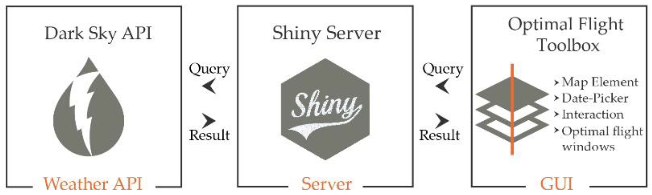
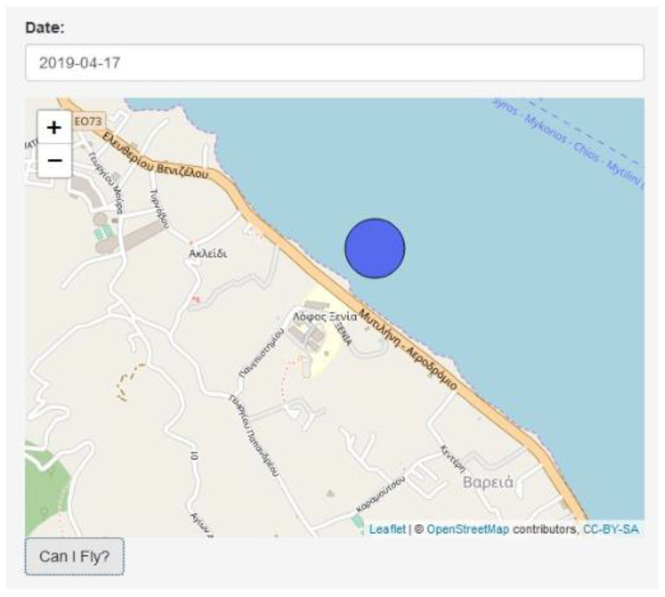
The architecture schema of the optimal flight toolbox is depicted in Figure 1 and consists of three fundamental components: (a) the GUI (Graphical User Interface), (b) the shiny Server, and (c) the Dark Sky Weather Application Programming Interface (API) [49]. The application GUI is composed of three core elements: (i) the Leaflet JS Map element, (ii) the date-picker element, and (iii) the optimal flight windows element. Through the map element, the users can identify the area of interest, to select the flight date using the date-picker and then submit the query through the Shiny server to the weather API (Figure 2). The submission process returns the results of the optimal flight windows element. The weather data was included using Dark sky application which is an award-winning application for accurate daily/hourly/minutely weather forecasting/prediction and visualization. Given the location, Dark Sky API utilizes a wide range of weather data sources such as NOAA’s GFS, German Meteorological Office and many others (https://darksky.net/dev/docs/sources), to serve the most accurate forecast possible. It offers up to 1000 free API requests per day and the query results are available in JavaScript Object Notation (JSON) file format.

Rules: Variables and Thresholds

Weather forecast data were used as hourly variables on which thresholds have been set to exclude outliers and values that are inconsistent. The thresholds were derived taking into consideration the theoretical protocol, the UAV specifications, and empirical data from many hours of flights and test missions. The proposed variables and thresholds compose the core rule set of the UAS toolbox.

In this ruleset the meteorological parameters temperature, wind speed, precipitation probability, humidity, and cloud coverage were calculated from Weather API that generates an hourly short-term (4 days) prediction. The wave height value is calculated using wind speed according to the Beaufort wind scale. Sun angle/elevation information is retrieved from the OCE library [50] which is a package for oceanographic data analysis.

In

Table 2. Ruleset of the Unmanned Aerial Systems (UAS) toolbox.

Variable	Thresholds	Units
Wind Speed	≤3.3	m/sec
Precipitation Probability	<50	%
Temperature	<38	Celsius
Cloud Cover	<25	%
Wave Height	≤0.5	m
Sun Elevation angle	25–45	degrees

the theoretical thresholds that define the optimal values for each variable are depicted. The optimal values for wind speed have been calculated smaller or equal to 3.3 m/s which corresponds from calm to light breeze wind conditions. Optimal wind speed values match with a wave height smaller or equal to 0.5 m. A percentage below 50% for the probability of precipitation (POP) is acceptable as it refers to scattered conditions at the forecast area. An air temperature under 38 Celsius degrees is safe for the aircraft’s operation. A cloud cover under 25% doesn’t affect the illumination of the aerial images as the sky is mostly clear and sunny. A percentage of 25% is the mean value of no cloud cover at all (0%) and half of the sky covered with clouds (50%). A cloud cover from 0 to 25% seems ideal for a marine survey so that the seabed is correctly illuminated. As for the sun elevation angle, it is recommended [21,28] that an angle between 25 to 45 degrees from the horizon is acceptable to avoid sun glint while the illumination of images is not decreasing.

The development of the optimal flight toolbox necessitates the combination of the variables and the corresponding theoretical thresholds to create mathematical rules based on Logical Conjunction and Set Theory. The theoretical thresholds constitute a set of optimal flight conditions (A) and the meteorological/environmental parameters are independent sets of predicted/expected values (B, C, D, E, F, G, H). Optimal flight conditions consider the intersection between the latter and the former values as mandatory. Equation 1 shows the mathematical formulation on which the optimal flight toolbox depends on. The results of the mathematical expression are binary (0, 1). Zero value stands for FALSE for no-optimal flight conditions and value one stands for TRUE for optimal flight conditions.

(A∩B) ∧ (A∩C) ∧ (A∩D) ∧ (A∩E) ∧ (A∩F) ∧ (A∩G) ∧ (A∩H)

(1)

3. Results

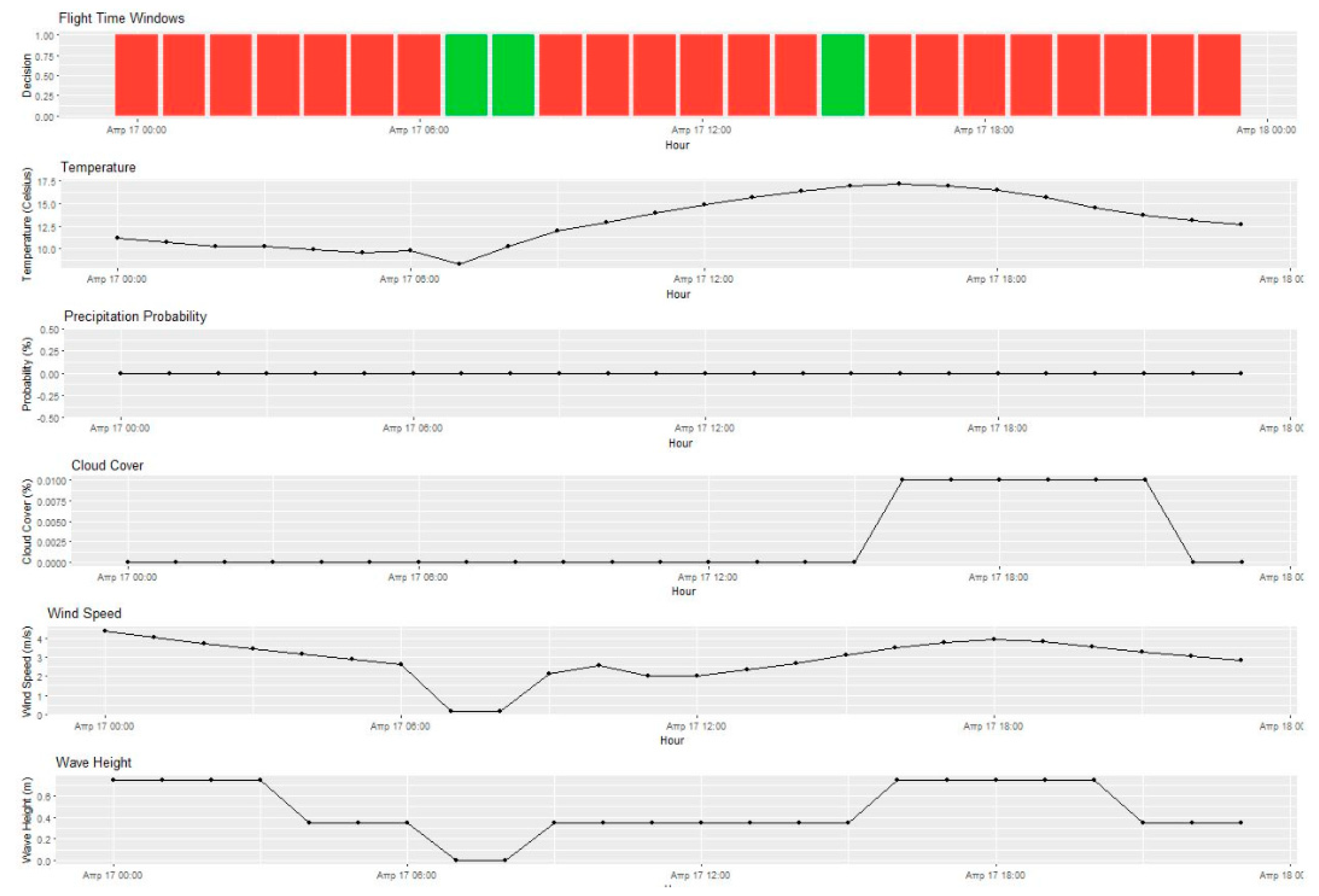
The UAS toolbox was used with the proposed ruleset at a coastal area and calculated the optimal flight window times on a picked day. The results of the UAS toolbox are presented through the optimal flight windows element which is shown in Figure 3, in a test site on a specific day. The bar at the top shows in red the false responses of the calculation which match with non-optimal flight conditions and in green the true responses which correspond to the optimal flight conditions, on that day. On the selected day, the proposed flight times are between 7:00 and 8:00 a.m. and at 3:00 p.m., while the hours of the rest of the day are not suggested for a flight survey, at the selected area. The graphs below the bar show the values of the variables (temperature, precipitation, cloud cover, wind speed, wave height) per hour. In Figure 3, it is apparent that the temperature on this day varies from 10 to 17 Celsius degrees, the precipitation probability is zero, the cloud cover varies from 0 to 10 percent, the top wind speed value is 4 m/s and the biggest wave height is 0.7 m. Considering the parameter values it is noticed that on the proposed flight times that day, between 7:00 and 8:00 a.m., both wind speed and wave height values are 0 and at 3:00 p.m. the wind speed is lower than 3 m/s and the wave height from 0.4 to 0.5m. These values are lower than the proposed thresholds and acceptable for data acquisition flight, therefore the positive result on these times of the day is considered as acceptable.

3.1. Case Studies

The next step for testing the UAS toolbox was its performance in the real world. We have applied the UAS toolbox on two days with diverse weather conditions, to check its validity and performance. On the first day, we chose a flight time that the conditions were optimal for marine data acquisition while on the second day the conditions of the chosen flight time were prohibitive due to the results of the toolbox. The reason, that those two case studies were chosen to test the toolbox, was to compare the data and conclude whether optimal flight conditions affect the quality of the acquired data.

The acquired aerial images of the two case studies were processed with the use of Structure from Motion (SfM) algorithms for the creation of orthophoto maps of the study area. The produced orthophoto maps seem to agree to the results of the UAS toolbox.

The selected study area is a coastal area in the middle east part of Lesvos Island which is located in the northeastern Aegean Sea, in Greece. The climate of Lesvos Island is Mediterranean, with mild, rainy winters and hot, sunny summers. The mean annual temperature is about 18 °C and a mean annual rainfall at 750 mm. Moreover, snow and very low temperatures are rare environmental conditions. The study area was chosen due to the interesting seabed which hosts different marine habitats and its position in the open sea which exposes it to a variety of weather conditions.

The UAS toolbox was used a day before each flight mission for more accurate weather predictions and was tested in different weather conditions and times (day and hour). The same flight plan was used for both case studies. A Phantom 4 Pro drone was used for the image acquisition at a flight altitude of 90 m and an image overlap at 80–70%. The direction of the flight was adapted to the sun azimuth angle to avoid sun glint.

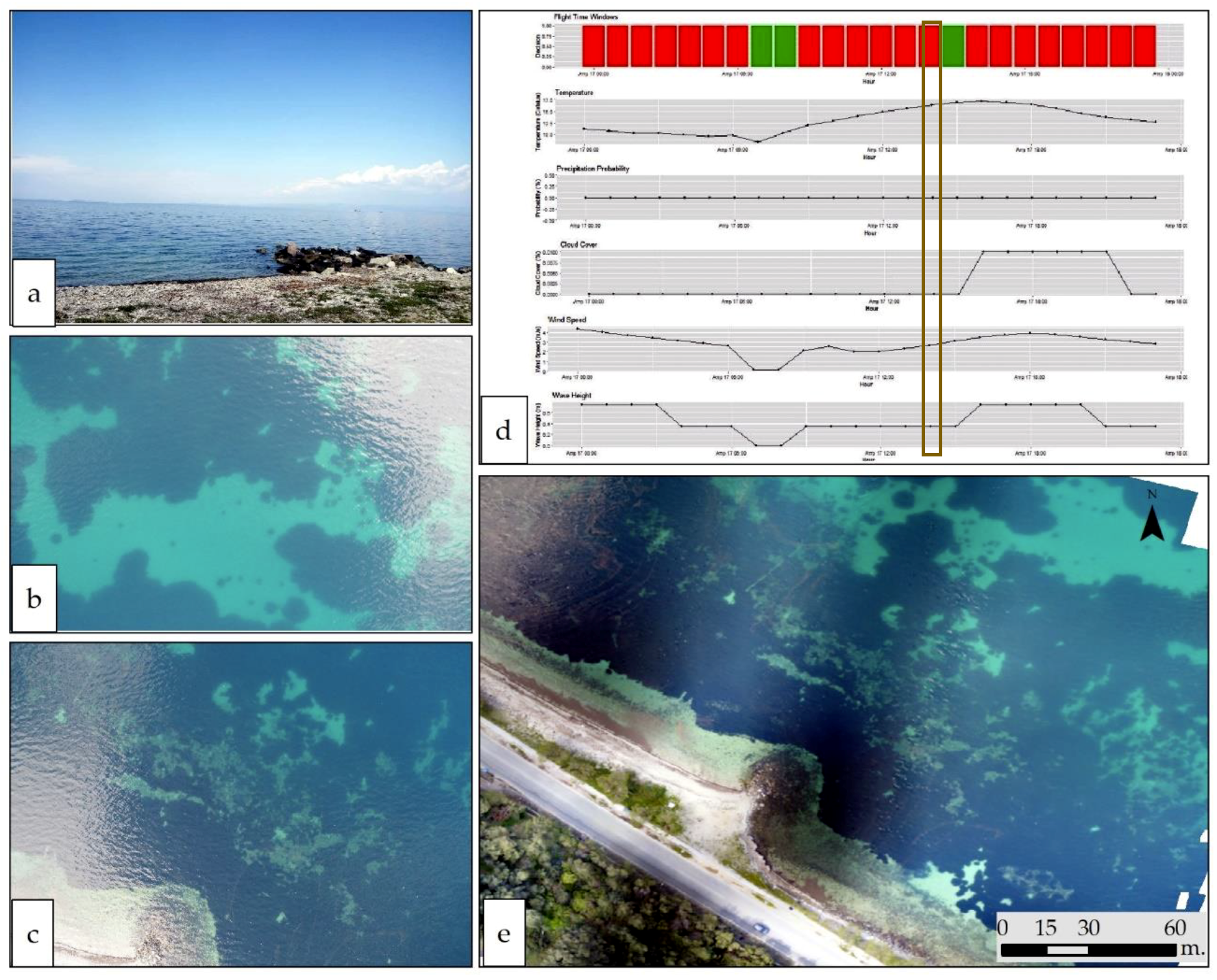
The first flight was performed on 17/04/19, at 3:38 pm as the prediction was positive on that day between 3:00 and 4:00 pm, as it is shown in Figure 4. At that time the elevation angle was calculated at 46.97 degrees, the sky was clear and according to Dark sky forecasts, the air temperature was 17 °C, the humidity 44%, and the precipitation was 0%, the wind speed was 2 m/s, and the wave height calculated at 0.4m. The values of the weather conditions were within the thresholds that have been set in the toolbox, therefore the positive result is considered correct.

The acquired images on that day were clear with good brightness, however we didn’t avoid completely the presence of sun glint at the edges of the images. We assume that this is due to the calculated sun angle at the flight time which was bigger than the suggested one. The produced orthophoto map is clear, correctly illuminated, and allows the collection of marine information with great precision. The different habitats on the seabed can easily be distinguished and mapped.

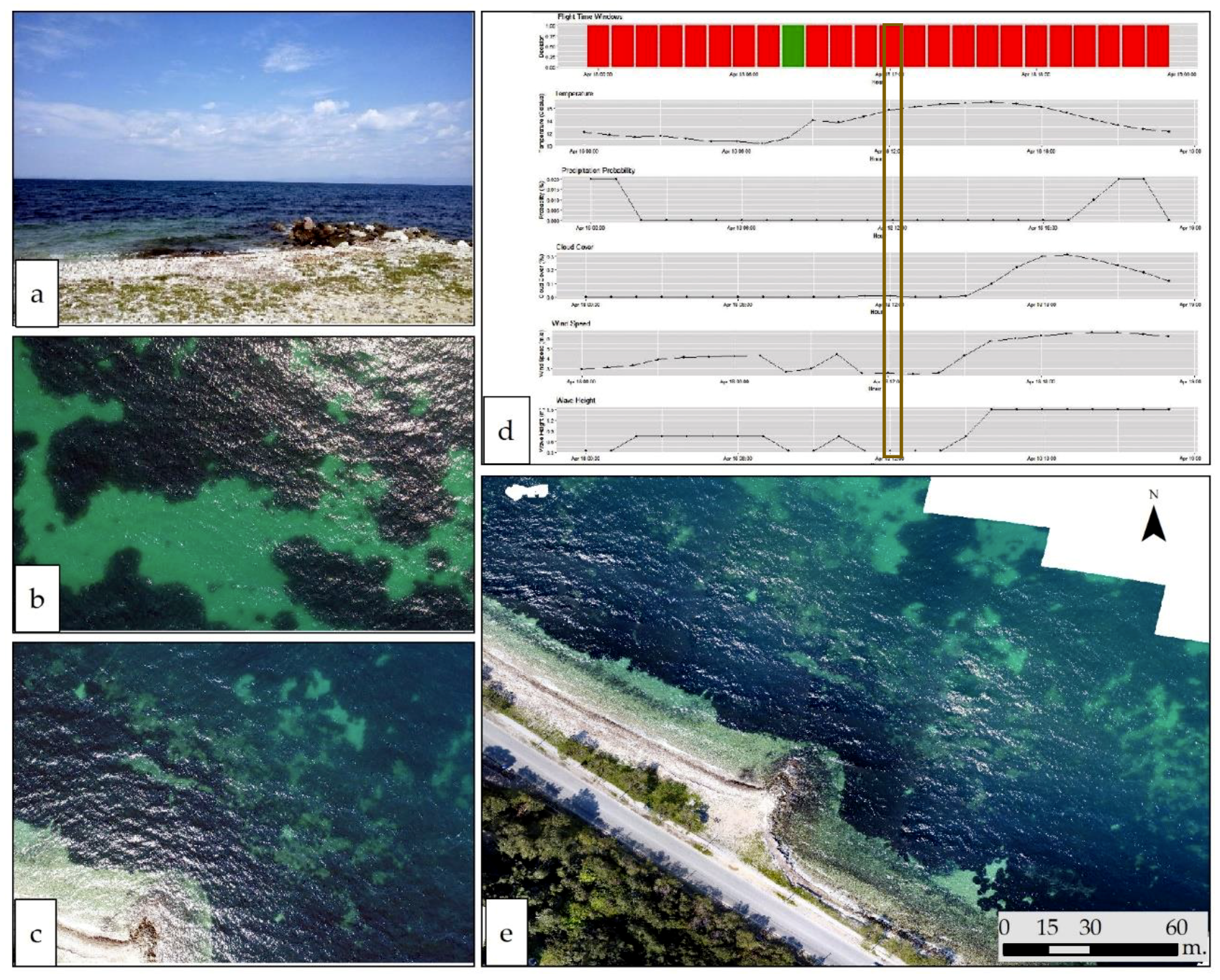
The second flight was performed on 18/04/19, at 2:36 pm, therefore, the prediction was not positive on that day, as it is shown in Figure 5. That flight time was chosen to compare the results of a non-optimal conditions flight with those of the previous day where the conditions were almost ideal.

At the selected flight time, the elevation angle was calculated at 56.25 degrees, the sky was partly cloudy and according to the forecasts, the air temperature was 18 °C, the humidity 39%, the precipitation was 0%, the wind speed was 6 m/s, and the wave height calculated at 1.09 m. The values of elevation angle, wind speed, and wave height were higher than the thresholds that have been set in the toolbox. This is the reason why the calculation for that time of the day was negative, according to the UAS toolbox.

The acquired images of the second case study had many differences from them of the first case study. As expected, the sea state is wavy which in combination with the sun glint effect have created white areas on parts of the images which prevent the visibility of the seabed. Furthermore, during the processing of the aerial images using SfM, some of the images couldn’t be aligned, resulting in missing information on the orthophoto map. The produced orthophoto map has low quality due to the wavy sea surface which doesn’t allow the detection and distinction of the marine habitats.

3.2. Comparison—Change Detection

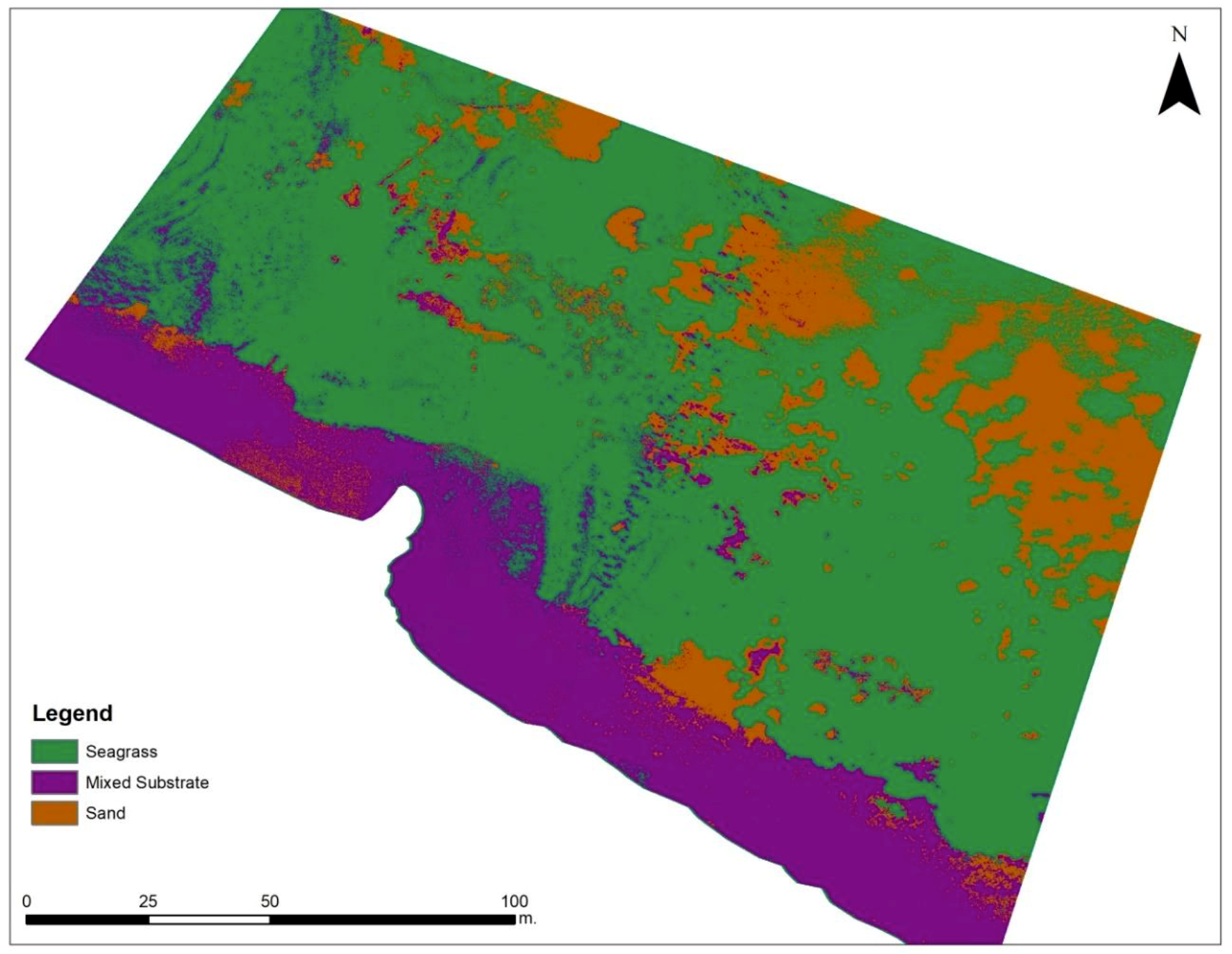
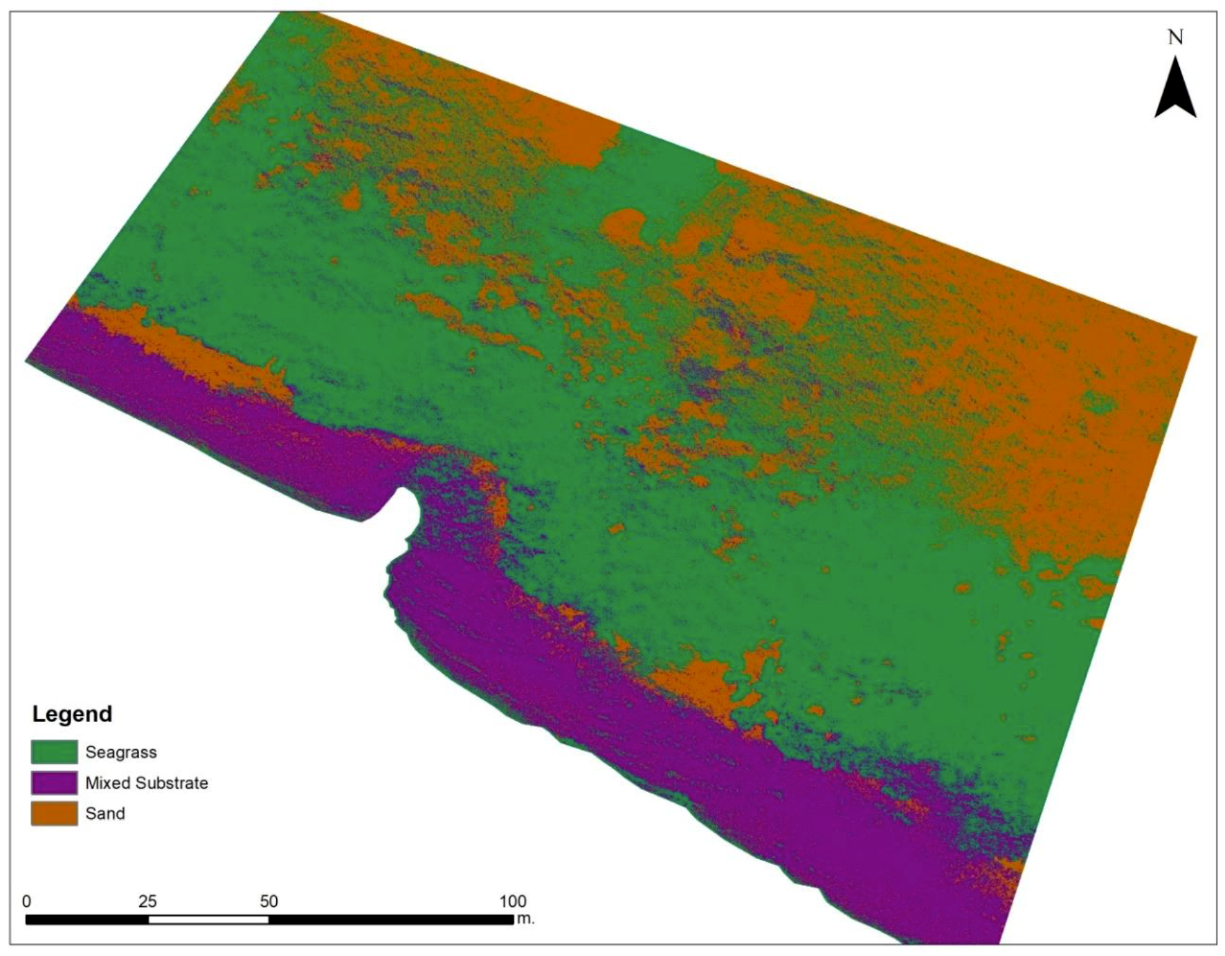
In order to compare and validate the results of the toolbox between the two case studies, a supervised classification method was applied on the produced orthophoto maps. The orthophoto maps were cropped to cover the same area and a land mask was applied. The chosen classes for the classification were seagrass, mixed substrate, and sand which are visible throughout the area. The same polygon areas have been used as training data in both classifications, so the classified maps can be comparable.

In the first case study (optimal conditions), the classification has a total accuracy of 94.4% and a K index of 0.92. The map of the first classification is shown in Figure 6, where 48.03% is covered by seagrass, 27.88% is mixed substrate, and 24.09% sand areas. The distinction of the classes is very clear.

In the second case study (non-optimal conditions), the classification has a total accuracy of 88.9% and a K index of 0.83. As it is shown in Figure 7, the habitat delineation in the non-optimal conditions map is not as clear as in the first case study and there are differences in classes coverages. The seagrass covers 43.39%, mixed substrate 26.87%, and sand 29.74% of the classified map. We assume that this is due to the wave presence and the sun glint areas of the second orthophoto map. Moreover, there are accuracy differences between the two classifications, which are 5.5% in total accuracy and 0.09 in the K index.

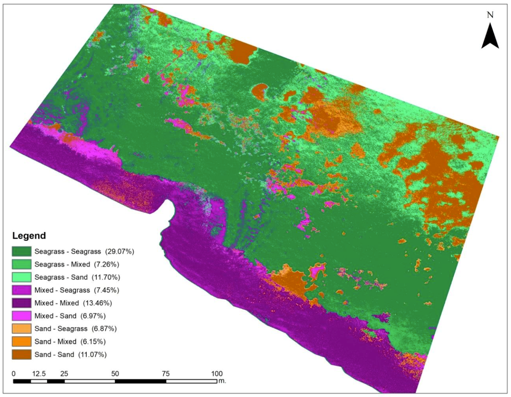
A change detection method on the classified maps showed quantitative changes of the three classes. The classified map of the first case study has been used as a reference map. The result of the comparison between optimal and non-optimal survey maps is shown in Figure 8, where the habitats that remained the same, in both cases, are presented in deeper color shades while the changed areas are presented in lighter color shades. For example, the areas of seagrass that have remained the same in both classifications, are presented in deep green and the percentage of them is 29.07%. A percentage of 7.26% of seagrass has changed in the mixed substrate and 11.70% of seagrass has changed in sandy areas. Similarly, 13.46% of the mixed substrate has remained the same, 7.45% of the mixed substrate has changed in seagrass, and 6.97% of the mixed substrate has changed into sand. As for the sand class, 11.07% has remained the same, 6.87% has changed in seagrass, and 6.15% has changed into mixed substrate.

The change detection results showed that there are few differences between the classification maps of the same area, on an optimal survey day and a non-optimal survey day. The coverage of seagrass has decreased by 10% and mixed substrate by 4% while the sand areas have increased by 23% in the second map. These differences are due to the presence of waves and sun glint at the second case study. Although, the percentages of changes are small in this comparison, they can cause wrong estimations in cases where high accuracy is required.

4. Discussion

The performance of a UAS toolbox has been tested and validated using two case studies over a coastal area. The UAS survey plan and the study area were the same in both case studies. The first UAS survey was performed under optimal flight conditions and the second under non-optimal flight conditions, according to the UAS toolbox. The results revealed that the acquired images and the produced orthophoto maps have significant differences in quality and acquired information. In the first case study, the orthophoto map is clear and allows the distinction of marine habitats, while the second orthophoto map includes less information due to non-alignment issues during the SfM process and low visibility of the seabed as a result of the wavy sea surface and sun glint areas. The results of the UAS toolbox showed that it can contribute to proper flight planning over coastal areas, save time from data acquisition and can be used in short-term planning with forecast data which are available globally for short periods. Moreover, a change detection method was applied on the classified orthophoto maps of the case studies, to collect quantitate comparison results between them. The results showed that there are few differences between the classification maps of the same area, on an optimal survey day and a non-optimal survey day. The results of the change detection demonstrate the value of the toolbox and the importance of following optimal survey conditions for the acquisition of reliable marine data using UAS.

The development of the optimal flight toolbox lays on the existence of open environmental and marine data and the computational power and open-source character of R programming language. While Dark Sky API seems to be a promising application for weather forecast/prediction there is a lack of specialization in oceanographic conditions and parameters.

The ruleset of the toolbox includes the meteorological parameters, temperature, wind speed, precipitation probability, humidity, and cloud coverage which are available by the Dark Sky API for short-term prediction, wave height calculated using wind speed, as wave forecast data aren’t available in high resolution and sun angle information which is retrieved from the OCE library package. The proposed thresholds of these parameters were derived taking into consideration the theoretical protocol, the UAV specifications, and personal experience of UAS flights and test missions. These thresholds have been effective for us in the past and are suggested to other users. Additionally, in the final version of the UAS toolbox, it is planned that the thresholds will be adjustable by the users. As the forecast data are available for short term prediction, the UAS toolbox can be used only in short-term planning surveys.

In long-term planning, the collection of time series of parameters like turbidity levels, phenology, wind speed patterns, will be useful to gather knowledge of the conditions prevailing in the study area per season and subsequently can lead to conclusions of the optimal season of year and time of day to operate a UAV flight. In addition, the collection of in-situ data in the study area provides complementary information on oceanographic parameters that in combination with aerial observations completes a successful UAS survey in coastal areas.

A UAS data acquisition protocol in coastal areas is proposed in this study. The proposed UAS protocol summarizes the parameters that affect the collection of reliable high-resolution images in the marine environment and can be used in a wide range of oceanographic applications. The parameters of the protocol have been grouped considering existing protocols for aerial photography [21,22], UAS limitations in marine applications [20] and personal experience in flight planning using UAS, in three main categories: (i) Morphology of the area, (ii) Environmental conditions, (iii) Flight parameters. Although the limitations of UAS data acquisition over the sea have been reported in many applications [22,24], it is the first time that a dedicated protocol for UAS data acquisition in coastal areas is presented.

5. Conclusions

A UAS data acquisition protocol for aerial survey in coastal areas has been presented in this study. Although, UAS has been used recently in coastal and marine applications, their ability in collecting accurate and quality data deals with some limitations. These limitations refer to environmental parameters, sea state conditions, and flight planning parameters that affect the quality and reliability of the acquired data. The identification and categorization of the parameters that affect the acquired data are essential for the collection of high-resolution information in marine applications with the use of UAS. Thus, a UAS protocol is necessary for an effective UAV flight survey over coastal areas. To the best of our knowledge, the proposed data acquisition protocol is the first report of a protocol for marine data acquisition using UAS.

Furthermore, a UAS toolbox for the calculation of optimal flight time windows has been developed, with the use of the open-source R programming language and forecast weather data from the Dark Sky API. The parameters temperature, wind speed, precipitation probability, humidity, cloud coverage, wave height, and sun angle have been used as inputs in the toolbox. These parameters in combination with theoretical thresholds that have been set on their values constitute the ruleset of the toolbox.

The UAS toolbox has been tested in two case studies, optimal and non-optimal conditions surveys, where the results showed significant differences in the quality of the acquired information. Moreover, a comparison between the classified maps of the case studies was performed, where the quantitate results were calculated. The results showed classification accuracy differences and underestimation of some habitats in the area at the non-optimal survey day, because of wave presence and sun glint areas.

Concluding, the proposed UAS protocol improves the quality of the acquired data, saves the time of the survey plan, and represents an effective methodology for marine data acquisition. Additionally, the UAS toolbox as an easy to use tool improves the flight planning of a UAS survey and results in the acquisition of high-resolution oceanographic and marine data. These results can lead to the collection of the necessary data for the protection and management of the marine ecosystems.

References

- Hedley, J.D.; Roelfsema, C.M.; Chollett, I.; Harborne, A.R.; Heron, S.F.; Weeks, S.J.; Skirving, W.J.; Strong, A.E.; Eakin, C.M.; Christensen, T.R.L.; et al. Remote Sensing of Coral Reefs for Monitoring and Management: A Review. Remote Sens. 2016, 8, 118. [Google Scholar] [CrossRef]
- Topouzelis, K.; Spondylidis, S.C.; Papakonstantinou, A.; Soulakellis, N. The use of Sentinel-2 Imagery for Seagrass Mapping: Kalloni Gulf (Lesvos Island, Greece) Case Study. In Proceedings of the Fourth International Conference on Remote Sensing and Geoinformation of the Environment (RSCy2016), At Paphos, Cyprus, 4–8 April 2016. [Google Scholar] [CrossRef]
- Topouzelis, K.; Makri, D.; Stoupas, N.; Papakonstantinou, A.; Katsanevakis, S. Seagrass mapping in Greek territorial waters using Landsat-8 satellite images. Int. J. Appl. Earth Obs. Geoinf. 2018, 67, 98–113. [Google Scholar] [CrossRef]
- Ventura, D.; Bruno, M.; Lasinio, G.J.; Belluscio, A.; Ardizzone, G. A low-cost drone based application for identifying and mapping of coastal fish nursery grounds. Estuar. Coast. Shelf Sci. 2016, 171, 85–98. [Google Scholar] [CrossRef]
- Harper, J.R.; Morris, M.; Daley, S. OREGON SHOREZONE Coastal Habitat Mapping Protocol. Available online: http://www.shorezone.org/documents/OregonProtocol_Final_July2014.pdf (accessed on 24 June 2019).
- Hodgson, A.; Kelly, N.; Peel, D. Unmanned aerial vehicles (UAVs) for surveying Marine Fauna: A dugong case study. PLoS ONE 2013, 8, e79556. [Google Scholar] [CrossRef] [PubMed]
- Burns, J.; Delparte, D.; Gates, R. Takabayashi Integrating structure-from-motion photogrammetry with geospatial software as a novel technique for quantifying 3D ecological characteristics of coral reefs. PeerJ 2015, 3, e1077. [Google Scholar] [CrossRef] [PubMed]
- Casella, E.; Collin, A.; Harris, D.; Ferse, S.; Bejarano, S.; Parravicini, V.; Hench, J.L.; Rovere, A. Mapping coral reefs using consumer-grade drones and structure from motion photogrammetry techniques. Coral Reefs 2017, 36, 269–275. [Google Scholar] [CrossRef]
- Turner, I.L.; Harley, M.D.; Drummond, C.D. UAVs for coastal surveying. Coast. Eng. 2016, 114, 19–24. [Google Scholar] [CrossRef]
- Topouzelis, K.; Papakonstantinou, A.; Pavlogeorgatos, G. Coastline Change Detection Using UAV, Remote Sensing, GIS and 3D Reconstruction. In Proceedings of the 5th International Conference on Environmental Management, Engineering, Planning and Economics (CEMEPE) and SECOTOX Conference, Mykonos Island, Greece, 14–18 June 2015. [Google Scholar]
- Ferrari, R.; McKinnon, D.; He, H.; Smith, R.; Corke, P.; González-Rivero, M.; Mumby, P.; Upcroft, B. Quantifying multiscale habitat structural complexity: A cost-effective framework for underwater 3D modelling. Remote Sens. 2016, 8, 113. [Google Scholar] [CrossRef]
- Papakonstantinou, A.; Topouzelis, K.; Pavlogeorgatos, G. Coastline Zones Identification and 3D Coastal Mapping Using UAV Spatial Data. ISPRS Int. J. Geo-Inf. 2016, 5, 75. [Google Scholar] [CrossRef]
- Topouzelis, K.; Papakonstantinou, A.; Doukari, M.; Stamatis, P.; Makri, D.; Katsanevakis, S. Coastal Habitat Mapping in the Aegean Sea Using High Resolution Orthophotomaps. In Proceedings of the Fifth International Conference on Remote Sensing and Geoinformation of the Environment (RSCy2017), Paphos, Cyprus, 20–23 March 2017. [Google Scholar]
- Makri, D.; Stamatis, P.; Doukari, M.; Papakonstantinou, A.; Vasilakos, C.; Topouzelis, K. Multi–Scale Seagrass Mapping in Satellite Data and the Use of UAV in Accuracy Assessment. In Proceedings of the Sixth International Conference on Remote Sensing and Geoinformation of Environment (RSCy2018), Paphos, Cyprus, 26–29 March 2018. [Google Scholar]
- Topouzelis, K.; Papakonstantinou, A.; Garaba, S.P. Detection of floating plastics from satellite and unmanned aerial systems (Plastic Litter Project 2018). Int. J. Appl. Earth Obs. Geoinf. 2019, 79, 175–183. [Google Scholar] [CrossRef]
- Topouzelis, K.; Papakonstantinou, A.; Doukari, M. Coastline change detection using Unmanned aerial vehicles and image processing techniques. Fresenius Environ. Bull. 2017, 26, 5564–5571. [Google Scholar]
- Papakonstantinou, A.; Doukari, M.; Stamatis, P.; Topouzelis, K. Coastal Management using UAS and High-Resolution Satellite Images for Touristic Areas. Int. J. Appl. Geospat. Res. 2017, 10, 54–72. [Google Scholar] [CrossRef]
- Mancini, F.; Dubbini, M.; Gattelli, M.; Stecchi, F.; Fabbri, S.; Gabbianelli, G. Using Unmanned Aerial Vehicles (UAV) for High-Resolution Reconstruction of Topography: The Structure from Motion Approach on Coastal Environments. Remote Sens. 2013, 5, 6880–6898. [Google Scholar] [CrossRef] [Green Version]
- Long, N.; Millescamps, B.; Guillot, B.; Pouget, F.; Bertin, X. Monitoring the Topography of a Dynamic Tidal Inlet Using UAV Imagery. Remote Sens. 2016, 8, 387. [Google Scholar] [CrossRef]
- Doukari, M.; Papakonstantinou, A.; Topouzelis, K. Preview of a Protocol for UAV Data Collection in Coastal Areas. In Proceedings of the Sixth International Conference on Remote Sensing and Geoinformation of Environment (RSCy2018), Paphos, Cyprus, 26–29 March 2018. [Google Scholar]
- Finkbeiner, M.; Stevenson, B.; Seaman, R. Guidance for Benthic Habitat Mapping: An Aerial Photographic Approach, Control; NOAA/CSC/20117-PUB; NOAA/National Ocean Service/Coastal Services Center: Charleston, SC, USA, 2001; p. 75.
- Coggan, R.; Populus, J.; White, J.; Sheehan, K.; Fitzpatrick, F.; Piel, S. (Eds.) Review of Standards and Protocols for Seabed Habitat Mapping; MESH: Peterborough, UK, 2007; Available online: http://www.emodnet-seabedhabitats.eu/default. aspx?page=1442 (accessed on 1 November 2016).
- Hogg, O.T.; Huvenne, V.A.I.; Griffiths, H.J.; Dorschel, B.; Linse, K. Landscape mapping at sub-Antarctic South Georgia provides a protocol for underpinning large-scale marine protected areas. Sci. Rep. 2016, 6, 33163. [Google Scholar] [CrossRef] [Green Version]
- Guihen, D.; Robst, J.; Crofts, S.; Stanworth, A.; Enderlein, P.; Ratcliffe, N. A protocol for the aerial survey of penguin colonies using UAVs. J. Unmanned Veh. Syst. 2015, 3, 95–101. [Google Scholar] [Green Version]
- Deidun, A.; Gauci, A.; Lagorio, S.; Galgani, F. Optimising beached litter monitoring protocols through aerial imagery. Mar. Pollut. Bull. 2018, 131, 212–217. [Google Scholar] [CrossRef]
- Topouzelis, K.N. Oil Spill Detection by SAR Images: Dark Formation Detection, Feature Extraction and Classification Algorithms. Sensors 2008, 8, 6642–6659. [Google Scholar] [CrossRef] [Green Version]
- Topouzelis, K.; Kitsiou, D. Detection and classification of mesoscale atmospheric phenomena above sea in SAR imagery. Remote Sens. Environ. 2015, 160, 263–272. [Google Scholar] [CrossRef]
- Mount, R. Acquisition of Through-water Aerial Survey Images: Surface Effects and the Prediction of Sun Glitter and Subsurface Illumination. Photogramm. Eng. Remote Sens. 2005, 71, 1407–1415. [Google Scholar] [CrossRef]
- Joyce, K.E.; Duce, S.; Leahy, S.M.; Leon, J.; Maier, S.W. Principles and practice of acquiring drone-based image data in marine environments. Mar. Freshw. Res. 2018, 70, 952–963. [Google Scholar] [CrossRef]
- Wang, M.; Bailey, S.W. Correction of the Sunglint Contamination on the SeaWiFS Aerosol Optical Thickness Retrievals. SeaWiFS Postlaunch Tech. Rep. Ser. 2000, 9, 65–69. [Google Scholar]
- Hochberg, E.J.; Andréfouët, S.; Tyler, M.R. Sea surface correction of high spatial resolution ikonos images to improve bottom mapping in near-shore environments. IEEE Trans. Geosci. Remote Sens. 2003, 41, 1724–1729. [Google Scholar] [CrossRef]
- Hedley, J.D.; Harborne, A.R.; Mumby, P.J. Simple and robust removal of sun glint for mapping shallow-water benthos. Int. J. Remote Sens. 2005, 26, 2107–2112. [Google Scholar] [CrossRef]
- Leng, F.; Tan, C.M.; Pecht, M. Effect of Temperature on the Aging rate of Li Ion Battery Operating above Room Temperature. Sci. Rep. 2015, 5, 12967. [Google Scholar] [CrossRef] [PubMed] [Green Version]
- Dogliotti, A.; Ruddick, K.; Nechad, B.; Doxaran, D.; Knaeps, E. A single algorithm to retrieve turbidity from remotely-sensed data in all coastal and estuarine waters. Remote Sens. Environ. 2015, 156, 157–168. [Google Scholar] [CrossRef] [Green Version]
- Barker, S. Maine Eelgrass Mapping Protocol; Report for the Casco Bay Estuary Partnership and the Maine Depth of Environmental Protection; Casco Bay Estuary Partnership: Portland, ME, USA, 2015; Available online: https://www.cascobayestuary.org/wp-content/uploads/2018/02/Maine-Eelgrass-Mapping-Protocol-Barker-2015.pdf (accessed on 24 June 2019).
- Fiedler, P.C. Comparison of objective descriptions of the thermocline. Limnol. Oceanogr. Methods 2010, 8, 313–325. [Google Scholar] [CrossRef]
- Elçi, Ş. Effects of thermal stratification and mixing on reservoir water quality. Limnology 2008, 9, 135–142. [Google Scholar] [CrossRef] [Green Version]
- Akbari, E.; Alavipanah, S.K.; Jeihouni, M.; Hajeb, M.; Haase, D.; Alavipanah, S. A Review of Ocean/Sea Subsurface Water Temperature Studies from Remote Sensing and Non-Remote Sensing Methods. Water 2017, 9, 936. [Google Scholar] [CrossRef]
- Diaz-Almela, E.; Marbà, N.; Álvarez, E.; Balestri, E.; Ruiz-Fernández, J.M.; Duarte, C.M. Patterns of seagrass (Posidonia oceanica) flowering in the Western Mediterranean. Mar. Biol. 2006, 148, 723–742. [Google Scholar] [CrossRef]
- Austin, R. Unmanned Aircraft Systems: UAVS Design, Development and Deployment; John Wiley & Sons Inc.: New York, NY, USA, 2009. [Google Scholar]
- Papakonstantinou, A.; Doukari, M.; Moustakas, A.; Chrisovalantis, D.; Chaidas, K.; Roussou, O.; Athanasis, N.; Topouzelis, K.; Soulakellis, N. UAS Multi-Camera rig for Post-Earthquake Damage 3D Geovisualization of Vrisa village. In Proceedings of the Sixth International Conference on Remote Sensing and Geoinformation of Environment (RSCy2018), Paphos, Cyprus, 26–29 March 2018. [Google Scholar]
- O’Connor, J.; Smith, M.J.; James, M.R. Cameras and settings for aerial surveys in the geosciences: Optimising image data. Prog. Phys. Geogr. 2017, 41, 325–344. [Google Scholar] [CrossRef]
- O’Connor, J.; Smith, M. A Review of Cameras Popular Amongst Aerial Surveyors. Available online: www.prodrone-tech.com (accessed on 20 June 2019).
- Pix4D. Pix4Dcapture: Free Drone Flight Planning Mobile App; Pix4D: Lausanne, Switzerland, 2011; Available online: https://www.pix4d.com/product/pix4dcapture (accessed on 20 June 2019).
- Mission Planner Home—Mission Planner Documentation. 2016. Available online: http://ardupilot.org/planner/ (accessed on 20 June 2019).
- Kakaes, K.; Greenwood, F.; Lippincot, M.; Dosemagen, S.; Meier, P.; Wich, S. Drones and Aerial Observation: New Technologies for Property Rights, Human Rights, and Global Development: A Primer. 2015. Available online: http://www.rhinoresourcecenter.com/pdf_files/143/1438073140.pdf (accessed on 24 June 2019).
- R Core Team. R: A Language and Environment for Statistical Computing; R Foundation for Statistical Computing: Vienna, Austria, 2016; Available online: http://www.R-project.org/ (accessed on 25 June2019).
- Studio, I.R. Easy Web Applications in R; RStudio Inc.: Boston, MA, USA, 2013. [Google Scholar]
- The Dark Sky Company. 2011. Available online: https://darksky.net (accessed on 25 June2019).
- Kelley, D. “The oce Package”, in Oceanographic Analysis with R; Springer: New York, NY, USA, 2018; pp. 91–101. [Google Scholar]
© 2019 by the authors. Licensee MDPI, Basel, Switzerland. This article is an open access article distributed under the terms and conditions of the Creative Commons Attribution (CC BY) license (http://creativecommons.org/licenses/by/4.0/).