Article

The Consistency of SSM/I vs. SSMIS and the Influence on Snow Cover Detection and Snow Depth Estimation over China

1
State Key Laboratory of Remote Sensing Science, Jointly Sponsored by Beijing Normal University and Institute of Remote Sensing and Digital Earth of Chinese Academy of Sciences, Beijing Engineering Research Center for Global Land Remote Sensing Products, Faculty of Geographical Science, Beijing Normal University, Beijing 100875, China
2
Key Laboratory of Remote Sensing of Gansu Province, Heihe Remote Sensing Experimental Research Station, Cold and Arid Regions Environmental and Engineering Research Institute, Chinese Academy of Sciences, Lanzhou 730000, China
3
State Key Laboratory of Remote Sensing Science, Institute of Remote Sensing and Digital Earth, Aerospace Information Research Institute, Chinese Academy of Sciences, Beijing 100010, China
4
National Satellite Meteorological Center, China Meteorological Administration, Beijing 100081, China
*
Author to whom correspondence should be addressed.
Remote Sens. 2019, 11(16), 1879; https://doi.org/10.3390/rs11161879
Submission received: 13 June 2019 / Revised: 7 August 2019 / Accepted: 8 August 2019 / Published: 11 August 2019

Abstract

:
The long-term variations in snow depth are important in hydrological, meteorological, and ecological implications and climatological studies. The series of Special Sensor Microwave/Imager (SSM/I) and Special Sensor Microwave Imager Sounder (SSMIS) instruments onboard the Defense Meteorological Satellite Program (DMSP) platforms has provided a consistent 30+ year data record of global observations that is well-suited for the estimation of snow cover, snow depth, and snow water equivalent (SWE). To maximize the use of this continuous microwave observation dataset in long-term snow analysis and obtain an objective result, consistency among the SSM/I and SSMIS sensors is required. In this paper, we evaluated the consistency between the SSM/I and SSMIS concerning the observed brightness temperature (Tb) and the retrieved snow cover area and snow depth from January 2007 to December 2008, where the F13 SSM/I and the F17 SSMIS overlapped. Results showed that Tb bias at 19 GHz spans from −2 to −3 K in snow winter seasons, and from −4 to −5 K in non-snow seasons. There is a slight Tb bias at 37 GHz from −2 to 2 K, regardless of season. For 85 (91) GHz, the bias presents some uncertainty from the scattering effect of the snowpack and atmospheric emission. The overall consistency between SSM/I and SSMIS with respect to snow cover detection is between 80% and 100%, which will result in a maximum snow cover area difference of 25 × 104 km2 in China. The inconsistency in Tb between SSM/I and SSMIS can result in a −2 and −0.67 cm snow depth bias for the dual-channel and multichannel algorithms, respectively. SSMIS tends to yield lower snow depth estimates than SSM/I. Moreover, there are notable bias differences between SSM/I- and SSMIS-estimated snow depths in the tundra and taiga snow classes. Our results indicate the importance of considering the Tb bias in microwave snow cover detection and snow depth retrieval and point out that, due to the sensitivity of bias to seasons, it is better to do the intercalibration with a focus on snow-covered winter seasons. Otherwise, the bias in summer will disturb the calibration coefficients and introduce more error into the snow retrievals if the seasonal difference is not carefully evaluated and separated.

1. Introduction

Seasonal snow covers a considerable portion of the land in the Northern Hemisphere during winter [1,2]. It plays an important role in the Earth’s hydrological cycle, energy balance, and climate system [1,2,3,4]. Long-term consistent snow cover records, including snow water equivalent (SWE), snow cover extent (SCE), and snow albedo (SA), are vital to initialize numerical weather prediction models, hydrologic models, and land surface process models over the Northern Hemisphere [5,6,7,8,9,10].
Manual snow surveys are time-consuming and expensive, and observations from widely spaced weather stations cannot represent the detailed spatial distribution of snow depth [11,12,13,14]. Fortunately, spaceborne passive microwave (PMW) sensors have proven to be valuable for monitoring snowpack distributions at global and regional scales [11,12,13,14,15]. Moreover, PMW is only lightly affected by weather conditions and its signals are sensitive to snow depth [11,12,13]. Therefore, it can be used to provide nearly real-time snow cover data [5,6,16,17]. These advantages make SWE estimation from satellite PMW remote sensing an attractive option.
A long archive of historical satellite data dating back to 1978 is another advantage of PMW, which consists of Scanning Multichannel Microwave Radiometer (SMMR, 1978−1987) data, Special Sensor Microwave/Imager (SSM/I, 1987−2009) data, and Special Sensor Microwave Imager/Sounder (SSMIS, 2006−the present) data from the U.S. Defense Meteorological Satellite Program (DMSP) satellites; and NASA’s Advanced Microwave Scanning Radiometer data for the Earth Observing System (AMSR-E, 2002–2011) to AMSR2 (2012−the present) [15,18,19,20]. The Microwave Radiation Imager (MWRI) onboard the Chinese FengYun-3 (FY-3) series of satellites (FY-3A, 2008; FY-3B, 2010−the present; FY-3C, 2013−the present; FY-3D, 2017−the present) was designed for broad meteorological and environmental applications [21]. Subsequent satellites FY-3E, 3F, and 3G are expected to be launched by 2025.
Among these sensors, SSM/I and SSMIS are preferable due to the long-term data (from 1987 to the present), serial satellite platforms (DMSP-F8, F11, F13, F17), and similar sensor specifications (passing time, frequency, and footprint). The European Space Agency GlobSnow project (http://www.globsnow.info/) has released the Version 2.0 SWE dataset from 1979 to the present for the Northern hemisphere [11,14,22,23]. The snow depth product from the West Data Center of China (WESTDC, http://westdc.westgis.ac.cn) was generated based on the modified Chang algorithm [24,25,26]. Satellite data used in these products are in the EASE-Grid equal-area projection with a nominal resolution of 25 km × 25 km from SMMR (1978−1987), SSM/I, and SSMIS (1987−the present) [15]. These snow products have been used in studies of climate change, hydrological processes, vegetation growth, permafrost changes, and river runoff [2,5,9,12,13,24,27,28].
However, numerous studies on the intercalibration of microwave radiometer brightness temperature (Tb) between SMMR and SSM/I(F08), SSM/I(F08) and SSM/I(F11), SSM/I(F11) and SSM/I(F13), SSMIS and AMSR-E (AMSR2), and AMSR-E (AMSR2) and FY-3B/C in various regions indicate that a large gap exists among different sensors and intercalibration could improve the long-term dataset consistency [15,24,29,30,31,32,33,34,35,36]. Generally, there are three methods for intercalibrating sensors, including the simultaneous nadir or conical overpass (SNO or SCO), statistical intercalibration, and double differencing (DD) methods [24,29,35,36,37,38]. An intercalibrated Fundamental Climate Data Record (FCDR) of brightness temperatures funded by the National Oceanographic and Atmospheric Administration (NOAA) has been developed using data from a series of DMSP radiometers [16]. The results indicate that although the SSM/I and SSMIS instruments are “identical” copies, there are significant differences in Tb between the sensors. Although some evaluations have been conducted on the consistency between SSM/I and SSMIS, few have been done on the consistency of the snow depth and snow cover extent derived from these sensors. Dai et al. (2015) developed a technique for inter-sensor calibration between SSM/I and SSMIS [24]. The calibration improved the relative biases in the snow cover extent and snow volume from 42.42% to 1.65%, and from 66.18% to −1.5%, respectively. In the paper, they regarded a pixel as snow cover if the brightness temperature difference (19−37 GHz) was greater than 0, rather than using PMW snow cover mapping algorithms. The snow depth was derived with the modified Chang algorithm, which only uses 19 and 37 GHz at horizontal polarization. Cho et al. (2017) evaluated the consistency of SWE retrievals from SSM/I and SSMIS over North Central United States [34]. The SWE estimates were retrieved from the Chang algorithm at 19 and 37 GHz frequencies. Results showed that there were notable SWE differences between the SSM/I and SSMIS sensors in the warm forest class. However, SWE differences between SSM/I and SSMIS were not directly compared with overlapping data but AMSR-E SWE was used as a baseline.
The assessment of the consistency of SSM/I vs. SSMIS is necessary because (a) beginning with the processing of the SSMIS sensor, EASE-Grid Tb fields are gridded using an inverse distance squared method instead of Backus-Gilbert interpolation, which had been used for the earlier SSM/I sensors; (b) SSMIS has the same seven channels with SSM/I, but the 85.5 GHz frequency was moved to 91.655 GHz; (c) the DMSP SSM/I-SSMIS Pathfinder Daily EASE-Grid Brightness Temperatures data have been widely used to generate time series snow products, such as GlobSnow and WESTDC, whose consistency is very important for scientific and applied purposes; (d) the inconsistency in Tb can result in different retrievals, such as snow cover area and snow depth, from SSM/I and SSMIS.
Thus, the main purpose of this paper is to assess the consistency of SSM/I and SSMIS in the overlapping time, including Tb, snow cover detection, and snow depth estimation. The three main goals of the paper are (1) to compare the Tbs from SSM/I and SSMIS, including 19, 37, and 85 (91) GHz. These channels are all sensitive to snow depth or SWE; (2) to determine the influence of SSM/I and SSMIS on PMW snow cover mapping algorithms. The snow cover detection is not only necessary to snow depth estimation but also determines the SCE; and (3) to evaluate the influence of Tb variation from SSM/I and SSMIS on snow depth estimation. The paper is organized as follows. Data and methodology are presented in Section 2. Section 3 describes the comparison between SSM/I and SSMIS, including Tb, snow cover, and snow depth. Section 4 discusses the influence of snow depth, seasons, seasonal snow classes, and intercalibration on the consistency between SSM/I and SSMIS. Section 5 is devoted to our conclusions.

2. Materials and Methods

2.1. Data

(1) Satellite passive microwave data
The SSM/I and SSMIS series sensors on the U.S. DMSP satellites collect continuous data at four frequencies (19, 22, 37, 85, or 91 GHz) from 1987 to the present. Both the vertical and horizontal polarizations are measured, except at 22 GHz, where only the vertical polarization is measured. The cold overpass data from all sensors are from descending orbits, except the SSM/I (F08). The radiometric characteristics of the SSM/I (F13) and SSMIS (F17) are listed in Table 1. The SSM/I sensor has three major differences from the SSMIS instrument, including (a) coarser footprint size; (b) slightly narrower orbital swath; and (c) channel difference (85.5 vs. 91.655 GHz).
The F13 SSM/I and F17 SSMIS sensors provided Tb measurements from May 1995 to March 2009 and from December 2006 to the present, respectively. The data are available from the National Snow and Ice Data Center (NSIDC, https://nsidc.org/data/NSIDC-0032). Although F17 SSMIS data is already cross-calibrated with SSM/I sensors in Remote Sensing Systems (RSS, V7), cross-calibration does not imply complete homogenization across sensors [15]. There are more than two years overlapping, and these can be used to study the consistency between SSM/I (F13) and SSMIS (F17) at the same place and similar overpass time. In this study, we conduct an intercomparison of F13 with F17 data from 1 January 2007 through 31 December 2008. To avoid the influence of wet snow, only descending overpass data were used.
(2) In situ snow depth measurement
The weather station data were acquired from the National Meteorological Information Centre, China Meteorology Administration (http://www.cma.gov.cn/). The dataset of snow depth measurements used in this paper is from 753 stations throughout China (Figure 1, left) from 2007 to 2008. Recorded variables include the site name, observation time, geolocation (latitude and longitude), elevation (m), near-surface soil temperature (measured at a 5 cm depth, °C), and snow depth (cm). Quality control was conducted prior to the use of the data. The first step was to select records where the near-surface soil temperature was lower than 0 °C. The second step was to remove the sites if the areal fraction of the open water exceeds 30% in the satellite pixel.
(3) Land cover fraction and snow cover classification
A 1 km land use/land cover (LULC) map derived from the 30 m Thematic Mapper (TM) imagery classification was provided by the Data Center for Resources and Environmental Sciences, Chinese Academy of Sciences (http://www.resdc.cn/). Since the 1 km LULC map was derived from 30 m TM imagery, it can be recalculated as the areal percentage of each land cover type in the 25 km grid cells (Figure 1, left). In this study, the fractions of grassland, barren land, farmland, forest, and shrubland were calculated to analyze the land cover effects on Tb difference between SSM/I and SSMIS [39].
To consider major spatial characteristics related to snow cover, we studied the consistency in Tb and snow depth estimates in various climatological snow classes. Based on the seasonal snow classification system in [40], there are four major snow classes in China, including taiga, tundra, prairie, and ephemeral (Figure 1, right). Each snow class was defined by an ensemble of snow stratigraphic characteristics, including snow density, grain size, and morphologic crystal, which was estimated from three climate variables: winter wind, precipitation, and air temperature [40]. Table 2 shows the snow class descriptions on snow cover characteristics based on [40], including snow depth, snow density, and snow layers.

2.2. Methodology

(1) PMW Snow Cover Mapping Algorithms
Microwave scattering from dry snow results in a positive Tb gradient between low- and high-frequency channels. However, other scattering materials such as precipitation, deserts, and frozen ground also produce a similar spectral response to snow, which makes distinguishing snow from other land cover types difficult [41,42,43]. Most PMW snow cover detection algorithms are based on a decision tree classification approach. According to available channels of sensors and the assessment work in [43], only two PMW mapping algorithms were selected for consistency testing in this paper. The classification criteria of the two algorithms are shown in Table 3. Grody’s algorithm distinguishes snow from other scattering materials, including precipitation, cold deserts, and frozen soil, and was utilized in the snow depth product from the WESTDC [25,41]. Li’s algorithm can discriminate multiple types of snow, such as thick dry snow, thick wet snow, thin dry snow, thin wet snow, and thicker wet snow, and was applied in the China Meteorological Administration’s Fengyun snow depth product [39,42].
In this paper, we studied the consistency of snow cover detection between SSM/I and SSMIS. One assessment index, overall consistency (OC), was used for the analysis. OC describes the percentage of the same classifications including consistent snow-covered and snow-free identifications for different Tb inputs, SSM/I and SSMIS. Table 4 shows the normal metrics used to evaluate snow cover detection consistency.
(2) PMW Snow Depth Estimation Algorithms
In this study, only two operational algorithms were chosen to test the consistency between SSM/I and SSMIS according to the available sensors’ channels. The first method was the improved Chang algorithm over China [25], calculating daily SD estimates from Tb measured at the 19 and 37 GHz frequencies (here called the dual-channel algorithm):
SD = c × (Tb19H − Tb37H),
where SD is the snow depth in cm; c is given as 0.66 cm/K; and Tb is the brightness temperature at different frequencies (19 and 37 GHz horizontal polarization).
The second algorithm was a mixed-pixel method for SSM/I and SSMIS [44]. The frequencies of 19, 37, and 85(91) GHz with both polarizations were used to develop the regressions of the empirically derived algorithms. The estimates were the sums of values from three individual land cover algorithms, weighted by the percentage of each type within a pixel (called multichannel algorithm):
SD = ffgrass × SDgrass + ffforest × SDforest + fffarmland × SDfarmland,
where ff is the fractional land cover. The subscripts denote grass, forest, and farmland (including barren land). SDxx is the snow depth in pure pixels, where the land cover fraction is greater than 85%. The pure-pixel functions are
SDfarm = 0.2394 × (Tb19H − Tb37H) + 0.1338 × (Tb37V − Tb85H) + 0.2739 × (Tb37V − Tb37H) − 4.67,
SDgrass = 0.1798 × (Tb19H − Tb37H) + 0.0902 × (Tb37H − Tb85H) + 0.5914 × (Tb37V − Tb37H) − 6.50,
SDforest = 0.5899 × (Tb19H − Tb37H) + 1.2900 × (Tb37V − Tb37H) + 0.31.

3. Results

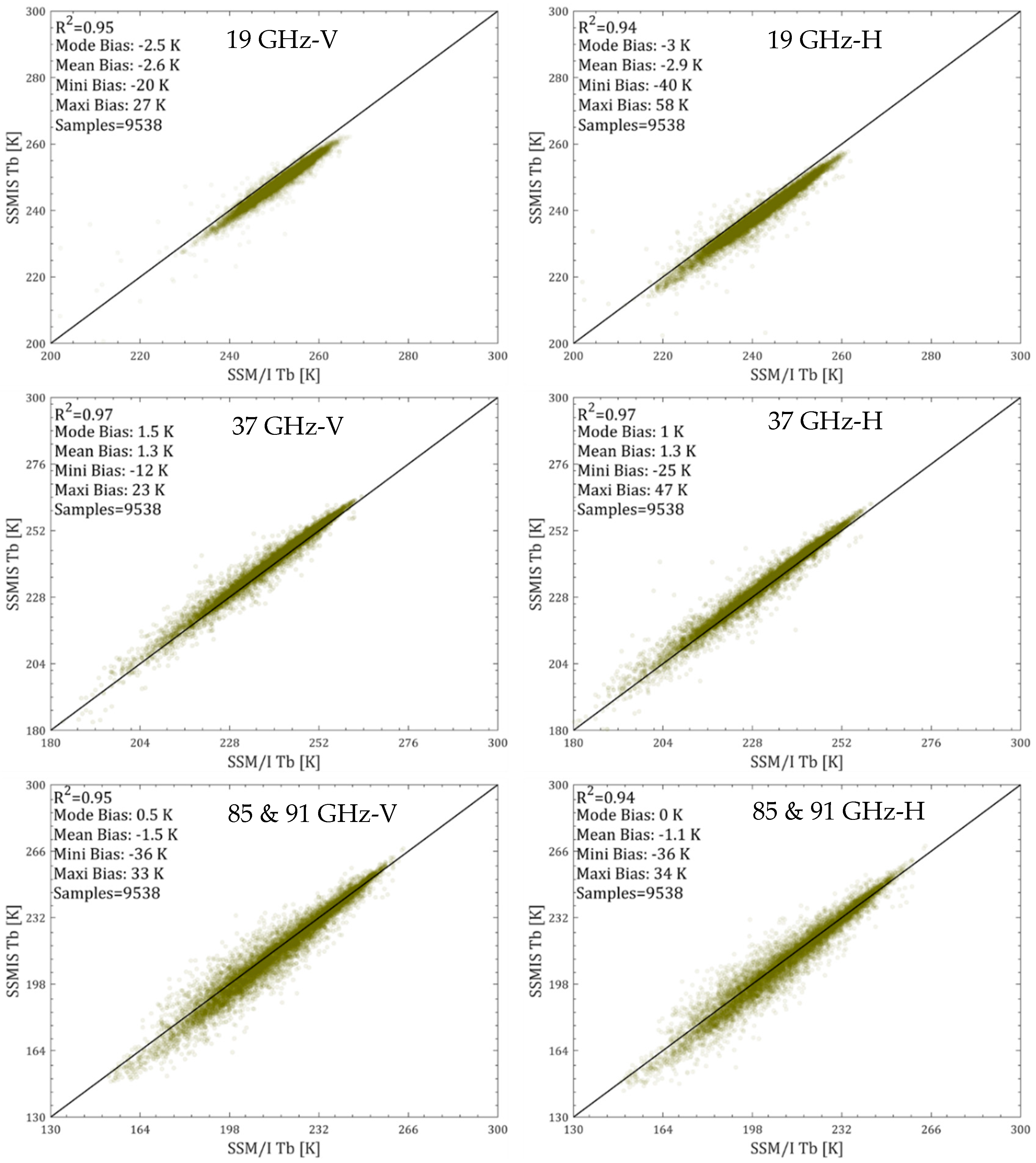
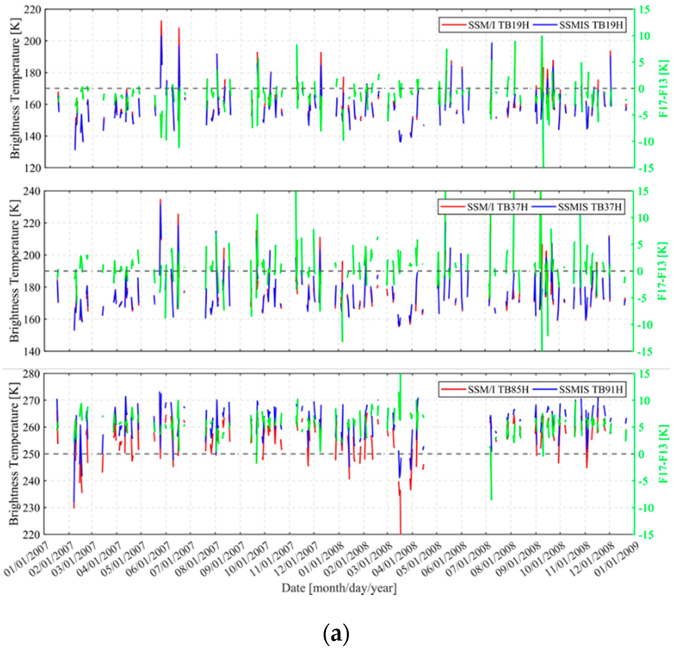
3.1. Comparison between SSM/I and SSMIS Brightness Temperature

To study the consistency of Tb in snow-covered areas, scatter plots of Tbs between SSM/I and SSMIS are shown in Figure 2. In this study, only pixels where ground-measured snow depths are greater than 3 cm are considered as snow cover. There are 9538 pairwise Tb samples in snow-covered areas based on the in situ snow depth and PMW snow cover detection [42]. Here, the representativeness of the weather station was not assessed, and may resulting in some uncertainties in the bias analysis. Results show that the coefficient of determination is very high for three channels, greater than 0.94. For the 19 GHz channel, SSM/I tends to yield a higher Tb than SSMIS. The mode (repeated most often) and mean biases for V and H polarizations are around −3 and −2.5 K, respectively. The 19 GHz channel is more vulnerable to mixed pixels because it has the largest footprint of the three SSM/I frequencies [37]. For the 37 GHz channel, SSMIS tends to yield a higher Tb than SSM/I. The bias is about 1.3 K. This demonstrates that the SSMIS sensor notably yields lower snow depths than SSM/I for the typical dual-channel snow depth estimation algorithm. For high frequency, such as 85 or 91 GHz, most of the points are located near the 1:1 line, with high R2 values (~0.95) and low values of mean bias (−1.1 K and −1.5 K for H and V polarizations) and mode bias (0 K and 0.5 K for H and V polarizations). In snow-covered areas, although 91 GHz is higher than 85 GHz, the measured Tb is low. One reason is the instrument differences between SSM/I and SSMIS. Another one may be because scattering from snowpack is the dominant effect rather than snow surface emission for high frequency [39,45].
A comparison of Tb between SSM/I and SSMIS in barren land, farmland, grassland, and forest is shown in Figure 3. Due to the similar patterns between H and V polarizations, we only display the result of H polarization here. The grids were considered as pure pixels where the land cover fraction was greater than 85% [39]. To illustrate the influence of snow cover on Tb consistency between SSM/I and SSMIS, in this study, these pairwise pixels were separated into two groups, snow cover vs. snow-free. Li’s snow detection method was employed to determine snow or non-snow based on the assessment work in [43].
Figure 3 (left) shows that the Tb from SSMIS at 19 GHz tends to be lower than the SSM/I observation for each land cover type, with a large mean bias (approximately −2.8 K to −4.6 K) and mode bias (approximately −2.5 K to −4 K). In particular, biases in non-snow areas are larger than these in snow-covered areas (red points vs. green points). Moreover, many of the scatter points are located away from the 1:1 line in non-snow areas, leading to large bias difference. For the 37 GHz channel, the bias is very small and makes no big difference for four main land cover types (Figure 3, middle). For 85 or 91 GHz, biases in snow-covered barren areas and farmlands are high, up to −4 K. This is because the higher frequency, 91 GHz, has stronger scattering from snowpack than 85 GHz, resulting in low Tb for the SSMIS sensor compared with SSM/I [45,46].
For forested snow-covered areas, the biases are close to zero due to the influence of the forest canopy, rather than the snowpack [47,48,49]. Thus, for snow-free areas, the SSMIS tends to yield higher Tb than SSM/I because of high emissions at 91 GHz compared with 85 GHz (Figure 3, left bottom). The correlation between SSM/I and SSMIS is low for snow-free areas compared with snow-covered areas in farmlands and forests (Figure 3, second and bottom rows). The SSMIS tends to obtain higher observations than SSM/I when Tb is smaller than 240 K in non-snow farmlands. For snow-covered areas, most of the points are located near the 1:1 line, with a lower absolute value in term of the maximum and minimum bias compared with snow-free areas. Maximum absolute values of biases are 23, 63, and 42 K for 19, 37, and 85 (91) GHz, respectively, while they are 78, 78, and 92 K for snow-free areas (Table 5). Thus, in snowy (winter) seasons, the consistency between SSM/I and SSMIS is better than in non-snowy seasons.
Temporal patterns between SSM/I and SSMIS were compared in three regions of China in Figure 4. There are four pixels (25 km × 25 km) in each region. The land cover types are mainly farmland and forest in Northeast China (NE), grassland in Xinjiang (XJ), and grassland in Qinghai-Tibetan Plateau (QTP). Tb is the mean brightness temperatures of four pixels. Due to the different swath width and missing data, not every day has an overlapping orbit. Results show that the difference between SSM/I and SSMIS is related to frequency, season, location, and land cover types. Firstly, the higher the frequency, the more likely there will be positive bias. Biases at 19 GHz are negative, while they are positive for 85 (91) GHz. Moreover, SSMIS Tb at the 91 GHz channel is higher than SSM/I Tb at 85 GHz, by up to 25 K. The main reason is the channel difference, around 6 GHz (85 vs. 91 GHz). Secondly, the difference in snow winter season is smaller than in the snow-free season for 19 GHz and 37 GHz, such as in parts of January, February, March, April, and May in 2007 and 2008. The land surface is homogeneous when it is covered with snow. Also, the air temperature is low and stable, so the influence on Tb is small. However, on snow-free days, the temperature and soil moisture change quickly, resulting in poor consistency [37,39]. Lastly, the Tb and Tb biases in QTP are smaller and more stable than observations in XJ and NE, except at a high frequency, 85 or 91 GHz. The main reason is that the air temperature creates a slight variation due to the high elevation [13,50,51]. For the 19 GHz channel, the differences mostly range from −2 to +2 K, and from −5 to +5 K in NE. Table 5 also shows that the bias between SSM/I and SSMIS is related to land cover types. In forested areas, the mean bias is around −3.2 to 4.6 K.

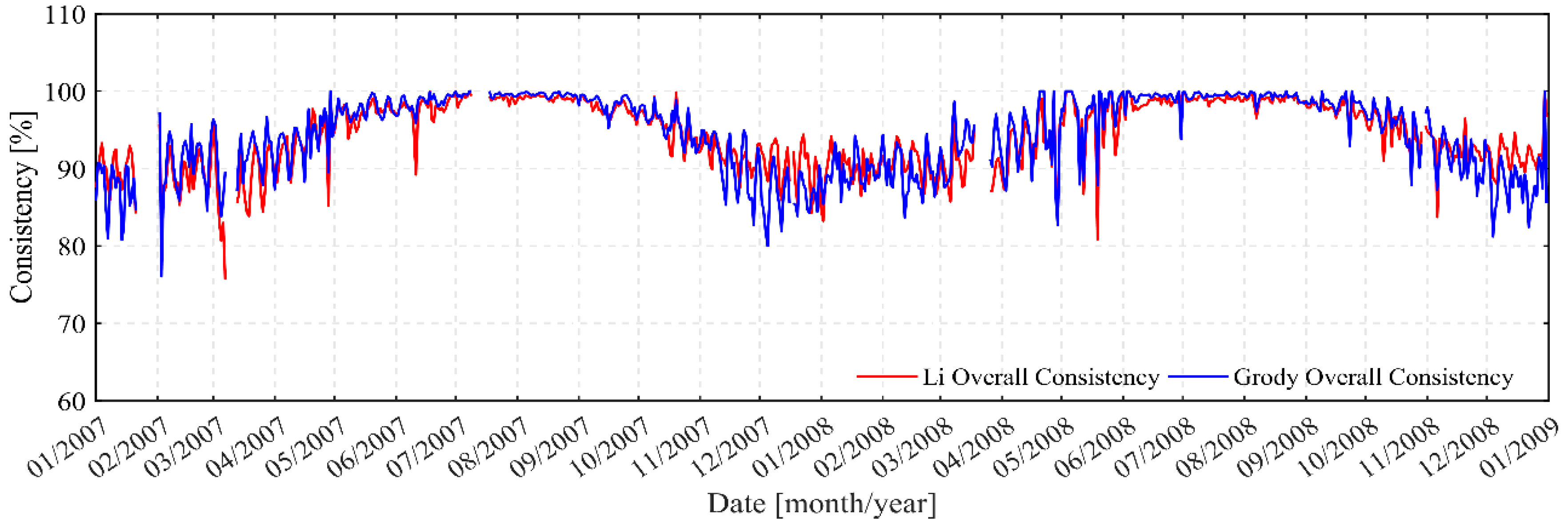
3.2. Comparison between SSM/I and SSMIS Snow Cover Detection

In this paper, the influence of consistency between SSM/I and SSMIS on snow cover detection was studied. Results are shown in Figure 5. Red and blue lines represent the overall consistency between SSM/I and SSMIS for the Li and Grody algorithms, respectively. For any algorithm, the time series patterns are obviously similar. At the beginning of the snow winter seasons, such as November through March of the following year, the consistency is relatively low (minimum, 78%). Namely, for the same snow cover detection algorithm, the result has a big difference (22%) because of the inconsistency in Tb between SSM/I and SSMIS. Based on the number of snow-covered pixels, the difference of snow cover area is up to 25 × 104 km2, an area almost the size of two Hunan provinces. For non-snow seasons, the overall consistency is very high, close to 100%. This is because most satellite pixels are identified as snow-free even though there is a Tb difference between SSM/I and SSMIS. Table 6 shows the overall consistency of snow detection method between SSM/I and SSMIS in winter, spring, summer, and autumn. The consistency is the highest in summer at around 99%. However, in winter, the consistency is poor compared with other seasons, which is related to the snow detection method and the difference between SSM/I and SSMIS. The difference caused by the two sensor platforms leads to opposite snow identification results, snow or snow-free. Thus, the trend analysis for long-term snow cover may be affected by the inconsistency between SSM/I and SSMIS. Table 6 also illustrates that Li’s algorithm has a slight advantage over the Grody method in terms of overall consistency in winter.
Based on the number of snow pixels (25 km × 25 km) identified with the snow cover detection method, the difference in snow cover area between Grody and Li (SCAGrody − SCALi) is shown in Figure 6. Results show that the Grody algorithm tends to yield higher snow cover areas than Li’s. The difference is up to 120 × 104 km2, equaling one-eighth of China’s terrain (~ 960 × 104 km2) and nearly a quarter of stable snow cover (~ 420 × 104 km2) over China. The mean bias in snow winter seasons is between 25 × 104 and 41 × 104 km2. Thus, the snow cover area estimated with the PMW method is not objective and depends on the snow cover detection algorithm. Users who make use of this snow cover product should be cautious.
Dry snow is a type of strong scattering material. Based on the classification criteria shown in Table 3, scattering materials are determined with a positive brightness temperature gradient between low- and high-frequency channels, (Tb19V − Tb37V) or (Tb23V − Tb85V). The comparison of brightness temperature gradient between SSM/I and SSMIS is shown in Figure 7. Classification thresholds are 5 and 0 K for the Grody and Li algorithms, respectively. Purple regions in Figure 7 denote the inconsistency in detection of scattering material between SSM/I and SSMIS for the Grody method. Light blue regions represent the inconsistency for the Li algorithm. Mean biases are −3.9 and −1.7 K for (Tb19V − Tb37V) and (Tb23V − Tb85V), respectively. Namely, the brightness temperature gradient for SSM/I tends to be larger than SSMIS, which results in more scattering materials. Thus, the Tb difference between SSM/I and SSMIS usually leads to different detection results.
Figure 8 shows an example of the spatial distribution of snow cover identified with SSM/I and the corresponding SSMIS detection on 7 January, 18 March, 31 August, and 12 December 2007. For any algorithm, the consistency is very high for 11 August 2007 due to it being snow-free. For the Li algorithm, there is inconsistent detection in the Qinghai Tibet Plateau for 7 January and 12 December 2007 (Figure 8a, yellow circles). Also, there is a big difference between SSM/I and SSMIS for the Grody method (Figure 8b, red and magenta circles). In general, there is poor performance in snowy seasons compared with snow-free seasons in terms of consistency between SSM/I and SSMIS. The snow cover area (Figure 8a, orange and yellow circles) identified by the Li method with SSMIS Tb is larger than the area with SSM/I Tb. For the Grody algorithm, however, SSM/I tends to yield a larger area than SSMIS (Figure 8b, red and magenta circles).

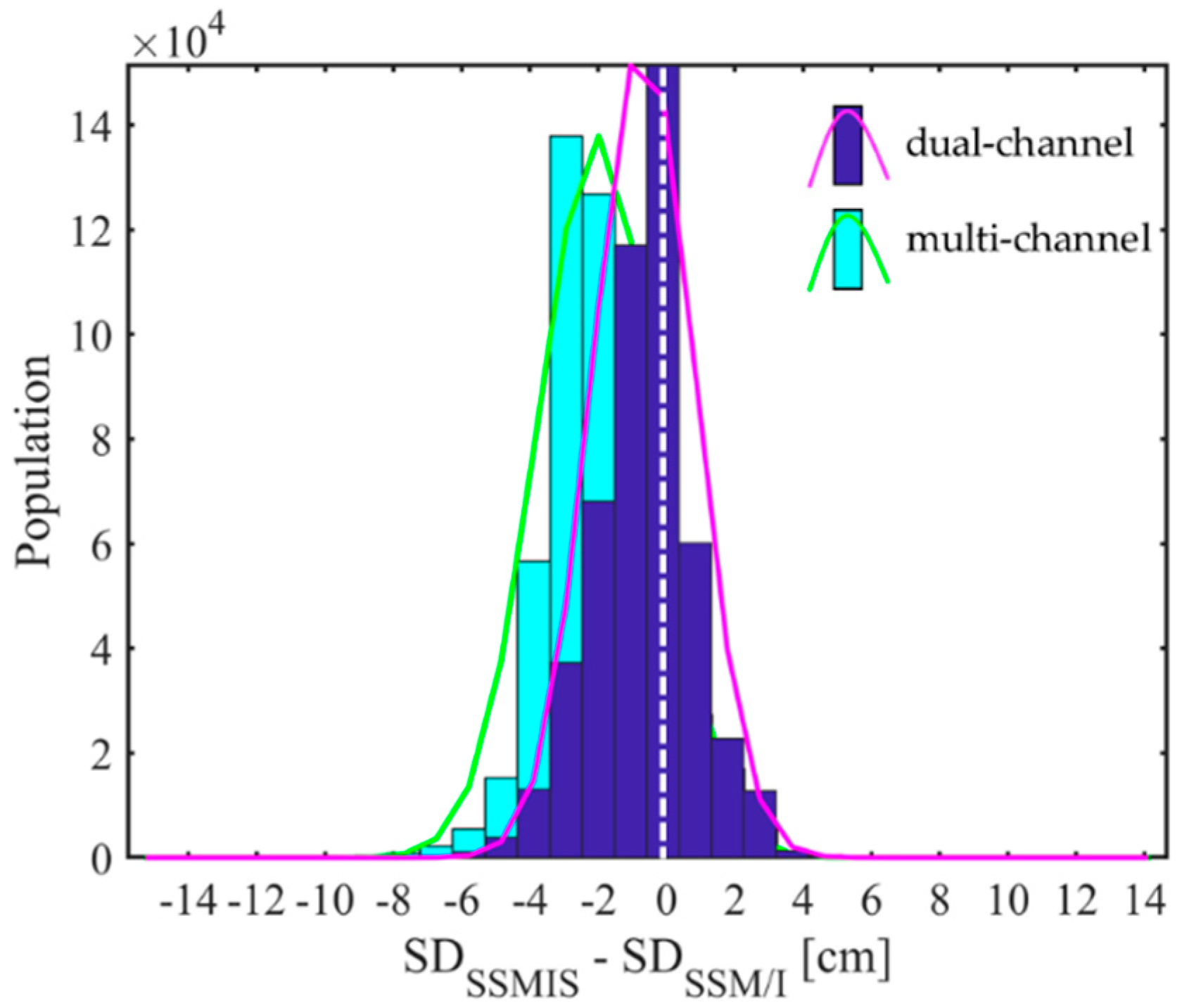
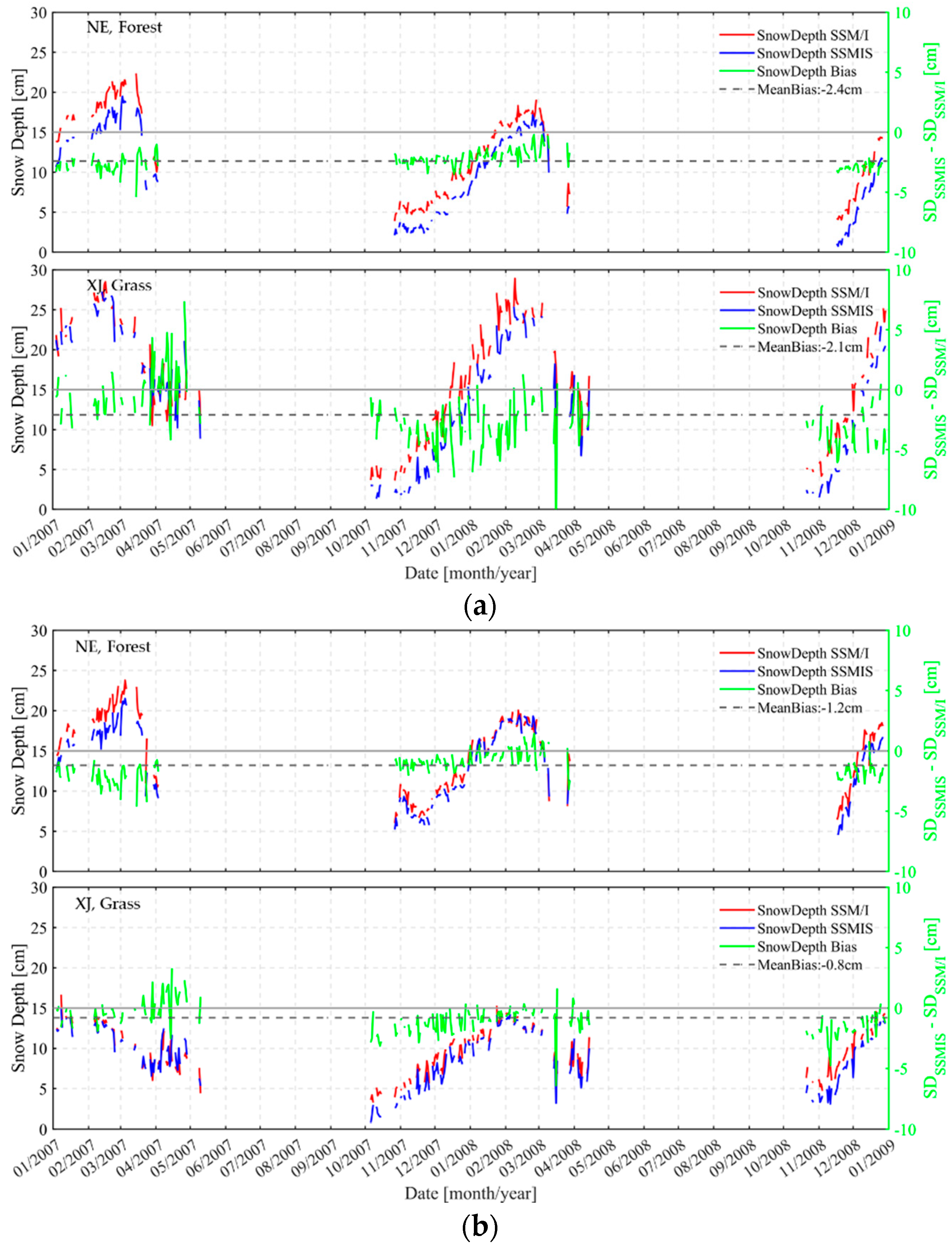
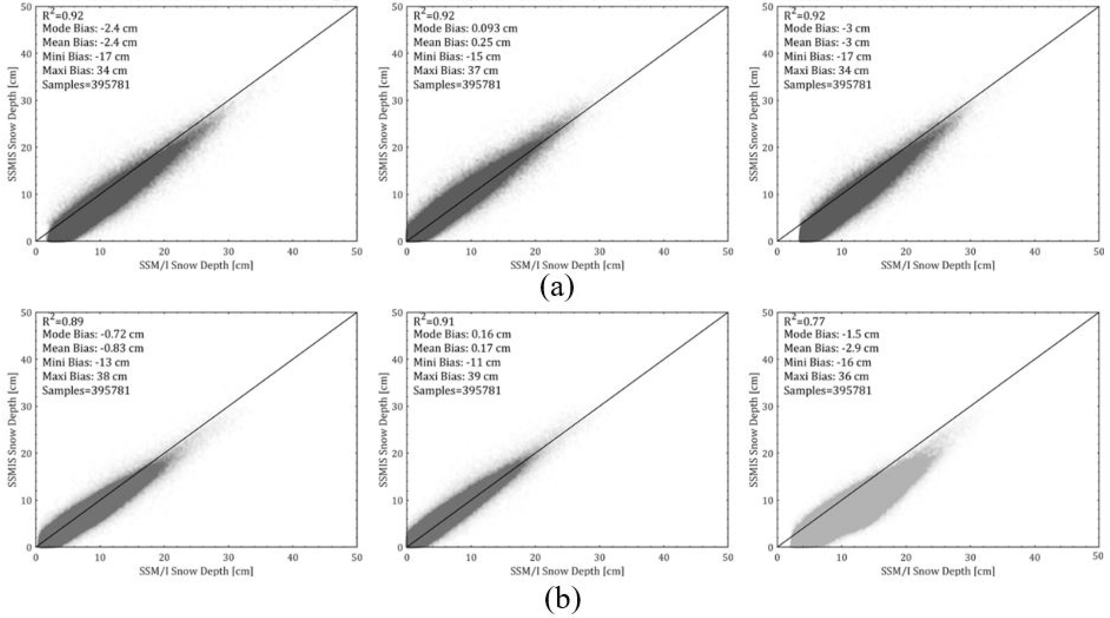
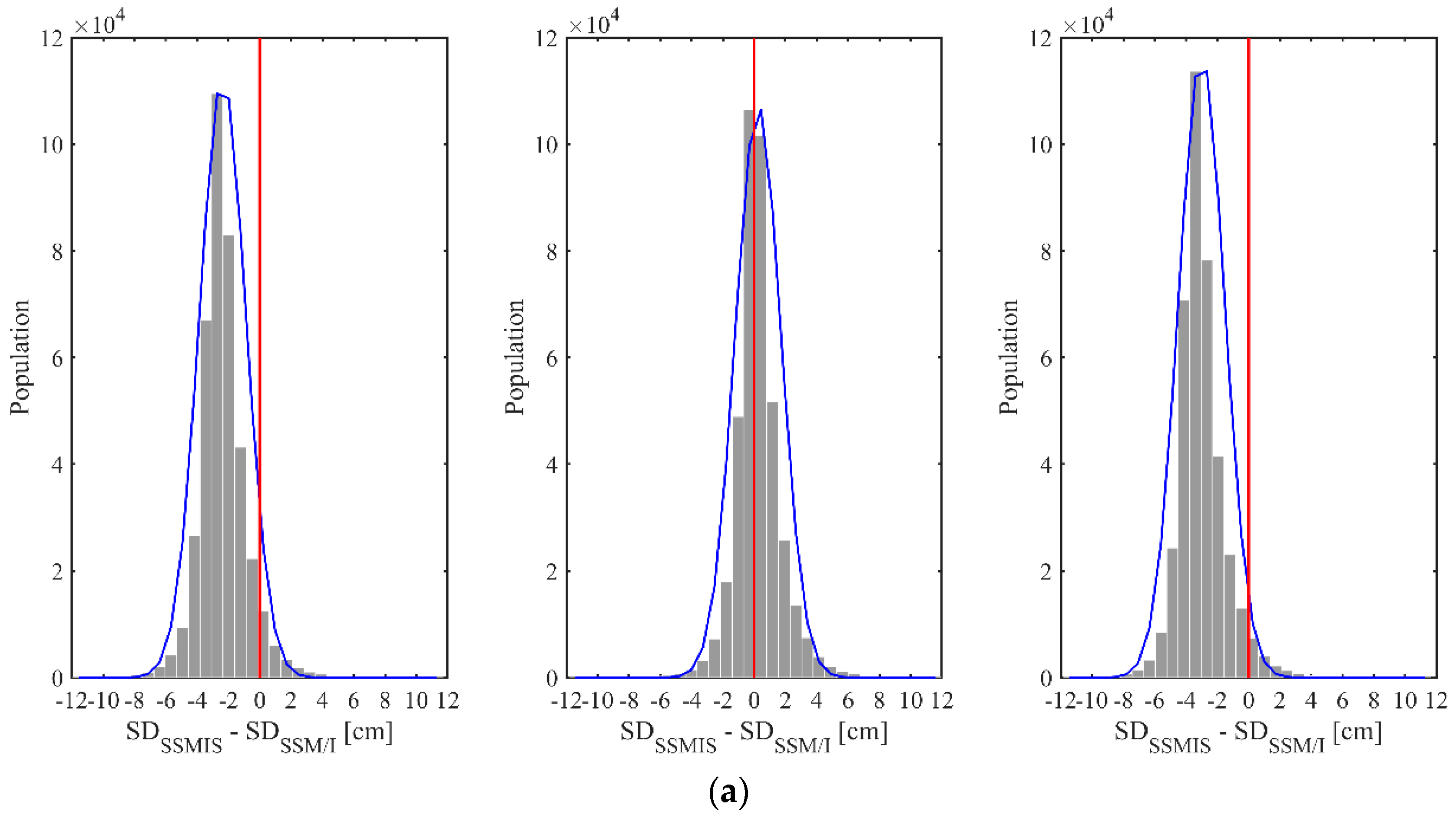
3.3. Comparison between SSM/I and SSMIS Snow Depth

Snow depth was retrieved with the same algorithm but different Tb inputs, SSM/I vs. SSMIS. Scatter plots of snow depth are shown in Figure 9. Results show that the coefficient of determination is very high (R2 = 0.88). However, there are notable snow depth biases between SSM/I and SSMIS for the dual-channel algorithm (Figure 9a). The mode and mean biases are −2.4 and −2.0 cm, respectively. The multichannel method performs better than the dual-channel algorithm with respect to consistency (mode and mean biases: 0 cm and −0.7 cm).
Figure 10 shows a histogram of retrieved snow depth bias between SSM/I and SSMIS, which follows a statistically normal distribution. It is seen that most biases are within ±4 cm for the two histograms. Obviously, the snow depth estimated with SSMIS tends to be lower (mean bias is −2 cm) than that with SSM/I for the dual-channel algorithm. According to the comparison of Tb in Section 3.1, SSMIS tends to yield lower Tb (mean bias, −2.5 to 4.6 K) than SSM/I at 19 GHz. Moreover, SSMIS usually slightly overestimates Tb (mean bias, 1.3 K) compared with SSM/I at 37 GHz. The mean bias is very small (−0.67 cm) for the multichannel method. Figure 10 shows that most biases are between −2 and 2 cm. This better consistency between SSM/I and SSMIS is attributed to the combination of three channels (19, 37, 85, or 91 GHz) for the multichannel method.
Figure 11 shows time series of biases between SSM/I and SSMIS for the dual-channel algorithm and multichannel algorithm, respectively. The satellite pixels selected are the same as the areas in Figure 3. Figure 11a shows that the mean biases in Northeast China and Xinjiang are −2.4 and −2.1 cm, respectively. In addition, time series of biases are stable in Northeast China for the dual-channel algorithm. Comparing the Tb difference in Figure 3a and the snow depth in Figure 11a, the result is consistent with respect to bias. Forest, indeed, attenuates the radiation emitted by the underlying snowpack and emits its own radiation toward the satellite-based radiometer. Therefore, the satellite observation is mainly associated with the emissions from the forest canopy [47,48,49]. However, the satellite observation in Xinjiang is plagued by a number of challenges, including the distinguishing of scattering materials, snow microphysical properties, and liquid water within snowpack. Figure 11a also shows that the bias tends to be bigger at the end of snowy seasons. This is because the presence of liquid water due to the relatively high air temperature in these months makes the retrieval of snow depth impossible [45,52]. Figure 11b shows that the bias between SSM/I and SSMIS for the multichannel algorithm is stable and small (approximately −1 cm). This can be attributed to the canceling effect of the positive and negative values for the multichannel combination. Another factor is that the multichannel algorithm accounts for the influence of mixed pixels on snow depth estimation, leading to small bias [39,53].

4. Discussion

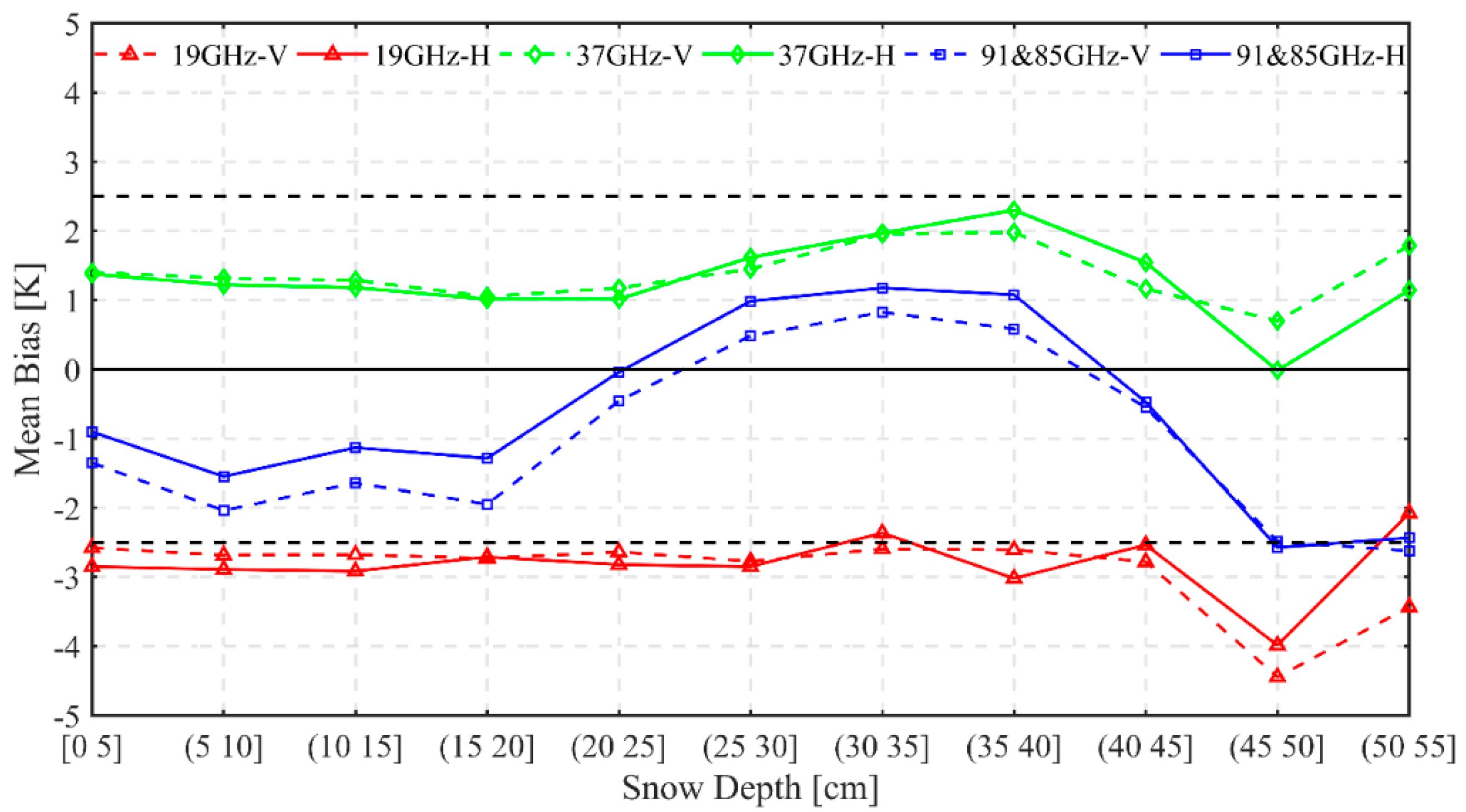
4.1. The Influence of Snow Depth on Brightness Temperature Bias

According to Section 3.1, the consistency between SSM/I and SSMIS is relatively good in snow seasons versus non-snow seasons. Here, we discuss the influence of snow depth on the Tb bias based on the in situ snow depth in 2007–2008. Figure 12 shows that the patterns of mean biases with increasing snow depth are similar and stable for 19 GHz horizontal and vertical polarizations. The Tb from SSMIS is about 3 K below SSM/I observation at 19 GHz. For the 37 GHz channel, the mean biases are also relatively stable with increasing snow depth, mostly between 1 and 2 K. The mean biases show a slightly oscillation in various snow depth ranges, between −2 and 1 K for 85 (91) GHz. The positive biases are caused by the emissions from the surface of the snowpack instead of the scattering effect at the 85 (91) GHz channel [17,39,46]. Interestingly, the brightness temperature difference (Tb37H − Tb85H) tends to be higher for SSMIS than for SSM/I, while (Tb19H − Tb37H) is lower. Therefore, the cancelling effect [(Tb19H − Tb37H)↓+ (Tb37H − Tb85H)↑] occurs for a multichannel algorithm, resulting in better consistency between the SSM/I and SSMIS estimates. These results are in agreement with the work in Section 3.1 and Section 3.3.

4.2. Brightness Temperature Bias in Different Seasons

Time series of biases for observations from SSM/I and SSMIS at horizontal polarization are very similar to those of vertical polarization and, thus, are not shown here. Figure 13 shows that the biases present consistent seasonal oscillation, regardless of mean biases or mode biases. For 19 GHz, the biases are small in winter (DJF) and large in summer (JJA). In general, the absolute values of biases are lower in snow seasons than in snow-free seasons. For a high frequency, such as 37 GHz or 85 (91) GHz, mean biases tend to go from positive to negative values when the seasons change. In snow winter seasons, SSMIS Tb is higher than SSM/I observation, while the trend is the opposite in non-snow seasons. Thus, the bias between SSM/I and SSMIS is related to seasons. Also, especially for 85 (91) GHz, the microwave signal emitted at the surface passes through the atmosphere before being detected by a spaceborne sensor, and is thus subject to the effects of atmospheric absorption and emission [54,55,56]. Moreover, the atmosphere presents obvious seasonal variation, much more complex for the summer than the winter mainly because of the influence of seasonal temperature and incoming solar radiation changes on water vapor [54,57]. Therefore, the bias is the combined result of many factors, including instrument differences, seasons, forest canopy, and atmosphere [34,47,57].

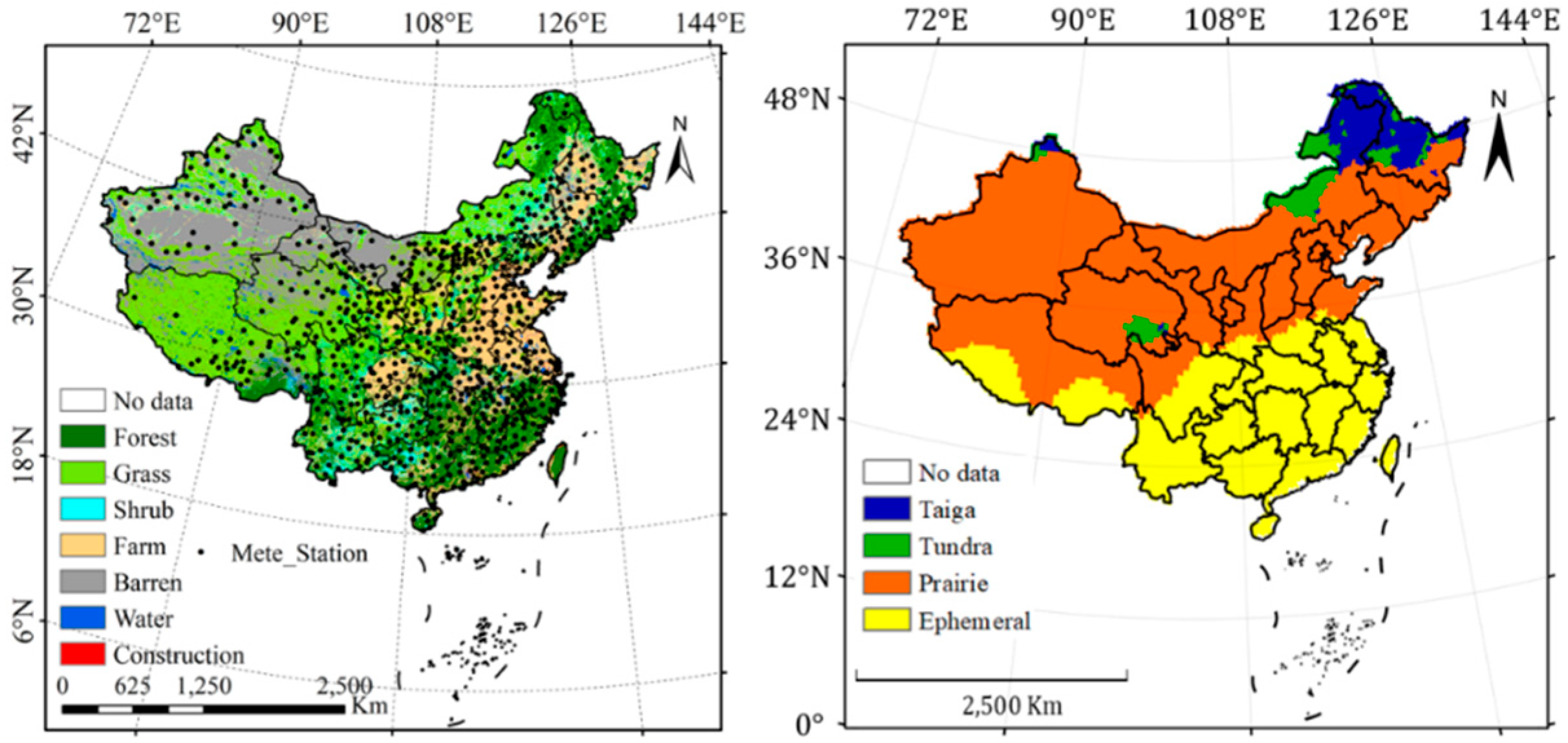
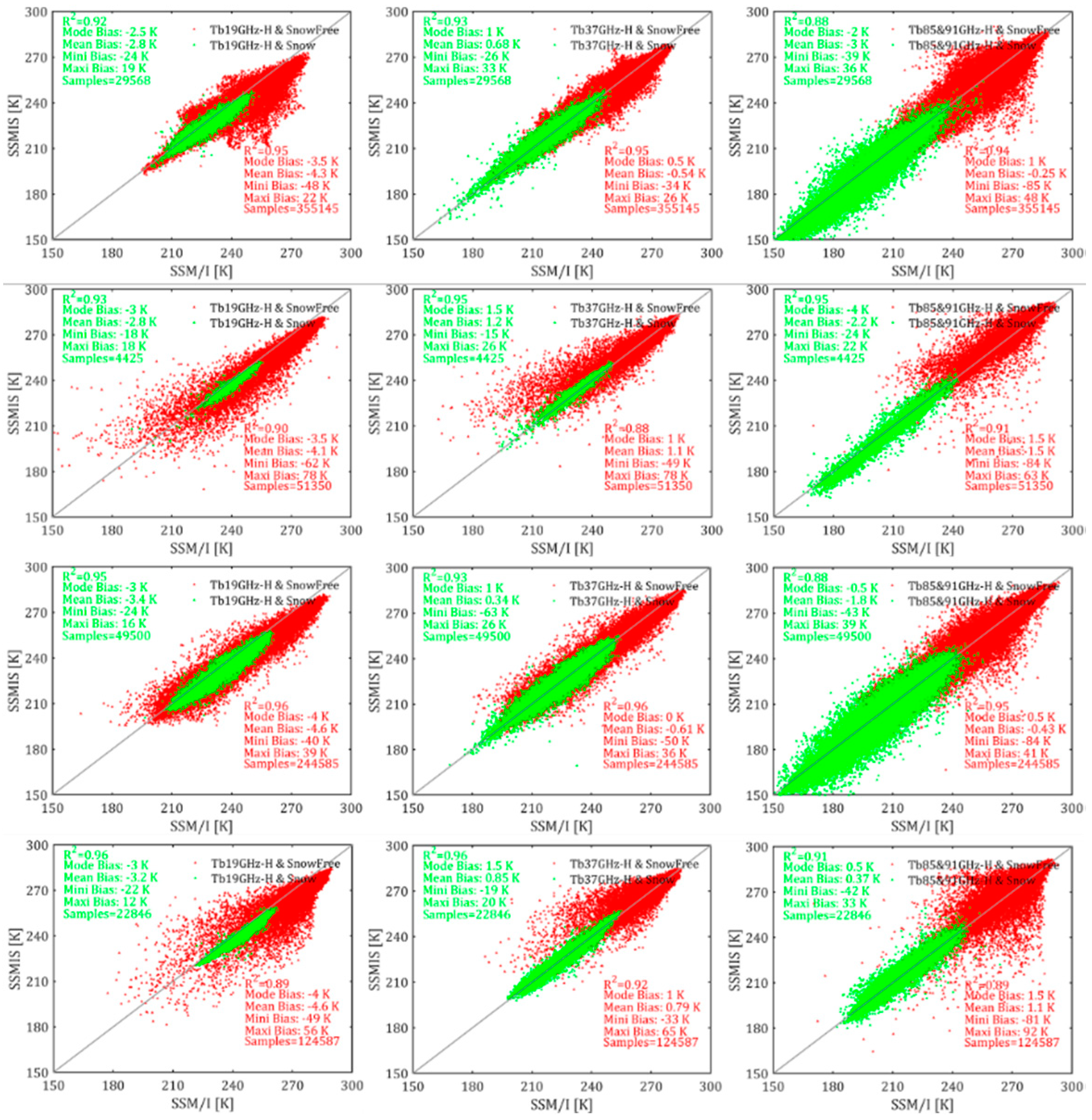
4.3. The Biases in Different Climatological Snow Classes

Although PMW remote sensing has many advantages in monitoring snow cover, accurate retrieval of snow depth or SWE has been challenging due to many factors [5,12,16,45,46,47,48,49]. One of the major challenges is the poor spatial resolution of instruments [58,59]. The variability in snow conditions, land cover, vegetation, and topography in a measured field of view (FOV) may decrease the accuracy of snow parameters retrieved from satellite data [11,12,45,46]. One way of coping with the mixed pixel problem is to take into account the fraction of different land cover types inside a FOV [39,45]. The second focus point is the effect of snow microstructure on its microwave signature. Snow layers have typically distinct grain size, grain type, density, hardness, and wetness, which affects the scattering of microwave radiation from dry snow [5,6,11,12,13]. Even small changes in snow microstructure, such as snow grain, modify the measured Tb notably [60]. In wet snow, the presence of liquid water with a much higher permittivity than that of ice strongly affects the permittivity of the mixture, resulting in higher absorption and poor penetration depth [6]. Therefore, in wet snow conditions, snow depth cannot be retrieved by PMW remote sensing data.
To consider the influence of snow cover characteristics on consistency between SSM/I and SSMIS, we studied the biases in Tb and snow depth estimates in various climatological snow classes based on snow classification system in [40]. Figure 14 shows the time series of Tb biases between SSM/I and SSMIS for four snow climate classes at 19, 37, and 85 (91) GHz channels. For 19 GHz, there is no notable difference in consistency for four snow classes in snow winter seasons (Figure 14a). This could be due to the lower sensitivity to snow cover at low frequency. However, there are clear bias differences among the four classes in non-snow seasons (April to October). The Tb bias for ephemeral snow class is lower than others, and tundra and taiga snow display the largest biases, up to −7 K. The tundra and taiga snow classes are distributed in high latitudes, around 50°N, and biases are most noticeable near the poles (poleward of 60° in latitude) and in mountainous regions [15]. For 37 GHz, there are similar temporal patterns with 19 GHz. In January and December, the biases are relatively low for taiga snow class (Figure 14b). This variability could be related to characteristics of the taiga snow class, low snow and air temperature, small snow density, and stable snow cover [40,45,61]. For 85 (91) GHz, bias time series have irregular temporal patterns except for ephemeral class (Figure 14c).
Figure 15 displays the monthly mean biases and coefficients of determination (R2) of SSM/I and SSMIS estimates for the four snow classes. The correlation between SSM/I and SSMIS snow depths is poor in April, October, and November. This is because of high air temperature and thin snow cover. High temperature tends to result in wet snow and even rainfall. In wet snow conditions, it is impossible to retrieve snow depth with PMW remote sensing. Shallow snow cover usually leads to partially snow-covered pixels due to coarse spatial resolution of satellite data. Thus, these characteristics could result in difficulty in estimating snow depth using Tb from PMW sensors.
For dual-channel algorithm, the biases range from −1.5 to 3 cm for four snow classes (Figure 15, top). Monthly snow depth biases are relatively low for prairie and ephemeral snow classes. This is because snow cover is thin and has no complex layer structure (Table 1). The effect of snow microstructure on satellite signals is clear for tundra and taiga classes. These two classes differ by snow density and depth, typical grain shapes, layer structure, and the number of layers [60]. There are huge metamorphic changes inside the snowpack over the winter [61]. The microstructure mainly defines how microwave radiation is scattered in the snowpack. However, most snow depth retrieval algorithms assumed one homogeneous snow layer, even though snow typically has a very complex layer structure. For the multichannel algorithm, there are similar patterns for taiga snow class, showing high bias between SSM/I and SSMIS (Figure 15, bottom). In the prairie areas, the snow depth estimates are more reliable because vegetation is sparse; thus, there is little extraneous emission [61,62].

4.4. Intercalibration in Different Sensors

It is worth noting that there are notable Tb differences due to different calibration procedures, interpolation methods, and sensor specifications between SSM/I and SSMIS, resulting in inconsistency in snow cover area and snow depth for long-term records. SSMIS EASE-Grid Tb fields are gridded using an inverse distance squared method instead of the Backus-Gilbert interpolation, which had been used for the earlier sensors [15]. Since the two interpolation methods differ, there is a difference in the Tb fields. Thus, the intercalibration of two sensors is required so that their observations can maintain high consistency. In this study, calibration equations based on linear regression in Section 3.1 were used, as shown in Table 7. To illustrate the influence of snow cover on the consistency between SSM/I and SSMIS, two groups calibration equations were compared. Group 1 is from linear fitting of pairwise Tbs in snow cover areas. Group 2 is also statistical regression but regardless of whether there is snow cover or not. Based on the equations in Table 7, the Tbs at all channels from SSM/I (F13) are calibrated. Here, calibrated Tbs with the two groups’ equations are recorded as F13CS (calibrated with group 1) and F13CA (calibrated with group 2), respectively.
Scatter plots of snow depths (F17 vs. F13; F17 vs. F13CS; F17 vs. F13CA) are compared in Figure 16. Results show that the intercalibration only in snow cover areas performs well against that of all areas together. Figure 16a shows that correlation coefficients undergo no change and are always 0.92 for the dual-channel algorithm. Mean biases change from −2.4 to 0.25, improving the consistency in snow depth after calibration for SSM/I in snow cover areas (Figure 16a, left vs. middle). However, the consistency changes for the worse when SSM/I Tb is calibrated with group 2 equations (Figure 16a, right). For the multichannel algorithm, correlation coefficients are improved from 0.89 to 0.91 after calibration with group 1 equations (Figure 16b, left vs. middle). Mean biases and mode biases are closer to zero than those without calibration. What is surprising is that after calibration to SSM/I with the group 2 equations, the relationship becomes distorted and worse (Figure 16b, right). Moreover, the correlation coefficient is as low as 0.77. Figure 17 shows histograms of snow depth biases between SSM/I and SSMIS. It is seen that most biases are within ±2 cm for the two algorithms after the intercalibration of two sensors in snow cover areas. Obviously, biases mainly span from −6 to 0 cm for the dual-channel algorithm (Figure 17a, left) after calibration with group 2 equations, and even worse for multichannel algorithm, from −8 to 2 cm (Figure 17b, left). Table 7 also shows that calibration equations show a big difference between group 1 and 2. Thus, it is better to conduct intercalibration based on a specific study.

5. Conclusions

In this study, we evaluated the consistency in satellite Tb, snow cover detection, and snow depth estimation from different generations of sensors (SSM/I vs. SSMIS) that had temporal and spatial overlap. Results demonstrate that although the SSM/I and SSMIS sensors are similar, there are still differences in terms of the observed Tbs caused by their different calibration procedures, interpolation methods, and sensor specifications. Fortunately, the biases between SSM/I and SSMIS are related to seasons, with relatively good consistency in snow winter seasons against non-snow seasons. For 19 GHz, the biases in snow winter seasons span from −2 to −3 K and from −4 to −5 K for non-snow seasons. There is a slight Tb bias between SSM/I and SSMIS at 37 GHz regardless of the season, ranging from −2 to 2 K. Interestingly, there are notable mean biases for 85 (91) GHz in snow seasons of as high as −3 K. This is related to channel difference (~6 K) and the absorption and emission effects.
The consistency in the snow cover detection between SSM/I and SSMIS was evaluated for the Grody algorithm and the Li method. The results showed that the overall consistency is between 80% and 100% for any snow cover detection algorithm. In snow winter seasons, the consistency is relatively low, spanning from 80% to 90%. Namely, there are 10%-20% differences between SSM/I and SSMIS for the same snow cover detection algorithm. Based on snow-covered satellite pixels, the difference of snow cover area is between 12.5 × 10⁴ and 25 × 104 km2. Moreover, the most intractable problem is that there are huge differences in snow cover area between the Grody algorithm and the Li method. The difference is as high as 120 × 104 km2, equaling one-eighth of China or nearly a quarter of the stable snow cover over China. Thus, although snow cover detection is necessary for snow depth estimation, the snow cover area based on the PMW method is not objective or reliable.
The influence of Tb consistency between SSM/I and SSMIS on snow depth estimation was analyzed. Results show that the mean biases are −2 cm and −0.67 cm for dual-channel and multichannel algorithms, respectively. The multichannel algorithm performs well against the dual-channel algorithm in terms of consistency. This is mainly attributed to the cancelling effect of multichannel combination. For the dual-channel method (Tb19H − Tb37H), however, underestimation of SSMIS-estimated snow depth relative to SSM/I is inevitable due to the Tb bias. In this study, we evaluated consistencies in four seasonal snow classes. Results show that there are notable bias differences between SSM/I- and SSMIS-estimated snow depths in the tundra and taiga snow classes based on time series comparisons. Here, we note that several aspects of influencing snow depth biases include instrument differences, sensor calibration uncertainties, and snow cover characteristics in various snow classes.
A few studies on the intercalibration of the two sensors were performed and demonstrated that the consistency was high after calibration. Our results denote that the time series of biases show seasonal oscillation. Thus, our conclusion is that the inter-sensor calibration purely in snow winter seasons is more reasonable in terms of snow study, rather than calibration together with snow and non-snow seasons. In the same season, the trend of systematic biases is similar and consistent, which makes intercalibration easier and more effective. To maximize the use of satellite data for long-term monitoring, in this study, huge effort was focused on the consistency of SSM/I and SSMIS and the influence of Tb bias on snow depth estimation and snow cover detection. However, the error caused by inconsistency in Tb is minor as compared to the algorithm uncertainties. Thus, it is most important to improve the snow depth retrieval algorithms. Future research on this topic will validate snow depth estimates from SSM/I and SSMIS using ground truth observations.

Author Contributions

Conceptualization, L.J. and J.Y.; Methodology, L.J.; Software Validation, Formal Analysis and Investigation, J.Y., L.D., J.P., S.W. and G. W; Writing-Original Draft Preparation, Writing-Review & Editing, and Visualization, J.Y., L.J., L.D. and J.P.; Data Curation, J.Y.; Project Administration, L.J.; Funding Acquisition and Resources, L.J.

Funding

This research was funded by the Science and Technology Basic Resources Investigation Program of China [2017FY100502] and the National Natural Science Foundation of China [41671334].

Acknowledgments

The authors would like to thank the China Meteorological Administration, National Geomatics Center of China, and National Snow and Ice Data Center for providing land cover products and satellite data.

Conflicts of Interest

The authors declare no conflict of interest.

References

  1. Bormann, J.; Brown, R.; Derksen, C.; Painter, H. Estimating snow-cover trends from space. Nat. Clim. Chang. 2018, 8, 924–928. [Google Scholar] [CrossRef]
  2. Derksen, C.; Brown, R. Spring snow cover extent reductions in the 2008–2012 period exceeding climate model projections. Geophys. Res. Lett. 2012, 39, 1–6. [Google Scholar] [CrossRef]
  3. Fernandes, R.; Zhao, H.; Wang, X.; Key, J.; Qu, X.; Hall, A. Controls on Northern Hemisphere snow albedo feedback quantified using satellite Earth observations. Geophys. Res. Lett. 2009, 36, 1–6. [Google Scholar] [CrossRef]
  4. Hernández-Henríquez, M.; Déry, S.; Derksen, C. Polar amplification and elevation-dependence in trends of Northern Hemisphere snow cover extent, 1971–2014. Environ. Res. Lett. 2015, 10, 044010. [Google Scholar] [CrossRef]
  5. Takala, M.; Ikonen, J.; Luojus, K.; Lemmetyinen, J.; Metsamaki, S.; Cohen, J.; Nadir, A.; Pulliainen, J. New Snow Water Equivalent Processing System with Improved Resolution Over Europe and its Applications in Hydrology. IEEE J. Sel. Top. Appl. Earth Obs. Remote Sens. 2017, 10, 428–436. [Google Scholar] [CrossRef]
  6. Lemmetyinen, J.; Schwank, M.; Rautiainen, K.; Kontu, A.; Parkkinen, T.; Mätzler, C.; Wiesmann, A.; Wegmüller, U.; Derksen, C.; Toose, P.; et al. Snow density and ground permittivity retrieved from L-band radiometry: Application to experimental data. Remote Sens. Environ. 2016, 180, 377–391. [Google Scholar] [CrossRef]
  7. Safavi, H.; Sajjadi, S.; Raghibi, V. Assessment of climate change impacts on climate variables using probabilistic ensemble modeling and trend analysis. Theor. Appl. Climatol. 2017, 130, 635–653. [Google Scholar] [CrossRef]
  8. De Rosnay, P.; Balsamo, G.; Albergel, C.; Muñoz-Sabater, J.; Isaksen, L. Initialisation of land surface variables for numerical weather prediction. Surv. Geophys. 2014, 35, 607–621. [Google Scholar] [CrossRef]
  9. Bell, V.; Kay, A.; Davies, H.; Jones, R. An assessment of the possible impacts of climate change on snow and peak river flows across Britain. Clim. Chang. 2016, 136, 539–553. [Google Scholar] [CrossRef] [Green Version]
  10. Barnett, T.P.; Adam, J.; Lettenmaier, D. Potential impacts of a warming climate on water availability in snow-dominated regions. Nature 2005, 438, 303–309. [Google Scholar] [CrossRef] [PubMed]
  11. Takala, M.; Luojus, K.; Pulliainen, J.; Derksen, C.; Lemmetyinen, J.; Kärnä, J.-P.; Koskinen, J.; Bojkov, B. Estimating northern hemisphere snow water equivalent for climate research through assimilation of space-borne radiometer data and ground-based measurements. Remote Sens. Environ. 2011, 115, 3517–3529. [Google Scholar] [CrossRef]
  12. Che, T.; Dai, L.; Zheng, X.; Li, X.; Zhao, K. Estimation of snow depth from passive microwave brightness temperature data in forest regions of northeast China. Remote Sens. Environ. 2016, 183, 334–349. [Google Scholar] [CrossRef]
  13. Dai, L.; Che, T.; Ding, Y.; Hao, X. Evaluation of snow cover and snow depth on the Qinghai–Tibetan Plateau derived from passive microwave remote sensing. Cryosphere 2017, 11, 1933–1948. [Google Scholar] [CrossRef]
  14. Luojus, K.; Pullianinen, J.; Takala, M.; Lemmetyinen, J.; Kangwa, M.; Smolander, T.; Derksen, C.; Pinnock, S. ESA Globsnow: Algorithm Theoretical Basis Document-SWE-algorithm. Technical Report, European Space Agency (ESA). 2013. Available online: http://cedadocs.ceda.ac.uk/id/eprint/1263 (accessed on 13 May 2019).
  15. Armstrong, R.; Knowles, K.; Brodzik, M.; Hardman, M. DMSP SSM/I-SSMIS Pathfinder Daily EASE-Grid Brightness Temperatures, Version 2; NASA National Snow and Ice Data Center Distributed Active Archive Center: Boulder, CO, USA, 1994. [Google Scholar] [CrossRef]
  16. Berg, W.; Kroodsma, R.; Kummerow, C.D.; McKague, D.S. Fundamental Climate Data Records of Microwave Brightness Temperatures. Remote Sens. 2018, 10, 1306. [Google Scholar] [CrossRef]
  17. Kelly, R. The AMSR-E snow depth algorithm: Description and initial results. J. Remote Sens. Soc. Jpn. 2009, 29, 307–317. [Google Scholar] [CrossRef]
  18. Knowles, K.; Njoku, E.; Armstrong, R.; Brodzik, M. Nimbus-7 SMMR Pathfinder Daily EASE-Grid Brightness Temperatures, Version 1; NASA National Snow and Ice Data Center Distributed Active Archive Center: Boulder, CO, USA, 2000. [Google Scholar] [CrossRef]
  19. Kawanishi, T.; Sezai, T.; Ito, Y.; Imaoka, K.; Takeshima, T.; Ishido, Y.; Shibata, A.; Miura, M.; Inahata, H.; Spencer, R. The Advanced Scanning Microwave Radiometer for the Earth Observing System (AMSR-E): NASDA’s contribution to the EOS for global energy and water cycle studies. IEEE Trans. Geosci. Remote Sens. 2003, 41, 184–194. [Google Scholar] [CrossRef]
  20. Imaoka, K.; Takashi, M.; Misako, K.; Marehito, K.; Norimasa, I.; Keizo, N. Status of AMSR2 instrument on GCOM-W1, earth observing missions and sensors: Development, implementation, and characterization II. Proc. SPIE 2012, 8528, 852815. [Google Scholar] [CrossRef]
  21. Yang, H.; Weng, F.; Lv, L.; Lu, N.; Liu, G.; Bai, M.; Qian, Q.; He, J.; Xu, H. The FengYun-3 microwave radiation imager on-orbit verification. IEEE Trans. Geosci. Remote Sens. 2011, 49, 4552–4560. [Google Scholar] [CrossRef]
  22. Pulliainen, J.; Grandell, J.; Hallikainen, M. HUT snow emission model and its applicability to snow water equivalent retrieval. IEEE Trans. Geosci. Remote Sens. 1999, 37, 1378–1390. [Google Scholar] [CrossRef]
  23. Pulliainen, J. Mapping of snow water equivalent and snow depth in boreal and sub-arctic zones by assimilating space-borne microwave radiometer data and ground-based observations. Remote Sens. Environ. 2006, 101, 257–269. [Google Scholar] [CrossRef]
  24. Dai, L.; Che, T.; Ding, Y. Inter-Calibrating SMMR, SSM/I and SSMI/S Data to Improve the Consistency of Snow-Depth Products in China. Remote Sens. 2015, 7, 7212–7230. [Google Scholar] [CrossRef] [Green Version]
  25. Che, T.; Li, X.; Jin, R.; Armstrong, R.; Zhang, T. Snow depth derived from passive microwave remote-sensing data in China. Ann. Glaciol. 2008, 49, 145–154. [Google Scholar] [CrossRef] [Green Version]
  26. Dai, L.; Che, T.; Wang, J.; Zhang, P. Snow depth and snow water equivalent estimation from AMSR-E data based on a priori snow characteristics in Xinjiang, China. Remote Sens. Environ. 2012, 127, 14–29. [Google Scholar] [CrossRef]
  27. Larue, F.; Royer, A.; DeSève, D.; Langlois, A.; Roy, A.; Brucker, L. Validation of GlobSnow-2 snow water equivalent over Eastern Canada. Remote Sens. Environ. 2017, 194, 264–277. [Google Scholar] [CrossRef] [Green Version]
  28. Pulliainen, J.; Aurela, M.; Laurila, T.; Aalto, T.; Takala, M.; Salminen, M.; Kulmala, M.; Barr, A.; Heimann, M.; Lindroth, A. Early snowmelt significantly enhances boreal springtime carbon uptake. Proc. Natl. Acad. Sci. USA 2017, 114, 11081–11086. [Google Scholar] [CrossRef] [PubMed] [Green Version]
  29. Chander, G.; Hewison, T.; Fox, N.; Wu, X.; Xiong, X.; Blackwell, W. Overview of Intercalibration of Satellite Instruments. IEEE Trans. Geosci. Remote Sens. 2013, 51, 1056–1080. [Google Scholar] [CrossRef]
  30. Derksen, C.; Walker, A. Identification of systematic bias in the cross-platform (SMMR and SSM/I) EASE-grid brightness temperature time series. IEEE Trans. Geosci. Remote Sens. 2003, 41, 910–915. [Google Scholar] [CrossRef]
  31. Cavalieri, D.; Parkinson, C.; DiGirolamo, N.; Ivanoff, A. Intersensor Calibration Between F13 SSMI and F17 SSMIS for Global Sea Ice Data Records. IEEE Geosci. Remote Sens. Lett. 2012, 9, 233–236. [Google Scholar] [CrossRef]
  32. Okuyama, A.; Imaoka, K. Intercalibration of Advanced Microwave Scanning Radiometer-2 (AMSR2) Brightness Temperature. IEEE Trans. Geosci. Remote Sens. 2015, 53, 4568–4577. [Google Scholar] [CrossRef]
  33. Meier, W.; Khalsa, S.; Savoie, M. Intersensor calibration between F-13 SSM/I and F-17 SSMIS near-real-time sea ice estimates. IEEE Trans. Geosci. Remote Sens. 2011, 49, 3343–3349. [Google Scholar] [CrossRef]
  34. Cho, E.; Tuttle, S.E.; Jacobs, J.M. Evaluating Consistency of Snow Water Equivalent Retrievals from Passive Microwave Sensors over the North Central U. S.: SSM/I vs. SSMIS and AMSR-E vs. AMSR2. Remote Sens. 2017, 9, 465. [Google Scholar] [CrossRef]
  35. Yan, B.; Weng, F.; Okamoto, K. Improved estimation of snow emissivity from 5 to 200 GHz. In Proceedings of the 8th Specialist Meeting on Microwave Radiometry and Remote Sensing Applications, Rome, Italy, 24–27 February 2004. [Google Scholar]
  36. Yan, B.; Weng, F. Intercalibration Between Special Sensor Microwave Imager/Sounder and Special Sensor Microwave Imager. IEEE Trans. Geosci. Remote Sens. 2008, 46, 4. [Google Scholar] [CrossRef]
  37. Cao, C.; Weinreb, M.; Xu, H. Predicting simultaneous nadir overpasses among polar-orbiting meteorological satellites for the intersatellite calibration of radiometers. J. Atmos. Ocean. Technol. 2004, 21, 537–542. [Google Scholar] [CrossRef]
  38. Du, J.; Kimball, J.S.; Shi, J.; Jones, L.A.; Wu, S.; Sun, R.; Yang, H. Inter-Calibration of Satellite Passive Microwave Land Observations from AMSR-E and AMSR2 Using Overlapping FY3B-MWRI Sensor Measurements. Remote Sens. 2014, 6, 8594–8616. [Google Scholar] [CrossRef] [Green Version]
  39. Jiang, L.; Wang, P.; Zhang, L.; Yang, H.; Yang, J. Improvement of snow depth retrieval for FY3B-MWRI in China. Sci. China Earth Sci. 2014, 44, 531–547. [Google Scholar] [CrossRef]
  40. Sturm, M.; Holmgren, J.; Liston, G.E. A seasonal snow cover classification system for local to global applications. J. Clim. 1995, 8, 1261–1283. [Google Scholar] [CrossRef]
  41. Grody, N.; Basist, A. Global identification of snowcover using SSM/I measurements. IEEE Trans. Geosci. Remote Sens. 1996, 34, 237–249. [Google Scholar] [CrossRef]
  42. Li, X.; Liu, Y.; Zhu, X.; Zheng, Z.; Chen, A. Snow Cover Identification with SSM/I Data in China. J. Appl. Meteorol. Sci. 2007, 18, 12–20. [Google Scholar]
  43. Liu, X.; Jiang, L.; Wu, S.; Hao, S.; Wang, G.; Yang, J. Assessment of Methods for Passive Microwave Snow Cover Mapping Using FY-3C/MWRI Data in China. Remote Sens. 2018, 10, 524. [Google Scholar] [CrossRef]
  44. Yang, J.; Jiang, L.; Wu, S.; Liu, X.; Wang, G.; Hao, S.; Wang, J. Improvement of Snow Depth Estimation Using SSM/I Brightness Temperature in China. In Proceedings of the IGARSS 2018—2018 IEEE International Geoscience and Remote Sensing Symposium, Valencia, Spain, 22–27 July 2018; pp. 5089–5092. [Google Scholar] [CrossRef]
  45. Derksen, C.; Toose, P.; Rees, A.; Wang, L.; English, M.; Walker, A.; Sturm, M. Development of a tundra-specific snow water equivalent retrieval algorithm for satellite passive microwave data. Remote Sens. Environ. 2010, 114, 1699–1709. [Google Scholar] [CrossRef]
  46. Jiang, L.; Shi, J.; Tjuatja, S. Estimation of Snow Water Equivalence Using the Polarimetric Scanning Radiometer From the Cold Land Processes Experiments (CLPX03). IEEE Geosci. Remote Sens. Lett. 2011, 8, 359–363. [Google Scholar] [CrossRef]
  47. Cai, S.; Li, D.; Durand, M.; Margulis, S.A. Examination of the impacts of vegetation on the correlation between snow water equivalent and passive microwave brightness temperature. Remote Sens. Environ. 2017, 193, 244–256. [Google Scholar] [CrossRef]
  48. Li, Q.; Kelly, R. Correcting Satellite Passive Microwave Brightness Temperatures in Forested Landscapes Using Satellite Visible Reflectance Estimates of Forest Transmissivity. IEEE J. Sel. Top. Appl. Earth Obs. Remote Sens. 2017, 10, 3874–3883. [Google Scholar] [CrossRef]
  49. Li, Q.; Kelly, R.; Leppanen, L.; Juho, V.; Kontu, A.; Lemmetyinen, J.; Pulliainen, J. The Influence of Thermal Properties and Canopy-Intercepted Snow on Passive Microwave Transmissivity of a Scots Pine. IEEE Trans. Geosci. Remote Sens. 2019, 99, 1–10. [Google Scholar] [CrossRef]
  50. Dahe, Q.; Shiyin, L.; Peiji, L. Snow cover distribution, variability, and response to climate change in western China. J. Clim. 2006, 19, 1820–1833. [Google Scholar] [CrossRef]
  51. Yang, J.; Jiang, L.; Ménard, C.B.; Luojus, K.; Lemmetyinen, J.; Pulliainen, J. Evaluation of snow products over the Tibetan Plateau. Hydrol. Process. 2015, 29, 3247–3260. [Google Scholar] [CrossRef]
  52. Tedesco, M.; Jeyaratnam, J. A New Operational Snow Retrieval Algorithm Applied to Historical AMSR-E Brightness Temperatures. Remote Sens. 2016, 8, 1037. [Google Scholar] [CrossRef]
  53. Yang, J.; Jiang, L.; Wu, S.; Wang, G.; Wang, J.; Liu, X. Development of a Snow Depth Estimation Algorithm over China for the FY-3D/MWRI. Remote Sens. 2019, 11, 977. [Google Scholar] [CrossRef]
  54. Shi, L.; Qiu, Y.; Shi, J.; Lemmetyinen, J.; Zhao, S. Estimation of Microwave Atmospheric Transmittance Over China. IEEE Geosci. Remote Sens. Lett. 2017, 99, 1–5. [Google Scholar] [CrossRef]
  55. Ji, D.; Shi, J. Water Vapor Retrieval Over Cloud Cover Area on Land Using AMSR-E and MODIS. IEEE J. Sel. Top. Appl. Earth Obs. Remote Sens. 2014, 7, 3105–3116. [Google Scholar] [CrossRef]
  56. Xue, Y.; Forman, B. Atmospheric and Forest Decoupling of Passive Microwave Brightness Temperature Observations Over Snow-Covered Terrain in North America. IEEE J. Sel. Top. Appl. Earth Obs. Remote Sens. 2016, 99, 1–18. [Google Scholar] [CrossRef]
  57. Du, J.; Kimball, J.; Jones, L. Satellite Microwave Retrieval of Total Precipitable Water Vapor and Surface Air Temperature Over Land from AMSR2. IEEE Trans. Geosci. Remote Sens. 2015, 53, 2520–2531. [Google Scholar] [CrossRef]
  58. Gu, L.; Zhao, K.; Huang, B. Microwave Unmixing With Video Segmentation for Inferring Broadleaf and Needleleaf Brightness Temperatures and Abundances from Mixed Forest Observations. IEEE Trans. Geosci. Remote Sens. 2016, 54, 279–286. [Google Scholar] [CrossRef]
  59. Liu, X.; Jiang, L.; Wang, G.; Hao, S.; Chen, Z. Using a Linear Unmixing Method to Improve Passive Microwave Snow Depth Retrievals. IEEE J. Sel. Top. Appl. Earth Obs. Remote Sens. 2018, 11, 4414–4429. [Google Scholar] [CrossRef]
  60. Leppänen, L.; Kontu, A.; Vehviläinen, J.; Lemmetyinen, J.; Pulliainen, J. Comparison of traditional and optical grain-size field measurements with SNOWPACK simulations in a taiga snowpack. J. Glaciol. 2015, 61, 151–162. [Google Scholar] [CrossRef] [Green Version]
  61. Durand, M.; Gatebe, C.; Kim, E.; Molotch, N.; Painter, T.; Raleigh, M.; Sandells, M.; Vuyovich, C. NASA SnowEx Science Plan: Assessing approaches for measuring water in Earth’s seasonal snow, Version 1.6; National Aeronautics and Space Administration (NASA): Washington, DC, USA, 2019; Available online: https://goo.gl/sFkxHc (accessed on 13 July 2019).
  62. Foster, J.L.; Sun, C.J.; Walker, J.P.; Kelly, R.; Chang, A.; Dong, J.R.; Powell, H. Quantifying the uncertainty in passive microwave snow water equivalent observations. Remote Sens. Environ. 2005, 94, 187–203. [Google Scholar] [CrossRef]
Figure 1. Spatial distribution of land cover and weather stations (left) and climatological snow classes (right) in China. Black points are sites. The base map on the left shows the land cover types. The right figure shows that there are mainly four snow classes based on snow classification system in Sturm et al. (1995).
Remotesensing 11 01879 g001
Figure 2. Scatter plots of brightness temperature between SSM/I and SSMIS in snow-covered areas based on weather station observations, including 19.35 GHz (top), 37 GHz (middle), and 85.5 (91.655) GHz (bottom). Left: H-polarization; right: V-polarization.
Remotesensing 11 01879 g002
Figure 3. Scatter plots of brightness temperature between SSM/I and SSMIS, including 19.35 GHz (left), 37 GHz (middle), and 85.5 (91.655) GHz (right) in four main land cover types. Top: barren land; second: farmland; third: grassland; bottom: forest. The red triangle and green triangle denote brightness temperature in a snow-free pixel and snow-covered pixel, respectively. The gray solid line represents the 1:1 line.
Remotesensing 11 01879 g003
Figure 4. Time series of brightness temperature comparison between SSM/I and SSMIS in (a) NE; (b) XJ; (c) QTP. Red and blue lines represent satellite brightness temperature from SSM/I and SSMIS, respectively. Green lines denote brightness temperature difference between SSM/I and SSMIS, marked as “F17 − F13”. The black dotted line displays no difference between SSM/S and SSMIS.
Remotesensing 11 01879 g004aRemotesensing 11 01879 g004b
Figure 5. Time series of snow cover detection consistency between SSM/I and SSMIS. Red and blue lines represent Li and Grody’s overall consistency for different satellite Tb inputs, respectively.
Remotesensing 11 01879 g005
Figure 6. Time series of snow cover area difference between Grody and Li methods.
Remotesensing 11 01879 g006
Figure 7. Scatter plots of brightness temperature gradient between SSM/I and SSMIS (a) Tb19V − Tb37V; (b) Tb23V − Tb85V. The light blue dashed line denotes that the threshold is 5 K for the Li algorithm. The purple dashed line represents that the threshold is 0 K for the Grody algorithm.
Remotesensing 11 01879 g007
Figure 8. Comparison of snow cover detection method for SSM/I and SSMIS: (a) Li algorithm; (b) Grody algorithm. Blue and green represent snow cover and snow-free, respectively. Gray denotes orbit gap from SSM/I or SSMIS. Left: SSM/I; right: SSMIS.
Remotesensing 11 01879 g008aRemotesensing 11 01879 g008b
Figure 9. Scatter plots of snow depth estimated with the same algorithm but different satellite observations (SSM/I vs. SSMIS). (a) dual-channel algorithm; (b) multichannel algorithm.
Remotesensing 11 01879 g009
Figure 10. Histograms from the two different algorithms. Cyan and blue histograms represent the snow depth bias distribution for the dual-channel algorithm and multichannel method, respectively. The bias (SDSSMIS − SDSSM/I) is the difference between SSM/I snow depth and SSMIS snow depth. A white dashed line denotes that the mean bias is zero. SD is snow depth in centimeters. The histogram bin width is 1 cm.
Remotesensing 11 01879 g010
Figure 11. Time series of snow depth comparison between SSM/I and SSMIS for (a) dual-channel algorithm; (b) multichannel algorithm. Red and blue lines represent snow depth; green lines denote biases between SSMIS and SSM/I, marked as (SDSSMIS − SDSSM/I).
Remotesensing 11 01879 g011
Figure 12. The sensitivity of the brightness temperature difference between SSM/I and SSMIS to the snow depth. Solid and dotted lines represent mean bias for horizontal (H) and vertical (V) polarizations, respectively.
Remotesensing 11 01879 g012
Figure 13. Time series of biases between SSM/I and SSMIS: (a) mean bias; (b) mode of bias. Black dotted lines denote biases of   ± 2 K.
Remotesensing 11 01879 g013
Figure 14. Time series of biases between SSM/I and SSMIS for four snow climate classes: (a) 19 GHz; (b) 37 GHz; and (c) 85/91 GHz.
Remotesensing 11 01879 g014
Figure 15. Temporal snow depth bias variations (bars) and R2 values (point lines) for dual-channel (top) and multichannel (bottom) algorithms.
Remotesensing 11 01879 g015
Figure 16. Scatter plots of snow depth estimated with the same algorithm but different satellite observations. (a) Dual-channel algorithm; (b) multichannel algorithm. The Tbs calibrated with group 1 and group 2 equations were denoted by F13CS (calibrated in snow-covered areas) and F13CA (calibrated in all areas), respectively. Left: F17 vs. F13; middle: F17 vs. F13CS; right: F17 vs. F13CA.
Remotesensing 11 01879 g016
Figure 17. Histograms of biases of snow depth estimated with the same algorithm but different satellite observations: (a) dual-channel algorithm; (b) multichannel algorithm. Left: F17 vs. F13; middle: F17 vs. F13CS; right: F17 vs. F13CA. Red solid line denotes no bias.
Remotesensing 11 01879 g017aRemotesensing 11 01879 g017b
Table 1. Parameters of SSM/I and SSMIS sensors on various satellite platforms.
Satellite platforms DMSP-F13DMSP-F17
SensorsSSM/ISSMIS
Temporal Range1995–20092006–the present
Passing timeA: 17:58
D: 05:58
A: 17:31
D: 05:31
Footprint (km × km)19.35: 45 × 68
23.235: 40 × 60
37: 24 × 36
85.5: 11 × 16
19.35: 42 × 70
23.235: 42 × 70
37: 28 × 44
91.655: 13 × 15
Viewing angle (°)53.153.1
Data acquisitiondailydaily
Swath width (km)14001700
A: ascending; D: descending. Here we only show the sensors onboard the F13 and F17.
Table 2. Description of snow cover characteristics in different seasonal snow class.
Snow ClassSnow Depth Range (cm)Snow Density (g·cm−3)Number of Layers
Taiga30~1200.26>15
Tundra10~700.380~6
Prairie0~50no data<5
Ephemeral0~50no data0~3
Table 3. Classification criteria of passive microwave (PMW) snow cover detection algorithms.
MethodsClassification Criteria
Grody (1996)Scattering Materials: (Tb23V − Tb89V) > 0 or (Tb19V − Tb37V) > 0
SnowSnow-free
Does not meet the criteria of non-snowPrecipitationTb23V ≥ 258 or
Tb23V ≥ (165 + 0.49 × Tb89V) or
254 ≤ Tb23V ≤ 258 & ((Tb23V − Tb89V) ≤ 2 or
(Tb19V − Tb37V) ≤ 2)
Cold desert(Tb19V − Tb19H) ≥ 18 & (Tb19V − Tb37V) ≤ 10 & (Tb37V − Tb89V) ≤ 10
Frozen ground(Tb19V − Tb19H) ≥ 18 & (Tb23V − Tb89V) ≤ 6 & (Tb19V − Tb37V) ≤ 2
Glacier(Tb23V ≤ 229 & (Tb19V − Tb19H) ≥ 23) or
Tb23V ≤ 210
Li (2007)Scattering materials: (Tb23V − Tb89V) ≥ 5 or (Tb19V − Tb37V) ≥ 5
Snow-freesnow
Tb23V > 260Tb23V ≤ 260
(Tb19V − Tb37V) < 20
&
SI < 8 & SI > −5
&
((Tb19V − Tb19H) > 6 or (Tb19V − Tb37V) < 10)
Thick dry snow(Tb19V − Tb37V) ≥ 20 & SI ≥ 8
Thick wet snow(Tb19V − Tb37V) ≥ 20 & SI < 8
Thin dry snow(Tb19V − Tb37V) < 20 & SI ≥ 8
Thin wet snow or forested thin snow(Tb19V − Tb37V) < 20 & SI < 8 & SI > −5 & (Tb19V − Tb19H) ≤ 6 & (Tb19V − Tb37V) ≥ 10
Thicker wet snow(Tb19V − Tb37V) < 20 & SI < 8 & SI ≤ −5
Scattering Index (SI), SI = (Tb23V − Tb89V) − (Tb19V − Tb37V).
Table 4. Assessment indexes of consistency between SSM/I and SSMIS for snow cover detection.
SSM/I: SnowSSM/I: Snow-Free
SSMIS: snowconsistency snow (CS)inconsistency2 (IC2)
SSMIS: snow-freeInconsistency 1 (IC1)consistency non-snow (CN)
Overall consistency (OC): (CS + CN)/(CS + CN + IC1 + IC2)
Table 5. Summary of bias between SSM/I and SSMIS at different land cover.
Land CoverSnow Cover19 GHz Bias (K)37 GHz Bias (K)85&91 GHz Bias (K)
MeanMinMaxMeanMinMaxMeanMinMax
BarrenY−2.5−24190.7 −2633−3.0 −3936
N−4.3−4822−0.5 −3426−0.3 −8548
FarmlandY−2.8−18181.2 −1526−2.2 −2422
N−4.1−62781.1 −49781.5 −8463
GrasslandY−3.4−24160.3 −6326−1.8 −4339
N−4.6−4039−0.6 −5036−0.4 −8441
ForestY−3.2−22120.9 −19200.4 −4233
N−4.6−49560.8 −33651.1 −8192
Table 6. Summary of overall consistency of snow detection method in four seasons. Winter: December-January-February (DJF); Spring: March-April-May (MAM); Summer: June-July-August (JJA); Autumn: September-October-November (SON).
YearMethodFour Seasons
DJFMAMJJASON
2007Li89.8 92.9 98.6 95.0
Grody88.1 94.3 99.2 95.2
2008Li90.8 93.4 98.8 95.1
Grody89.0 94.8 99.3 95.2
The overall consistency is defined in Table 3.
Table 7. Summary of intercalibration between SSM/I and SSMIS.
Channels Snow Cover (Group 1)All (Group 2)
CalibrationR2CalibrationR2
19 GHzVy = 0.9362x + 13.3520.948 y = 0.8926x + 24.4070.954
Hy = 0.9253x + 15.1340.941 y = 0.8825x + 25.4220.940
37 GHzVy = 0.9903x + 3.6750.974 y = 0.9577x + 10.9080.963
Hy = 0.9873x + 4.2310.966 y = 0.9320x + 11.8300.954
85&91 GHzVy = 1.0381x − 9.7830.945 y = 1.0162x − 4.7310.962
Hy = 1.0302x − 7.4400.943 y = 1.0145x − 3.6920.956
y: SSMIS; x: SSM/I; R2: the coefficient of determination.

