Article

Accurate Geo-Referencing of Trees with No or Inaccurate Terrestrial Location Devices

College of Forestry, Oregon State University, 3100 Jefferson Way, Corvallis, OR 97333, USA
*
Author to whom correspondence should be addressed.
Remote Sens. 2019, 11(16), 1877; https://doi.org/10.3390/rs11161877
Submission received: 4 July 2019 / Revised: 31 July 2019 / Accepted: 8 August 2019 / Published: 11 August 2019
(This article belongs to the Special Issue Lidar for Ecosystem Science and Management)

Abstract

:
Accurate and precise location of trees from data acquired under-the-canopy is challenging and time-consuming. However, current forestry practices would benefit tremendously from the knowledge of tree coordinates, particularly when the information used to position them is acquired with inexpensive sensors. Therefore, the objective of our study is to geo-reference trees using point clouds created from the images acquired below canopy. We developed a procedure that uses the coordinates of the trees seen from above canopy to position the same trees seen below canopy. To geo-reference the trees from above canopy we captured images with an unmanned aerial vehicle. We reconstructed the trunk with photogrammetric point clouds built with a structure–from–motion procedure from images recorded in a circular pattern at multiple locations throughout the stand. We matched the trees segmented from below canopy with the trees extracted from above canopy using a non-rigid point-matching algorithm. To ensure accuracy, we reduced the number of matching trees by dividing the trees segmented from above using a grid with 50 m cells. Our procedure was implemented on a 7.1 ha Douglas-fir stand from Oregon USA. The proposed procedure is relatively fast, as approximately 600 trees were mapped in approximately 1 min. The procedure is sensitive to the point density, directly impacting tree location, as differences larger than 2 m between the coordinates of the tree top and the bottom part of the stem could lead to matching errors larger than 1 m. Furthermore, the larger the number of trees to be matched the higher the accuracy is, which could allow for misalignment errors larger than 2 m between the locations of the trees segmented from above and below.

Graphical Abstract

1. Introduction

Many forest management decisions are based on attributes measured under the canopy, such as diameter at breast height (dbh) or height to the base of the live crown [1,2]. Acquisition of the below canopy data is slow and not inexpensive, which focused the efforts of many forest management organizations on the usage of information from airborne or spaceborne sensors that are cost-efficient for a large area. Attempts have been directed toward inferring under the canopy attributes from above canopy attributes such as crown diameter [3]. However, limited success was achieved because of the quality of data (e.g., low spatial resolution or small point density for lidar) or the lack of algorithms to extract the relevant information from the remotely sensed data.
The technological developments in material sciences, specifically sensors, information technology, and harvesting equipment allows fast and accurate estimation of the attributes relevant to forest activities while moving under the canopy, particularly dbh, taper, and total height. Whereas procedures for precise, accurate, and fast estimates of dbh and total height are available for a reduced set of trees (i.e., plots or samples), difficulties are encountered when estimates of all trees in a stand are needed. Stand level information is particularly needed for intermediate cuts, when the decision is taken considering all the trees not only a portion of them. Although total height of each tree in a stand can be relatively easy estimated from point clouds, lidar or photogrammetric, there are at least two attributes that are difficult to estimate accurately and precisely for all trees: dbh and location. Many algorithms have been developed to estimate dbh from above canopy data (e.g., point clouds or images) with significant success [4,5,6,7]. However, while expected accuracy is in many instances achieved, the precision of estimating dbh from above canopy is limited, which restricts its operational usage. The effort placed in estimation of tree location mirror the one for tree size, but the success was clearly less impressive, as the accuracy is still measured in meters [8].
Point clouds play a significant role in forest operations, particularly in road design and road maintenance [9,10]. Point clouds generated without an active sensor, such as lidar, or stereopsis are sometimes labeled photogrammetric point clouds [11] or phodar [12]. Photogrammetric point clouds (PPC) made inroads in harvesting, but they were employed similarly with aerial laser scanning, as the applications were based on the nadir view [13]. However, the true potential of point clouds, particularly PPC, rests in their usage under the canopy, where the most relevant forest attributes can be estimated with precision and accuracy. For example, the choice of tree to remove in an early thinning may depend upon its diameter at the top of the first merchantable log length, among other factors.
The usage of PPC in current forest activities occurring under the canopy is hindered by two issues: inability to accurately position individual trees and absence of real-time algorithms that estimates various tree attributes, such as diameter along stem, taper, or sweep. Tree position is critical in matching below-the-canopy tree measurements with above-the-canopy measurements, as accurate attributes (e.g., total height) are crucial in the decision process. Whereas significant progress has been made in estimation of tree attributes [14,15,16] from PPC, little advancement occurred in estimation of tree position from PPC.
Location of the trees while navigating under the canopy has had even more limited success, as most of the operational approaches relies on GPS technology, even though simultaneous location and mapping (SLAM) or stereopsis methods made significant progress [8]. The main difficulty in locating trees under the canopy with GPS is the lack of accuracy in a feasible amount of time, due to multipath errors. The lack of GPS accuracy in real-time disconnects the information acquired under the canopy from the information acquired above the canopy. A significant improvement can be noted if an ad-hoc positioning system is employed, but with a substantial increase in costs and field measurements time. Therefore, the objective of the present study is to develop a fast, accurate, and relatively inexpensive procedure for geo-referencing trees with no or low accuracy GPS units. We will show that even coarse GPS estimates may speed the geo-referencing procedure, such that real-time navigation would be possible.

2. Methods

To position individual trees in the absence of accurate location information we will use tree coordinates estimated from information acquired above the canopy, such as aerial laser scanning or images. Significant advancements occurred in the last decade in estimation of the Cartesian coordinates of trees from lidar, but as of now, there is no algorithm known to the authors that identifies with no or minute error for each tree in a stand. A similar lack of accuracy is encountered when multispectral images or a combination of lidar—multispectral images are used for tree segmentation. However, it is easy to identify the local maxima in a point cloud, which will likely contain the dominant and codominant trees. The local maxima will include, besides the trees, some of their branches. For our procedure, all dominant and codominant trees are needed, even though many commission errors will be present, sometimes called “false positive”. As we will see, the commission errors will not impact the procedure, but will increase the time to render a solution, as more computations are executed.
The proposed approach to geo-reference all the trees in a stand combines three types of algorithms: (1) acquisition and processing of images to render the PPC, (2) extraction of trees from the PPC, and (3) matching of the trees extracted from below canopy PPC with the possible trees extracted from above canopy (Figure 1). The proposed procedure relies on the location of the trees computed from the images captured above canopy. The subsequent sections detail each step of our procedure to geo-reference trees without GPS or with low accuracy GPS.

2.1. Study Area

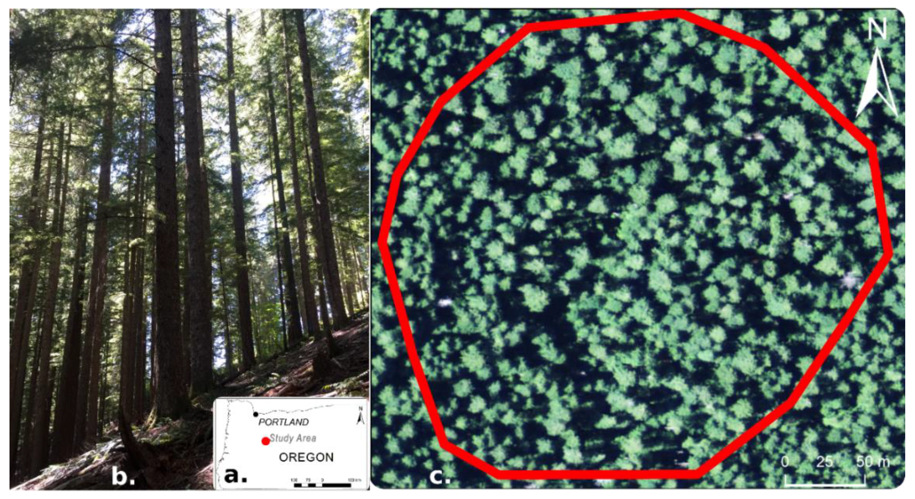
The proposed procedure for geo-referencing trees was applied to a 7.1 ha plot located inside a 12.3 ha Douglas-fir (Pseudotsuga menziesii Mirb.) stand from the HJ Andrews Experimental Forest in western Oregon (Figure 2a). The soils on the site are from the Browder, hummocky-Cadenza complex, with more than 30 cm of silt loam. The B horizon, almost stone-free, is made of silty clay loam. The C horizon appears below 1.0 m depth. The soils are at least moderately well-drained, which lead to superior productivity and allows active forest management. According to Means and Helm [17], the site index for Douglas-fir at base age 50 is 34 m. The average dominant and codominant height is 35 m. Besides Douglas-fir, some western red cedar (Thuja plicata Donn) are present in the stand. The stand has a southern aspect, with slopes between 0° and 35°. There is limited understory, which allows for unobstructed view of all the trees at least 10 m away from any point within stand (Figure 2b). The clear sight within the stand allows the capture of the lower portion of the stems using red-green-blue (RGB) cameras.

2.2. Procedure

2.2.1. Tree Segmentation from the Above Canopy Acquired Point Clouds

To locate the trees, we use georeferenced point clouds. The point clouds can be developed from active or passive sensors. Passive sensors, particularly CCD (i.e., charge-coupled device) or CMOS (i.e., complementary metal-oxide semiconductor) that record RGB images, are attractive to forestry applications because of robustness and low-cost (e.g., at the time when the paper is written a Phantom 3 Standard by DJI, which includes the vehicle and the sensor, is approximately 500 USD). Therefore, we produced a point cloud from the RGB images acquired with the unmanned aerial system DJI Phantom 3 Professional, which is a quadcopter equipped with a 1/2.3″ CMOS sensor capable of recording 12.4 mega pixels pictures. The Phantom 3 Professional is equipped with a satellite positioning system that is GPS and GLONASS capable, with a manufacturer stated accuracy of 1.5 m horizontally and 0.5 m vertically. To ensure precise positioning of the PPC, three ground control points identified with 1 m × 1 m crosses were placed in the middle of the road bordering the stand. The position of the center of each cross was estimated with a Trimble Geo XH, which has a stated accuracy of 0.3 m. We execute the flight at an average above ground elevation of 100 m and using 80% forward-overlap and 60% side-overlap, to ensure proper 3D reconstruction of the stand. We created the point cloud using structure-from-motion [18,19,20,21], as implemented in Agisoft version 1.3.4 [22]. The Agisoft parameters used to process the images were based on the recommendations of Fang and Strimbu [15,23].
We infer stem location from tree crowns, which were identified using the point cloud created from the above canopy images. Because the point clouds are georeferenced, the tree crowns will also be georeferenced. Once the tree crowns were delineated, we consider that the stem is located at the tallest point within the crown. However, the coordinates of the tallest point within the crown does not necessarily accurately represent the actual coordinates of the lower portion of the stem, as trees often respond opportunistically to canopy openings to access light. Therefore, an adjustment is needed, as the highest point would likely not be located on top of the axis of the lower portion of the stem, the portion that is visible from the ground. To ensure that only the points describing a tree are used for the correction of stem location we assumed that the stem is located close to the centroid of the crown projected area. To represent the assumption, we considered that the stem cannot be further from the Cartesian coordinates of the tallest point within the crown by more than 1/3 the radius of a circle with an area equal to the crown projected area (similar to the centroid of a triangle):
d i s t a n c e s t e m = A r e a c r o w n / π / 3
Therefore, the stem position will be the highest point within a circle centered in the crown centroid and with the radius computed with Equation (1). The location of the stem, depends not only on the crown shape, which is responsible for the centroid position, but also on the point density, the higher the density, the closer the stem location would be to the location of the highest point inside the canopy. To avoid inclusion of parameters that are not necessarily directly related to the main study objective, we have created PPC with a density of at least 30 points/m2. Such a high density, particularly for the PPC, which are focused on the outer part of the canopy, will ensure that the tallest return is close to the terminal bud. For actively managed forest the terminal bud is not horizontally offset more than 2 m from the stump [24], which will warrant the presence of the highest point and the stem within the same point cloud defined by the projected crown. To ensure the correspondence between the above and below canopy stems, only the low elevation points within the distance defined by Equation (1) are considered. We considered the points from the first quartile of heights as low-elevation points, which contain more stem points than the other quartiles. Furthermore, to reduce the chance of classifying terrain and small shrubs as trunk, only the points above 2 m from the ground are included in computations. The final (x, y) coordinates of the stem are the mean (x, y) coordinates of the points from the first quartile (i.e., low-elevation), weighted with the horizontal distance to the tallest point (an approximation of the top of the tree).
Several algorithms are available for individual tree crown segmentation (i.e., projected crown on the datum), none operating without error [4,5,25]. For this study, we used the oriented weighted graph algorithm of Strimbu and Strimbu [5], which currently seems to perform with minor errors given limited resources, and Dalponte and Coomes [6], which was proven to produce relatively accurate results. Because geo-referencing is executed by matching the trees segmented from above canopy with the trees from below canopy all the trees from the stands should be identified. Therefore, commission errors (i.e., false positive) are preferred over omission errors (i.e., false negative). Nevertheless, to ensure real-time computations, the commission errors should be kept minimal, otherwise, any local maxima could be considered a tree. The individual tree crown segmentation algorithms of Strimbu and Strimbu [5] and Dalponte and Coomes [6] perform with high accuracy if the point cloud is normalized, meaning the ground elevation is subtracted from each point. Several algorithms are available for ground normalization, almost all requiring point classification. However, the PPC created with Agisoft is not classified, therefore we have used an alternative algorithm, implemented in Quick Terrain Modeler [26], which is an iterative selection of minimum elevation points within a predefined grid.
We preferred the classification from Quick Terrain Modeler over other algorithms, as it is executed very fast (i.e., less than 1 s on a Dell Precision 7810 with an Intel Xeon E5-2630 v3 CPU and 32 Gb RAM) and supplies results comparable with more sophisticated implementations, such as TerraScan [27]. To ensure that not only speed but also point quality is present in the classification we compared the points classified with Quick Terrain Modeler with the classification performed by lastools [28] and PDAL [29]. The three classifications were similar in term of number of points and produced terrain models comparable with the US Geological Service models [30], which supported our choice for points classification. The tree segmentation algorithm based on oriented weighted graphs of Strimbu and Strimbu [5] as implemented in TrEx ver. 022 [31] and of Dalponte and Coomes [6], as implemented in LidR package of R ver. 3.5.1 [32]. The two segmentation algorithms produced similar results, but we have chosen the results supplied by Strimbu and Strimbu [5], as it outperformed the Dalponte and Coomes [6] algorithm when measured by omission, commission and overall accuracy error (i.e., omission error was 6% vs. 8%, commission error was 10% vs. 12%, and overall accuracy was 16% vs. 20%).

2.2.2. Generation of Point Clouds from below Canopy Images

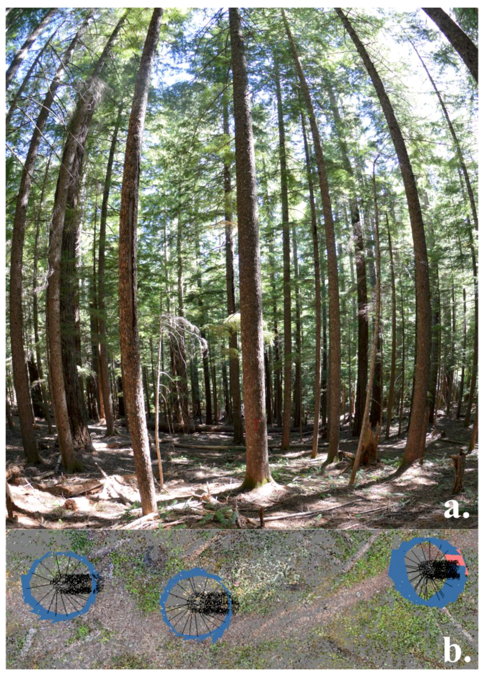
Similarly to the above canopy point cloud, the trees seen from the ground will be 3D reconstructed from images. The only difference between the generation of point clouds consists in the view point: nadir for above canopy and perspective for below canopy. To capture a large section of the bole of the trees a wide-angle lens is preferred. In this study we have used two cameras: one with no GPS (i.e., Nikon D3200) and one with GPS (i.e., GoPro Hero 5). The Nikon camera was equipped with the Sigma EX 10 mm fisheye lens, to capture the entire tree in one image. The images were captured with a resolution of 24.06 mega pixels with no flash (Figure 3a), which resulted in high ISO sensitivity for some images (e.g., 400). To reconstruct the trees, we have captured at least 20 images at locations approximately 10 m apart, almost uniformly distributed inside the stand. A total of 20 locations were captured, as trees at the edge of the plot were constructed from the images captured from locations within the plot (approximately a 6 m buffer inside the plot). The images recorded at each location were approximately evenly distributed along a circle (i.e., ~20° between two adjacent images) with camera pointed away from location (Figure 3b). A similar procedure, and consequently point cloud, was obtained from the images captured with GoPro camera. We produced separate point clouds for each device by processing the images with Agisoft version 1.3.4 [22] using the parameters of Fang and Strimbu [15,23]. The major difference between the two-point clouds (i.e., from Nikon and from GoPro) being their positioning, one in relative coordinates (i.e., disconnected from reality-Nikon), and the other relatively positioned in the correct region (i.e., no accuracy—GoPro).

2.2.3. Identify the Relative Coordinates of the Trees from below Canopy Point Cloud

The PPC generated at each location under the canopy rendered at least 10 trees, but they were not accurately geo-referenced. To position them, even in relative coordinates, the trees must be identified. To extract the trees from the PPC we have implemented a two-step procedure: first, eliminate the points that most likely are not the stem, and second, locate the most likely position of the stem within the thinned point cloud. For terrestrial lidar scans, there are many procedures that identify the points that are not stem. The procedures used on lidar data have limited success on PPC because the point cloud contains more noise. However, lidar does not contains colors, which are available with the PPC. Therefore, we considered that points that are green (i.e., leaves) or blue (i.e., sky), are not stem, therefore, should be eliminated from stem identification. Images captured throughout the stand facing different directions record tones varying from location to location. Therefore, the color of the PPC created at each location should be normalized, to ensure consistency throughout the stand. Among the multiple algorithms [33,34] and equations available for normalization we have used the feature scaling [35], which does not produce unnatural appearances, an issue of complex algorithms, while homogenizing the hue throughout the stand:
n o r m a l i z e d h u e = h u e   v a l u e in ( h u e   v a l u e ) max ( h u e   v a l u e ) min ( h u e   v a l u e ) × 255
After normalization of each wavelength, we differentiated the stem from non-stem points by implementing two constraints (Equations (3) and (4)), one operating in absolute values and one in relative terms. The restriction using absolute values (Equation (3)) identifies a non-stem point as one for which the normalized color is mostly blue or green (hue of blue and green > 127) while red have a reduced presence (hue of red ≤ 127). The constraint using relative terms (Equation (4)) identifies non-stem points as the ones for which both blue and green have larger hues than red.
if   { n o r m a l i z e d b l u e > 127   or   n o r m a l i z e d g r e e n > 127 n o r m a l i z e d r e d 127   then   non - stem
if normalizedblue > normalizedred or normalizedgreen > normalizedred then non-stem
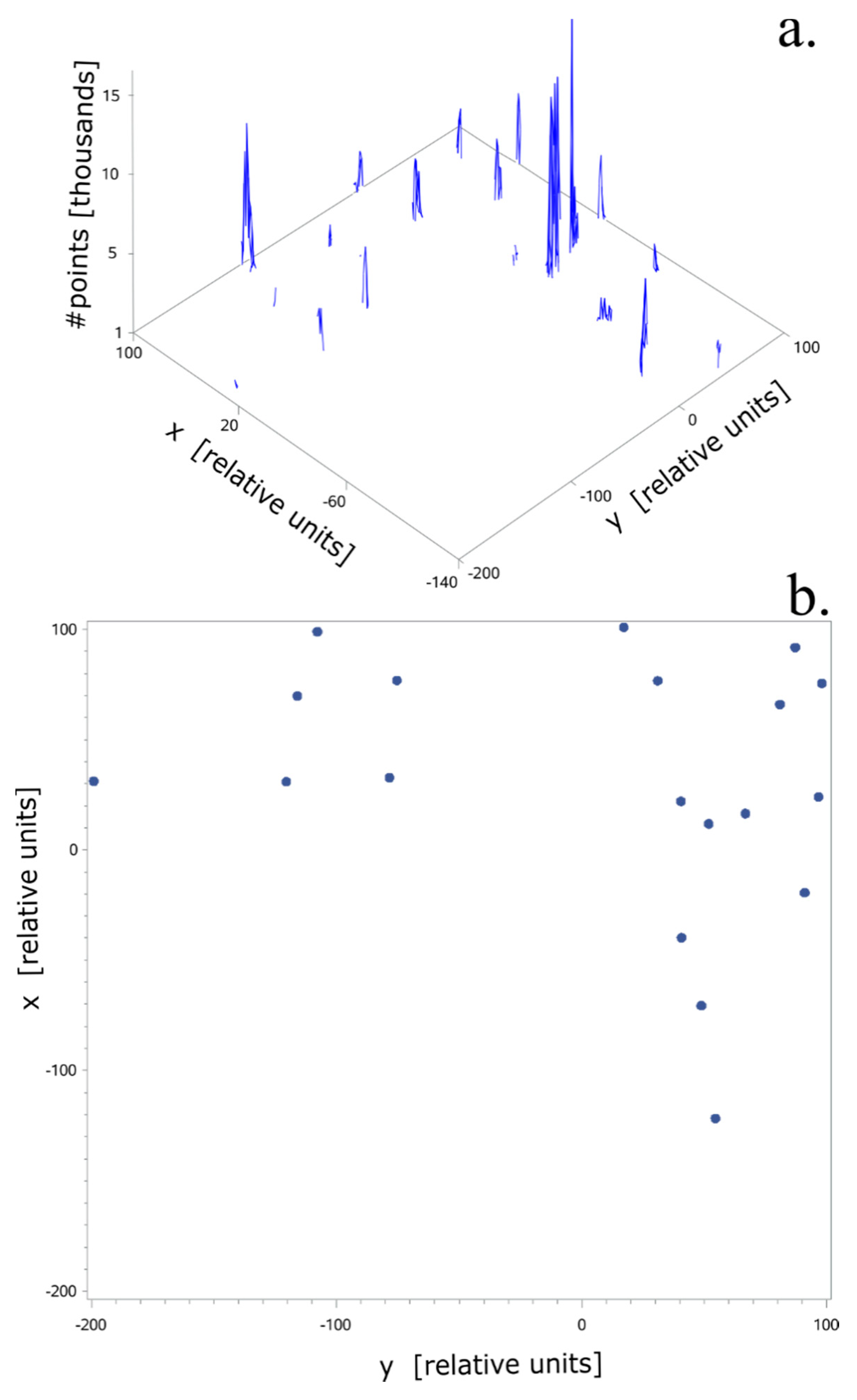
To identify the location of the stems within the filtered PPC we developed a simple and fast procedure that is accurate enough, considering that the final identification of the trees will be executed by combining the above canopy information with the below canopy information. Our procedure relies on the assumption that trunks will be represented by more points than other forest features; therefore, a counting of points across an area should display the trunks as spikes. We represented a tree by the center of the stem; therefore, for each spike we computed its centroid. To identify each stem, we have used hierarchical clustering [36], with the measure of similarity being the average linkage (distance). We preferred the average distance over other measures of similarity because it is relatively robust to outliers and directly computes the location of each tree. The number of clusters, namely the number of trees, was chosen using the property that the proximity measure changes exponentially with the number of clusters [37]. We considered that a sudden change in proximity measure followed by a relatively flat line indicates that the significant number of clusters was achieved (similar to the screen test). We executed cluster analysis in SAS 9.4 [38], as it has a more intuitional interface than other packages.

2.2.4. Match the Inaccurate or Unreferenced Trees with the Georeferenced Trees

The final step in geo-referencing the trees segmented from under the canopy images consists in their matching with the trees segmented from above canopy. Among the various approaches that matches trees, we have chosen a point set registration algorithm [39,40,41,42], namely the nonrigid transformation of Ma et al. [43]. Several algorithms are commonly used for point set registration, the Iterative Closest Point of Besl and McKay [44], the coherence point drift algorithm of Myronenko and Song [45], the robust point-matching-preserving local neighborhood structures proposed by Zheng and Doermann [46], and the Kuhn–Munkres algorithm [47], which were proven to perform well in fingertip detection [48,49], phalanges [50], and in general on problems that can be represented by graphs [51,52]. The Kuhn–Munkres algorithm has a cubic complexity [47], which makes it attractive for solving combinatorial problems encountered in many forestry problems. However, the Kuhn–Munkres algorithm is sensitive to noise, which leads to a reduced accuracy in tree position. Because the trees located from above-canopy and below-canopy PPC are not accurately positioned, the Kuhn–Munkres algorithm is not the best suited for the geo-referencing problem at hand. Therefore, we use the non-rigid point-matching algorithm of Ma et al. [43], which can accommodate outliers and inaccuracy in data, more specifically small discrepancies between the coordinates of the trees segmented from above canopy and the trees segmented from below canopy. The lack of accuracy in tree position is present in both PPCs: from above canopy, as the tallest point within the tree crown is likely not located on the stem axis, and from below canopy, as the location of the tree is probably not the average of the x and y coordinates of the points filtered to represent the trunk. Furthermore, the non-rigid algorithm is designed to match sets with different number of elements [53], in our case trees, which is exactly the situation encountered in real situations.
The algorithm of Ma et al. [43] estimates the transformation f, of the tree located under the canopy to their corresponding trees seen from above canopy using a cost function, called L2E, which minimizes the L2 distance between the densities defined by the transformation f. The algorithm operates in two steps, first feature descriptors, such as shape context, of the tree location are established, and second, the transformation of the unreferenced trees to the georeferenced ones is computed using the robust estimator L2E, a L2 measure minimizing estimate. The L2E was tested on linear regression and estimated the correct values for the slope even when half of data were outliers, whereas the maximum likelihood estimators supplied a reliable solution only for a limited number of outliers [43]. In our study, we have used the Matlab [54] implementation of the algorithm by Ma et al. [43], as it relies on fast and near-optimal implemented computational algorithms. The logical structure of the algorithm is the following [43]:
Step 1
Input the location of the trees, as seen from below, { x i } i = 1 n , and as seen from above, { y j } j = 1 l
Step 2
Compute feature descriptors for the location of the trees seen from above { y j } j = 1 l
Step 3
Start a recursive procedure with a preset number of iterations
Step3-1 
Compute feature descriptors for the relative location of the trees seen from below { x i } i = 1 n
Step3-2 
Estimate the initial correspondences based on the feature descriptors of two-point sets locating the trees, one from above and one from below
Step3-3 
Solve the transformation f, f ( x ) = i = 1 m Γ ( x i ,   x ˜ i ) c i , which warps the set of points representing the trees seen from below (the model point set) to the set of points representing the trees seen from above (the target point set). The Γ is a positive defined matrix Γ: Rd × RdRd×d and { x ˜ j } j = 1 m is a random subset of points to have nonzero coefficients in the expansion of the solution of f. The solution of f is found using the following steps:
Step3-3a 
Input the annealing rate γ, and the parameters that control the smoothness of the transformation f, β and λ. Ma et al. [43] argued that the method is robust to parameter changes, therefore we have chosen the values recommended by Ma et al., namely γ = 0.5, β = 0.8 and λ = 0.1.
Step3-3b 
Construct the Gram matrix Γ and matrix U, where
Γ i j = Γ ( x ˜ i , x ˜ j ) = e β x ˜ i , x ˜ j
U i j = Γ ( x i , x ˜ j ) = e β x i , x ˜ j
Step3-3c 
Initialize C and σ2 where
σ2 is the variance of the point correspondence, computed as yif(xi)
d is the dimension of the coefficient ci from the C, the coefficient matrix m × d used in conjunction with the Gram matrix: C = (c1, …, cm)
Step3-3d 
Start deterministic annealing [55] aimed at minimization of the function
L 2 C ( C , σ 2 ) = 1 2 d ( π σ ) d / 2 2 n i = 1 n 1 2 d ( π σ ) d 2 e y i T U i C 2 σ 2 + λ tr ( C T Γ C )
where CT is the transpose of C, and tr is the trace of the matrix CTΓC
using the quasi-Newton algorithm with C as the old value and the gradient L 2 E ( C , σ 2 ) C ,
Step3-3d-I: 
update C ← arg minC L2E(C, σ2)
Step3-3d-II: 
anneal σ2 = γ σ2
Step3-3e 
Select the solution of f ( x ) = i = 1 m Γ ( x i , x ˜ i ) c i obtained by minimizing L2E
Step3-4 
update the location of the trees seen from below (model point set) { x i } i = 1 n { f ( x i ) } i = 1 n
Step 4
Stop when the preset number of iterations is reached
Step 5
The georeferenced trees seen from below have the location { f ( x i ) } i = 1 n

2.2.5. Robustness of Tree Georeferencing to Missing and Erroneous Positioned Trees

We preferred the algorithm of Ma et al. [43] because it has two properties that makes it suitable for forestry applications: it accurately models the transformation required to align the point sets without sacrificing computational complexity (i.e., linear complexity in the number of correspondences), and it is robust to noise, outliers, and missing points. The final location of the trees is established by preserving the relative distances among the trees determined from the below-canopy PPC but rotated, translated, and expanded or contracted according to the geo-referenced trees from above-canopy PPC. For our research, the main issue is the inaccurate location of trees from both above and below canopy rather than on missing trees. Therefore, besides the results supplied by the field data, we tested the robustness of the algorithm to erroneous coordinates using a simulation that considered all trees as wrongly positioned.
The erroneous data is not the only issue impacting the performances of the Ma et al. [43] algorithm. Besides the intrinsic parameters required by the algorithm, such as annealing rate, γ, the width of the range of interaction between samples (i.e., neighborhood size), β, and the control of the strength of regularization, λ, the algorithm depends also on the number of outliers and the trees to be matched. For the case when trees were wrongly located we considered five mean errors ranging from 1 m to 5 m, in increments of 1 m. The error was allocated to individual trees positioned using the point cloud developed from the nadir images, as they are georeferenced. In absence of the contrary, we assumed that errors are uniformly distributed with mean {1, 2, 3, 4, 5} and variance 1. To assess the impact of the missing trees and the number of the matching trees, as mentioned by Ma et al. [43], we considered that only 70% or 80% of the trees identified from above are found in the unreferenced trees (i.e., below). Therefore, we created a 5 × 2 factorial experiment to assess the robustness of the geo-referencing procedure to positional errors and missing trees.

3. Results

3.1. Geo-Referencing Trees Using Real Data

Initial Geo-Referencing

We produced the PPC from the images collected above-canopy based on the study of Fang and Strimbu [15]. The options used for image alignment and point densifications were: half size images, 100,000 key points, 40,000 tie points, and the outliers identified assuming that no meaningfully small details are present (i.e., the aggressive depth filtering option). The final PPC has approximately 2,600,000 points, with an average point density of 37 points per square meter. The PPC geo-reference accuracy depends on the location of the ground control points [56], which in our study where not uniformly spread throughout the stand; therefore, errors are expected. Nevertheless, the magnitude of the geo-referencing error is likely to be significantly less than the tree-matching error, as non-rigid matching algorithms, including the one of Ma et al. [43], are not perfect.
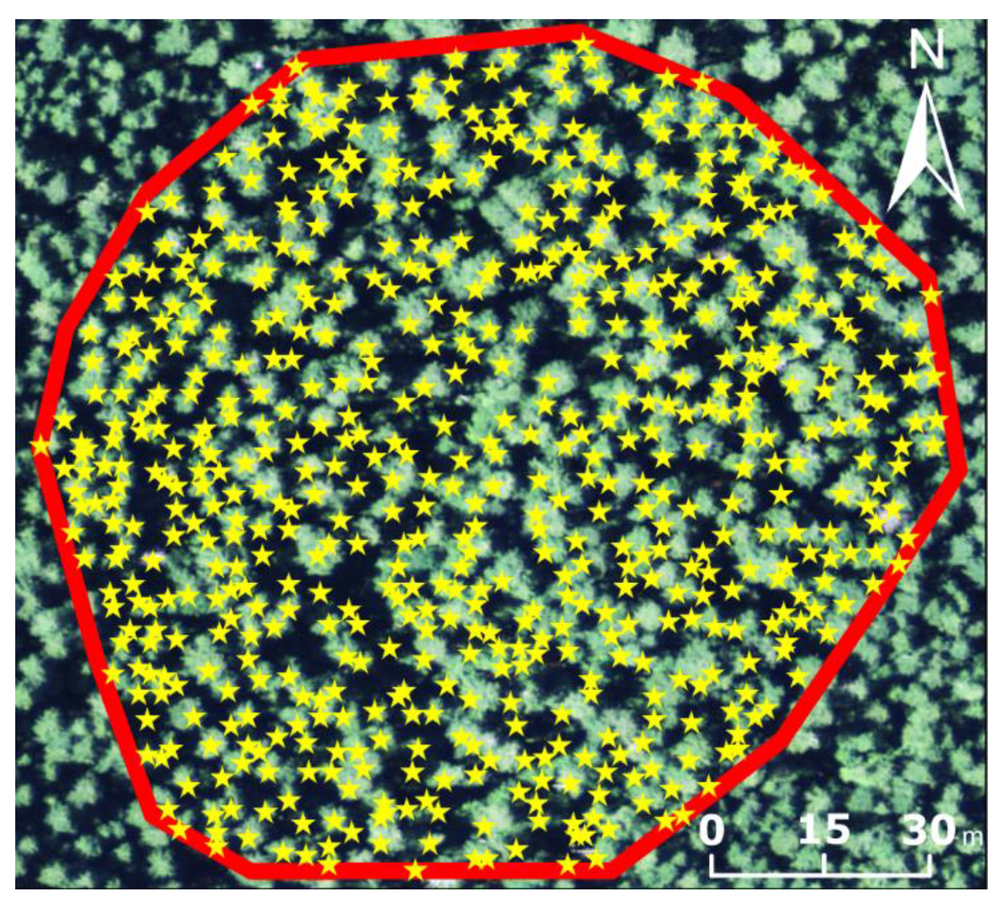
To extract trees from the above-canopy PPC with TrEx we followed the recommendations of Strimbu and Strimbu [5]. The set of parameters used to extract trees without a significant number of false positives were: a 1 m cell for computing maximum elevation, a Gaussian smooth of 0.7 pixels, 32 height levels, and 4 adjacent cells. The graph created by TrEx had weights of 50% for level degree and 50% for top distance, whereas the trees were finally delineated using a 70% best sufficient parent and more than 10 pixels for each crown (Figure 4).
The total number of trees extracted by TrEx from the normalized PPC was 641 trees; out of which few are not necessarily actual trees, but branches mistakenly identified as trees. The initial location of each tree was selected to be the coordinates of the highest point within the crown. Once the trees were extracted, TrEx delineated their crown by tracing the pixels identified within the oriented weighted graph as belonging to neighboring trees. The final coordinates of the trees segmented from the above canopy PPC were determined using the lower quartile of the points above 2 m that were located inside the circle centered in the initial tree location and with radius computed with Equation (1). The final coordinates differ, on average, 0.45 m from the initial tree coordinates (i.e., coordinates of the highest point within the crown), as computed by TrEx. The differences range from 0.1 m to 1.7 m.
The parameters used to reconstruct the PPC from below-canopy images were based on Fang and Strimbu [23], but adjusted to produce fast results, less than 1 min per location. Therefore, to align the images we have used only ⅟16 × ⅟16 of each image (i.e., accuracy set to low), 40,000 key points, and 5000 tie points (Figure 5). Once the images were aligned, we densified the tie points by filtering the outliers assuming a lack of small meaningful details and ¼ of the linear information stored in each image. We integrate the PPCs generated at each location by first aligning them with the scale-invariant feature transform [57], and second by merging them.
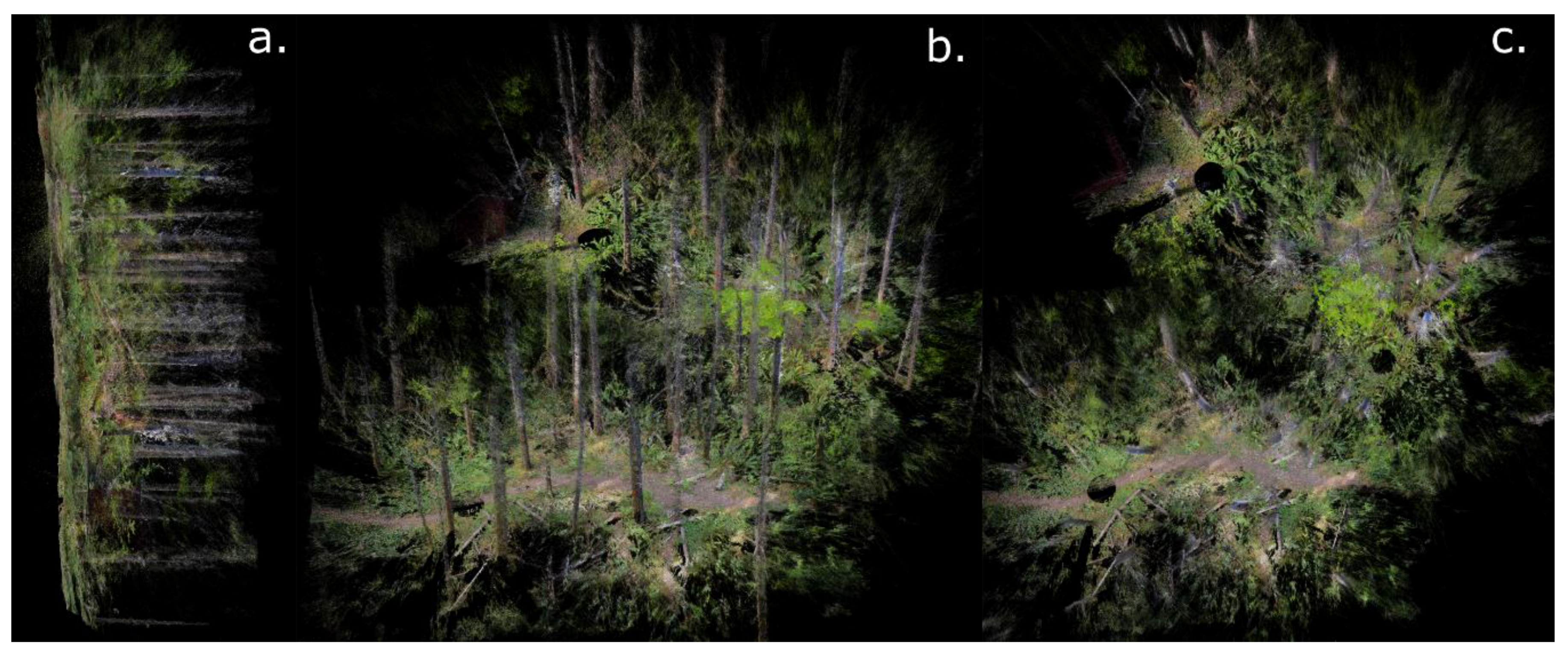
In the absence of reference points, the PPC produced with structure-from-motion [20,58,59,60] software will likely not have a nadir view. In addition, the PPC based on unreferenced images will have the relative coordinate system determined by the software assumptions and may place the point cloud in an unrealistic position, as we see in one location (Figure 5a), where the trees are positioned almost horizontally. Considering that nadir view of the PPC is required for stem identification, the initial PPC has to be rotated such that a coordinate system that ensure a top view is obtained. To position the PPC obtained from Nikon 5200 images (Figure 5a) in nadir view we manually rotated the point cloud by visual inspection (Figure 5c). A rotation with error is allowed, as a relative nadir view is sufficient for computing the stem location from the below-canopy PPC. The final geo-referencing (i.e., accurate nadir) is executed in the last step of the procedure. Manual rotation is executed only for the first location where images will be collected, as the rest of the PPCs will be successively aligned, and consequently having a nadir view of the trees. In comparison with the Nikon camera, the PPC produced from the Go Pro camera does not need any rotation, the point cloud being correctly oriented. Even though the position of the PPC from the GoPro is not accurate, the benefit of having an inaccurate GPS helps to eliminate a step needed for geo-referencing.
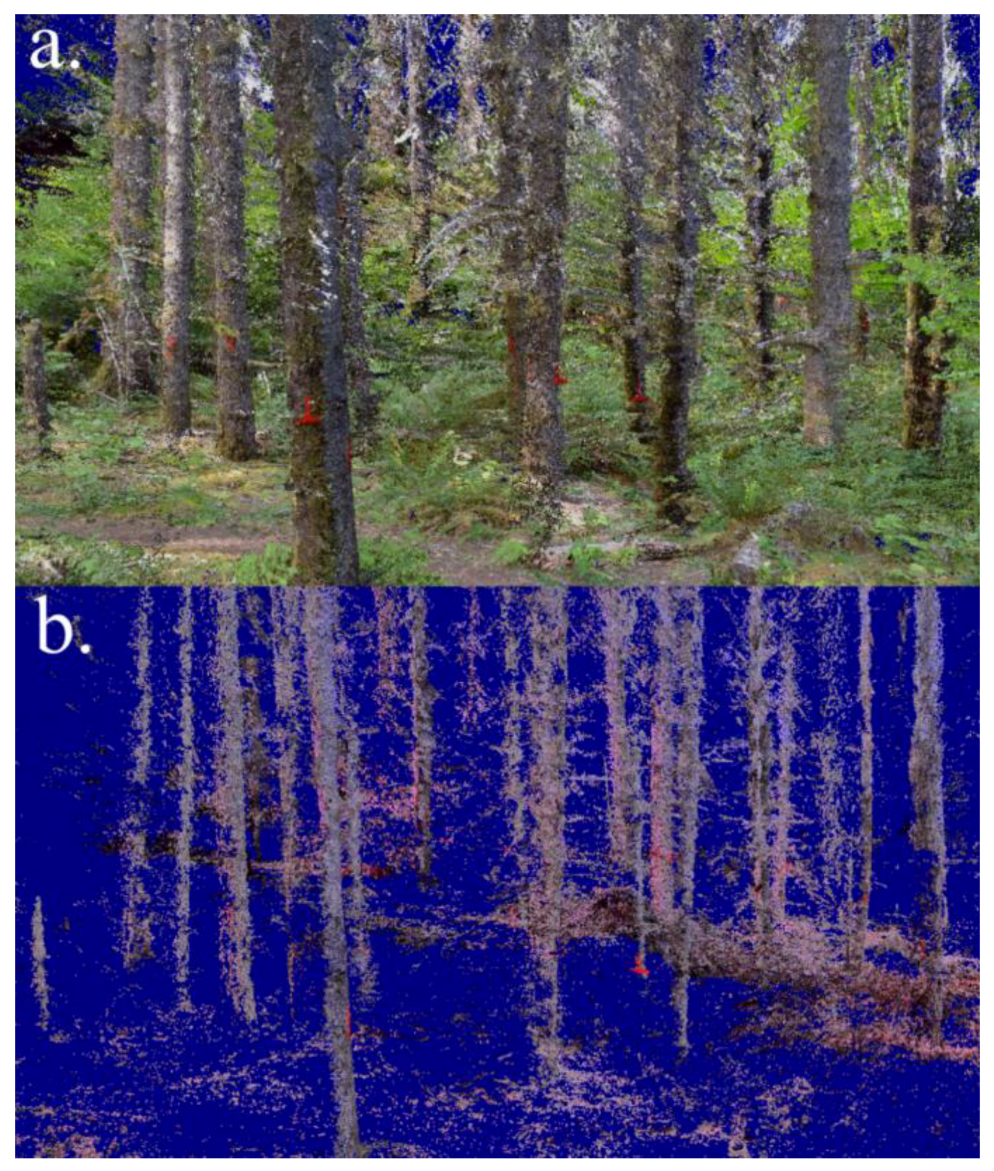
Our assumption that colors will separate the trunks from the non-trunks was shown to be true (Figure 6a is a selection from Figure 5c). The delineation was not clear on the 3D image (Figure 6b) but was obvious on the grid created from the count of points (Figure 7). Considering that the PPC is unreferenced, there is the possibility that the grid will produce statistics that are too coarse or too fine. To reduce the risk of meaningless statistics, we have selected a grid with unit cell size, in relative units, as Agisoft Photoscan [22] distributes the points relative to the location of the cameras. Cluster analysis found 612 trees from under the canopy PPC, and for the locations from Figure 6 only 19 trees.
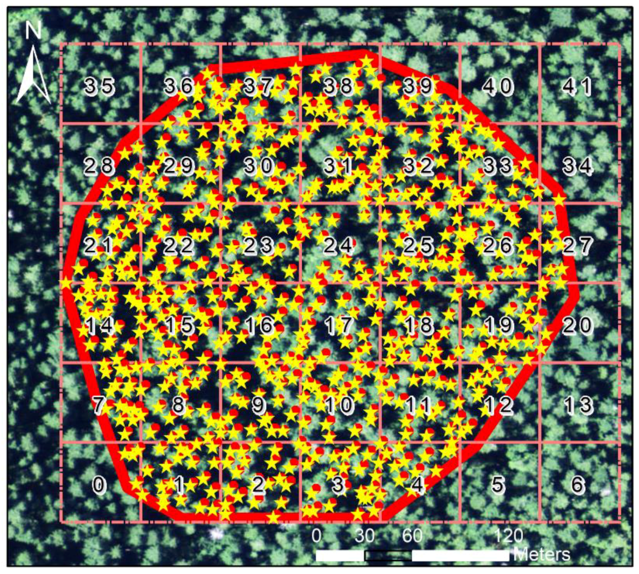
The point-matching of the 612 trees identified from below canopy with the 641 trees delineated from above canopy not only took a significant amount of time (i.e., more than 12 h) but also did not produce valid results, as the distance between some trees were more than 5 m. Therefore, we tried a different approach based on the observation of Ma et al. [43] that the number of trees under the canopy should not be large (in their simulations they used 15 points). Consequently, we divided the trees segmented from the PPC under the canopy in quadrants, each containing at most 20 trees. A simple-trial and error approach led to a grid with 30 m cell sizes. Matching the points from each quadrant into the 641 trees led to results even worse than before, as trees there spread throughout the 7.1 ha whereas, in reality, they are neighbors. To address this issue, we decided to reduce the size of the matching point sets by allocating the trees segmented from above the PPC into grid cells that would include at most 40 trees, twice as many as the number of trees from each cell with trees identified from below. This task is not difficult to implement when matching trees segmented from PPC developed from GoPro Hero 5 camera (i.e., low GPS precision), as each cell should be enlarged such that it would contain the cell from below and enlarged with the size of the manufacturer accuracy. Information about the accuracy of the GPS from the GoPro Hero 5 is not available from the manufacturer; therefore, we assumed that the accuracy is similar to other hobby GPS devices, such as Garmin or Magellan), which under the canopy is approximately 10 m. To ensure that all cells created from below PPC are georeferenced, we used a moving window with size 20 m (i.e., 10 m on each side) larger then under the canopy PPC grid, which led to a grid with 50 m cell sizes (Figure 8). However, this repeated process would take a significant amount of time, and at the end, the trees from all cells must be combined anyway. Therefore, we decided to select only five grid cells covering the trees identified from under the canopy PPC that are completely located inside the stand, four located close to the corners and one close to the centroid of the stand, namely 8, 11, 17, 22, and 32 (Figure 8). Furthermore, to reduce the computation time, we have selected from the trees segmented from the under the canopy PPC only the ones that are located inside the 30 m square within the five cells. The reduced number of cells used to geo-reference all the trees segmented from the below canopy PPC is of little significance, as the conversion from relative or imprecise coordinates to accurate coordinates is an affine transformation, namely a linear function. In theory, only one grid cell would have sufficed to georeference all the trees, but to ensure representability at the stand level and to correct for possible local distortions we have selected more cells evenly distributed through the stand. The original, imprecise, coordinates of the trees from the five cells, X, would be used to establish the translation vector, B, that converts to accurate coordinates, X ^ : X ^ = B × X . The translation vector, B is obtained by simple algebraic manipulations of the coordinates of the matched trees: accurate, X ^ and inaccurate, X (Equation (5)):
B = ( X ^ × X T ) ( X × X T ) 1
where ( X × X T ) 1 is the inverse of matrix X × XT.
The unmatched trees, Y, would have the coordinates corrected, Y ^ using B (Equation (6)):
Y ^ = B × Y
The usage of georeferenced images ensure that the grid cells used in the matching process contains some common trees. However, for the un-referenced PPC the location is relative; therefore, there is no overlapping of the grid created from trees segmented from above PPC with the grid created from the trees segmented from below PPC. To use the same procedure for unreferenced images that was employed for georeferenced images, we had to relatively overlap the two PPC, from above and below. To implement this task, first we matched the relative distance among the trees segment from above canopy PPC with the distance among the trees from segmented from below canopy PPC, and second, by rotating and translating the two set of tree locations (i.e., above and below) such that a relative overlap occurs. The first step ensures that the tree locations have similar magnitudes, as in the inaccurate georeferenced images, whereas the second step warrants that the grid cells created from above would include some of the trees segmented from below. Once the two sets of tree locations (i.e., above and below) are relatively aligned, we used the same process as for the relatively referenced trees to accurately locate the stems.
Irrespective the source of images to build the PPC (i.e., georeferenced images or not), we assessed the accuracy of procedure to georeference the trees by computing a matching error, defined as the mean distances between the actual and matched trees:
a c c u r a c y = ( i = 1 g j = 1 n g d i , j : a b o v e , m a t c h e d ) g × n g
where g is the number of the grids used to match the trees, in this study is 5
ng is the number of trees to be matched in grid cell g
di,j:above,matched is the distance between the location of the matched tree i obtained from the below-canopy PPC and the closest trees segmented from the above-canopy PPC, j.
The 2500 m2 grid cells, created from the trees segmented from the above canopy PPC, contain at least one tree (i.e., cells 34 and 40) and more than 20 trees, when they are completely inside the stand (Figure 8). Our results suggest that the accuracy of tree matching depends on the number of trees segmented from the above canopy PPC found inside the 2500 m2 grid cell and on the number of trees segmented from below canopy PPC found inside the 900 m2 grid cell, with values between 0.98 m and 1.15 m (Table 1). We noticed a constant trend that the accuracy is inversely related to the number of trees segmented from the under the canopy PPC, irrespective of the number of trees identified from above canopy PPC. The accuracy of tree matching was virtually the same (i.e., 1.07 m) for the five plots, but larger for all the trees [i.e., 1.09 m for the trees segmented from georeferenced images (GoPro) and 1.11 m for the trees segmented from unreferenced images (Nikon)].

3.2. Accuracy of the Georeferencing Procedure Using Simulations

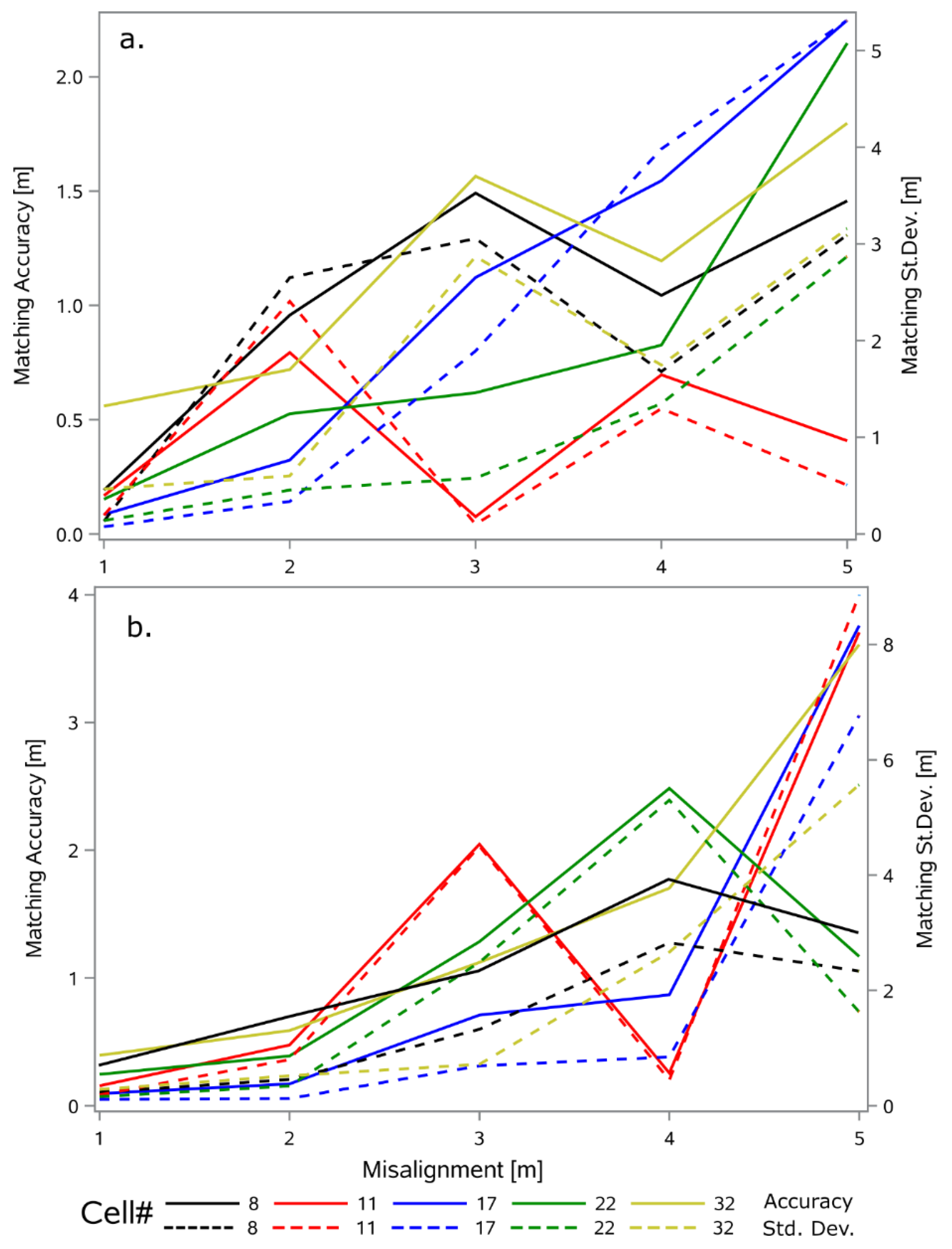
The factorial experiment designed to assess the impact of erroneous positioning of the trees, as well as of the missing trees, could not be implemented when the trees were georeferenced at once as a non-operational accuracy (>5 m) was present. Therefore, we have applied the same factorial experiment to the five grid-cells used for geo-referencing, as the selection of the initial positioning cells would define tree location accuracy. The results reveal that, irrespective the simulated overlap between the above and below canopy segmented trees (i.e., 0.7 and 0.8), for misalignment errors less than 2 m the trees will be geo-referenced with at most 1 m accuracy (Figure 9). Considering that usually mature trees are more than 1 m apart, a lack of alignment between the lower portion of the stem and the highest point likely to be achieved (i.e., <2 m) would lead to relatively accurate tree geo-referencing. However, the standard deviation of the tree geo-referencing depends on the overlap, as the more overlap, the more precise the tree location (Figure 9). In fact, for 70% overlap, the geo-referencing is operational only for misalignment errors less than 1 m (Figure 9a), whereas for 80% overlap, the misalignment error can be up to 2 m and the tree location is still with acceptable limits (Figure 9b).
The computation times for the five grid cells on a Dell Precision 7910 equipped with an Intel Xeon CPU E5-2630 [email protected] GHz is less than 10 s. The entire stand was geo-referenced in less than 1 min.

4. Discussion

To render trees using cameras under the canopy requires unobstructed visibility throughout the stand, particularly the lower portion of the stem. Good visibility of the stem ensures a fast and correct reconstruction of the trunk with structure-from-motion algorithms. The lack of understory vegetation is critical because it will not add noise around the stems, which helps extract the bole from the PPCs, irrespective the placement of the images, above or below canopy. The PPC created from images mirror reality and have all points colored. The presence of colors dramatically enhances processing of the PPC, permitting simple algorithms to supply faster and similar results to complex algorithms developed for colorless point clouds. If our color-based approach will still lead to a PPC with multiple non-stem points we will consider more sophisticated algorithms, but for mature Douglas-firs it seems that would not be needed. Visibility inside the stand is needed not only for 3D reconstruction of the stems but also for correct positioning of the trees segmented from above canopy PPC. Our results show that errors of more than 1 m in locating trees from above can lead to inaccurate results.
The non-rigid point-matching algorithm of Ma et al. [43] accommodates the lack of accuracy in positioning the trees from the above-canopy PPC and the below-canopy PPC, which makes it more attractive than the Kuhn–Munkres algorithm. However, its flexibility also possesses challenges, as the trees are not matched properly if multiple combinations are available. To address this issue, we reduced the size of the problem by overlaying a grid on the tree segmented from above PPC aiming at matching only a reduced set of trees. While the decrease in the number of combinations proved beneficial, as it solved the matching accuracy, it introduces an extra level of complexity. The addition of the grid does not ensure a complete solution, as it is possible that, in some situations, not all the trees identified from the below-canopy PPC would fall inside one grid cell. However, we demonstrated that our approach is operational and, perhaps more importantly, it is simple and easy to implement, given the current technology.
Our results show that irrespective the existence of a positioning device (such as GPS) trees would be accurately georeferenced. However, the lack of geotagged images requires extra steps, which increase the computation time and are prone to errors that could impact the accuracy of tree positioning. Our findings show that that absolute accuracy of trees location segmented from the below canopy PPC is not relevant, what is important is the relative position of the stems. It is the relative position that allows the usage of an area adjusted simultaneously to the trees delineated from the above-canopy PPC and below-canopy PPC, which ensures the matching accuracy. Additionally, the PPC that is spatially located eliminates its rotation, as the point cloud has a nadir view.
The proposed geo-referencing procedure of trees under the canopy with no or in-accurate GPS devices produces the expected results relatively fast. All the computations directly related to geo-referencing are executed in less than 1 min. The final location of the trees is sensitive to the misalignment between the tree top and lower bole, which for accurate positioning cannot be larger than 2 m. The requirement for aligning the top with the bottom of tree is necessary not only for overall accuracy but also because beyond 2 m, the standard deviation increases to levels that are not operational anymore. However, advances in sensor development would most likely reduce the difference between the stem and tree top coordinates. Furthermore, the inclusion of more trees segmented from the under the canopy PPC increases the accuracy of geo-referencing. Consequently, any improvement in locating the trees would reflect in a more accurate and less variable tree positioning.
We expect the georeferencing procedure that we developed to supply accurate results for deciduous species, especially if the images are acquired during the leaf-off season. The lack of leaves allows reconstruction of the trees with PPC containing sufficient stem points to ensure that the misalignment between the top of the tree and the lower part of the bole is less than 2 m. In fact, we expect that the difference between the two locations (i.e., tallest point and lower bole centroid) to be less than 1 m, as the globular shape of the crown would likely produce a maximum elevation point closer to the stem axis even when crown moves. It is possible that for the leaf-off season, the selection of the points from the lower quartile as basis to estimate the location of the trees from below canopy images could be replaced with the lower quintile, as more stem points are available.

5. Conclusions

Positioning trees on a geo-referenced map based on under-the-canopy measurements is challenging and time-consuming. The advancement in computer vision allows 3D reconstruction of the entire stands, but significant difficulties are encountered when they are placed on geo-referenced maps. Therefore, in this study we focused on geo-referencing trees segmented from under the canopy images that contains either no spatial coordinates or low accuracy GPS values. Furthermore, we aimed at developing a procedure for geo-referencing 3D point clouds representing the lower section of the trunk that is relatively inexpensive, fast, and accurate using only RBG images. Our procedure is based on using the coordinates of the trees seen from above canopy to position the same trees seen from below canopy. Multiple photogrammetric point clouds are developed using structure-from-motion implemented in Agisoft [22], one acquired with an unmanned aerial vehicle (i.e., DJI Phantom 3 Professional) that will be used for tree segmentation from above canopy, and multiple at different locations throughout the stand, which will serve to identify the absolute location of the trees as seen from below canopy. The location of the trees segmented from below canopy are matched with the location of the trees extracted from above canopy, in the sense that their coordinates will be affine-transformed based on the georeferenced trees. We segmented the crown of the trees from above using TrEx 022 [5] and estimated the coordinates of the trunks by using the lower quartile of the points 2 m above ground but within the horizontally projected crown. The location of the stems developed from under-the-canopy images were estimated with hierarchical cluster analysis [36] executed on the color filters points (i.e., green and blue points eliminated). We matched the trees identified from above canopy with the trees from below canopy with the non-rigid point-matching algorithm of Ma et al. [43]. We found that tree matching algorithm of Ma et al. [43] is too flexible, in the sense two sets of trees will almost always will be matched, given a preset accuracy. To ensure correct results, we reduced the number of the trees to be considered for matching by dividing the trees segmented from above using a quadratic grid of 50 m. The trees segmented from the below canopy PPC falling inside a 50 m cell buffer with the manufacturer GPS accuracy were matched with the trees from the 50 m grid-cell. For a misalignment of the trees less than 2 m the trees are mapped with an average accuracy of less than 1 m. The proposed procedure is relatively fast, as for a 7.1 ha stand, the entire matching process is approximately 1 min (on a Dell Precision 7910 equipped with a CPU Intel® Xeon® E5-2630 v3 and 32 GB RAM). The pair-matching procedure depends on the number of trees to be matched; the larger the number of trees, the larger the accuracy. A limitation of the proposed procedure is the need to rotate the point clouds generated from unreferenced images, such that a close to nadir view is obtained. However, this weakness is eliminated when geotagged images are used during the structure-from-motion reconstruction. The accuracy of positioning the images captured under the canopy is irrelevant, because the main purpose is to ensure the nadir view of the point clouds. We think that tree matching is possible to be executed in real-time if SLAM algorithms [61,62,63] are used for 3D tree rendering instead of structure-from-motion algorithms [57,64,65]. Furthermore, accurate geo-referencing of tree stems could help improve species identification when analysis is executed data fusing spectral information with locational data [66,67,68].

Author Contributions

Conceptualization, B.M.S.; Methodology, B.M.S. and C.Q.; Software, B.M.S. and C.Q.; Validation, B.M.S., C.Q., and J.S.; Formal Analysis, B.M.S. and C.Q.; Writing-Original Draft Preparation, B.M.S. and J.S.

Funding

This research was funded by the National Institute of Food and Agriculture, U.S. Department of Agriculture, grant number 2019-67019-29462 and McIntire Stennis project OREZ-FERM-875.

Acknowledgments

We would like to thanks he H. J. Andrews Experimental Forest for providing accommodation and support in collecting the data.

Conflicts of Interest

The authors declare no conflict of interest. The founding sponsors had no role in the design of the study; in the collection, analyses, or interpretation of data; in the writing of the manuscript, and in the decision to publish the results.

References

  1. Kershaw, J.A.; Ducey, M.J.; Beers, T.W.; Husch, B. Forest Mensuration, 5th ed.; Wiley Blackwell: Hoboken, NJ, USA, 2017; p. 613. [Google Scholar]
  2. Weiskittel, A.R.; Hann, D.W.; Kershaw, J.A.; Vanclay, J.K. Forest Growth and Yield Modeling; Wiley-Blackwell: Chichester, UK, 2011; Volume 430, p. 415. [Google Scholar]
  3. Popescu, S.; Wynne, R.H.; Nelson, R.H. Using lidar for measuring individual trees in the forest: An algorithm for estimating the crown diameter. Can. J. For. Res. 2003, 29, 564–577. [Google Scholar]
  4. Kaartinen, H.; Hyyppä, J.; Yu, X.; Vastaranta, M.; Hyyppä, H.; Kukko, A.; Holopainen, M.; Heipke, C.; Hirschmugl, M.; Morsdorf, F.; et al. An international comparison of individual tree detection and extraction using airborne laser scanning. Remote Sens. 2012, 4, 950–974. [Google Scholar]
  5. Strimbu, V.F.; Strimbu, B.M. A graph-based segmentation algorithm for tree crown extraction using airborne lidar data. ISPRS J. Photogramm. Remote Sens. 2015, 104, 30–43. [Google Scholar] [CrossRef]
  6. Dalponte, M.; Coomes, D.A. Tree-centric mapping of forest carbon density from airborne laser scanning and hyperspectral data. Methods Ecol. Evol. 2016, 7, 1236–1245. [Google Scholar] [CrossRef] [PubMed]
  7. Li, W.; Guo, Q.; Jakubowski, M.K.; Kelly, M. A new method for segmenting individual trees from the lidar point cloud. Photogramm. Eng. Remote Sens. 2012, 78, 75–84. [Google Scholar] [CrossRef]
  8. Wells, L. A Vision System for Automatic Dendrometry and Forest Mapping. Ph.D. Thesis, Oregon State University, Crovallis, OR, USA, 2018. [Google Scholar]
  9. Azizi, Z.; Najafi, A.; Sadeghian, S. Forest road detection using lidar data. J. For. Res. 2014, 25, 975–980. [Google Scholar] [CrossRef]
  10. White, R.A.; Dietterick, B.C.; Mastin, T.; Strohman, R. Forest roads mapped using lidar in steep forested terrain. Remote Sens. 2010, 2, 1120–1141. [Google Scholar] [CrossRef]
  11. Fritz, A.; Kattenborn, T.; Koch, B. Uav-based photogrammetric point clouds—Tree stem mapping in open stands in comparison to terrestrial laser scanner point clouds. Int. Arch. Photogramm. Remote Sens. Spat. Inf. Sci. 2013, 40, 141–146. [Google Scholar] [CrossRef]
  12. Wainwright, H.M.; Liljedahl, A.K.; Dafflon, B.; Ulrich, C.; Peterson, J.E.; Gusmeroli, A.; Hubbard, S.S. Mapping snow depth within a tundra ecosystem using multiscale observations and bayesian methods. Cryosphere 2017, 11, 857–875. [Google Scholar] [CrossRef]
  13. Pierzchała, M.; Talbot, B.; Astrup, R. Measuring wheel ruts with close-range photogrammetry. For. Int. J. For. Res. 2016, 89, 383–391. [Google Scholar] [CrossRef] [Green Version]
  14. Bauwens, S.; Bartholomeus, H.; Calders, K.; Lejeune, P. Forest inventory with terrestrial lidar: A comparison of static and hand-held mobile laser scanning. Forests 2016, 7, 127. [Google Scholar] [CrossRef]
  15. Fang, R.; Strimbu, B. Stem measurements and taper modeling using photogrammetric point clouds. Remote Sens. 2017, 9, 716. [Google Scholar] [CrossRef]
  16. Forsman, M.; Börlin, N.; Holmgren, J. Estimation of tree stem attributes using terrestrial photogrammetry with a camera rig. Forests 2016, 7, 61. [Google Scholar] [CrossRef]
  17. Means, J.E.; Helm, M.E. Height Growth and Site Index Curves for Douglas-Fir on Dry Sites in the Willamette National Forest; US Forest Service Pacific Northwest Forest and Range Experiment Station: Corvallis, OR, USA, 1985; p. 24.
  18. Ullman, S. The interpretation of structure from motion. Proc. R. Soc. Lond. B 1979, 203, 405–426. [Google Scholar]
  19. Westoby, M.J.; Brasington, J.; Glasser, N.F.; Hambrey, M.J.; Reynolds, J.M. ‘Structure-from-motion’ photogrammetry: A low-cost, effective tool for geoscience applications. Geomorphology 2012, 179, 300–314. [Google Scholar] [CrossRef]
  20. Oliensis, J. A critique of structure-from-motion algorithms. Comput. Vis. Image Underst. 2000, 80, 172–214. [Google Scholar] [CrossRef]
  21. Carrivick, J.L.; Smith, M.W.; Quincey, D.J. Structure from Motion in the Geosciences; John Wiley & Sons: Chichester, UK, 2016; p. 197. [Google Scholar]
  22. Agisoft. Agisoft Photoscan Professional, 1.3.4 ed.; Agisoft: St. Petersburg, Russia, 2017. [Google Scholar]
  23. Fang, R.; Strimbu, B.M. Photogrammetric point cloud trees. Math. Comput. For. Nat. Resour. Sci. 2017, 9, 30–33. [Google Scholar]
  24. De Conto, T.; Olofsson, K.; Görgens, E.B.; Rodriguez, L.C.E.; Almeida, G. Performance of stem denoising and stem modelling algorithms on single tree point clouds from terrestrial laser scanning. Comput. Electron. Agric. 2017, 143, 165–176. [Google Scholar] [CrossRef]
  25. Ayrey, E.; Fraver, S.; Kershaw, J.A.; Kenefic, L.S.; Hayes, D.; Weiskittel, A.R.; Roth, B.E. Layer stacking: A novel algorithm for individual forest tree segmentation from lidar point clouds. Can. J. Remote Sens. 2017, 43, 16–27. [Google Scholar] [CrossRef]
  26. Applied Imagery. Quick Terrain Modeler, 8.0.6 ed.; Applied Imagery: Silver Spring, MD, USA, 2017. [Google Scholar]
  27. Soininen, A. Terrascan; Terrasolid: Helsinki, Finland, 2019. [Google Scholar]
  28. Isenburg, M. Lastools; Rapidlasso GmbH: Gilching, Germany, 2017. [Google Scholar]
  29. Ferrell, S. Pdal, 1.4 ed.; LIDAR Widgets: Mesa, AZ, USA, 2017. [Google Scholar]
  30. Maturbons, B. Sensitivity of Forest Structure and Biomass Estimation to Data Processing Algorithms; Oregon State University: Corvallis, OR, USA, 2018. [Google Scholar]
  31. Strimbu, V.F. Trex—Tree Extraction Algorithm, 022 ed.; Louisiana Tech University: Ruston, LA, USA, 2015. [Google Scholar]
  32. R Core Team. R: A Language and Environment for Statistical Computing; R Foundation for Statistical Computing: Vienna, Austria, 2016. [Google Scholar]
  33. Vanrell, M.; Lumbreras, F.; Pujol, A.; Baldrich, R.; Llados, J.; Villanueva, J.J. Colour normalisation based on background information. In Proceedings of the 2001 International Conference on Image Processing, Thessaloniki, Greece, 7–10 October 2001; Volume 871, pp. 874–877. [Google Scholar]
  34. Sánchez, J.M.; Binefa, X. Color normalization for digital video processing. In Advances in Visual Information Systems; Springer: Berlin/Heidelberg, Germany, 2000; pp. 189–199. [Google Scholar]
  35. Youn, E.; Jeong, M.K. Class dependent feature scaling method using naive bayes classifier for text datamining. Pattern Recognit. Lett. 2009, 30, 477–485. [Google Scholar] [CrossRef]
  36. Rencher, A.C.; Christensen, W.F. Methods of Multivariate Analysis, 3rd ed.; John Wiley and Sons: New York NY, USA, 2012; p. 800. [Google Scholar]
  37. Jobson, J.D. Applied Multivariate Data Analysis: Categorical and Multivariate Methods; Springer: New York, NY, USA, 1992. [Google Scholar]
  38. SAS Institute. Sas, 9.4 ed.; SAS Institute: Cary, NC, USA, 2017. [Google Scholar]
  39. Bing, J.; Vemuri, B.C. A robust algorithm for point set registration using mixture of gaussians. In Proceedings of the Tenth IEEE International Conference on Computer Vision (ICCV’05), Beijing, China, 17–21 October 2005; Volume 1242, pp. 1246–1251. [Google Scholar]
  40. Fitzgibbon, A.W. Robust registration of 2d and 3d point sets. Image Vis. Comput. 2003, 21, 1145–1153. [Google Scholar] [CrossRef]
  41. Holz, D.; Ichim, A.E.; Tombari, F.; Rusu, R.B.; Behnke, S. Registration with the point cloud library: A modular framework for aligning in 3-D. IEEE Robot. Autom. Mag. 2015, 22, 110–124. [Google Scholar] [CrossRef]
  42. Hill, D.L.G.; Hawkes, D.J.; Crossman, J.E.; Gleeson, M.J.; Cox, T.C.S.; Bracey, E.E.C.M.L.; Strong, A.J.; Graves, P. Registration of mr and ct images for skull base surgery using point-like anatomical features. Br. J. Radiol. 1991, 64, 1030–1035. [Google Scholar] [CrossRef] [PubMed]
  43. Ma, J.; Zhao, J.; Tian, J.; Tu, Z.; Yuille, A.L. Robust estimation of nonrigid transformation for point set registration. In Proceedings of the 2013 IEEE Conference on Computer Vision and Pattern Recognition, Portland, OR, USA, 23–28 June 2013; pp. 2147–2154. [Google Scholar]
  44. Besl, P.J.; McKay, N.D. A method for registration of 3-d shapes. IEEE Trans. Pattern Anal. Mach. Intell. 1992, 14, 239–256. [Google Scholar] [CrossRef]
  45. Myronenko, A.; Song, X. Point set registration: Coherent point drift. IEEE Trans. Pattern Anal. Mach. Intell. 2010, 32, 2262–2275. [Google Scholar] [CrossRef] [PubMed]
  46. Zheng, Y.; Doermann, D. Robust point matching for nonrigid shapes by preserving local neighborhood structures. IEEE Trans. Pattern Anal. Mach. Intell. 2006, 28, 643–649. [Google Scholar] [CrossRef] [PubMed]
  47. Munkres, J. Algorithms for the assignment and transportation problems. J. Soc. Ind. Appl. Math. 1957, 5, 32–38. [Google Scholar] [CrossRef]
  48. Krejov, P.; Bowden, R. Multi-touchless: Real-time fingertip detection and tracking using geodesic maxima. In Proceedings of the 2013 10th IEEE International Conference and Workshops on Automatic Face and Gesture Recognition (FG), Shanghai, China, 22–26 April 2013; pp. 1–7. [Google Scholar]
  49. Abraham, J.; Kwan, P.; Gao, J. Fingerprint matching using a hybrid shape and orientation descriptor. In State of the Art in Biometrics; Yang, J., Nanni, L., Eds.; Intech: London, UK, 2011. [Google Scholar] [CrossRef]
  50. Guo, Y.; Wu, G.; Jiang, J.; Shen, D. Robust anatomical correspondence detection by hierarchical sparse graph matching. IEEE Trans. Med. Imaging 2013, 32, 268–277. [Google Scholar] [CrossRef]
  51. Yang, C.; Feinen, C.; Tiebe, O.; Shirahama, K.; Grzegorzek, M. Shape-based object matching using point context. In Proceedings of the 5th ACM on International Conference on Multimedia Retrieval, Shanghai, China, 23–26 June 2015; ACM: New York, NY, USA, 2015; pp. 519–522. [Google Scholar]
  52. Mladen, N. Measuring similarity of graph nodes by neighbor matching. Intell. Data Anal. 2012, 16, 865–878. [Google Scholar] [Green Version]
  53. Chui, H.; Rangarajan, A. A new algorithm for non-rigid point matching. In Proceedings of the IEEE Conference on Computer Vision and Pattern Recognition (CVPR 2000), Hilton Head Island, SC, USA, 15 June 2000; Volume 42, pp. 44–51. [Google Scholar]
  54. The MathWorks Inc. Matlab; The MathWorks Inc.: Natick, MA, USA, 2017. [Google Scholar]
  55. Rose, K.; Gurewitz, E.; Fox, G. A deterministic annealing approach to clustering. Pattern Recognit. Lett. 1990, 11, 589–594. [Google Scholar] [CrossRef]
  56. Martínez-Carricondo, P.; Agüera-Vega, F.; Carvajal-Ramírez, F.; Mesas-Carrascosa, F.J.; García-Ferrer, A.; Pérez-Porras, F.J. Assessment of UAV-photogrammetric mapping accuracy based on variation of ground control points. Int. J. Appl. Earth Obs. Geoinf. 2018, 72, 1–10. [Google Scholar] [CrossRef]
  57. Lowe, D.G. Distinctive image features from scale-invariant keypoints. Int. J. Comput. Vis. 2004, 60, 91–110. [Google Scholar] [CrossRef]
  58. Panagiotidis, D.; Surovy, P.; Kuzelka, K. Accuracy of structure from motion models in comparison with terrestrial laser scanner for the analysis of dbh and height influence on error behaviour. J. For. Sci. 2016, 62, 357–365. [Google Scholar] [CrossRef]
  59. Liang, X.; Wang, Y.; Jaakkola, A.; Kukko, A.; Kaartinen, H.; Hyypp, J.; Honkavaara, E.; Liu, J. Forest data collection using terrestrial image-based point clouds from a handheld camera compared to terrestrial and personal laser scanning. IEEE Trans. Geosci. Remote Sens. 2015, 53, 5117–5132. [Google Scholar] [CrossRef]
  60. Weng, J.; Huang, T.S.; Ahuja, N. Motion and structure from two perspective views: Algorithms, error analysis, and error estimation. IEEE Trans. Pattern Anal. Mach. Intell. 1989, 11, 451–476. [Google Scholar] [CrossRef]
  61. Smith, R.C.; Cheeseman, P. On the representation and estimation of spatial uncertainty. Int. J. Robot. Res. 1986, 5, 56–68. [Google Scholar] [CrossRef]
  62. Leonard, J.J.; Durrant-Whyte, H.F. Simultaneous map building and localization for an autonomous mobile robot. In Proceedings of the IROS ’91: IEEE/RSJ International Workshop on Intelligent Robots and Systems’ 91, Osaka, Japan, 3–5 November 1991; Volume 1443, pp. 1442–1447. [Google Scholar]
  63. Kümmerle, R.; Steder, B.; Dornhege, C.; Ruhnke, M.; Grisetti, G.; Stachniss, C.; Kleiner, A. On measuring the accuracy of slam algorithms. Auton. Robot. 2009, 27, 387. [Google Scholar] [CrossRef]
  64. Akhter, I.; Sheikh, Y.; Khan, S.; Kanade, T. Trajectory space: A dual representation for nonrigid structure from motion. IEEE Trans. Pattern Anal. Mach. Intell. 2011, 33, 1442–1456. [Google Scholar] [CrossRef]
  65. Nikolov, I.; Madsen, C. Benchmarking close-range structure from motion 3d reconstruction software under varying capturing conditions. In Digital Heritage. Progress in Cultural Heritage: Documentation, Preservation, and Protection: 6th International Conference, Euromed 2016, Nicosia, Cyprus, 31 October–5 November, 2016; Proceedings, Part I; Ioannides, M., Fink, E., Moropoulou, A., Hagedorn-Saupe, M., Fresa, A., Liestøl, G., Rajcic, V., Grussenmeyer, P., Eds.; Springer: Cham, Switzerland, 2016; pp. 15–26. [Google Scholar]
  66. Feduck, C.; McDermid, G.; Castilla, G. Detection of coniferous seedlings in UAV imagery. Forests 2018, 9, 432. [Google Scholar] [CrossRef]
  67. Hościło, A.; Lewandowska, A. Mapping Forest Type and Tree Species on a Regional Scale Using Multi-Temporal Sentinel-2 Data. Remote Sens. 2019, 11, 929. [Google Scholar] [CrossRef]
  68. Zhou, T.; Popescu, S.C.; Lawing, A.M.; Eriksson, M.; Strimbu, B.M.; Bürkner, P.C. Bayesian and Classical Machine Learning Methods: A Comparison for Tree Species Classification with LiDAR Waveform Signatures. Remote Sens. 2018, 10, 39. [Google Scholar] [CrossRef]
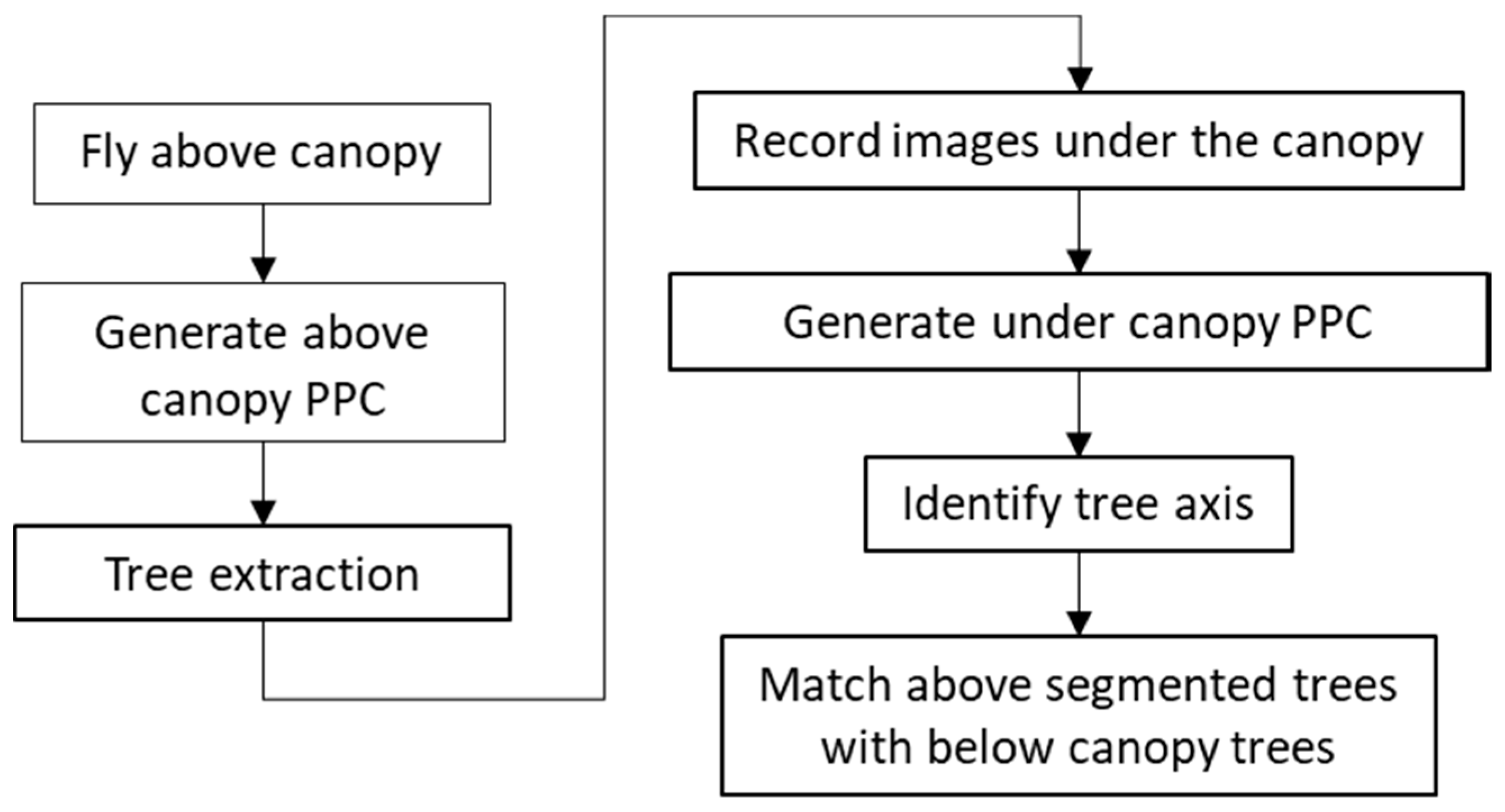
Figure 1. The procedure for geo-referencing trees from no to low accuracy georeferenced images acquired below canopy.
Remotesensing 11 01877 g001
Figure 2. Study area: (a) General location. (b) A perspective image inside the stand. (c) Nadir view of the point cloud.
Remotesensing 11 01877 g002
Figure 3. (a) Raw image captured with the Sigma EX 10 mm Fisheye lens mounted on the Nikon D3200 camera used to generate the below canopy point cloud. (b) Nadir view of the aligned and merged tie points build from three locations along a path where images where captured; the blue rectangles are the relative position of the sensor, the orange is the position of the above image, and the black lines shows the direction faced by the sensor (outward).
Remotesensing 11 01877 g003
Figure 4. Georeferenced possible trees estimated with TrEx from the above canopy point cloud (red stars). The background image is the orthophoto, which does not necessarily align with the point cloud.
Remotesensing 11 01877 g004
Figure 5. Correction to nadir view of the photogrammetric point clouds (PPC) produced with structure-from-motion at three locations (a) initial rendered position (almost perspective view); (b) oblique view; (c) nadir view.
Remotesensing 11 01877 g005
Figure 6. Preparing the PPC for estimation of the relative position of the trees shown at nadir in Figure 6. (a) perspective view of the raw PPC, (b) filtered PPC (points that are not mainly green or blue).
Remotesensing 11 01877 g006
Figure 7. Estimation of the relative location of the stems from the point clouds from Figure 6. (a) number of points from the filtered PPC, (b) relative location of the trees.
Remotesensing 11 01877 g007
Figure 8. The 50 m grid with their corresponding ID used to georeference all the trees. The yellow starts are the 641 trees extracted from above, the red dots represent the georeferenced trees segmented from georeferenced images.
Remotesensing 11 01877 g008
Figure 9. Impact of stem misalignment on the accuracy of tree matching for the five grid-cells used in geo-referencing all the trees; (a) 70% of the trees are found in the above and below tree segmentations; (b) 80% of the trees are found in the above and below tree segmentations.
Remotesensing 11 01877 g009
Table 1. Accuracy of tree matching for the 2500 m2 grid cells used for geo-referencing all the trees created from trees segmented using above canopy PPC.
Grid Cell# Trees Inside 2500 m2 Cell#Trees from GoPro Images Inside 900 m2 CellAccuracy [m]#Trees from Nikon Images Inside 900 m2 CellAccuracy [m]
82481.0671.08
112181.0190.98
172171.1281.05
222481.1171.15
3227111.0591.10
Accuracy--1.07-1.07