1. Introduction
Drought is one of the world’s most costly and widespread natural hazards, impacting water resources, agricultural production, ecosystems, human health, and the global economy [
1,
2,
3,
4]. Drought events are projected to be more intense and frequent for many regions of the world under global warming, placing further pressure on agricultural systems and natural resources, due to increasing demands from an ever-increasing global population [
5]. Semiarid regions such as Australia’s Murray-Darling River Basin, South Africa, and the America’s Middle West with vegetation cover face a greater threat from drought, especially agricultural regions because of insufficient rainfall, water management, and vulnerable vegetation [
6,
7,
8]. Throughout global history, extreme droughts have wreaked havoc on the agricultural systems in these semi-arid regions. Hence, understanding the vegetative response to drought in drought-prone, semiarid regions has drawn attention from meteorologists, ecologists, and agricultural scientists [
9,
10].
Droughts are often considered to have four major types: Meteorological, agricultural, hydrological and socioeconomic drought [
11]. The key that differentiates these different types of drought is time scale of dryness: Meteorological drought comes first with water deficits caused by high temperatures and low precipitation. After continuous meteorological drought, crops suffer from water deficits, and agricultural drought occurs. Among the four types of drought, agriculture is affected most directly and seriously by meteorological drought, and it is more difficult to understand than the others, because of the complication of interaction between vegetation and climate. To better understand drought effects, the construction of a drought monitoring index is the first step. Over the past decades, much effort has been devoted to drought monitoring, and a series of drought indices have been developed, such as water balance-based indices (Palmer Drought Severity Index (PDSI), Standardized Precipitation Index (SPI), Standardized Precipitation-Evapotranspiration Index (SPEI)) [
12,
13,
14], blended indices (U.S. Drought Monitor Index (USDM), Vegetation Drought Response Index (VegDRI)) [
15], indices constructed by joint distribution models (Joint Drought Index (JDI), Multivariate Standardized Drought Index (MSDI) [
16,
17] and other vegetation drought indices (Normalized Difference Drought Index (NDDI)) [
18,
19]. However, there is no single drought index that can reflect the situation across different regions and time scales, because the mechanism of drought and its effects vary considerably [
20]. To date, as a simple calculation using commonly available precipitation data, the traditional Standardized Precipitation Index (SPI) is widely used as a drought indicator, since it can be calculated at multiple time scales and adapted to different climates and drought types [
21,
22,
23].
To analyze the impact of drought on vegetation ecosystems, capturing the anomaly state of vegetation is of great significance. Many vegetation indices (VIs) have been developed to monitor vegetation conditions over large spatial ranges, such as the Normalized Difference Vegetation Index (NDVI) [
24], enhanced vegetation index (EVI) [
25], and ratio vegetation index (RVI) [
26]. NDVI has been proven useful for meaningful comparisons of seasonal and interannual changes in vegetation growth and activity, and it has been widely used in related studies to reflect the vegetation response to drought [
27,
28,
29,
30,
31,
32,
33,
34]. However, anomalies of growing seasons highlighted by the NDVI profile over the years can be attributed to several reasons, not only to extreme weather events like droughts, but also to agricultural practice; i.e., crop rotations or different planting times (winter crops versus summer crops). Therefore, more accurate methods are needed to characterize the abnormal state of vegetation influenced by drought. Dynamic time warping (DTW) [
31] is a match algorithm according to the warping similarity of temporal profiles, and it is proven to be an efficient solution to handle these issues in crop classification, effectively reducing the intra-class variations related to different vegetation types and agricultural and land management practices [
35,
36,
37]. But to date, the effect of this method on vegetation anomaly calculations has not been well evaluated in related studies.
The main challenge for monitoring the response of vegetation to drought with satellite imaging is the analysis of the relationship between vegetation and drought, as well as the calculation of the vegetation response’s time lag. The effect of drought on vegetation is cumulative and nonlinear, and it is not manifested by vegetation at a certain degree or time during the year [
38,
39,
40]. Several factors determine vegetation response, including various drought characteristics (duration, severity and intensity), vegetation characteristics and phenology, and the general environment conditions of the location (e.g., soil type and elevation) [
41,
42,
43]. This complexity and nonlinearity make it more difficult to extract lag time relationship between climatic conditions and vegetation response. The correlation coefficients and regression method were widely used in most previous studies to analyze the relationship of NDVI and SPI, and over an approximately 1–3 month scale, a strong correlation between NDVI and SPI have been proven [
44,
45,
46,
47,
48]. However, more detailed time lag information observed by satellite images is still not clear. At present, research on the large-area response lag of remote sensing-derived variables, such as VIs have mainly been conducted on a monthly scale and have not explored in finer time scales. In addition, few previous studies have concentrated on the relation between vegetation anomaly and drought, since the vegetation index, rather than ‘vegetation anomaly’ index was used to analyze the relationship between vegetation and drought, it is difficult to remove the influence of non-drought factors (seasonal change and vegetation growth) on the changes of a vegetation index [
44,
49]. Some studies have used standard scores to characterize the anomalies of vegetation and rainfall, and other methods have been tried to calculate the time lag of vegetation’s response to drought in more sophisticated way [
50,
51,
52]. More detailed study of vegetation response to drought is needed to give a more accurate response relationship and response time lag.
The overall objective of this study is to develop a refined methodology to map and characterize spatial-temporal dynamics of detailed vegetation response lag to drought in semiarid regions, focusing on Nebraska. Daily time series of MODIS NDVI data and the Daymet dataset over a 15-year study period (2000 to 2015) were used to create annual maps of vegetation response lag, and assess the variations of lag among different vegetation types. In addition, we analyzed the potential contributors to vegetation stress using random forest.
2. Materials and Methods
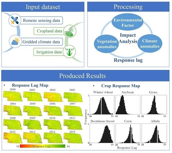
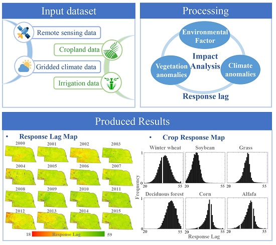
The MOD09GQ time-series, Cropland Data Layer (CDL) and Daymet dataset from 2000 to 2015 were used to extract the vegetation anomaly, and climate anomaly, respectively. The irrigation data and DEM were also applied to the driving force analysis of vegetation response diversity. The methodological workflow consisted of the following steps (
Figure 1): (1) Data preprocessing and NDVI time-series smoothing; (2) calculation of SPI (precipitation anomaly); (3) calculation of the temperature anomaly; (4) calculation of the vegetation anomaly, which involves the extraction of average phenology NDVI profile, DTW match of NDVI observed time-series and phenology profile, and the anomaly calculation of NDVI at daily scale; and (5) extraction of vegetation response lag based on lag correlation coefficient.
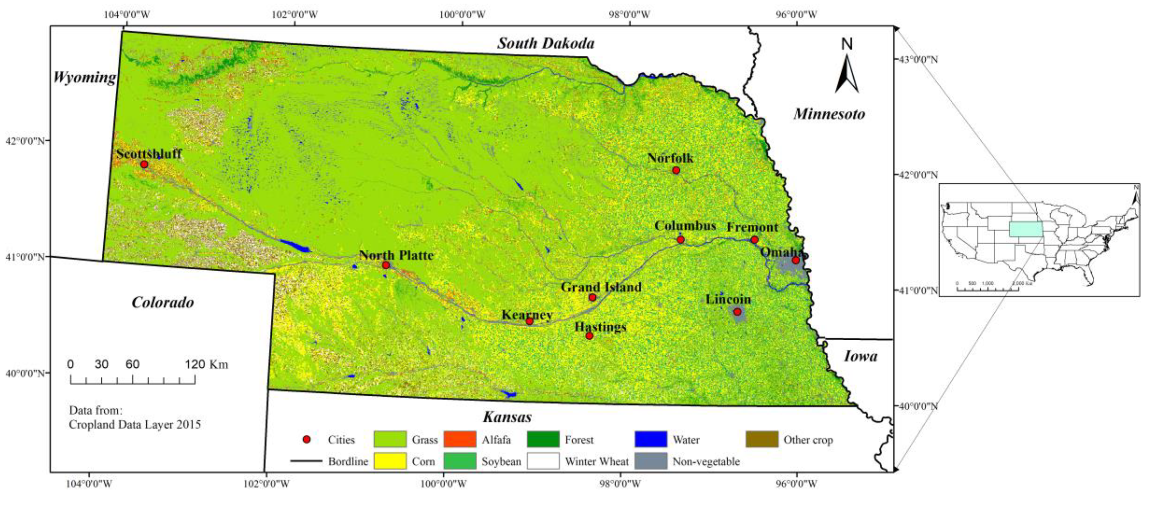
Nebraska is located approximately between 40° and 43° N latitude and 95° and 104° W longitude, with a total area of 200,365 km
2. The state is located in the U.S. Central Great Plains region, and is an agriculturally dominated state supporting both irrigated and rainfed crops. The western and central parts of Nebraska are covered by expansive grasslands, which is a natural vegetation ecosystem that is less affected by human activities, both irrigated (e.g., alfalfa, corn, and soybeans) and rainfed, dryland crops (e.g., winter wheat). The eastern part of Nebraska is extensively cropped in a primarily corn-soybean cropping system under rainfed production. Nebraska ranks among the leading producers among states in the U.S. for the state’s main crop types of corn, soybean, winter wheat, and alfalfa (
Figure 2).
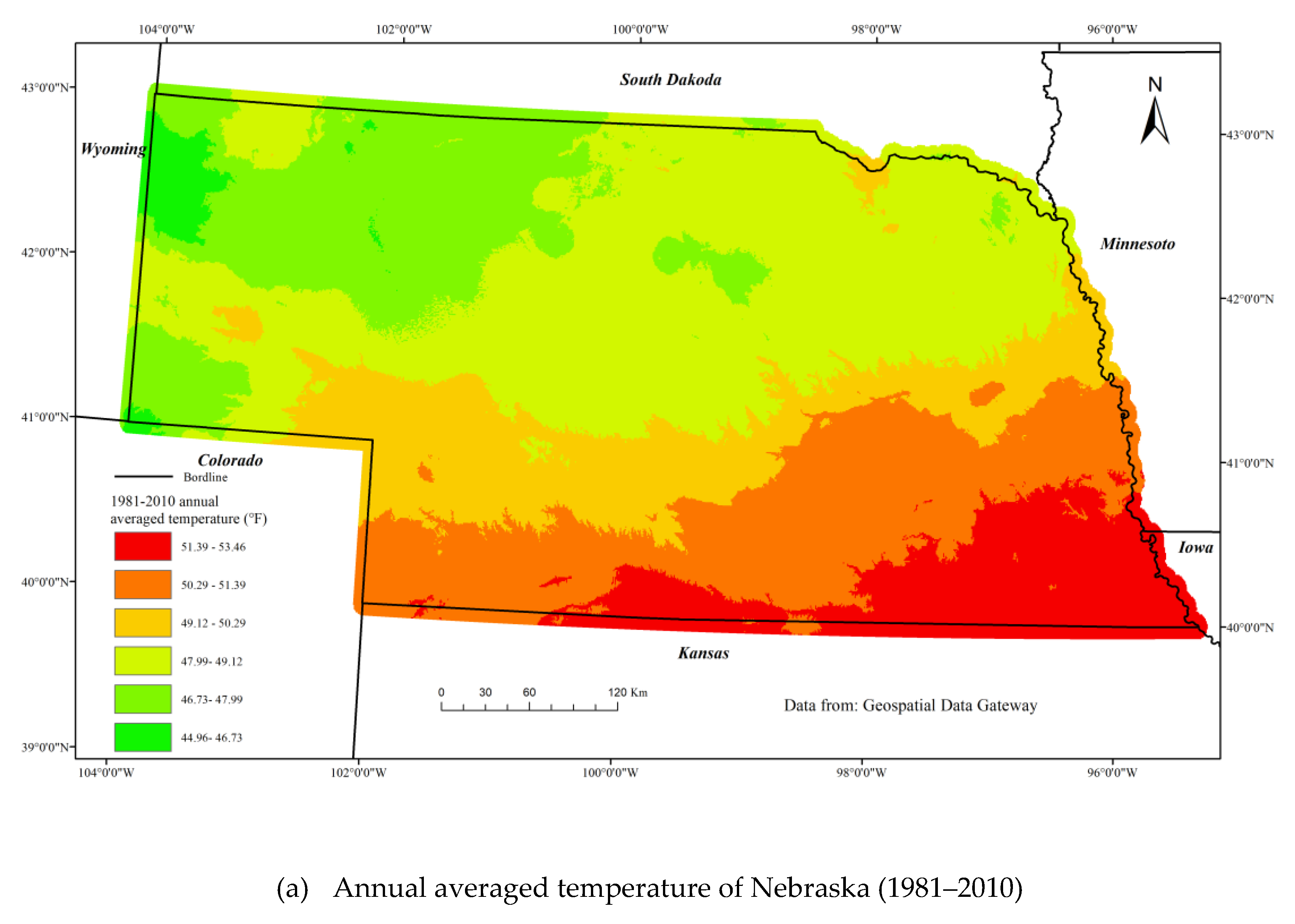
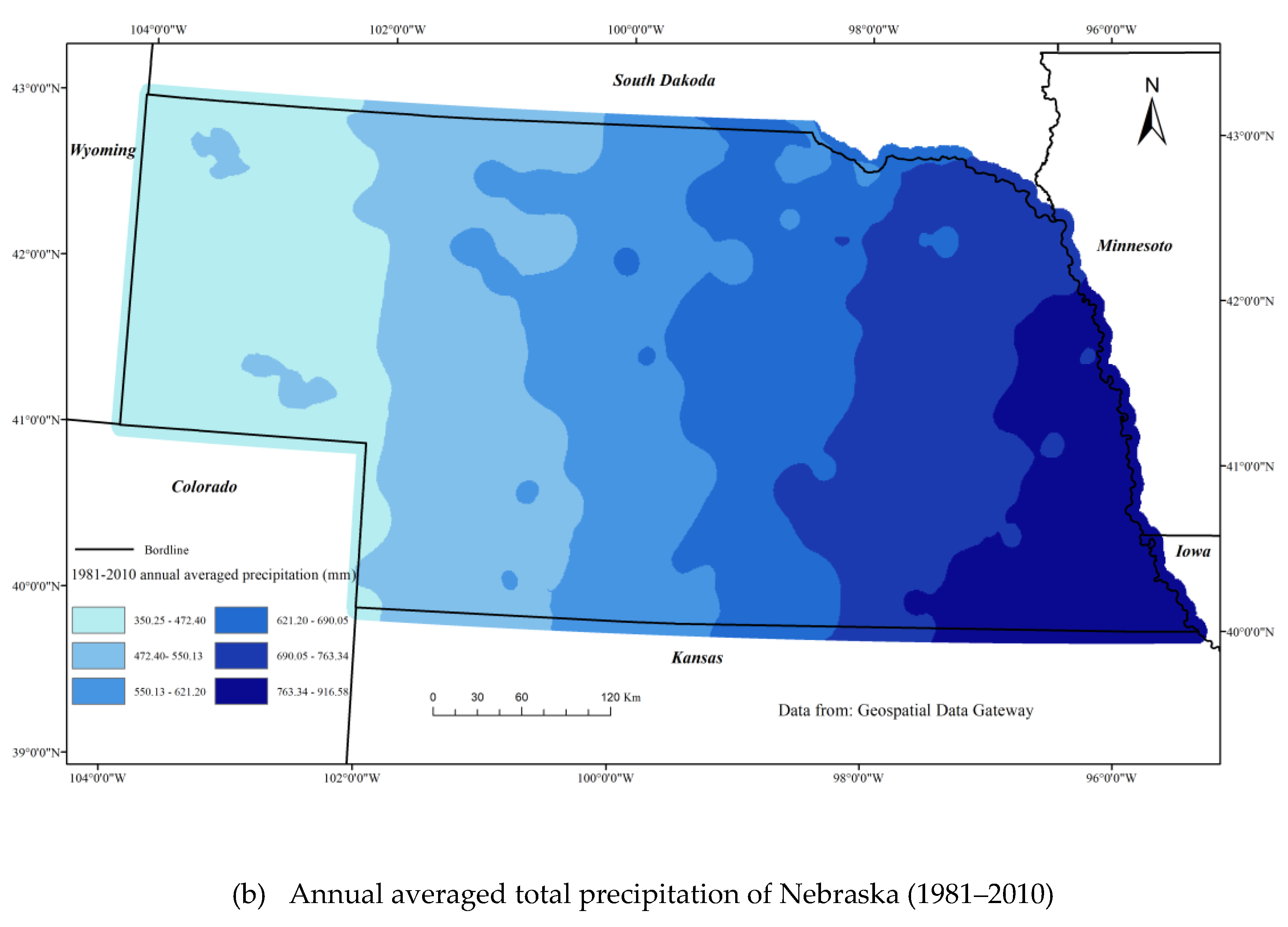
Nebraska has two major climate zones: Continental in the east and semiarid in the west. The state has a steep precipitation gradient ranging from about 380 mm in the west to >800 mm in the east (
Figure 3b). The temperature in the south is higher than that in the north (
Figure 3a) (
https://datagateway.nrcs.usda.gov/GDGHome.aspx). These precipitation and temperature gradients reflected in the spatial distribution of cropping types, agricultural management practices, and vegetation types across the state. A combination of dryland, irrigated crops, and short grass prairie is predominate in the west, transitioning to predominately rainfed corn-soybean systems and tall grass prairie vegetation types in the east. Rainfall fluctuates greatly throughout the year and across the spatial extent of the state, and also has a high level of inter-annual variability in precipitation, resulting in periodic drought events [
53].
Nebraska has been profoundly affected by long and extreme droughts for centuries. In recent years, global climate change has significantly increased the frequency and intensity of extreme weather events in Nebraska [
55]. For example, the severe flooding in 2011, and extreme drought in 2012, which was the driest and warmest year on Nebraska’s record [
56].
2.1. Data and Preprocessing
The MODIS time-series, Cropland Data Layer, and Daymet dataset from 2000 to 2015 were used to extract the vegetation anomalies and climate anomalies respectively. The irrigation data and Digital Elevation Model (DEM) were applied for the driving force analysis of vegetation response diversity. All the spatial data were resampled to 250 m spatial resolution for further data processing.
2.1.1. Time-series MODIS Data
The NASA MODIS sensor offers timely and large-area surface monitoring observations with high temporal (near daily) and moderate spatial (250 meter) resolutions. MODIS data sets products were acquired from NASA [
57] (
https://modis.gsfc.nasa.gov/) with the image data products calibrated and atmospherically corrected for gases, aerosols, and cirrus-cloud effects using the MODIS atmospheric correction algorithm [
58,
59]. In this study, MOD09GQ daily products from 2000 to 2015 were used to calculate the NDVI time series data [
60].
MOD09 red and near-infrared (NIR) reflectance imagery, centered at 645-nanometer and 858.5-nanometer wavelengths, respectively, are available at 250-m resolution from the MOD09GQ product on a daily time step. This MODIS image data product has scientific quality assurance (QA) flags describing the overall image data quality, band-specific quality, atmospheric correction state and adjacency correction state that was used to reduce the noise of NDVI time series data during time-series NDVI reconstruction in this study.
Three MODIS images (h10v04, h10v05, h11v04) were joined with the MODIS Reprojection Tool (MRT) [
61,
62] to cover Nebraska, and the Land Data Operational Products Evaluation (LDOPE) tool [
63] (
https://lpdaac.usgs.gov/tools/ldope/) was applied to parse and interpret the QA Science Dataset (SDS) layers. The ‘unpach_sds_bits’ tool and the ‘cp_proj_param tool’ of LDOPE were used to decode the MOD09GQ quality control band. The decoded QA band represents that the quality of every pixel in every daily image would be used in a data smoothing procedure to help remove the influence of anomaly data.
The reflectance data of the red and NIR bands were used to calculate the NDVI as an indicator of the photosynthetic capacity of the vegetation at the pixel level. The NDVI was calculated using Equation (1):
where
ρNIR (846-876 nm) and
ρRED (620–670 nm) are the bidirectional surface reflectance for the MODIS bands.
2.1.2. Time Series Smoothing
The study area can experience periodic cloud cover throughout the growing season, which seriously affects the quality of the NDVI time series. Considering our purpose is to find vegetation response to climate change in remote sensing time series, which represents anomaly fluctuation in temporal profile, the quality of NDVI time series is a critical issue, since cloud cover could cause a similar anomaly. To reduce the noise of NDVI time-series, the Savitzky-Golay filter [
64] was applied for its simplicity and reliability.
The Savitzky-Golay filter is a simplified least squares-fit convolution for smoothing and computing derivatives of a set of consecutive values (a spectrum) [
64]. It was proven to be the most efficient algorithm for separating distinct multi-temporal profiles, compared with other common smoothing algorithms [
65]. Furthermore, it effectively preserve key temporal features, such as the relative maximum, minimum, and width of the time-series dataset [
66,
67].
To achieve better filtering, data quality control flags, assigning corresponding weights were used to identify spurious observations for the SG filter. Quality control flags were calculated using LDOPE and ArcGIS. The CMD batch program of the LDOPE tool was used to decode the quality information of the red and NIR bands in batches (
Table 1), and ArcGIS was used for batch grading synthesis (
Table 2) to obtain the quality grade file corresponding to NDVI. Subsequently, the SG filter was applied by setting a window width of four, one envelope iteration, and an adaptation strength of two. Fitting iterations of the SG filter were set to two. The weight of quality level one was one; the weight of quality level two was 0.5, and the weight of quality levels three and four was set as zero to remove the image noise. After the S-G filtering, the noises of quality level three images were completely removed, and the noises of quality level two images were obviously improved.
2.1.3. Daymet Dataset
The meteorological data were downloaded from the ORNL DAAC (
https://daymet.ornl.gov/). The Daymet data set provides gridded estimations of weather variable for North America with daily time resolution and 1-km
2 spatial resolution [
68]. The daily mean temperature dataset (2000–2015) and daily total precipitation dataset (1981–2015) were used in this study, and were first resampled to 250 m by the bilinear interpolation resample method. The daily mean temperature data were processed by temperature anomaly calculation, and the daily total precipitation data were used to acquire the Standardized Precipitation Index (SPI) in Nebraska since 1981.
2.1.4. Cropland Data Layer
The Cropland Data Layer (CDL) [
69], hosted on CropScape (
https://nassgeodata.gmu.edu/CropScape/), provides a raster, geo-referenced, crop-specific land cover map at 30-m spatial resolution for the continental United States. The crop distribution map from 2000 to 2015 were resampled to 250 m by the majority resample method, and used to calculate accurate vegetation anomaly. In addition, the crop distribution in 2012 was applied to assess crop-related vegetation response to drought.
2.1.5. Irrigation Data
The MODIS Irrigated Agricultural Dataset (MIrAD) [
70] provided by the U.S. Geological Survey (
https://earlywarning.usgs.gov/USirrigation) was used as the irrigation data source. This data set was derived using a land cover data set, USDA agricultural irrigation area statistics and the annual maximum VI information calculated from MODIS VI data. The MirAD has a nominal spatial resolution of 250 m and irrigation distribution in 2012 was available to analyze the human effect on extreme drought in Nebraska.
2.1.6. Digital Elevation Model (DEM)
The ASTER Global Digital Elevation Model (ASTGTM) provided by NASA (
https://earthdata.nasa.gov/) was used as a Digital Elevation Model (DEM) in this study. The spatial resolution of this product is 30-m and was resampled as identical resolution (250-m) of MODIS by bilinear interpolation resample method. The DEM influences the natural environment of vegetation (local temperature and rainfall event), thus it was applied to analyze the driving force of various vegetation response to drought.
2.2. Methodology
The methodological workflow consisted of the following steps (
Figure 2): (1) Data preprocessing and NDVI time-series smoothing (see
Section 2.1.2); (2) calculation of SPI (precipitation anomaly); (3) calculation of the temperature anomaly; (4) calculation of the vegetation anomaly, which involves the extraction of average phenology NDVI profile, DTW match of NDVI observed time-series and phenology profile, and the anomaly calculation of NDVI on a daily scale; and (5) extraction of vegetation response lag based on lag’s correlation coefficient.
2.2.1. Standardized Precipitation Index (SPI)
To better capture the spatial patterns and temporal variations of dryness, the Standardized Precipitation Index (SPI) [
14] was adopted in this study as the drought index. Compared to other drought indices, the SPI has several advantages, including unambiguous theoretical development, robustness, versatility, including temporal flexibility, and the simplicity of requiring only a precipitation data input [
71,
72].
SPI has different scales for different application. One-month SPI could reflect the soil condition, which directly influences the vegetation growth. In our study, one-month SPI was applied both for reflecting annual drought events and calculating accurate response lag. To be specific, we first calculate the annual average of one-month SPI in 2000–2015 to select normal climate year and relatively severe drought year for further study. Then, for the severe drought year, in order to better find the accurate temporal scale of vegetation response, we calculates the one-month SPI, but represented it on daily scale with a one day time step, in accordance with daily scale of NDVI time-series. For each day, we calculated the cumulative rainfall for the previous 30 days to calculate a one-month scale SPI (Equation (2)). Finally we computed 30 times the one-month SPI, since there are approximately 30 days in a month.
where
Pi denotes the daily precipitation at day
i,
d represents the previous
d day, and
Psum represents a 1-month scale cumulative precipitation at day
i.
According to the World Meteorological Organization, at least 20–30 year precipitation record should be used to calculate the accurate SPI [
73,
74]. In this study, a 35-year historical record of precipitation data (1980–2015) were used to assure the SPI accuracy. For a more detailed explanation of the theory and calculation of SPI, one may refer to these related studies [
14,
75,
76].
2.2.2. Temperature Anomaly
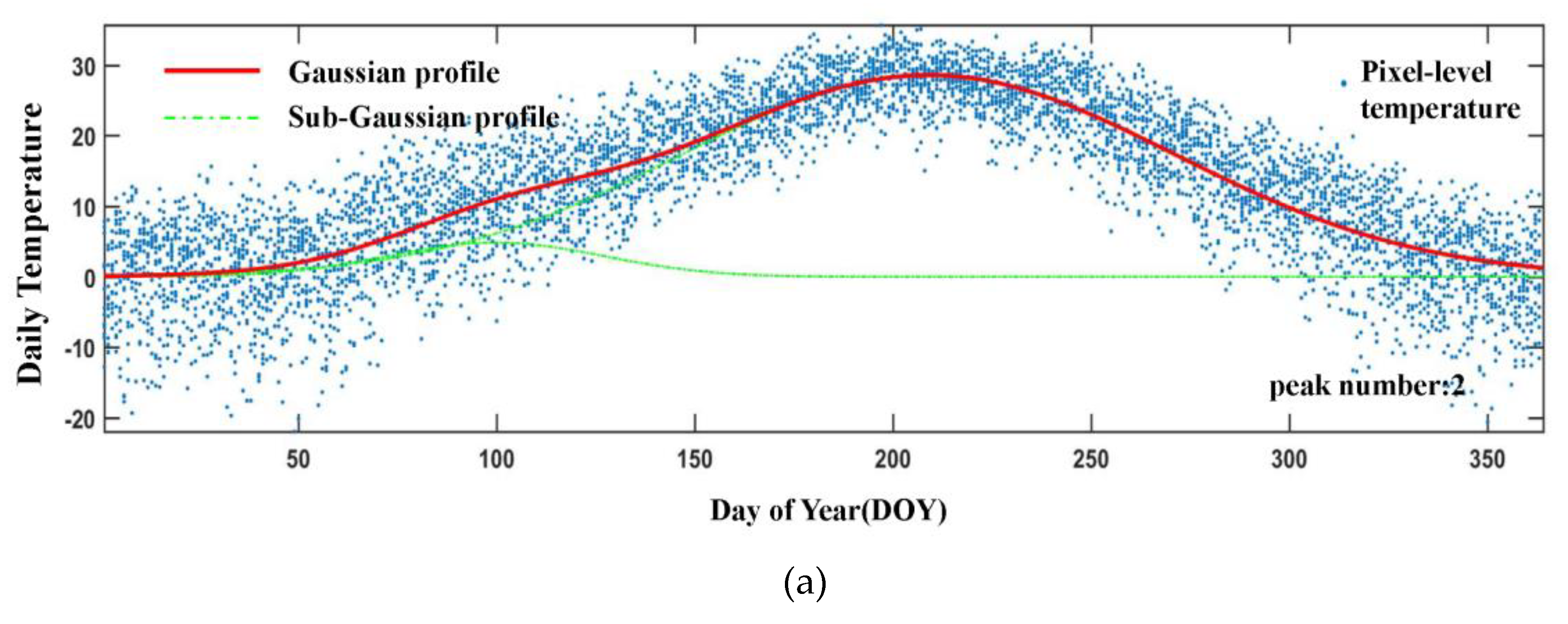
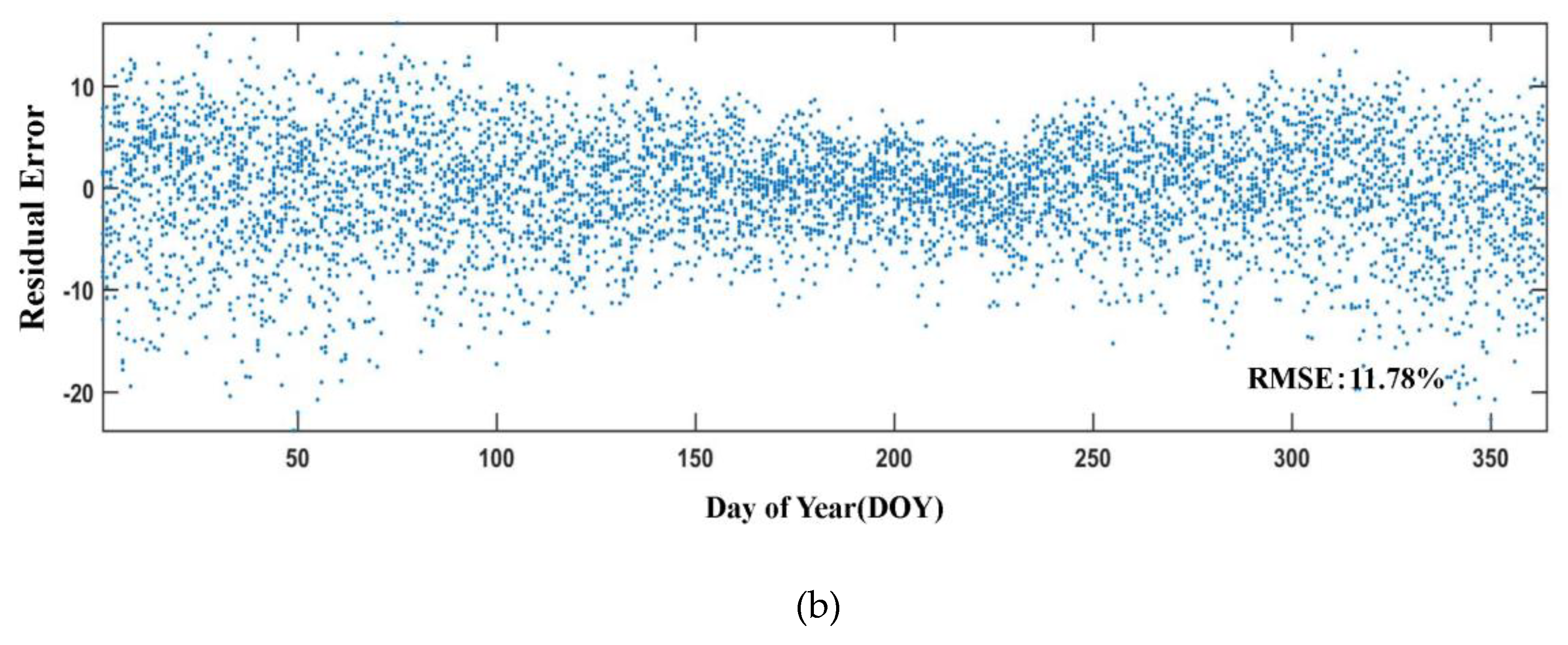
The difference between the observed value and the multiyear Gaussian fitting value is used as the index of the temperature anomaly (Equation (3)). The distribution of daily mean temperature in a year is similar to Gaussian distribution; therefore, the normal daily mean temperature could be obtained by Gaussian fitting numerical values (
Figure 4a). Gaussian fitting values for characterization of normal daily mean temperature compared to the traditional average characterization method have higher reliability and can effectively eliminate the interference of abnormal climate. Considering that the temperature across two climatic zones in Nebraska has obvious spatial heterogeneity, the Gaussian fitting and the calculation of temperature observation are processed at pixel level. We conducted many tests, and found out that lots of pixels have a small temperature peak in spring, and the double Gaussian model outperformed the single Gaussian model. Thus, a double Gaussian model was used to fit the normal daily mean temperature, because of its better accuracy (
Figure 4b).
where
t is the day of year (DOY),
Tanot is the temperature anomaly at date
t,
Tt denotes the observed daily mean temperature and
denotes the multi-year gaussian fitting value (normal temperature) at date
t.
2.2.3. Vegetation Anomaly
Vegetation anomaly calculations include three steps: (1) Derivation of the phenological NDVI profile of vegetation, (2) dynamic time warping (DTW) of the NDVI time-series and phenological NDVI profile, and (3) vegetation anomaly calculation.
The first step in calculating the vegetation anomaly is to calculate the NDVI phenology curve of each vegetation type. Based on temperature anomaly and multi-year SPI in Nebraska, the period from 2008 to 2011 were selected as ‘normal’ climate years without extreme climatic events. Using crop information from the CDL, the phenological NDVI profile of each vegetation type was then obtained by averaging the daily NDVI values for all pixels by vegetation categories. These phenological NDVI curves represent the growth of each vegetation type under mean climate conditions.
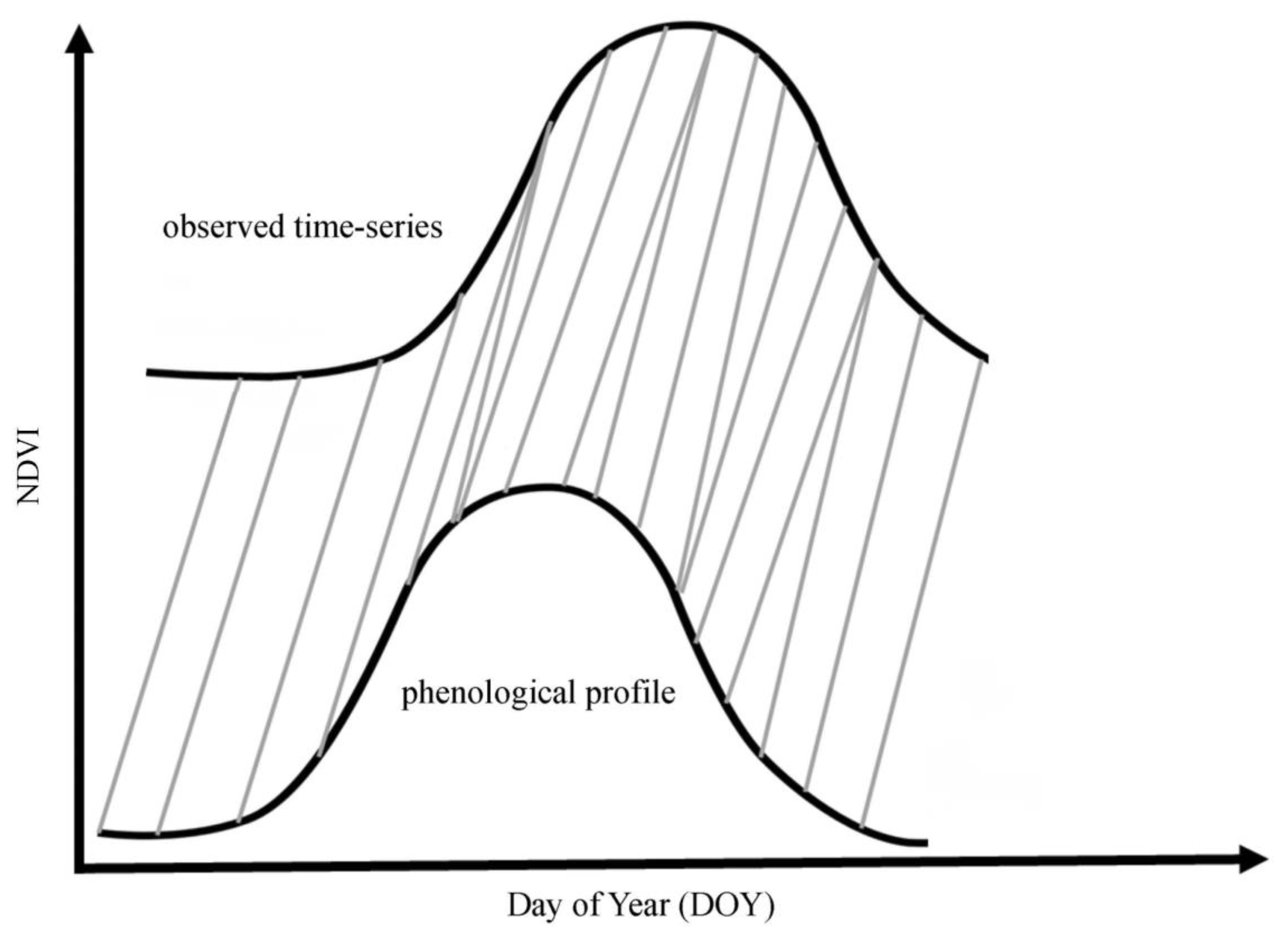
The second step is the calculation of vegetation anomaly using DTW match algorithm. It is important for reducing the false anomalies caused by the different planting and harvesting periods. DTW is an algorithm that uses dynamic programming to modify time-series data sequences to find the minimum bending distance between two time sequences to achieve sequence matching [
77]. DTW has three constraint rules: Monotonicity constraint, endpoint constraint, and continuity constraint. Under these constraint conditions, the bending path is obtained by minimizing the sum of path distance.
Note that the direct use of DTW makes any real anomaly disappear, because the small fluctuation of the anomaly on the daily scale would also be weakened by DTW. Therefore, the Gaussian filter was first applied to reconstruct the time-series NDVI data sequence before the DTW was applied to remove small fluctuations. The DTW was then applied to the Gaussian-filtered NDVI curve to obtain the matching date (
Figure 5). The original curve is then matched according to the matching date. Finally, vegetation outliers were calculated according to Equation (4):
where
is the vegetation anomaly value of pixel
i in day
t,
denotes the NDVI of pixel
i in day
t,
k is the crop type of current pixel
i, and
is the normal NDVI value of crop type
k in matched day
.
During the non-growing season period, the fluctuation of the NDVI profile is not a manifestation of crop growth anomalies, but is more likely to be caused by soil, wild grass, and noise of the remote sensing image. Therefore, when the NDVI anomalies were calculated using DTW matching, the planting date and harvesting date were obtained according to the match date of the start and end of the growing season. The NDVI anomalies before and after planting were filled with ‘NaN’ to obtain the final vegetation anomaly data.
2.2.4. Response Lag
The lag period is the key to investigating the response of vegetation to climate anomalies. It is also the most challenging and key point in obtaining accurate correlation and function relations in climate-vegetation response comparisons. Due to its simple principles and wide application, the lag correlation coefficient was applied to analyze the data time series and determine the lag period according to the highest correlation coefficient.
Considering that the temporal anomaly and precipitation anomaly have different response mechanisms, the vegetation response lag to temperature anomalies and rainfall anomalies were extracted respectively.
The response of plants to climate anomalies is characterized by accumulation and hysteresis. In this study, we defined the ‘response’ period and ‘lag’ period. The ‘response’ period refers to the accumulation of climate anomalies that influence vegetation, and the ‘lag’ period represents the lag time of the vegetation response. In this study, response lag was calculated as the sum of the response and lag periods.
Temperature anomaly was calculated in daily scale, so we first calculated the sum of temperature anomaly on a different scale (one week–two months) which represents the ‘response’ period. Then the lag correlation coefficients were computed to get the optimal ‘lag’ period on each ‘response’ scale. Finally, based on the different optimal lag correlation coefficient on different ‘response’ scales, the optimal ‘response’ scale was decided by the maximum correlation coefficients, and response lag was obtained by the sum of ‘response’ period and ‘lag’ period. As for precipitation response, since we calculated SPI on a one-month scale, it was hard to define the ‘response’ period and ‘lag’ period, so the response lag was totally decided by the results of maximum lag correlation coefficient. In order to catch the drought response in climate anomaly year, we shrank the input time-series of lag correlation calculation by setting the climate threshold value (SPI < 1, temperature anomaly > 1) and maintained a certain duration (duration > 50 days).
2.2.5. Random Forest
Random forest (RF) [
78] is an ensemble learning method of cart trees to analyze nonlinearity and interactions between predictors [
79]. The main advantages of RF include significantly reducing possible overfitting [
80], and minimizing influence by collinearity among analysis variables [
81], but up to now this method is not common in climate and hydrological science. In this paper, RF was used to understand what or how factors contributed to vegetation anomalies. More specifically, it was applied to analyze the relationship between vegetation anomalies and a series of factors (climate anomalies, irrigation, crop type, growth period, DEM and image quality).
The RF model was run using the TreeBagger class on matlab2014b at the pixel-level. Two parameters need to be tuned for RF, namely the ’NumTrees’, which is be created by randomly selecting samples from the training samples, and ’MinLeafLeaf’, which is the minimum number of observations of per tree leaf. The ‘MinLeafLeaf’ is set up as five according to multiple experiments, and the ‘NumTrees’ parameter was set up as 500 according to the ‘out-of-bag squared error,’ and the out-of-bag error of our model eventually reached below 0.0015, which means a high accuracy and good generalization. The importance for each predictor variable (feature) was also analyzed in our study. The factor importance index is the increase in prediction error if the values of that variable are permuted across the out-of-bag observations. This measure is computed for every tree, then averaged over the entire ensemble and divided by the standard deviation over the entire ensemble.
3. Results and Discussion
3.1. Spatial-temporal Pattern of Drought
Spatial and temporal patterns of drought are useful for revealing the occurrence patterns of climatic and vegetation anomalies in the study area. The consistency of spatial and temporal patterns of climatic and vegetation anomalies is very important in investigating the correlation between climatic-vegetation interactions over the study area.
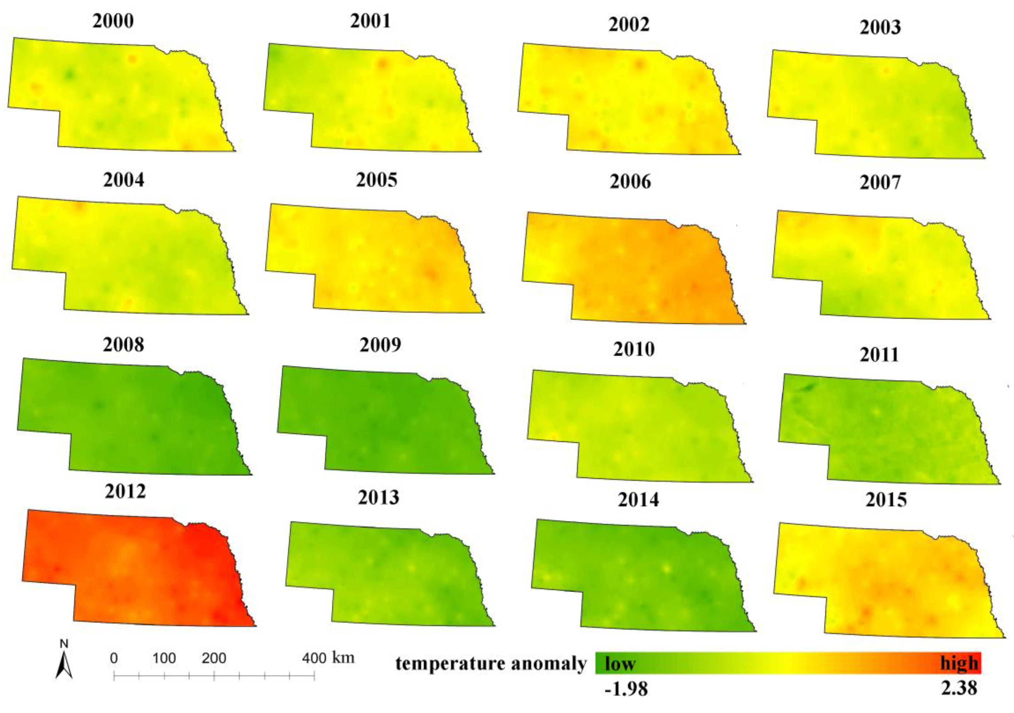
Figure 6 shows the spatial pattern of temperature anomalies from 2000 to 2015 in Nebraska. In 2012, Nebraska had extremely high temperature across the whole state, and in 2005, 2006 and 2015, heat waves also swept through Nebraska. Abnormally high temperatures generally occurred uniformly in spatial pattern. During the periods of 2008 to 2011 and 2013 to 2014, the temperature was relatively cool for the state.
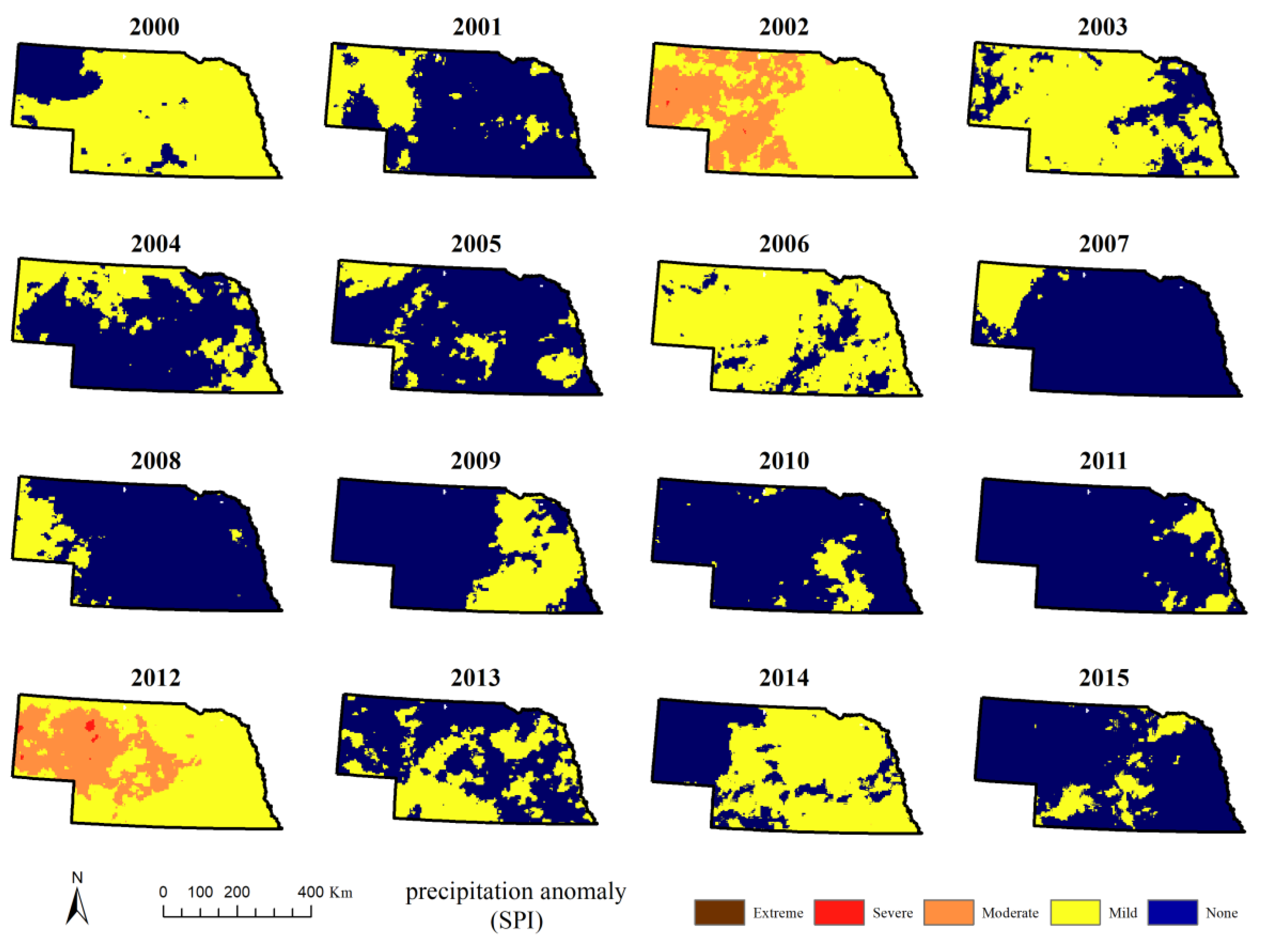
Annual averaged one-month SPI is more conducive to the demonstration of precipitation anomalies that influence vegetation. Based on the spatial-temporal pattern of annual averaged SPI, as shown in
Figure 7, it can be clearly seen that severe drought events impacted the entire state of Nebraska in 2002 and 2012, which was consistent with the findings of the U.S. Drought Service’s seven-day drought observation with the USDM Index (
Figure 8). USDM is based on six key indicators (Palmer Drought Index, SPI, Keetch-Byram Drought Index, modeled soil moisture, seven-day average streamflow, and precipitation anomalies), numerous supplementary indicators, and local reports from many expert observers (
http://droughtmonitor.unl.edu/) [
82]. However, the duration and severity of drought detected by SPI1 and USDM showed a different pattern. The 2002–2003 and 2012–2013 were detected by USDM as severe drought events, but as for one-month SPI, only 2002 and 2012 were severe years, at which times droughts were detected earlier than USDM. Considering vegetation is first influenced by meteorological drought, SPIs were more suitable than USDMs for vegetation drought monitoring. In our results, Nebraska experienced widespread mild droughts in 2000, 2003, 2006 and 2014. Compared with temperature anomalies, the spatial pattern of rainfall anomalies has a higher degree of fragmentation and spatial heterogeneity due to several factors (e.g., the atmospheric circulation, and the morphology of the territory). The occurrence of rainfall anomalies does not show an obvious drought-prone spatial sub-region: In 2000, a separate humid region appeared in the northwest corner of Nebraska, but in 2007, this region was drier than other area in Nebraska. Similarly, the drought in 2003 occurred in the central part of Nebraska, but the drought in 2010 mainly occurred in northwestern Nebraska, and in 2014, drought hit southeastern Nebraska. The occurrence of scarce rainfall has extremely complex spatial rules, and it is dependent on local spatial effects, which is difficult to include in the module. Therefore, precipitation anomalies are difficult to spatially predict.
Discernible significant positive coherence can be observed when comparing temperature (
Figure 6) and precipitation (
Figure 7) anomalies. Higher temperatures occurred frequently with scarce precipitation. Notably, this correlation is more pronounced under extreme weather conditions than for normal climate anomalies. For example, in 2002 and 2012, both severe temperature anomalies and scarce precipitation occurred throughout Nebraska. However, in 2003 and 2014, dryness was not associated with high temperature, and in 2005 and 2015, higher temperature was not associated with dryness.
3.2. Driving Force Analysis
The random forest method helped us to understand the contributors of vegetation anomalies among many factors (climate, irrigation, crop type, growth period, DEM, and image quality).
Figure 9 presents the factor ranking results. One-month SPI were most important factor to vegetation response, and crop type also decided the response lag. The daily temperature anomaly shows a relatively low influence on vegetation stress. Some studies have found the benefit of daily higher temperatures; however, heat waves (temperature above normal lasting from a few days to a few weeks) could damage vegetation [
28,
83]. Irrigation in many cropping systems of central and western Nebraska mitigates the effects of precipitation deficits by maintaining adequate soil moisture conditions through water application, unless under the most extreme of drought conditions, when irrigated crops are affected. The growth period also affects the extent of climatic influence on vegetation. DEM, image quality, and daily climate conditions are not important for vegetation condition responses in this study.
3.3. Spatial-temporal Pattern of Response Lag
In the analysis of the spatial-temporal heterogeneity of climatic and vegetation anomalies, it was found that the spatial-temporal scale of vegetation response was not consistent with that of temperature anomalies and rainfall anomalies, and the lag response relationship was not consistent. Therefore, the vegetation response lag to temperature anomalies and rainfall anomalies should be extracted separately. Spatial-temporal patterns of response lag are useful for revealing the cumulative effect of climate anomalies on vegetation conditions.
In this study, the cumulative temperature anomaly was found to have a low correlation with vegetation anomalies using the lag correlation coefficient, and no stable, specific lag period was found to have a high correlation with vegetation anomalies. The influence of high temperatures on vegetation is often a bi-directional, complex non-linear relationship. On one hand, an appropriately timed, high temperature can lead to increased photosynthesis and better conditions for vegetation, particularly during parts of the growing season where the energy environment is key to vegetation growth (e.g., spring green-up of the vegetated phase of plant growth). However, heat waves can cause stress, and damage vegetation (e.g., during reproductive phase of crops). This nonlinear relationship is difficult to characterize with a function, especially for the correlation of high temporal resolution time series like the NDVI profiles used in this study. In addition, there is a possibility that daily maximum temperature could have a better correlation with vegetation anomaly. Also, the single-Gaussian fitting of normal temperature using a more than 30-year time-series may improve the lag correlation results.
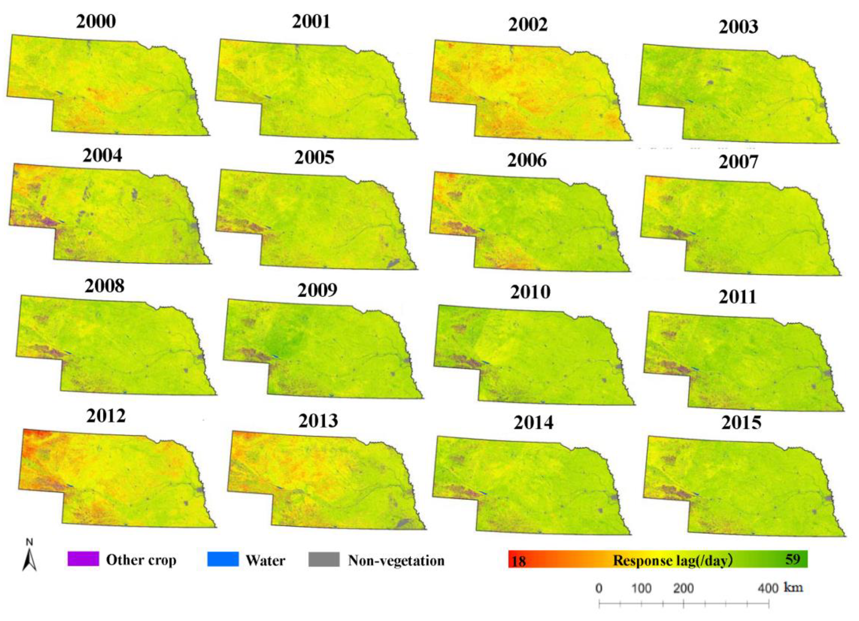
The response lag of vegetation to the one-month SPI is shown in
Figure 10. The lag period of drought ranged from two weeks to one and a half months; most lag periods were approximately 30–45 days. Under normal or wet climate conditions, vegetation did not perform an obvious response behavior, but its response along an accumulated rainfall deficit that follows a normal period was slower due to the water availability in the soil. During the two extreme drought anomaly years (2002 and 2012), vegetation responded rapidly to the deficit of accumulated rainfall. In 2013, the influence of the precipitation anomaly only covered the northwestern part of Nebraska; however, the SPI12 index (
Figure 5) is normal in this region, which means that the response lag and the vegetation’s condition were not only decided by the water shortage, high temperatures, and plant diseases may have accelerated vegetation response. Grassland is the predominant cover type in northwestern Nebraska, which indicates a stronger response of grassland compared to that of cropland, even when cropland is facing more severe drought conditions. A possible explanation is that crops of eastern part are irrigated (corn, in particular, is a crop with high water requirement) compared with wild grass. For this reason, yearly irrigation scheduling should be considered in order to compare different behaviors, especially during drier seasons.
In 2006, apart from grassland, there was a unique severe response region in the southwestern part of Nebraska. This area was largely planted with winter wheat, and the 2006 drought conditions occurred only in winter and spring of that year. Given that the primary growing season for winter wheat is spring and early summer with a mid-summer harvest period, the early-year drought conditions during the late winter and early spring of 2016 greatly reduced soil moisture conditions to support winter wheat production, resulting in widespread drought stress in wheat over this region. Therefore, vegetation damage and response lag were also determined by the time (season). However, under the extreme climate conditions (2002 and 2012), the response lag pattern was consistent with the SPI12 distribution; other reasons for this influence seem to be implied. As seen from the spatial pattern in the
Figure 7, the vegetation with a relatively fast response to precipitation deficit in the dry period is mainly concentrated in western Nebraska, which is less affected by human activities (irrigation, water conservation projects) and where the vegetation type is mainly grassland. This shows that human activities can mitigate some effects of climate stress, especially drought-induced water stress, on crops.
The results in this section show that the length of the lag period is related to the severity of climate anomalies to some extent. When severe precipitation deficits occur, vegetation in general has a shorter lag period for climate response, but the lag period of response is usually no less than two weeks, which may be due to the accumulated soil moisture and the protective stress mechanisms of vegetation. Besides, the results also implied the possibility to use an SPI1 with a moving window of one week instead of one day.
3.4. Crop Response Lag
Frequency distribution of response lag by vegetation categories can further characterize the diversity of vegetation response to climate. To better reveal the response lag of different vegetation types to climatic anomalies, we chose the most severe drought year (2012) for further analysis. A total of 1000 random pixels were selected for six main vegetation cover types according to the coverage area size that included: Grass, soybeans, winter wheat, corn, deciduous forest, and alfalfa. In order to reflect the real situation, random pixels were limited and adjusted according to the geographical location and satellite quality; the low quality of pixels in the remote sensing image is removed based on QA band.
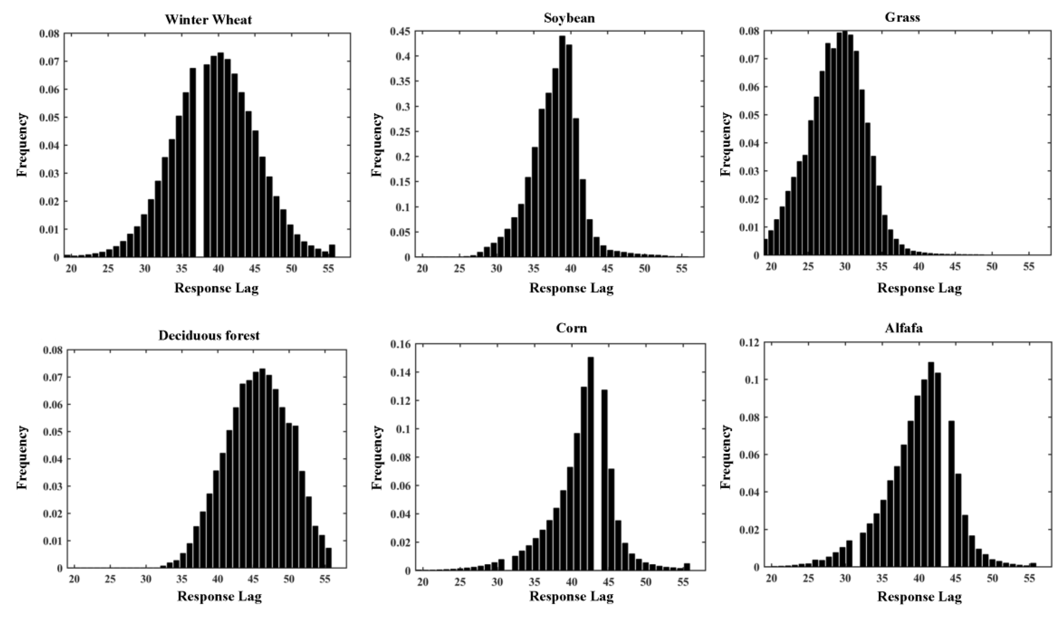
As
Figure 11 demonstrates, among all vegetation types, the response lag of grassland is the shortest, distributed mostly around 30 days and rarely exceeding 35 days. Considering its location in the western region of Nebraska where human activity is limited, grassland may suffer more serious effects from water deficit stress than the other crop-related vegetation types. Deciduous forest had the longest response lag of all vegetation types of up to 48 days, which means that when the deciduous forest faces an extreme climate, its own stress responses and adaptability make it less influenced by climate anomalies. Trees have a longer response lag to prolonged drought because of their deep root system.
For crops, the lag period of winter wheat had a large lag response range, spanning from 20 to 55 days. The growth period of winter wheat is different than the other summer crops, with the late winter and spring conditions being critical to winter wheat growth and production. In 2012, drought conditions in winter were gradually mitigated, with the greatest moisture deficits occurring mainly in the central region of Nebraska, and parts of south also suffered drought. However, winter wheat is widely distributed, covering the northwest, southwest and south. The special growing period and wide planting range of winter wheat make it face various degrees of drought in different periods, so its response time is also longer and more dispersed. Soybeans, corn, and alfalfa are mainly distributed in the eastern part of the state under rainfed conditions, with irrigation being required for their production in central and western Nebraska. They faced similar degrees of drought and had a similar response lag distribution. The lag period (38-day peak) of soybeans was slightly shorter than that of corn and alfalfa (42-day peak). This may indicate that the soybean is more sensitive to climatic anomalies, reflecting them more quickly, so it can be used as an indicator crop of earlier stage drought stress in major crops.
4. Conclusions
Understanding the spatial-temporal response of vegetation to climate change is very important for water resource management, crop drought warning, and disaster relief. Based on the long-term Daymet data set and MODIS NDVI time-series images, this study investigated the spatial-temporal patterns of vegetation anomalies and climatic anomalies, as well as the response lag during the 2000 to 2015 study period over the state of Nebraska. The SPI was used to obtain the precipitation anomaly, and a Gaussian function was applied to obtain the temperature anomaly. DTW was the main technique used to acquire vegetation anomaly information from the time-series NDVI data. A multi-layer correlation analysis was then applied to obtain the response lag of vegetation to climatic conditions.
The main conclusions are summarized as follows: Based on annual averaged SPI12 and temperature anomalies, 2002 and 2012 were found to have the most severe drought events throughout Nebraska. In 2005, 2006 and 2015, high temperature anomalies hit most of Nebraska; and reduced precipitation occurred in different regions of Nebraska in 2000, 2003, 2006, and 2014 causing more localized, regional drought events. Based on SPI1 and vegetation anomalies calculated by DTW, no significant hysteresis correlation was found between temperature anomalies and vegetation anomalies in this study, but precipitation anomalies and vegetation anomalies have a temporal lag correlation relationship. The response lag of vegetation to the SPI ranged from two weeks to one and a half months, with most response lags being between 30 and 45 days. When faced with severe drought events, grasslands had the shortest time response (35 days). In contrast, forests were slower to respond to severe drought (48 days). The response lag of winter wheat varies across Nebraska, ranging from 35 to 45 days. Soybeans, corn and alfalfa had similar response lag patterns of approximately 40 days. The random forest revealed the reasons for the different vegetation response resulted from a combination of precipitation anomalies, vegetation types, high temperatures, and irrigation.
The results of this study serve as a scientific basis for better understanding climate-vegetation response interactions for supporting policy designation of water resources management and agricultural planning to reduce the impact of drought on agricultural production and ecosystems in semiarid regions. Based on the climate and vegetation-related anomaly information, localized regional trends in drying and heat, as well as the characteristics of drought conditions, can provide policymakers with early warning of potential extreme climatic events. The lag response of different crops can provide guidance for actual agricultural management actions and for drought mitigation and rational allocation of water resources. A real-time drought prediction can be made in the lag period to predict the degree of impact of drought on crop, so that an early warning about emerging drought conditions and their potential impact on agricultural production can be issued. Further studies are desired, to investigate the vegetation response to drought under different conditions (human activities, geospatial environment).

 ,
, 


