Validation of the Analytical Model of Oceanic Lidar Returns: Comparisons with Monte Carlo Simulations and Experimental Results

Abstract

The analytical model based on the quasi-single small-angle scattering approximation can efficiently simulate oceanic lidar signals with multiple scattering; thus, its accuracy is of particular interest to scientists. In this paper, the model is modified to include refraction at oblique incidence and is then compared with Monte Carlo (MC) simulations and experimental results. Under different conditions, the results calculated by the analytical model demonstrate good agreement with the MC simulation and experimental data. The coefficient of determination R² considering the logarithm of signals and the root mean square of the relative difference δ are R² = 0.998 and δ = 10% in comparison with the semi-analytic MC simulation and R² = 0.952 and δ = 46% for the lidar experiment. Thus, the results demonstrate the validity of the analytical model in the simulation of oceanic lidar signals.

1. Introduction

Studies of the vast ocean, which covers more than 71 percent of the earth, are of great significance to earth science [1]. There are several methods that can be employed to detect the interior of the ocean. In situ methods, such as the transmissometer, are able to obtain marine information accurately, yet are limited to low efficiency [2]. Ocean color remote sensing can be equipped on a plane or satellite, such as the Sea-Viewing Wide Field-of-View Sensor [3], and can efficiently collect global data. Nevertheless, the dependence on natural light and its limited penetration ability restrict its applications [4]. Sonars are widely used for the profiling of seawater, but they can only work under water due to a high loss in the air–water interface. Oceanic lidar plays an important role in the remote sensing of depth-resolved seawater optical properties [4]. The high temporal–spatial resolution, applicable coverage from the water surface to tens of meters deep and possibility of marine observation at ambient conditions contribute to the attractiveness of lidar instruments. To date, oceanic lidars for water column sounding have been employed in the detection of phytoplankton, internal waves, fish schools, etc. [4]

The basic principle of oceanic lidar relies on a simple physical process: light scattering by the medium. Under the widely adopted assumption of “single scattering approximation”, the photons collected by the lidar originate from a single backscattering event and undergo attenuation from both absorption and scattering along the outgoing and returning propagation legs [5]. The approximation leads to the well-known single-scattering lidar equation that describes the lidar signals and gives an easy way of retrieving the optical properties of the medium. However, in dense media, such as clouds and seawater, the propagation legs are accompanied by strong, nonnegligible multiple scattering, which introduces large errors to the single-scattering lidar equation and contributes substantial difficulty to the retrieval [6]. Developing oceanic lidar models that consider multiple scattering is a good and necessary method to solve these problems.

A variety of methods have been developed for the oceanic lidar signals of the water column with multiple scattering; these mainly range from Monte Carlo (MC) simulations to the simplified radiation transfer theory [6]. MC simulation offers a flexible and rigorous approach for photon propagation in turbid media [7,8]. However, the simulation is statistical in nature and thereby depends on a large number of photons, requiring considerable time for computation [9]. Moreover, the MC method does not solve the inverse problem of the optical properties from lidar signals. Fortunately, the problem can be solved by the application of the radiation transfer theory with the quasi-single small-angle (QSSA) approximation [6]. This assumes that the trajectories contributing to a lidar signal primarily consist of single backscattering and small-angle forward multiple scattering on the outgoing and returning legs [6]. Under this framework, Walker and McLean [10] proposed a useful lidar equation, but its mathematical form is limited to homogeneous water. Kopilevich and Surkov [11] proposed another lidar equation, but the spatial response of the receiver is approximated by the Gaussian form, and its phase function is in a fixed form, which may limit its application. Katsev et al. [12] and Malinka et al. [13] developed an analytical model that makes a significant and credible simplification without the above limitations of homogeneous water, receiver, and phase function.

The analytical model can be used to calculate lidar signals of the water column effectively, and thus its accuracy is of particular interest to scientists. Katsev et al. [12] showed a good agreement between the analytical model and the MC simulation of the atmospheric lidar. A good comparison of the analytical model with the MC simulation and the experiment with an oceanic lidar off the coast of New Jersey was made in [14,15]. In this paper, we make a new comprehensive comparison of oceanic lidar signals calculated by the analytical model with the MC simulation and experimental results. Under different working conditions, the analytical model demonstrates good agreement with the MC simulation and experimental data. The results further validate the analytical model in the simulation of oceanic lidar signals.

The rest of the paper is constructed as follows. In Section 2, a brief introduction of the analytical model is described. In Section 3, a comparison between the analytical model and the MC simulation is presented. A comparison between the analytical model and experimental results is shown in Section 4. In Section 5, we discuss the error sources in the comparison and the potential of the analytical model. Concluding remarks are summarized in the last section. The modification of the model with regard to the Fresnel refraction at oblique incidence is given in the Appendix.

2. Materials and Methods

The analytical model employed in this paper follows the work of Katsev et al. [12] and Malinka et al. [13]. Seawater has very sharp forward peaks in its phase function which make the probability of scattering into the near-forward directions much larger than that of scattering into the backward hemisphere. If the optical thickness of the media is not too large or a medium has some real absorption (such as for seawater), it is assumed that the photon trajectories that contribute to lidar signals do not deviate significantly from a straight line. A single backscattering event separates the outgoing and returning legs, along which multiple scattering of photons occurs at small angles from the forward direction [6,12]. This assumption is called the QSSA approximation, which forms the basis of the analytical model. Unfortunately, the theory presented in [12,13] does not consider the possible boundary in the path of a beam with a refractive index other than 1. However, refraction can affect the signal strongly, particularly when the tracing path is oblique. In this section, we briefly introduce the model and make the necessary modification to include refraction at oblique incidence.

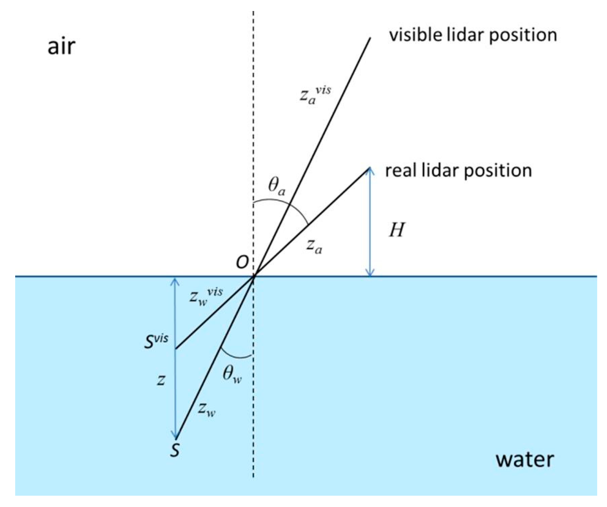
Consider two Cartesian coordinate systems, $(x_a,y_a,z_a)$ and $(x_w,y_w,z_w)$, as shown in Figure 1, where the subscripts a and w stand for atmosphere and water, respectively. The z_a-and z_w-axes coincide with the lidar axis in the atmosphere and in the water, respectively; i.e., the z_w-axes is the z_a-axes refracted with the water surface. Both have the origin O at the intersection with the water surface. The inclinations of these axes are ${\theta }_a$ and ${\theta }_w$ from the zenith, being related by Snell’s law. The x_a-and x_w-axes are both in the principal plane—the plane of the lidar axis and vertical direction—and directed upward. The y_a-and y_w-axes are both perpendicular to the principal plane. Vectors $r_a=(x_a,y_a)$ and $r_w=(x_w,y_w)$ define the position of the point in the plane, perpendicular to O-z_a and O-z_w, and vectors $n_a$ and $n_w$ define the projection of the unit vector of light propagation onto these planes. The altitude of the lidar is $H$, which gives the position $(0,0,-z_a)=(0,0,-H\sec {\theta }_a)$, where $z_a$ is the path length in atmosphere. The underwater point from which the signal is coming has coordinates $(0,0,z_w)=(0,0,z\sec {\theta }_w)$, where $z_w$ is the path length in water and $z$ is the point depth.

The lidar signal $P(z_w)$ is the received radiative energy $\mathrm{\Delta }E$ per path length $\mathrm{\Delta }{z}_w$ independent of the path length $z_w$, which is related to the photon arrival time $t$ as $t=2z_a/V+2n{z}_w/V$, where $V$ is the speed of light in air and $n$ is the refractive index of water. In the framework of the quasi-single (QS) approximation, the lidar signal can be written as [12]

$$P(z_w)=W_{0}b(z_w){\displaystyle \int \mathrm{d}{r}_w{\displaystyle \int \mathrm{d}{n}_w^{\prime }{\displaystyle \int \mathrm{d}{n}_w^{″}{I}_{src}(z_w,r_w,n_w^{\prime }){\tilde{\beta }}^b(z_w;\left|n_w^{\prime }-n_w^{″}\right|)}}}{I}_{src}^{rec}(z_w,r_w,n_w^{″}),$$

(1)

where $W_0$ is the laser pulse energy, $b(z_w)$ is the scattering coefficient along the beam path, ${\tilde{\beta }}^b(z_w,\theta )$ is the backscattering phase function, ${\tilde{\beta }}^b(z_w,\theta )=\tilde{\beta }(z_w,\pi -\theta )$, where $(\pi -\theta )$ is the scattering angle and $\tilde{\beta }(z_w,\theta )$ is the phase function, and $I_{src}(z_w,r_w,n_w)$ and $I_{src}^{rec}(z_w,r_w,n_w)$ describe the angular distributions of radiance at the underwater point $(z_w,r_w)$, due to the real and fictitious sources of unit power with the spatial–angular diagrams ${\phi }_{src}(r_a,n_a)$ and ${\phi }_{rec}(r_a,n_a)$, corresponding to the real laser and receiver, respectively.

The solution of the problem that explicitly relates the signal to the lidar system and turbid medium characteristics is found with the small-angle (SA) approximation [12]:

$$\{\begin{array}{cc}\hfill P(z_w)& =W_{0}b(z_w){\displaystyle \int \frac{\mathrm{d}q\mathrm{d}p}{{(2\pi )}^4}{\tilde{\beta }}^b(z_w,p)I_{eff}(z_w,q,p)}\hfill \\ \hfill I_{eff}(z_w,q,p)& =T^2({\theta }_a){\phi }^{vis}\left(q,p+q(z_w+z_{a}n)\right)\hfill \\ & \times \exp \left(-{\displaystyle {\int }_0^{z_w}2\left\{c(\xi )-b(\xi ){\tilde{\beta }}^f\left(\xi ,\left|p+q(z_w-\xi )\right|\right)\right\}\mathrm{d}\xi }\right)\\ \hfill {\phi }^{vis}(q,p)& ={\phi }_{src}^{*}\left(\eta q_x,q_y;\frac{\eta }{n}{p}_x,\frac{1}{n}{p}_y\right){\phi }_{rec}\left(\eta q_x,q_y;\frac{\eta }{n}{p}_x,\frac{1}{n}{p}_y\right)\hfill \end{array},$$

(2)

where $q$ and $p$ are the vectors in the frequency domain, $T({\theta }_a)$ is the Fresnel transmittance through the boundary at incident angle ${\theta }_a$, $c(z)$ is the beam attenuation coefficient, the superscript vis denotes the source and receiver as visible from under water (see Figure 1 and Appendix A), and ${\phi }_{src}(q,p)$ and ${\phi }_{rec}(q,p)$ are the Fourier transforms of the source and receiver functions (* represents complex conjugation)

$${\phi }_{rec,src}(q,p)={\displaystyle \int \mathrm{d}r\mathrm{d}n{\phi }_{rec,src}(r,n)\exp \left(iq\cdot r+ip\cdot n\right)},$$

(3)

and

$$\eta =\frac{\cos {\theta }_a}{\cos {\theta }_w}.$$

(4)

${\tilde{\beta }}^b(p)$ and ${\tilde{\beta }}^f(p)$ are the Hankel transforms of the backward and forward phase functions:

$${\tilde{\beta }}^{b,f}(p)=2\pi {\displaystyle \underset{0}{\overset{\infty }{\int }}{\tilde{\beta }}^{b,f}(\theta )J_0(p\theta )\theta \mathrm{d}\theta },$$

(5)

where $J_0(x)$ is the Bessel function of the zero order.

As shown in [13], if the backscattering is isotropic (${\tilde{\beta }}^b(\theta )=const$), Equation (2) becomes simpler:

$$P(z_w)=W_0{\beta }^{\pi }(z_w){\displaystyle \int \frac{\mathrm{d}q}{{(2\pi )}^2}{I}_{eff}(z_w,q,p=0)},$$

(6)

where ${\beta }^{\pi }(z_w)$ is the volume scattering function at 180°, which is the product of $b(z_w)$ and ${\tilde{\beta }}^b(0)$.

In summary, the analytical model is based on the quasi-single (QS) and the small-angle (SA) approximations. The QS approximation gives us Equation (1), and the use of the SA approximation provides the explicit solution given by Equations (2) and (6).

The statistical parameters that reflect the accuracy of the analytical model are defined as follows. The coefficient of determination R² is used to describe the goodness of fit; that is,

$$R^2=1-\frac{{\displaystyle \sum _{i=1}^m{(\log f_i-\log y_i)}^2}}{{\displaystyle \sum _{i=1}^m{(\overline{\log y}-\log y_i)}^2}},$$

(7)

where m is the sample number, $f_i$ and $y_i$ are predicted values, e.g., MC or experimental results, and original values, namely the analytical model, respectively, and $\overline{\log y}$ is the average of the logarithm of original values. The reason for employing the logarithm is to avoid ignoring the deviation of weak signals, because the dynamic ranges of lidar signals span several orders of magnitude. The root mean square of relative difference between the original and predicted values $\delta$ is written as

$$\delta =\sqrt{\frac{1}{m}{\displaystyle \sum _{i=1}^m{(1-y_i/f_i)}^2}}.$$

(8)

3. Monte Carlo Validations

The comparisons between the analytical model described in Section 2 and the MC simulation are presented in this section. The standard MC (stan-MC) and semi-analytic MC (semi-MC) algorithms are employed to provide MC-simulated results. The stan-MC algorithm refers to the method described in [9], where a large number of photons are used in a purely stochastic construction of the trajectories to measure the relevant information. According to the radiative transfer equation, the lengths and directions of the trajectories are determined by the optical properties of the water. However, due to the low backscattering probability and limited lidar receiving area, only a small number of photons can meet the receiving conditions even if a large number of photons are emitted. If the number of photons is insufficient, a large statistical error is unavoidable for the stan-MC method. Compared with the stan-MC algorithm, the semi-MC algorithm greatly reduces the variance by combining stochastic processes and analytical estimates. The semi-MC algorithm refers to the method illustrated in [8], where an analytical estimate is calculated for the possibility of the collection of scattered photons at certain points, and the estimate is added into the signals. The estimate can be written as

$$E=\tilde{\beta }(\theta )\mathrm{\Delta }\mathrm{\Omega }\exp (-c{L}_0)T_s,$$

(9)

where $\tilde{\beta }\left(\theta \right)$ is the phase function at the mean scattering angle θ where the photons scatter into the receiving solid angle. The term exp(-cL₀) is the probability that the photons scattered through angle θ will be transmitted from the present point to the air–water interface with a distance of L₀, where c is the beam attenuation coefficient.

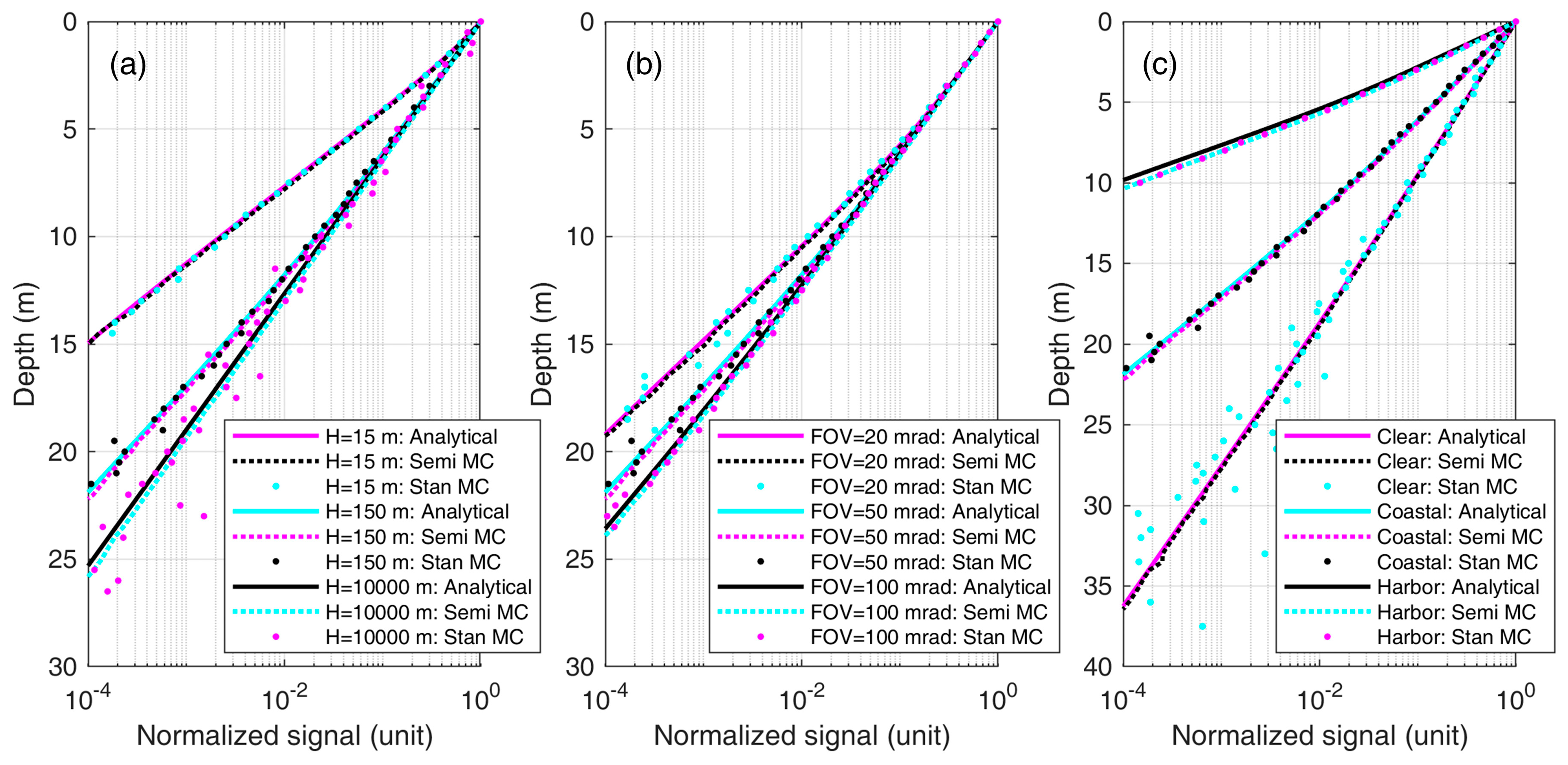
3.1. Homogeneous Water

The simulation parameters in homogeneous water are listed in

Table 1. Simulation parameters in homogeneous water. FOV: field of view.

Cases	1	2	3	4	5	6	7
Telescope diameter (cm)	10	20	100	20	20	20	20
Working altitude (m)	15	150	10,000	150	150	150	150
Receiver FOV (mrad)	50	50	50	100	20	50	50
Water type	Coastal	Coastal	Coastal	Coastal	Coastal	Clear	Turbid
Absorption (m−1)	0.179	0.179	0.179	0.179	0.179	0.114	0.366
Scattering (m−1)	0.219	0.219	0.219	0.219	0.219	0.037	1.824
Backscatter fraction	0.013	0.013	0.013	0.013	0.013	0.044	0.020
Average cosine	0.9247	0.9247	0.9247	0.9247	0.9247	0.9247	0.9247

. The parameters—e.g., the working altitude, receiver field of view (FOV) and water type—are variable to investigate their effects on the accuracy of the analytical model [16]. The working altitudes from the lidar to the water surface are set at 15, 150 and 10,000 m (Cases 1–3 in Table 1), corresponding to the working altitude of the shipborne [17,18], low-altitude airborne [19] and high-altitude airborne oceanic lidars [20], respectively. The FOVs are selected at 20, 50, and 100 mrad (Cases 5, 2, and 4 in Table 1). The water types cover the clear ocean, coastal ocean and turbid harbor (Cases 6, 2 and 7 in Table 1) and refer to Petzold’s data [10,21]. The backscatter fraction is the ratio of the backscattering coefficient to the scattering coefficient. The backward phase function is assumed to be uniform, while the forward phase function is determined by the Dolin model [22] and can be calculated from the average cosine of the scattering angle [23]. The effects of the telescope diameter, laser diameter and divergence angle on the lidar signals are small and are therefore not discussed here because of the large product of the FOV and working altitude [16]. The laser diameter and divergence angle are set to be infinitesimal. The oceanic lidar points to the nadir. The laser wavelength is 532 nm, and the telescope diameters are larger at higher working altitudes to reduce the variance of the stan-MC simulation. Each profile of the semi-MC and stan-MC simulation is simulated with inputs of 5 × 10⁹ and 5 × 10¹² photons, respectively.

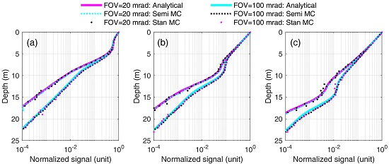
The lidar signals calculated by the analytical model, semi-MC and stan-MC algorithms are shown in Figure 2. The effects of altitude (Cases 1–3 in Table 1), FOV (Cases 4, 2 and 5 in Table 1) and water type (Cases 6, 2 and 7 in Table 1) are shown in Figure 2a–c, respectively. To give a more explicit picture, the lidar signals are normalized by their maximums, and the dynamic ranges are set to 4 orders of magnitude. In Figure 2, the results of the three algorithms agree very well at different conditions. The quantitative analysis of the accuracy of the analytical model—e.g., the coefficient of determination R² and the root mean square of the relative difference δ described in Section 2—is shown in

Table 2. The R² and δ of the analytical model compared with the semi-analytic and standard MC algorithms according to Figure 2.

Cases		1	2	3	4	5	6	7	Total
Semi-MC	R2	0.9995	0.9992	0.9982	0.9994	0.9989	0.9997	0.9875	0.9985
	δ	0.0573	0.0686	0.1050	0.0612	0.0818	0.0425	0.2415	0.0924
Standard MC	R2	0.9987	0.9976	0.9689	0.9918	0.9983	0.9446	0.9893	0.9789
	δ	0.0837	0.1349	0.5011	0.2016	0.1053	1.1460	0.2236	0.6104

. Compared with the semi-MC results, δ values are within 7% in Cases 1, 2, 4, and 6, but are slightly larger in Case 3, 5 and 7, which may be caused by the intensity of multiple scattering at large angles. The accuracy of the analytical model is expected to increase with the greater contribution of small-angle scattering—i.e., for smaller FOVs and their footprints—for clearer waters with stronger phase function peaks. The maximum difference is in Case 7, which is outstanding because of the extremely turbid water. In this case, the scattering at large angles predominates and the small-angle approximation used in the analytical model loses its accuracy. However, it is worthy of note that, with scattering at large angles, the relationship $t=2z_a/V+2n{z}_w/V$ between the photon arrival time and the depth from which the signal comes is violated, so these cases are not informative from the point of view of lidar sounding. The total R² and δ considering Cases 1–7 in Table 1 are 0.9985 and 9.24% for semi-MC. Values of δ for semi-MC are significantly higher than δ for stan-MC, which demonstrates the advantage of semi-MC in terms of the variance reduction. Nevertheless, R² values are very high, which can also verify the accuracy of the analytical model. In conclusion, the analytical model agrees with MC simulations very well in homogeneous water.

The measurement geometry and medium optical properties determine the lidar signals. As shown in Figure 2a, a high altitude leads to a low attenuation of the signal. For the same FOV, the higher altitude lidar can “see” a larger volume and can collect more multiple scattering signals. In order to “see” the same volume, the lower lidar should have a larger FOV. As shown in Figure 2b, a small FOV corresponds to a large attenuation of the signal because a small FOV limits the reception of photons. Furthermore, all signals are almost the same within a depth of 3 m, but the signal of 20 mrad is weaker than the others beyond a depth of 3 m because of larger multiple scattering in the deeper water. Therefore, a large FOV is beneficial to detect deep signals, and a small FOV is enough to detect shallow signals. Seawater optical properties are the main external factors affecting lidar signals, as shown in Figure 2c. Lidar signals attenuate faster in more turbid water. For example, within the dynamic range of four orders of magnitude, the signal can reach a depth of 35 m in the clear ocean, which is 1.6 times and 3.2 times that in the coastal ocean and turbid harbor, respectively. The detection depth is more related to the absorption coefficient than the scattering coefficient because the photons scattered in the water are not completely lost, and a large proportion of the photons undergoing forward multiple scattering still contribute to the lidar signal.

3.2. Inhomogeneous Water

The analytical model can be used to investigate lidar signals in inhomogeneous water, which exists widely in the ocean. Consider inhomogeneous water comprising a uniform background and a phytoplankton layer; the background optical properties of the water body refer to the coastal ocean in Table 1. The depth-resolved chlorophyll concentration of the phytoplankton layer, which is Gaussian-like, can be written as [24]

$$C(z)=C_L\exp \left[-\frac{{(z-z_L)}^2}{w_L^2}\right],$$

(10)

where $C_L$ is the peak concentration of the layer, $z$ is the depth, $z_L$ is the peak depth of the layer, and $w_L$ is the thickness of the layer. Then, the absorption coefficient and scattering coefficient can be calculated from the bio-optical model [25]. In the simulation, $C_L$ is 1 mg·m⁻³, $w_L$ is 2 m, the oceanic lidar is pointing to the nadir, the laser wavelength is 532 nm, the telescope diameter is 20 cm, and the working altitude is 150 m. z_L and FOV are listed in

Table 3. Simulation parameters in inhomogeneous water.

Cases	1	2	3	4	5	6
zL (m)	5	5	10	10	15	15
FOV (mrad)	20	100	20	100	20	100

for Cases 1–6 to investigate their effects on the accuracy of the analytical model.

The lidar signals in inhomogeneous water calculated by the analytical model, semi-MC algorithm and stan-MC algorithm are shown in Figure 3. The results of $z_L$ at 5 m (Cases 1–2 in Table 3), 10 m (Cases 3–4 in Table 3) and 15 m (Cases 5–6 in Table 3) are shown in Figure 3a–c, respectively. The results of the three models agree well, but there are subtle differences at the boundaries of the layers. Quantitatively,

Table 4. The R² and δ of the analytical model compared with the semi-analytic and standard MC algorithms according to Figure 3.

Cases		1	2	3	4	5	6	Total
Semi-MC	R2	0.9991	0.9982	0.9985	0.9977	0.9988	0.9965	0.9981
	δ	0.0870	0.1117	0.0944	0.1196	0.0807	0.1319	0.1077
Stan-MC	R2	0.9981	0.9976	0.9964	0.9979	0.9943	0.9963	0.9970
	δ	0.1337	0.1223	0.1372	0.1166	0.1784	0.1412	0.1386

demonstrates the R² and δ of the analytical model in inhomogeneous water. It shows that the total R² and δ considering Cases 1–6 in Table 3 are 0.9981 and 10.77% for semi-MC. R² values are very high for stan-MC, which can also verify the accuracy of the analytical model. Therefore, the analytical model described in Section 2 is verified to give high accuracy in inhomogeneous water.

In Figure 3, the subtle differences between the analytical model and MC simulation are caused by the multiple-scattering-induced temporal spread of the laser pulse. The spread cannot be recorded by the analytical model described in Section 2 [13], but can be both presented by the semi-analytic and standard MC algorithms. The spreads manifest as rising and falling delays in the layer boundaries. The delays with an FOV of 100 mrad are slightly greater than those with 20 mrad because the returning photons that cause the temporal spread mainly have large angles of incidence. In Table 4, the δ of 10.77% for semi-MC seems acceptable for most oceanic lidars, because seawater phase functions are strongly peaked and the spread is proportional to the 4th moment $\langle {\theta }^4\rangle$ of the forward phase function. Therefore, the analytical model in its classical form described in Section 2 is usually used and is expected to give high accuracy. If the temporal spread cannot be ignored, the modified analytical model developed in [26] that includes the temporal spread could be used [27].

4. Experimental Validations

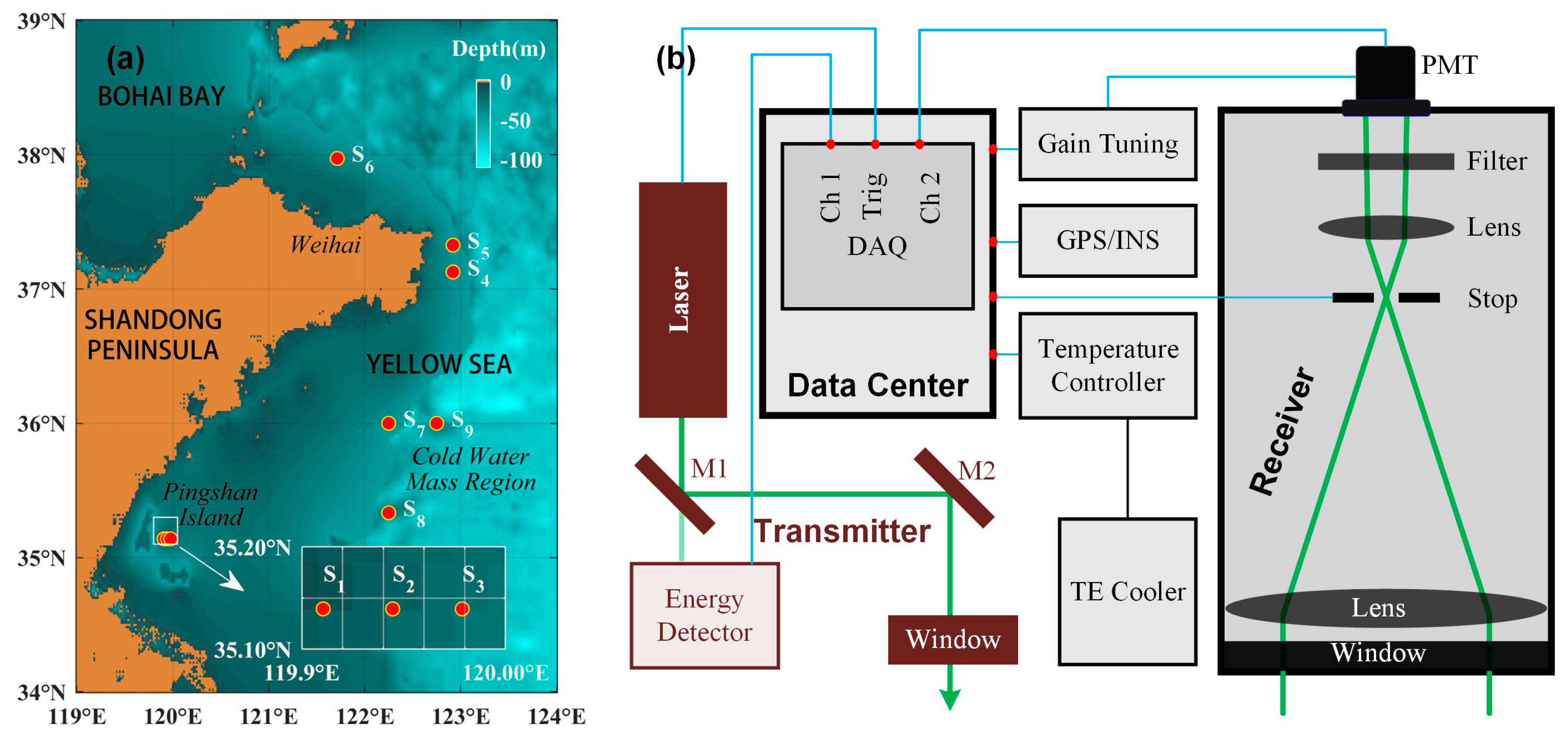
This section compares lidar signals calculated by the analytical model described in Section 2 with the field experimental results. In August 2017, a field experiment was carried out with the R/V Haili in the Yellow Sea near the Shandong Peninsula. As shown in Figure 4a, 9 stations were used for the experimental validation. The digital topographic data are from the ETOPO1 Global Relief Model published by the National Geophysical Data Center (NGDC) [28]. ETOPO1 is a 1 arc-minute global relief model of Earth’s surface that integrates land topography and ocean bathymetry. Stations 1–3 are around Pingshan Island at shallow depths. Stations 4–6 are near the coastline of Weihai and are slightly deeper than Stations 1–3. Stations 7–9 are in the cold water mass region of the Yellow Sea with larger depths than Stations 4–6. The data from different stations are helpful in illustrating the reliability of the analytical model. Synchronous observations of the lidar and in situ instruments were carried out on the ship.

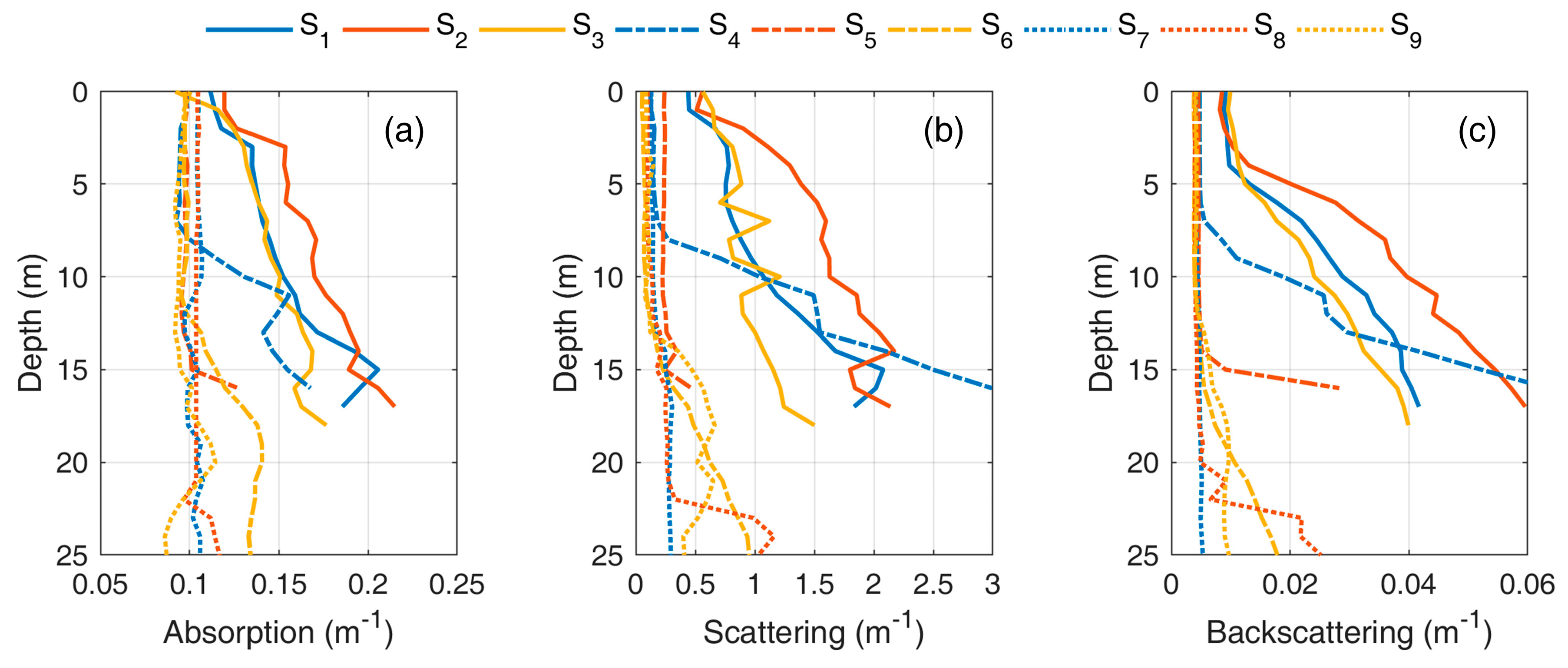
The shipborne oceanic lidar developed by Zhejiang University was fixed in the front of the ship with an altitude of approximately 9 m and an angle of incidence of approximately 50° from the nadir. The biaxial lidar transmitted a laser pulse into the seawater and detected the lidar returns for the retrieval of the seawater optical properties, as shown in Figure 4b. This mainly consisted of a transmitter, a receiver and a data center. The transmitter included a frequency-doubling Q-switched Nd:YAG pulsed laser at 532 nm, with a single pulse energy of 5 mJ, a pulse width of 10 ns and a repetition frequency of 10 Hz. The diameter of the laser was 8 mm with an angle of divergence of 1 mrad. The laser beam was launched into the seawater through a series of reflectors and an optical window. The receiver consisted of a telescope, a stop, an interference filter, a collimating lens and a photomultiplier tube (PMT). The diameter of the telescope was 80 mm, and the FOV was tunable to collect backscattering light from seawater. The overlap region reached a unit after approximately 0.5–2 m for the FOVs in the experiment. The data center collected lidar signals and additional information about the lidar working states. It consisted of a high-speed data acquisition (DAQ) card with a sampling frequency of 500 MHz and a series of accessories. The gain of the PMT was recorded during measurement for the calibration. The background signal was calculated by the signal average at a depth of 100–200 m and then removed from the lidar signals. The effective depth resolution was approximately 0.92 m due to the limitation of the laser pulse width. Then, for convenient comparison, the depth resolutions of lidar-measured signals were changed to 1 m through the linear interpolation. The accessories included a temperature controller and GPS/INS, etc., which can obtain additional information and feedback from the other components. Each lidar-measured signal was an average of 100 groups (10 s) of lidar-measured original signals to reduce the effect of random noises and a wavy surface.

In situ equipment was lowered into the seawater by a winch on the back deck of the ship to collect inherent optical properties. The absorption coefficient and beam attenuation coefficient were collected using WET–Labs ac-9 at 532 nm. The scattering error in the particulate absorption measurement was corrected following the procedure in [29]. The backscattering coefficient at 488 nm and 550 nm was estimated from measured scattering at a given angle (~140 degrees) by HOBILabs HS6P. The standard percentage error in this estimate was believed to be ~9% [30]. Sigma correction was made to the original backscattering following the HOBILabs operation manual [31]. The backscattering coefficient at 532 nm was linearly interpolated between the values at 488 nm and 550 nm. All in situ data were then binned to a depth resolution of 1 m through the quality control, as shown in Figure 5. Stations 1–3 were very turbid, which might be attributed to the strong resuspension of sediment and terrestrial inputs of particulate matter. Also, Station 4 was turbid beyond the depth of 7 m, which might be related to the internal wave.

The analytical model is configured with the lidar system parameters—e.g., the FOV and receiver diameter—and seawater optical properties—e.g., the absorption, scattering, backscattering and phase function—to produce the lidar signals. The diameter of the laser was 8 mm with a divergence of 1 mrad. As these parameters are much smaller than those of the receiver, we assume that the spatial–angular distribution of the laser is uniform. We neglect the distance between the laser and receiver, because the distance is very small, at about 5 cm, and the receiver FOV is large, so the full overlap is reached at 0.5–2 m for various FOVs in the experiment. Most of the seawater optical properties can be obtained by in situ measurements, except the phase function, due to the limited equipment. Many different phase functions have been used in marine optics including measured, analytical and theoretical ones. Among them, the Fournier–Forand (FF) phase function based on Mie theory is proven to give good predictions with measured phase functions [32]. Here, FF phase functions are calculated with particulate backscatter fractions following the method proposed by Mobley [32]. The backscattering phase function is assumed to be isotropic. Furthermore, we convolve signals calculated by the analytical model with the system time response related to the detector and laser that is calibrated in advance. The air–sea interface is assumed to have a zero longitudinal slope in the simulation because the water surface is relatively smooth in the experiment. The reflection of the water surface is not considered in the analytical model because the incidence angle is relatively large.

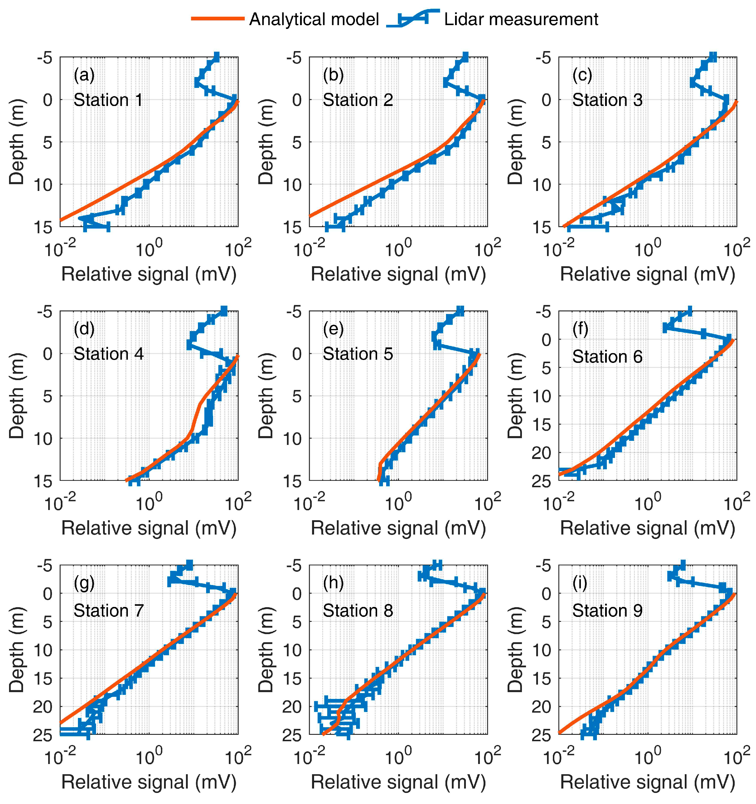
4.1. Different Turbidity

Figure 6 shows the lidar signals calculated by the analytical model (orange solid lines) and measured by the lidar (blue solid lines with error bars) with a large, full FOV of 200 mrad. Stations 1–9 correspond to Figure 6a–i, respectively. The average values in blue solid lines and standard deviations in blue error bars are plotted from 10 lidar-measured signals during the in situ operation period. The negative depth indicates the information above the water surface. Generally, the backscattering in the atmosphere is much weaker than that in the seawater. To ensure the dynamic range of the lidar, the detector gains at different stations are adjusted to control the maximum signal close to 100 mV. Dynamic ranges of 3–4 orders of magnitude can then be realized in most cases. As shown in Figure 6, the analytical model can match the lidar-measured results in different turbidities.

Table 5. The R² and δ of the analytical model compared with the lidar measurement in different turbidities.

Stations	1	2	3	4	5	6	7	8	9	Total
R2	0.8723	0.8737	0.9410	0.8843	0.9811	0.9653	0.9507	0.9874	0.9595	0.9429
δ	0.5234	0.5642	0.4713	0.8479	0.2146	0.4248	0.4019	0.2409	0.3256	0.4570

lists the R² and δ of the analytical model compared with the lidar measurement. For statistical calculations, the depth ranges of 0~15 m are considered for S₁-S_5, and the depth ranges of 0~25 m are considered for S₆-S₉. S₁–S₄ present large δ values, which may be caused by the sediment fluctuation or assumed phase functions during the measurement. The total R² and δ considering all cases are 0.9429 and 45.7%, which means that the analytical model performs well with a large FOV in different turbidities. The results verify the potential of the analytical model in the simulation of lidars with large footprints, which might also be suitable for some recently developed oceanic lidars [17,20,33].

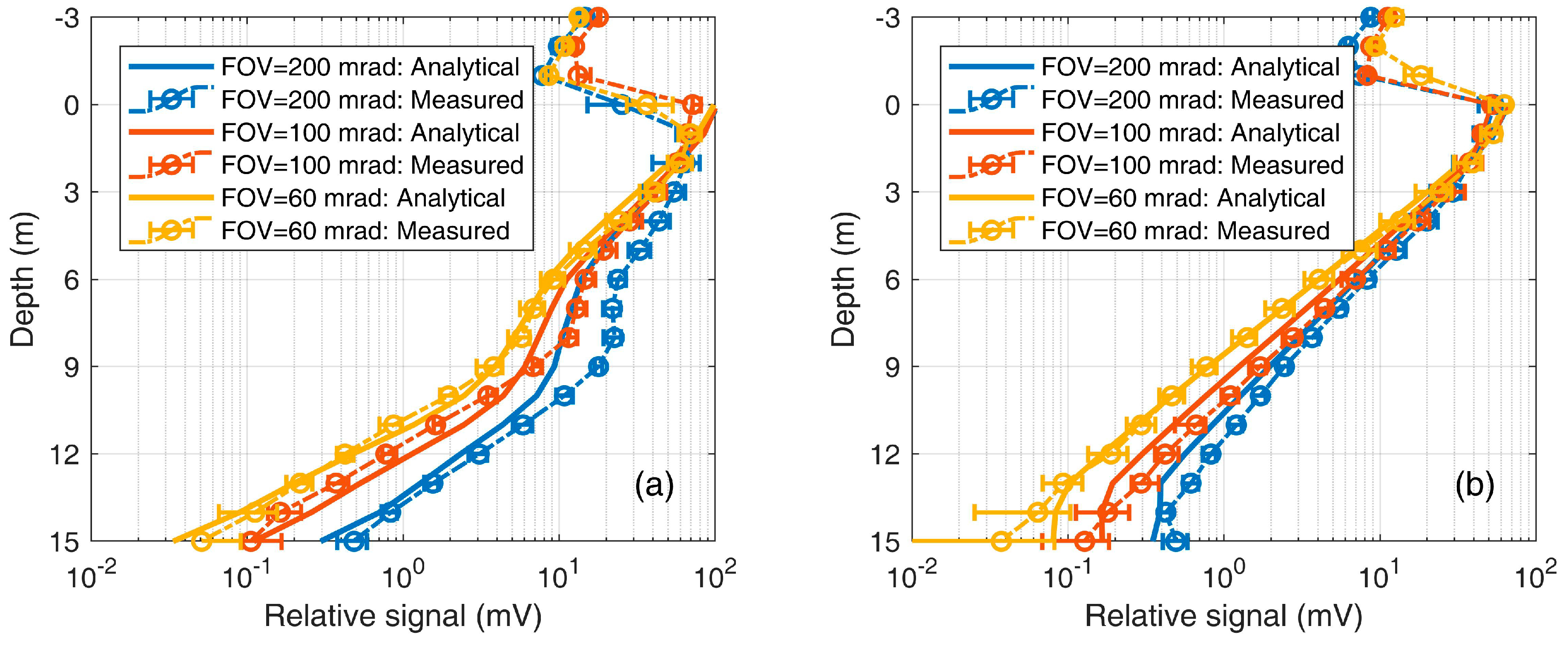
4.2. Different Fields of View

As illustrated in Section 2, two system parameters—i.e., the working altitude and the receiver FOV—are the keys to studying multiple scattering. In the shipborne case, it is difficult to change the altitude but easy to change the FOV with a variable field stop. Therefore, the analytical model (solid lines) is compared with lidar-measured signals (dashed–dotted lines with circles and error bars) at Stations 4–5 with multiple full FOVs, viz. 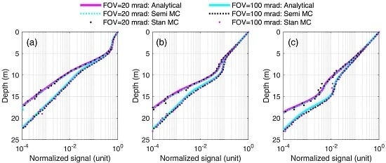60, 100 and 200 mrad, as shown in Figure 7. The experimental results are calculated from 10 lidar-measured signals during the in situ operation period. Good agreement can be observed between the simulation and measurement. Also, it is shown that a small FOV corresponds to a large attenuation of the lidar signal. Therefore, a large FOV is beneficial to the detection of deep information.

Table 6. The R² and δ of the analytical model to lidar measurement with different FOVs at Stations 4–5.

Stations	4			5			Total
FOV (mrad)	200	100	60	200	100	60
R2	0.8843	0.9779	0.982	0.9811	0.9837	0.9908	0.9744
δ	0.8479	0.3251	0.4618	0.2146	0.2363	0.3074	0.4536

lists the R² and δ of the analytical model compared with lidar measurement with different FOVs at Stations 4–5. S₄ presents a larger δ than S₅, because of the possible instability of the water body. Furthermore, the total R² and δ considering all cases are 0.9744 and 45.36%. Therefore, the practicality of the analytical model in the simulation of the multiple-field-of-view lidar is verified.

5. Discussion

The validation of the analytical model is an important contribution to the field of oceanic lidar sounding, not only because the analytical model can calculate lidar signals accurately and efficiently, but also because it provides a clear physical insight to the process of lidar signal forming and allows one to look at the inversion of lidar waveforms from the analytical or semi-analytical point of view, which is impossible when using Monte Carlo methods. The analytical model presents good agreement with the semi-MC simulation in homogeneous and inhomogeneous waters. The total R² and δ comprising all the semi-MC simulation are 0.9983 and 9.82%, respectively. The analytical model in its classical form described in Section 2 is expected to give high accuracy, although slight errors may be introduced due to QSSA’s approximation of the analytical model and the noise of MC fluctuation. The analytical model and lidar experiment show strong correlation for various turbidities with a large field of view and for moderate turbidity with various fields of view. The total R² and δ comprising all the experimental data are 0.9516 and 45.58%, respectively. The accuracies suffer from possible errors of the lidar experiment—e.g., the detector gain fluctuation and signal noises in deep water—and possible errors of the in situ data caused by the distance between the in situ and lidar measurements, anchor dropping in Stations 1 and 2 and additional turbulence caused by the ship’s propeller, which both could provide horizontal water inhomogeneity by lifting silt from the bottom. Notably, the phase function is not measured directly due to the limited equipment, but is generated from the in situ depth-resolved backscatter fraction [32]. The assumed phase function might be an important error source. The water surface effects on the lidar signals are not considered in the analytical model. The effects of the surface reflection on lidar signals and the effects of water surface roughness on changing the normal vector of the incident surface are both possible error sources. These errors could be reduced by an upgraded gain controller, in situ phase function measurement, better experimental designs and a consideration of the surface roughness in future.

The most important application of the analytical model is in investigating the retrieval of the sea water properties from an oceanic lidar waveform. During the retrieval, the lidar equation for nadir incidence is often written in the single scattering approximation [4]:

$$P(z)=\frac{C{{\beta }^{\prime }}^{\pi }(z)}{{(nH+z)}^2}\exp \left[-2{\displaystyle {\int }_0^z\alpha (\xi )d\xi }\right],$$

(11)

where $C$ is the system constant and ${{\beta }^{\prime }}^{\pi }(z)$ is the effective volume scattering function at 180°, which represents the ability of the seawater to scatter light back into the direction of the receiver, $\alpha (z)$ is the lidar attenuation coefficient, and $\exp \left[-2{\displaystyle {\int }_0^z\alpha (\xi )d\xi }\right]$ describes how much light is lost from the lidar to depth $z$ and back [5]. When backscattering is not isotropic, ${{\beta }^{\prime }}^{\pi }(z)$ is not equal to the volume scattering function at 180° ${\beta }^{\pi }(z)$, because of multiple scattering, as the backscattering angles deviate from 180°. Conversely, if backscattering is isotropic, ${{\beta }^{\prime }}^{\pi }(z)$ is hardly affected by multiple scattering [34,35]. $\alpha (z)$ is closely related to the measurement geometry and the seawater optical properties. If ${\beta }^{\pi }(z)$ does not change with depth—e.g., for isotropic backscattering and homogeneous water—$\alpha (z)$ can be written as

$$\alpha (z)=-\mathrm{d}\ln \left[\frac{P(z){(nH+z)}^2}{C{\beta }^{\pi }}\right]/2\mathrm{d}z,$$

(12)

Gordon concluded that $\alpha$ corresponds to the beam attenuation in a small FOV and to the diffuse attenuation K_d in a large FOV, according to simulated lidar signals at a shallow depth [16]. In field experiments, the $\alpha$ measured by Lee et al. [33] is approximated to K_d, the $\alpha$ measured by Schulien et al. [20] is approximated to but slightly larger than K_d, and the $\alpha$ measured by Collister et al. [17] is close to a. The simple conclusion that $\alpha$ is approximate to one of the optical properties is useful but not sufficient for the retrieval of the lidar returns. Theoretically, Walker and McLean [10] concluded that $\alpha$ is variable with depth: it is close to a at the water surface and to K_d in deep water. Liu et al. [36] investigates the relationships between $\alpha$ and the inherent optical properties of seawater for spaceborne lidars. The analytical model in this paper also presents results similar to the results of Walker and McLean [10], as shown in Figure 8. However, in practical conditions, surface reflection and lidar system response may increase the uncertainty at the water surface, and system noises may introduce large errors in deep water. 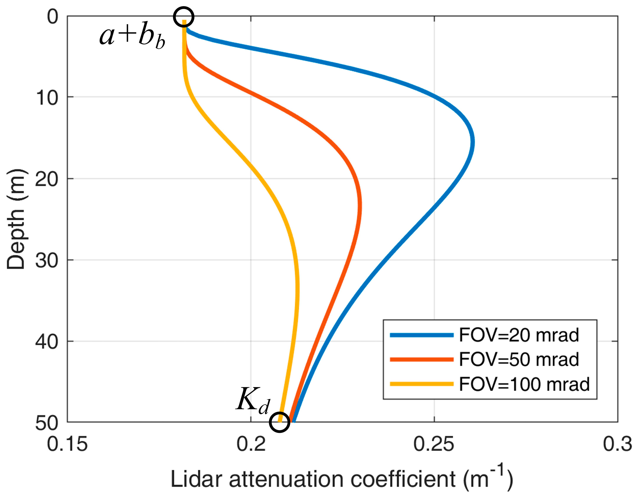Therefore, further studies that efficiently and accurately correct $\alpha$ at full depths to an inherent optical property are expected based on the analytical model. Additionally, the ability to simulate signals in inhomogeneous water makes the analytical model attractive and practical in the actual ocean.

As indicated in Figure 8, there is another research direction in which more information about optical properties can be obtained from the lidar attenuation coefficient with different FOVs. In terms of atmospheric lidar, Bissonnette et al. [37] and Schmidt et al., [38] carried out studies on the atmospheric multiple-FOV lidar and proposed a series of theoretical methods for retrieving the cloud extinction coefficient and droplet effective diameter. It is possible to use the analytical model to retrieve multiple optical and microphysical properties accurately and efficiently from oceanic multiple field-of-view lidar signals [39,40]; e.g., scattering, absorption, diffuse attenuation, phase function and hydrosol characteristics. In future, the theories and hardware of oceanic multiple-FOV lidar are expected to investigate the information within multiple scattering.

6. Conclusions

The analytical model, which is based on the quasi-single small-angle scattering approximation, can efficiently simulate oceanic lidar signals with multiple scattering. The model is modified to include refraction at oblique incidence and is then compared with Monte Carlo (MC) simulations and experimental results. Under different working conditions, the results calculated by the analytical model demonstrated very good agreement with the MC simulation and experimental data. The analytical model presents good agreement with the semi-analytic MC simulation in homogeneous (R² = 0.9985, δ = 9.24%) and inhomogeneous waters (R² = 0.9981, δ = 10.77%). The analytical model and lidar experiment show a strong correlation for various turbidities with a large field of view (R² = 0. 9595, δ = 45.7%) and moderate turbidity with various fields of view (R² = 0.9744, δ = 45.36%). The results validate the analytical model in the simulation of the oceanic lidar signals. The analytical model is expected to accurately and efficiently retrieve various seawater optical properties from the lidar waveforms measured under strong multiple scattering conditions.