Article

Mapping Irrigated Areas Using Sentinel-1 Time Series in Catalonia, Spain

1
IRSTEA, TETIS, University of Montpellier, 500 rue François Breton, 34093 Montpellier CEDEX 5, France
2
CESBIO (CNRS/UPS/IRD/CNES/INRA), 18 av. Edouard Belin, bpi 2801, 31401 Toulouse CEDEX 9, France
3
CIHEAM-IAMM, UMR-System, 34090 Montpellier, France
4
isardSAT, Parc Tecnològic Barcelona Activa, Carrer de Marie Curie, 8, 08042 Barcelona, Catalunya, Spain
*
Author to whom correspondence should be addressed.
Remote Sens. 2019, 11(15), 1836; https://doi.org/10.3390/rs11151836
Submission received: 1 July 2019 / Revised: 2 August 2019 / Accepted: 4 August 2019 / Published: 6 August 2019

Abstract

:
Mapping irrigated plots is essential for better water resource management. Today, the free and open access Sentinel-1 (S1) and Sentinel-2 (S2) data with high revisit time offers a powerful tool for irrigation mapping at plot scale. Up to date, few studies have used S1 and S2 data to provide approaches for mapping irrigated plots. This study proposes a method to map irrigated plots using S1 SAR (synthetic aperture radar) time series. First, a dense temporal series of S1 backscattering coefficients were obtained at plot scale in VV (Vertical-Vertical) and VH (Vertical-Horizontal) polarizations over a study site located in Catalonia, Spain. In order to remove the ambiguity between rainfall and irrigation events, the S1 signal obtained at plot scale was used conjointly to S1 signal obtained at a grid scale (10 km × 10 km). Later, two mathematical transformations, including the principal component analysis (PCA) and the wavelet transformation (WT), were applied to the several SAR temporal series obtained in both VV and VH polarization. Irrigated areas were then classified using the principal component (PC) dimensions and the WT coefficients in two different random forest (RF) classifiers. Another classification approach using one dimensional convolutional neural network (CNN) was also performed on the obtained S1 temporal series. The results derived from the RF classifiers with S1 data show high overall accuracy using the PC values (90.7%) and the WT coefficients (89.1%). By applying the CNN approach on SAR data, a significant overall accuracy of 94.1% was obtained. The potential of optical images to map irrigated areas by the mean of a normalized differential vegetation index (NDVI) temporal series was also tested in this study in both the RF and the CNN approaches. The overall accuracy obtained using the NDVI in RF classifier reached 89.5% while that in the CNN reached 91.6%. The combined use of optical and radar data slightly enhanced the classification in the RF classifier but did not significantly change the accuracy obtained in the CNN approach using S1 data.

Graphical Abstract

1. Introduction

Under changing climatic conditions, irrigation plays a significant role in agricultural production in order to meet the global food requirement. In fact, better planning of irrigation is required to fulfil the high demand of food with the increase in the global population [1,2]. Moreover, irrigated agriculture accounts now for more than 80% of water withdrawn from rivers, lakes, and groundwater aquifers being the principal consumer of fresh water resources [3,4,5]. Therefore, more focus is being set on the assessment of irrigation performance for improving water management in order to achieve higher water productivity and increase the agricultural water sustainability.
Accurate information on the irrigated area extent helps in managing water resources that affect global food security and in analyzing the impact of climate change on the irrigation water requirement. However, the extent and distribution of irrigated areas remain indefinite in spite of the significant impact of irrigation on food security and water resources. At a global scale, several irrigation products are available at different spatial resolutions. Existing irrigation extent maps such as the FAO (Food and Agriculture Organization of the United Nations) database [6], the Global Map of Irrigated Areas version 5 (GMIA 5.0) [7,8] and the MIRCA2000 product [9] have been primary derived from national statistical data. The Global Rain-Fed Irrigated and Paddy Croplands (GRIPC) with spatial resolution of 500 m was produced using MODIS (Moderate resolution imaging spectroradiometer) satellite data [10]. The low spatial resolution of these products is an obstacle for using them in irrigation management especially in regards to small to medium agricultural areas.
At a regional scale, several efforts have been made to map irrigated areas using remote sensing data including both optical and radar data [11,12,13,14,15,16]. Most studies that use optical data demonstrate that irrigated/non-irrigated areas can be classified based on the difference in temporal signals of vegetation indices such as NDVI (Normalized Differential Vegetation Index), NDWI (Normalized Differential Water Index) and GI (Greenness index) between irrigated and non-irrigated areas. Among optical sensors, MODIS and Landsat have been extensively used to map irrigated areas [12,13,14,15]. For example, Pervez et al. [17] merged the NDVI derived from MODIS at 250 m spatial resolution and used statistical data to map irrigated areas of United States of America in 2002. In their study, they assumed that irrigated crops have a higher annual NDVI peak than non-irrigated crops especially under non-optimal precipitation conditions such as drought. Chen et al. [18] proposed a new approach to map irrigation extent, time and frequency in an arid region located in Hexi Corridor of northwest China by merging the 30 m spatial resolution Landsat images with 250 m MODIS data and ancillary data. In their study, they used the GI to detect irrigation events during the first half of the growing season. The overall accuracy for detecting irrigation water supplements reached 87%. Recently, Xiang et al. [19] mapped irrigated areas of northeast China by comparing the MODIS derived LSWI (Land Surface Water Index) of the agricultural areas to the surrounding natural vegetation such as forests. They assumed that the canopy moisture indicated by the LSWI is higher for irrigated crops than the adjacent forest. Thus, they mapped irrigated areas by fixing a threshold for the difference between LSWI of agricultural plots and that of the forest. However, the overall accuracy of the produced map did not exceed 77.2% with a 0.49 kappa coefficient.
Apart from optical data, recent studies have started exploiting the potential of SAR (synthetic aperture radar) data to map different agricultural irrigated areas [20,21,22,23,24]. The assumption established for using SAR data relies on the fact that radar remote sensing is sensitive to the water content of soil due to the increase in the dielectric constant with the increase of the soil water content. In fact, several studies have reported that the SAR signal is highly affected by soil moisture content [25,26,27,28,29,30]. For example, El-hajj et al. [30] analyzed the sensitivity of radar signals in the X-band over irrigated grassland conditions using time series of TerraSAR-X and Cosmo-SkyMed X-band SAR data. Their results showed that the radar signal in X-band increased by approximately 1.4 dB due to irrigation events occurring one day before the radar acquisition. They concluded that the radar signal could be used to identify three-day-old irrigated plots.
The recently launched Sentinel-1 (S1) SAR satellite offers a powerful tool for agricultural area classification and monitoring under various weather conditions. The S1 satellites (S1A and S1B) provide an exceptional combination of high spatial and high temporal resolutions for dual polarization SAR data (six days of temporal resolution and a 10 m × 10 m pixel spacing) available in free open access mode. S1 time series has been newly exploited by several studies for land cover classification [20,31,32,33]. High quality classification mapping has been produced by applying either classical machine learning, such as random forest and the support vector machine, or complex deep learning methods on S1 time series. Recently, deep learning (DP) techniques [32,34,35] have shown that neural network models are well adapted tools to automatically produce land cover mapping from information coming from both optical [36] and radar [37] sensors. The main characteristic of these models is the ability to simultaneously extract features optimized for image classification. However, only few studies have started exploiting the potential of S1 time series for land cover classification using the DP method. In Interdonato et al. [37] the authors proposed to leverage DP to perform winter quality mapping over a zone in West France. In Ndikumana et al. [31] another DP approach was proposed to perform land cover mapping considering several agricultural classes. Concerning the joint exploitation of radar/optical satellite images based on deep learning techniques, some approaches were recently proposed considering really precise tasks such as image simulation [38] or change detection [39]. Unfortunately, the same opportunity has not been yet fully exploited in the context of land cover mapping.
This study proposes an innovative approach to map irrigated areas at plot scale using the Sentinel-1 and Sentinel-2 (S2) time series. The potential of S1 and S2 acquired at high spatial resolution and high revisit time for irrigation mapping did not yet receive enough attention by the scientific committee. The approach is based on the use of S1 and/or S2 time series combined with statistical and mathematical functions such as the principal component analysis (PCA) and the wavelet transformation (WT) to map irrigated areas. The novelty of this study resides in eliminating the ambiguity between irrigation and rainfall through the comparison between the SAR backscattering signal of each plot and that of the grid (10 km × 10 km) including this plot. To map irrigated areas, the PCA and WT transformation were applied to the S1 time series prepared over a study site located in west of Catalonia, Spain. The PCA was also applied to the NDVI time series derived from the S2 images. Then, random forest (RF) and the convolutional neural network (CNN) approaches were used to build up classification models in three different scenarios: The first using only S1 data, the second using only S2 data, and the third using both S1 and S2 data. Finally, the two classification approaches (RF and CNN) were inter-compared.

2. Materials

2.1. Study Site

The study site examined is the western part of Catalonia region of north east Spain (Figure 1a). Figure 1b shows the location of the S1 footprints used in this study. The area covered by the used footprints corresponds to 55% of the total area of Catalonia and compromises 64% of the total agricultural areas in the region. Figure 1c is a digital elevation model (DEM) derived from the shuttle radar topography mission (SRTM) data and Figure 1d shows the agricultural areas derived from the SIGPAC (geographical information system for agricultural parcels) data of Catalonia. The hatched zone in Figure 1d represents the area finally used in the classification.
Catalonia is a region of 32,000 km2 located in the north east corner of the Iberian Peninsula along the northeastern Spanish Mediterranean coast. The agricultural areas of Catalonia are concentrated in the northeastern part and the interior plane in the western part as shown in the agricultural map of Figure 1d. The climate in the region is typically Mediterranean; mild in winter and warm in summer with very dry season. Figure 2 presents the precipitation and temperature data recorded at a local meteorological station located in Tornabous village of the interior plane (Figure 1b) (https://ruralcat.gencat.cat/web/guest/agrometeo.estacions). The average annual precipitation in this station is around 400 mm.
During the dry summer season between May and September, irrigation mainly occurs in the study site. Different irrigation techniques exist. In the old irrigation systems, water is distributed using open channels and irrigation is performed by inundation every two weeks. In the new irrigation systems, water is distributed by pressure where sprinklers or drip irrigation are used depending on the culture type. Irrigation here can be applied daily.

2.2. SIGPAC Data

SIGPAC data provides referenced geographic boundaries of plot land in Catalonia attributed with alphanumeric information. The data are produced and maintained by the General Direction of Rural Development of the Department of Agriculture, Livestock, Fishing and Food of the Generalitat of Catalunya. The plots are digitized using orthophoto images of 25-cm spatial resolution at scale 1:2000. Group of fields are associated in the database of the provided geographical data describing each plot by a unique identification code, surface area, land use, irrigation coefficient (0 for non-irrigated and 100 for irrigated), average slope and others. The SIGPAC data can be freely downloaded for the whole region in vector format [40]. For each plot, the crop type could be obtained from the agricultural crop map of Catalonia (DUN). This map is produced based on the SIGPAC geographic boundaries and the annual declaration of the agricultural exploitation. The agricultural map of Catalonia is also available in free and open access mode [40].
In this study, SIGPAC data was used as a reference and validation of our proposed classification approaches. In our study, only agricultural crops (summer and winter crops) were considered for the irrigation classification. Forests, urban and orchards plots were removed from the SIGPAC database using the DUN crop map. Finally, a total of 193,327 plots of different crop types were used in the study forming a total area of 3795 km2. The pie chart of Figure 3 summarizes the distribution of dominant crop types present in the studied zone. It shows the number of plots per crop type present in the study area. In general, winter cereals such as wheat, oat and barley are rarely irrigated. However, it may happen that these crops are exceptionally irrigated very few times. On the other hand, irrigated plots mainly include alfalfa, maize, grassland, beans, rapeseed and rice.

2.3. Remote Sensing Data

In this study, a database of radar (SAR) and optical data was prepared over the study site described in Section 2.1. While the S1 satellite constellation provides SAR images, the S2 satellite provides optical images. Table 1 summarizes the characteristics of remote sensing data used in the study. More details on each data type are further provided in the following subsection.

2.3.1. Sentinel-1 SAR Data

A time series of S1 images collected over our study site was used to generate SAR temporal profiles at both VV and VH polarizations. Eighty-two S1 images obtained from the S1A and S1B satellite constellation operating at the C-band (frequency = 5.406 GHz, wavelength ~6 cm) were collected for the period between 28 August 2017 and 27 December 2018. Four S1 (two S1A and two S1B) footprints cover the western part of Catalonia with a six days temporal resolution as shown in Figure 1b. The 82 S1 images were generated from the high-resolution Level-1 ground range detected (GRD) product with 10 m × 10 m pixel spacing and acquired in the interferometric wide swath (IW) imaging mode with the VV (Vertical-Vertical) and VH (Vertical-Horizontal) polarizations. These S1 images are available via the Copernicus website (https://scihub.copernicus.eu/dhus/#/home). The 82 S1 images were calibrated (radiometric and geometric correction) using the Sentinel-1 Toolbox (S1TBX) developed by the ESA (European Spatial Agency). The radiometric calibration aims to convert the digital number values of the S1 images into backscattering coefficients (σ°) in a linear unit while the geometric correction ortho-rectifies the SAR image using the DEM of the SRTM at 30 m spatial resolution. The radiometric accuracy of the S1 SAR backscattering coefficient is approximately 0.70 dB (3σ) for the VV polarization and 1.0 dB (3σ) for the VH polarization [41,42]. Since the terrain in the study site is very complex, the radar backscattering coefficients corresponding to areas with high slope values (slope > 20%) were masked out. The slope mask was generated from the SRTM DEM (Figure 1c) at 30 m spatial resolution available via the earth explorer website (https://earthexplorer.usgs.gov/) and applied to the 82 radar image.

2.3.2. Sentinel-2 Optical Data

Currently, S2 offers fine spectral and spatial resolution optical images with 13 bands ranging from 10 m to 60 m spatial resolution with 5 days revisit time. Seventeen free optical images were obtained over our study site during the period between August 2017 and December 2018 at a frequency of one image per month. The S2 images were downloaded from the Theia (French land data center) website (https://www.theia-land.fr/). The Theia website provides ortho-rectified S2 images at level-2A corrected for atmospheric effect. However, starting from April 2018, Theia website started providing a monthly synthesis of cloud free images (level-3A). These images were used for the period between April 2018 and December 2018.

3. Methodology

3.1. Overview

An overview of the methodology is presented in Figure 4. First, the average S1 SAR backscattering coefficients (σ°) were calculated at both plot scale (SIGPAC plots) and grid scale (10 km × 10 km). The mean signal at grid scale will be used to discriminate between rainfall and irrigation events. In general, we suppose that if the mean signal increases at the base of 10 km × 10 km then a rainfall event had occurred. Next, the PCA and the WT were performed on the obtained S1 time series. Moreover, the PCA was applied on the temporal series of the NDVI established at plot scale using the S2 optical data. Finally, two classification approaches including the RF classifier and the CNN were investigated. In each approach, three scenarios have been tested. The first scenario is based on the use of SAR data only, the second scenario considers the use of optical data only, and the third scenario includes the combined use of both optical and SAR data. A detailed description of the methodology is further elaborated in the following sub-sections.

3.2. σ° SAR Backscattering at Plot and Grid Scale

The detection of irrigation activities using SAR data at plot scale requires a good separation of irrigation events from rainfall events. In fact, both events are considered as water supplements and may have the same effect on the radar backscattering signal. In this case, additional information about the rainfall, such as the daily precipitation records, is required to remove the ambiguity between rainfall events and irrigation events. However, rainfall data is normally hard to be obtained freely and accurately. Thus, another indicator is required to separate irrigation events from rainfall events.
Following a rainfall event, the soil becomes wet thus causing an increase of the SAR backscattering signal due to the change in the dielectric constant of the soil [25,26,30,43]. If all the plots within a limited spatial extent (5 km, 10 km, 20 km, etc.) show an increase in the SAR backscattering signal between two consecutive radar acquisitions, then a rainfall event could have probably occurred. Thus, an indicator of an existing rainfall event could be the increase of the SAR backscattering signal, between two consecutive SAR dates, obtained within a grid scale (5 km, 10 km, 20 km, etc.). This increase of the SAR backscattering signal at a grid cell is mainly due to increase of soil moisture due to a rainfall event. In fact, the relation between rainfall events and soil moisture has been investigated in several studies [44,45]. Most recently, Bazzi et al. [46] compared the soil moisture values estimated at plot scale with six days revisit time from S1 data [28] with GPM (global precipitation mission) rainfall data at 0.1° × 0.1° grid scale (~10 km × 10 km) [47]. The study site examined was the Occitanie region of France (~72,000 km2). They showed that following a rainfall event occurring couple of days before the radar acquisition, the average soil moisture of plots with low vegetation cover (NDVI < 0.4) in a grid of ~10 km × 10 km increases. This increase in soil moisture estimation is directly related to the increase of the radar backscattering signal at grid scale.
The increase of the SAR backscattering signal at plot scale accompanied with the stability or decrease of the radar signal at grid scale could be attributed to an irrigation event that took place on the plot. On the other hand, the increase of the SAR backscattering signal at the grid scale could be linked to a rainfall event. Therefore, to remove the ambiguity between rainfall and possible irrigation events a comparison is considered between the SAR backscattering coefficient at each plot and the SAR signal obtained from bare soil plots with low vegetation cover at 10 km × 10 km grid cell containing this plot. However, this comparison may not be useful for detecting irrigated plots if the irrigation occur simultaneously for almost all plots existing within the same 10 km grid cell. In this case, an increase of the SAR backscattering signal at grid scale would be due to irrigation that took place on all the plots within the 10 km cell and not rainfall. It is also good to mention that cropland plots could encounter a change in the radar backscattering coefficient due to change in the surface roughness mainly at sowing stage (smooth) or after harvesting (moderate to rough) [48]. Nevertheless, very rough conditions in an agricultural plot are not permanent over the year and may exist only for couple of days.
The temporal series of the S1 SAR backscattering coefficients over each agricultural plot was obtained by averaging the σ° values of all pixels within the plot at each available date and at both VV and VH polarizations. The average of σ° pixels’ values reduces the speckle noise. For grid scale, a 10 km × 10 km grid was first generated to cover the whole region. Then, the SAR backscattering coefficients were averaged at each date for each grid cell (10 km × 10 km) using pixels within all the agricultural plots having NDVI values less than 0.5 (NDVI values calculated using S2 images explained later in Section 3.3). The threshold value of the NDVI was selected in order to consider σ° values for bare soil plots and plots with a low vegetation cover. For each plot, the SAR σ° temporal series in both VV and VH polarizations and σ° temporal series for its corresponding 10 km × 10 km grid cell in both VV and VH polarizations were obtained.
In order to adjust σ° values at a common scale (between 0 and 1), the σ° time series at plot and grid scale were normalized using the minimum-maximum normalization:
Y = Y Y m i n Y m a x Y m i n
where Y′ is the normalized value, Y is the initial value of the time series (σ° at plot scale “ σ plot 0 ” and at grid scale “ σ 10 km 0 ” at VV and VH polarizations), Y m i n is the minimum value of the time series, and Y m a x is the maximum value of the time series.
The difference between the normalized σ° at plot scale and the normalized σ° at grid scale was then computed for each plot at each date in both VV and VH polarizations:
Δ σ PG 0 = σ plot 0 σ 10 km 0
Finally, for each plot we obtain four temporal series including:
Normalized σ° time series at plot scale in VV polarization ( σ P , VV 0 );
Normalized σ° time series at plot scale in VH polarization ( σ P , VH 0 );
Difference between the normalized σ° at plot and grid scales in VV polarization ( Δ σ PG , VV 0 );
Difference between the normalized σ° at plot and grid scales in VH polarization ( Δ σ PG , VH 0 ).

3.3. NDVI Temporal Series at Plot Scale

Using the S2 images, 17 NDVI maps were derived from the red and infrared bands at each month between September 2017 and December 2018:
NDVI = ρ NIR ρ RED ρ NIR + ρ RED
To obtain an NDVI value for each plot at each month, the NDVI pixels within each plot were averaged. Finally, a temporal series of 17 NDVI values were obtained at plot scale.

3.4. Principal Component Analysis (PCA)

To reduce the volume of the data prior to the application of any classification method, a data compression is necessary to be applied especially when a huge amount of data is involved in the study. This data compression reduces the dimensionality of the classifier workspace and eliminates redundancies and nonessential information in raw data that may lead to inaccurate classification. Among data compression techniques, the principal component analysis is a statistical compression technique which converts high dimensional data to low dimensional data by selecting the most important features capturing maximum information about the dataset [49,50]. Data compression by means of PCA is accomplished by projecting each sample block of data along the directions of the individual orthonormal eigenvectors of the covariance matrix of the data. The conventional approach for the PC extraction involves the computation of the input data covariance matrix and then the application of a diagonalization procedure to extract the eigenvalues and the corresponding eigenvectors.
For each plot, the PCA was applied on each one of the four SAR temporal series presented in Section 3.2 ( σ P , VV 0 , σ P , VH 0 , Δ σ PG , VV 0 , Δ σ PG , VH 0 ). Since each temporal series consists of 82 different values, we obtain 82 different PC values for each time series. Finally, each plot is defined by 328 different PC values (82 × 4).
For optical images, the PCA was also applied to the NDVI temporal series of each plot. Since the temporal series consists of 17 NDVI values, the PCA produces 17 different PC values for each plot. The obtained 17 PC values are later used in a random forest classifier in order to classify irrigated plots.

3.5. Haar Wavelet Transformation

Wavelet transformation (WT) is used to decode a real periodic or non-periodic signal into a linear combination of elementary functions. The principal of the wavelet transformation is based on the decay of the signal on a set of sinusoidal functions. Several wavelet transformation functions exist from which the ‘Haar’ wavelet transformation was chosen. The idea behind this wavelet analysis is to decompose the signal of N = 2 k points on a basis of discontinuous and orthogonal functions resulting from the translation and dilations of functions called the father scaling function φ ( t ) and the mother wavelet function ψ ( t ) .
The real SAR time series obtained from the available S1 images consists of 82 values corresponding to 82 different dates. Since 82 is not a perfect square of 2 ( N = 2 k ), the number of values to be considered in the wavelet decomposition should be limited to the 1st perfect square less than 82. Thus only 64 values were considered out of the 82 values in the time series. For 64 σ° values, the temporal series could be decomposed on six levels where 2 6 = 64 . However, the 64 values of the time series were able to cover a period of one year (from 15 September 2017 until 28 September 2018) which is considered sufficient to detect irrigation activities since most of the irrigation in the region mainly exist between May and September of each year.
The ‘Haar’ wavelet transformation was computed at each plot for σ P , VV 0 , σ P , VH 0 , Δ σ PG , VV 0 , Δ σ PG , VH 0 . Thus, each SAR temporal series of 64 values is transformed into 64 independent wavelet coefficients corresponding to six levels of decomposition. Each plot attains finally 256 different wavelet coefficients (64 coefficients × four time series).

3.6. Random Forest Classifier

Random forest (RF) is an ensemble of machine learning algorithms consisting of large number of decision tree classifiers where each tree is constructed using a different subset of the training set. In its architecture, the RF classifier fits a number of decision tree classifiers on various subsamples of the dataset and uses averaging to improve the predictive accuracy and control over-fitting [51]. When compared to other classical machine learning algorithms, the random forest classifier has demonstrated its ability to yield high quality classification mapping with fast computation time [52,53]. The tree depth and minimum sample size are the two most important parameters in the RF classifier.
Three different scenarios were tested using the RF classifier. First, the RF classifier was modeled using SAR data only (one for PC values and another for the WT coefficients). Second, NDVI optical data was tested in another RF classifier. Finally, we combined SAR and optical data in a third RF classifier.
Using SAR data only, the RF classifier was applied for the PC variables and the WT coefficients separately in two different classifiers denoted later by PC-RF and WT-RF respectively. First, each RF classifier (PC-RF and WT-RF) was trained using all variables of each method (328 values for the PC-RF and 256 coefficients for the WT-RF). This step gives the importance of each variable which is a number between 0 and 1 evaluating the contribution of the variable in the classification. The importance of the variables was then analyzed and a threshold value of the importance was determined to select the significant variables only. This step allows reducing the number of variables for each classifier while retaining good accuracy. Then, both RF classifiers were regenerated using only important variables for each method. In all tested RF classifiers, the number of trees was set to 500. This number is fixed by increasing the number of trees until the accuracy of the classification converges. The tree depth was kept at its default value which is the square root of the number of variables available. In order to train and validate the model on two independent datasets, we randomly split the database into 50% for training and 50% for validation [23,54].
Using optical data only, the 17 PC values obtained from the NDVI data are implemented in a random forest classifier later denoted by NDVI-RF. As done for SAR data, important variables were then retained based on a threshold value of a variable’s importance, and the RF classifier was reestablished using these variables only.
Finally, a RF classifier was modeled using both SAR and optical data. From the two SAR classifiers (PC-RF and WT-RF) the PC-RF was chosen since its results show slightly better performance. Therefore, the important variables obtained in the PC-RF classifier were combined with the important variables obtained in the NDVI-RF in a new RF classifier.

3.7. Convolutional Neural Network

Convolutional Neural Networks are deep learning models that achieve state-of-the-art performance on image related classification tasks [55] and, nowadays, they are getting increasing attention in the field of remote sensing [35]. Here, one dimensional (1D) CNN model (CNN1D) was proposed to leverage the convolutional characteristics of such networks to manage the time dimension of Sentinel-1 time series data. In this scenario, a simple and effective CNN architecture that involves standard operation was conceived: Convolution, nonlinear activation function, batch normalization and dropout. Each convolutional layer is applied on the valid portion of the time series (without any kind of padding) and it is associated with a convolution combined with a rectifier linear unit (ReLU) activation function [56] to induce non-linearity. Successively, a batch normalization step [57] is employed to accelerate the network convergence and reduce the internal covariate shift. Finally, Dropout [58] was adopted with a drop rate equal to 0.4, i.e., 40% of the neurons are randomly deactivated at each propagation step.
Due to the fact that S1 time series and NDVI time series have different lengths, a two branch architecture (one CNN1D for the S1 time series and one CNN1D for the NDVI time series) that performs late fusion [59] of the input sources was proposed. The fusion is achieved with a simple concatenation of the features extracted from each branch. The concatenated features are successively used by two fully connected layers to produce the final classification. The fully connected layers are still associated with a nonlinear activation function (ReLU) and both of them contain 512 neurons. The two-branch network architecture is trained end-to-end. Figure 5 represents the architecture of the developed CNN. Each layer of the network involves the following operations: Convolution with ReLU function (Conv), batch normalization (BN), and dropout (DropOut): DropOut(BN(Conv(.))). For each convolution, the number of filters used are 64, 128, or 256, the Kernel size is 7 × 1, 5 × 1, 3 × 1 or 1 × 1 and the stride value is 1or 2. Once the features are combined (concatenation), two free fully connected layers are employed to provide the final decision. The output layer (the last layer of the network) has as many neurons as the number of classes to predict (2).
For all deep learning approaches, the Adam method [60] to learn the model parameters with a learning rate equals to 1 × 10⁻⁴ was used. The training process is conducted over 1000 epochs with a batch size of 256. Considering the train/test splits (50%, 50%) for the neural network strategies, the data was split as 50%, 40% and 10% for training, validation and test set respectively [36]. The model that achieves the best performances on the validation set will be successively blindly evaluated on the test set.
Similar to what was proposed for the RF classifiers, two scenarios were first considered for the deep learning approach one using only the S1 time series data and the other using only the NDVI time series. To do this, one of the two branches of the model is completely dropped and the one corresponding to the specific data source is kept. Then, for the third scenario using SAR and optical data, the full model with both branches was used.

3.8. Accuracy Assesment

For each tested method, the assessment of the classifier results was expressed as a function of the overall accuracy (OA), Kappa and the F-score by applying the generated model on the validation dataset (50%). The precision, recall, and F-score were also calculated for each class (irrigated/non-irrigated). In fact, several studies report the use of these indices to assess the accuracy of the classification [20,31,37,61]. While OA can be easily interpreted as the percentage of correctly classified plots to the total number of plots, Kappa and F-score can be used to assess the statistical differences between classifications. The obtained accuracy indices were calculated for the obtained results of each method as proposed by [62,63,64]. Table 2 summarizes the equations used to calculate these accuracy indices.

4. Results

4.1. Comparison of σ° SAR Backscattering at Plot and Grid Scale

To remove the ambiguity between rainfall and irrigation events, this study proposes to compare between the SAR signal obtained at plot scale and the SAR signal obtained at 10 km grid scale. Figure 6 represents an example of the temporal behavior of σ° values in VV polarization obtained at plot and grid scale for a non-irrigated plot (Figure 6a) and an irrigated plot (Figure 6b). In both figures, the green curve represents the σ° temporal evolution at the plot scale and the red curve represents the σ° temporal evolution calculated at the 10 km grid cell. Precipitation data obtained from a local meteorological station is added to the figures to better understand the relation between grid scale σ° variations and the existence or absence of rainfall events. For the non-irrigated plot in Figure 6a, the σ° SAR values at plot scale and grid scale attain the same behavior for almost all the dates. Following a rainfall event, both curves increase and then decrease following a dry period. The consistency between both curves at both scales for the non-irrigated plot during the whole period indicates that the plot did not receive any water supplement other than rainfall events. For the irrigated crop in Figure 6b, the temporal behavior of the σ° SAR temporal series at plot and grid scales are coherent between September 2017 and April 2018. Both σ° values for both scales increase following rainfall event, and decrease with the absence of rainfall. However, between May 2018 and September 2018 (black dashed circle in Figure 6b) the irrigated plot shows a frequent change in σ° values accompanied with the absence of rainfall events due to possible irrigation events occurring. On the other hand, the 10 km grid cell shows low and constant values of σ° during the same period indicating very dry soil conditions.

4.2. Classification Using Random Forest Classifier

4.2.1. PC-RF

As discussed in Section 3.6, the RF classification was first performed using the total number of PC values obtained from the application of the PCA on the four different temporal series (328 variables). Then, the significant PC variables that most contributed in the classification of the irrigated/non-irrigated plots were determined using the increase in the mean square error of the predictions (%IncMSE > 1%). The use of this threshold value allows reducing the number of predictive variables from 328 to 15 while keeping accurate classification. These variables contain the first, second, fourth and sixteenth PC dimension of σ P , VV 0 , the first third and sixteenth PC dimension of σ P , VH 0 , the second and the fifth PC dimension of Δ σ PG , VV 0 , and the first and second dimension of Δ σ PG , VH 0 . Figure 7 shows the scatter plot of 2000 irrigated and 2000 non-irrigated plots (randomly selected) with different combinations of the obtained important PC values. It clearly shows that irrigated and non-irrigated plots can be separated using several PC combinations as they distinctly appear in two different point clouds. The RF classifier is thus capable of obtaining good results when introducing these variables for classifying irrigated and non-irrigated plots.
Table 3 summarizes the accuracy obtained when applying the trained RF classifier on the 50% validation data using all the variables and the selected important variables. The validation of the RF classifier using the 328 PC values generally shows very high accuracy. In fact, the overall accuracy reaches 91.2% while the kappa coefficient reaches 0.79 and the F-score reaches 0.91. The F-score of the irrigated class is 0.86 while that of the non-irrigated class is 0.94. The reestablishment of the RF classifier using the 15 important PC variables produced similar accuracy compared to the RF classifier using the total number of variables. In general, both classifiers present nearly the same results. However, the overall accuracy slightly decreased from 91.2% to 90.7% but yet keeping an accurate classification. The Kappa coefficient and F-score remained unchanged for both approaches.

4.2.2. WT-RF

The linear combination of all the levels of the WT allows the reconstruction of the real SAR signal using the obtained 64 wavelet coefficients. Figure 8 presents an example of the reconstruction of the σ° SAR temporal series of an alfalfa irrigated plot using the linear combination of consecutive decomposing levels (functions) of the wavelet transformation. The first father scale function consists of two coefficients (level 1). The mother scale functions of levels two, three, four, five and six consist of two, four, eight, 16, and 32 coefficients respectively. The linear combination of the father level with additive mother levels allows the reconstruction of the real SAR signal (Figure 8). The obtained 64 wavelet coefficients are used in a random forest classifier in order to classify irrigated plots.
The same process applied for the RF classification using the PC values is also performed using the Haar wavelet coefficients. The RF classifier was first trained using the 256 values (discussed in Section 3.5) of the wavelet coefficients. When validating the obtained classifier, the overall accuracy of the classification reached 91.4% with a 0.81 kappa coefficient and a 0.91 F-score. The F-score of the irrigated class (0.87) is slightly lower than that of the non-irrigated class (0.94) (Table 4). The significant wavelet coefficients that most contributed in the classification were also determined using the threshold value on the increase in the mean square error of the predictions (%IncRMSE >1%). This also reduced the number of variables from 256 coefficients to 18. Figure 9 similarly shows the scatter plot of 2000 irrigated and 2000 non-irrigated plots (randomly selected) with different combinations of the obtained important WT coefficients. As shown with the PC values, Figure 9 also clearly shows that irrigated and non-irrigated plots can be separated using the WT coefficients as they distinctly appear in two different point clouds.
The validation of the RF classifier trained using important data only (18 variables) produces slightly lower accuracy than that using the full dataset (Table 4). The overall accuracy decreased by 1.3% only. The F-score of the irrigated class decreased from 0.87 to 0.83 while that of the non-irrigated class decreased from 0.94 to 0.92. The kappa value also decreased from 0.81 to 0.75. Although the accuracies reported using the 18 important WT coefficients show lower values compared to those obtained using the whole dataset, the proposed RF classifier keeps a very good performance.

4.2.3. NDVI-RF

The RF using NDVI data was first developed with the 17 PC values obtained from the application of the PCA on the NDVI temporal series. The accuracy obtained when validating the model is reported in Table 5. Then, the analysis of the variables’ importance allows us to fix a threshold value of 4% for the increase in mean square error. This threshold reduced the number of variables from 17 PC values to seven. The important PC variables obtained includes the first five, the eighth and 11th PC dimensions. The regeneration of the RF classifier using the seven important PC dimensions of NDVI produced approximately similar accuracy to that using all the PC variables. The overall accuracy decreased by only 1% while the kappa and F-score decreased by 2% and 3% respectively.

4.2.4. RF Using Combined Optical and SAR Data

The RF classifier using the 15 important PC variables shows slightly higher accuracy than that using the WT coefficients. For this reason, the important variables of the PC-RF were combined with the important variables of the NDVI-RF in a new RF classifier. The accuracies obtained are presented in Table 6. In general, a slight increase in the overall accuracy is obtained when adding the NDVI data to the SAR data using the PC values. The overall accuracy increased by 1.6% while kappa increases by 3%. The F-score of the classification remains unchanged.

4.3. Classification Using Convolutional Neural Network

4.3.1. CNN on SAR Temporal Series

As discussed in Section 3.7, the CNN was applied on the SAR temporal series of σ P , VV 0 , σ P , VH 0 , Δ σ PG , VV 0 , Δ σ PG , VH 0 using the SAR branch of the developed CNN1D model. The data was divided into 50% for training, 40% for validation and 10% for testing. Table 7 summarizes the accuracy obtained when applying the CNN method on the SAR temporal series with the corresponding standard deviation of 10 different iterations. The CNN approach reports very high accuracy where the overall accuracy reaches 94.1%. The kappa value of the classification reaches 0.87 and the F-score of is 0.94. The F-score of the irrigated class reaches 0.91 which is less than that of the non-irrigated class (0.96).

4.3.2. CNN Using NDVI Temporal Series

Using the optical branch of the developed CNN, the approach was also applied on the NDVI temporal series composed of 17 different NDVI values. The data was also divided into 50% for training, 40% for validation and 10% for testing. The accuracy obtained from the 10 iterations is reported in Table 8. The overall accuracy reaches 91.6% while the kappa and F-score values reach 0.81 and 0.91 respectively. The irrigated class also shows a lower F-score value (0.87) than the non-irrigated class (0.94).

4.3.3. CNN Using Combined SAR and Optical Data

The application of the two branches of the CNN model (SAR and optical branches) discussed in Section 3.7 shows that the classification model using both datasets did not considerably increase the accuracy of the classification. The overall accuracy of the combined model reaches 94.5% ±   0.05 . The kappa coefficient and the F-score increased by 1% only. The accuracy of the irrigated class has increased with 1% while that of the non-irrigated class remained stable (Table 9).

4.4. Irrigation Mapping

Using the SAR based classification, three different maps were produced which are the WT-RF based map (Figure 10a), the PC-RF based map (Figure 10b) and the CNN based map (Figure 10c). In the three maps, the blue and the red colors represent the irrigated and non-irrigated plots, respectively. The irrigated areas in the classified maps are centered mainly in the western part of the study site. The irrigated part present in the south is the Ebro Delta typically used for rice cultivation which is inundated from April to November.

5. Discussion

In this study, irrigated areas were mapped over a study site in Catalonia, Spain using Sentinel-1 (S1) SAR time series and optical NDVI time series by applying two classification approaches: Random forest (RF) and a convolutional neural network (CNN). The potential of each data type was investigated, and the combined use of both data types was also presented for both classification approaches.

5.1. Comparison of σ° SAR Backscattering at Plot and Grid Scale

Using S1 data only, the analysis of the σ° SAR temporal series showed that an irrigated plot encounters a frequent change of the σ° SAR backscattering coefficient due to the artificial application of water. This change in the σ° should be differentiated from the change in σ° due to the rainfall events. Thus, the ambiguity between rainfall events and irrigation event was the most challenging point using S1 data. To overcome this uncertainty, the σ° SAR backscattering coefficient at plot scale was compared to that obtained at grid scale (10 km × 10 km). The assumption says that if the mean S1 signal within 10 km × 10 km grid cell, obtained from the bare soil plots with low vegetation cover, increases between two consecutive dates then a rainfall event took place. On the other hand, if σ° value increases at plot scale with stability or decrease of σ° SAR backscattering coefficient obtained at grid scale then an irrigation event most probably took place. This dependency was clearly shown in Figure 6 for the irrigated and non-irrigated plots. Therefore, the difference between σ° SAR at plot and grid scales helps remove the ambiguity between rainfall and irrigation events.

5.2. Random Forest with PC and WT Transformation

A transformation of the S1 data by the means of principal component analysis and wavelet transformation was applied to the four temporal series of each plot ( σ P , VV 0 , σ P , VH 0 , Δ σ PG , VV 0 , Δ σ PG , VH 0 ). This data transformation of the S1 data showed that using either the PC dimensions or the WT coefficients, the irrigated/non-irrigated plots were classified with high accuracy using a classical random forest classifier. As a classical machine learning method, the RF classifier remains a powerful tool. It is good to mention that adding Δ σ PG , VV 0 and Δ σ PG , VH 0 remarkably improved our classification accuracy where the overall accuracy increased by more than 15%. This enhancement confirms the relevance of our assumption of using conjointly σ P 0 to σ PG 0 to remove the rainfall-irrigation ambiguity for better detection of irrigation. However, in the performed RF classification, the majority of the irrigated plots misclassified as non-irrigated plots belong to winter cereals agricultural including wheat, barley and oat. To fully understand whether those plots were actually irrigated or not, the NDVI temporal behavior of these plots was analyzed and compared to similar non-irrigated agricultures. The cycle and maximum values of NDVI did not significantly differ from similar non-irrigated agricultures. Thus, some plots being in an irrigated district could be registered as irrigated but actually the irrigation did not take place. Moreover, if some winter cereal plots (which are usually not irrigated) were exceptionally irrigated and thus misclassified, then this may be due to the fact that these plots are irrigated only very few times during the growing cycle, and these few irrigation activities have occurred at a date far from the date of S1 acquisition. In this case, the soil moisture of a given plot irrigated five or six days before the S1 acquisition date will certainly decrease to reach a level equivalent to that attained before the irrigation. This was showed by El Hajj et al. [30] who have demonstrated that the radar signal could be used to identify three-day-old irrigated plots, but it could be difficult to detect irrigation event if the irrigation occurs far away from the SAR acquisition time (more than four days).
Moreover, the assessment of the variable importance of the PC dimensions and the WT coefficients allowed us to significantly reduce the number of variables in the RF approach. From the results obtained, only 15 out of 328 variables were conserved in the PC-RF and 18 out of 256 variables were kept in the WT-RF. Using the conserved important variables in both methods, the accuracy slightly decreased compared to that obtained using all variables (in PC-RF the OA decreased by 0.5% while in WT the OA decreased by 2.3%). This reduction of variables’ numbers allows reducing considerably the training time of the model.

5.3. CNN Approach

Another approach tested was the convolutional neural network (CNN). The CNN applied directly to the four S1 derived temporal series showed a remarkable capability to classify irrigated/non-irrigated areas. It is clearly observed that the CNN-based classification approach has a better performance than the classical RF machine learning using either the PC dimensions or WT coefficients. The CNN approach shows higher overall accuracy (94.1%) than the PC-RF (90.7%) and the WT-RF (89.1%). In terms of the F-score and the Kappa coefficient, the CNN is also superior to the RF classifier. The gain in the performance offered by the CNN is clearly visible on the irrigated class where the precision, recall and F-score are higher for CNN than that for the RF classifier. For the non-irrigated class, the obtained accuracies by the two approaches are quite similar. Thus, the increase of the overall accuracy when using the CNN approach is mainly caused by better detection of irrigated plots.

5.4. Inter-Comparison and Quality Assessment

An inter-comparison was performed between the maps obtained from the PC and that from the CNN in the three different scenarios: SAR only, optical only and combined SAR and optical. Figure 11 summarizes the accuracy indices (OA, Kappa, and F-score) obtained for the RF and CNN classifiers in the three different scenarios. The comparison between different classifications was first evaluated through the obtained accuracy indices. Moreover, to properly assess the performance of the tested machine learning algorithms (CNN and RF), the significance of the overall accuracy between classifications was calculated using the McNemar statistical test [65,66]. Several studies have reported the use of the McNemar test to compare between two classification approaches [54,67,68]. In this test, a null hypothesis that there is no significant difference between OA values of the two compared classifications is proposed. The McNemar test will reject this null hypothesis if the calculated probability (p-value) is less than 0.05 (i.e., considering 95% confidence level). In this case, the two classification schemes show a statistically significant difference.
Using SAR data only, the cross-comparison showed a 92% of agreement between both maps. This means that 92.2% of the plots were commonly correctly classified using both models. Among this percentage, 95.5% of the plots being non-irrigated were classified as non-irrigated plots while 88.0% of the plots registered as irrigated are correctly classified as irrigated in both models. The CNN model was able to correctly classify 4317 plots (forming 6.4% of the total number of irrigated plots) as irrigated which were not classified using the RF approach. Among these plots, 43% are irrigated cereals plots including wheat, barley and oat. The CNN thus was able to improve the accuracy for irrigated cereals compared to the RF classifier. This improvement was clearly visible in terms of the precision, recall and F-score of the irrigated class in the CNN compared to that in the RF-classifier. Moreover, the McNemar test reveals that the two classification approaches using SAR data have a significant statistical difference with p-value less than 0.05.
The use of the NDVI temporal series only shows approximately similar performance between the RF classifier and the CNN in terms of overall accuracy (89.5% and 91.6% for RF and CNN respectively). However, the inter-comparison between the classifications’ results using NDVI time series shows that 90.2% of the plots were commonly correctly classified using both models. Among this percentage, 96.0% of the non-irrigated plots were correctly classified in both maps while 80.0% of the irrigated plots were commonly classified as irrigated plots. In terms of p-value obtained from the McNemar test, the results also show that the two approaches have significant statistical difference with a p-value < 0.05. Finally, it is good to mention that, compared to the use of S1 data, the use of the NDVI data performed well in classifying irrigated areas in both approaches. As irrigation in the region usually takes place between May and September, the probability of a plot being irrigated increases when a growing cycle exists in summer season.
The combined use of optical and radar data in the RF classifier has slightly increased the classification results compared to that obtained using SAR data only while the results did not significantly change in the CNN approach. The inter-comparison between the results here shows that 94.0% of the plots were commonly correctly classified including 97.1% of the non-irrigated plots and 87.8% of the irrigated plots. The p-value obtained from the McNemar test also indicates that the classification approaches have significant statistical difference.
Moreover, to properly assess the quality of the obtained results, the proposed method was compared with the method recently adopted by Gao et al. [22]. In their study, they mapped irrigated areas in a region (20 km × 20 km) located in Urgell Catalonia, Spain (contained within our study site) using the SIGPAC data and the S1 multi-temporal SAR data. To map irrigated/non-irrigated plots, Gao et al. [22] used the statistical metrics including the mean, variance and correlation length of S1 SAR time series obtained at each plot in VV and VH polarization. They obtained an overall accuracy of 81.1 % using the SVM (support vector machine) and similar accuracy using the RF classifier. For the study site examined in this study, the approach proposed by Gao et al. [22] was tested using the RF classifier. For each plot, the same metrics were calculated: The mean of the SAR time series, the variance and the correlation length of the SAR signal in both VV and VH polarizations. Results showed low accuracy compared to our proposed RF classifiers. The overall accuracy obtained was 80.1% with accuracy of irrigated class reaching 60.8% only while that of the non-irrigated class reaching 90.3%. Moreover, the addition of these metrics (mean, variance and correlation length) to our RF classifier of PC variables or WT coefficients did not enhance the accuracy of the classification obtained.

5.5. Strength, Limitations and Future Directions

The S1 satellite with the 6 days revisit time allows more precise temporal follow-up of agricultural crops. S1 is now the only operational satellite system providing dense time series in free and open access mode with global coverage. Thus, any method based on the use of S1 time series could interest a wide range of end users. Moreover, the advantage of using S1 temporal series rather than the optical time series is that radar sensors are not limited to good weather conditions. The cloud cover, that may be present in the optical images of certain geographical regions, could be a drawback when working with optical satellites. Even though the combined use of optical and radar data did not highly enhance the classification results, the synergic use of microwave and optical data could increase the possibility of transferring the model across different regions.
The six days temporal resolution of the S1 satellite allows the detection of irrigation events especially when the irrigation frequency is high. As shown by El Hajj et al. [30], irrigation could be still detected even if the irrigation took place three days before the radar acquisition. On the other hand, the detection of irrigation becomes difficult if the irrigation event takes place five or six days before the SAR acquisition. However, the effect of irrigation on the radar backscattering can change depending on the irrigation technique used (inundation or sprinkler) and the frequency of irrigation (weekly or daily).
Although the RF classifier was less accurate than the deep learning model, the RF classifier remains quite precise and competitive. With the dense time series now available, the comparison between classical and advanced machine learning techniques allows us to study the importance of both techniques to intelligently exploit the temporal behavior of SAR signal in the multi-temporal remote sensing data.
The proposed model was trained on Catalonia region of Spain which is a Mediterranean climatic region. Other regions may have different climatic and soil conditions which could lead to unsatisfactory results when applying the trained model. Hence, for future studies, including other climatic regions in the training process, we would make the proposed model more generic. However, with an accuracy exceeding 90%, the trained model could be applied across regions with close climatic conditions while maintaining good classification results. Currently, studies are concentrating on region adaptation and transfer learning which allow the use of one model on several regions. Therefore, future work should concentrate on adapting the proposed model to use it over other study sites. Moreover, future work should also concentrate on building effective unsupervised approaches that do not require any training procedure. In this case, the transferability of the approach would be easier.

6. Conclusions

In this paper, a new methodology for mapping irrigated areas using Sentinel-1 time series was introduced. First, a temporal series of SAR backscattering coefficients from the S1 data was obtained at plot scale in VV and VH polarization. To remove the ambiguity between rainfall and irrigation events, the S1 signal at plot scale was compared to that obtained at grid scale (10 km × 10 km). Then, two different transformations including the PCA and the WT were applied to both the S1 temporal series at plot scale ( σ P 0 ) and the temporal series of the difference between plot and grid ( Δ σ PG 0 ) . Using the PC dimensions and the WT coefficients, irrigated areas were classified in two different random forest classifiers. The results show a good overall accuracy (OA) for the RF classifier using the PC values (90.7%) and the WT coefficients (89.1%). Moreover, the PC transformation was applied on the NDVI time series obtained from Sentinel-2 optical images. Results showed that the RF classifier using optical data (NDVI) performs well with OA = 89.5%. The combined use of optical and SAR data (in PC values) slightly improved the classification accuracy (OA = 92.3%).
Another approach tested in this study was the one-dimensional convolutional neural network (CNN). The convolutional neural network was applied to the S1 time series obtained at plot scale σ P 0 and difference between plot and grid scales ( Δ σ PG 0 ) . The results of the validation of CNN approach showed very high accuracy (OAm = 94.1%) compared to that obtained using the RF classifiers. The accuracy of the irrigated class increased when using the CNN approach thus allowing better detection of irrigated plots. The use of NDVI data only in a CNN classifier produced lower overall accuracy (91.5%) than that obtained using S1 data only. However, the combined use of both data types in the CNN did not significantly improve the accuracy.
The proposed approach should be applied to other agricultural areas to better assess its relevance and possible usage in operational mode. Given the very good accuracy obtained and the fact that S1 data is free and open access, the use of Sentinel-1 data is relevant. Even though the optical data presents good results, its use could be problematic in certain geographical areas due to the presence of cloud cover. However, machine learning algorithms including classical or advanced approaches still require training data to obtain good classification results. Thus, future work should also focus on building effective approaches to detect irrigation using less training data.

Author Contributions

H.B. (Hassan Bazzi) and N.B. conceived and designed the experiments; H.B. (Hassan Bazzi) and D.I. performed the experiments; H.B. (Hassan Bazzi) and N.B. analyzed the results; H.B. (Hassan Bazzi) wrote the article; N.B., D.I., M.E.H., M.Z., H.B. (Hatem Belhouchette), M.J.E., and V.D. revised the paper.

Funding

This research received funding from the French Space Study Center (CNES, TOSCA 2019 project), and the National Research Institute of Science and Technology for Environment and Agriculture (IRSTEA).

Acknowledgments

The authors wish to thank the French Space Study Center (TOSCA 2019) and the National Research Institute of Science and Technology for Environment and Agriculture (IRSTEA). The authors wish also to thank the European Space Agency (ESA) for the Sentinel-1 and Sentinel-2 data and Theia pole for the calibration of the Sentinel-2 images. Finally, authors would like to thank the General Direction of Rural Development of the Department of Agriculture, Livestock, Fishing and Food of the Generalitat of Catalunya for providing the SIGPAC data.

Conflicts of Interest

The authors declare no conflicts of interest.

References

  1. Tilman, D.; Clark, M. Food, Agriculture & the Environment: Can We Feed the World & Save the Earth? Daedalus 2015, 144, 8–23. [Google Scholar]
  2. Godfray, H.C.J.; Beddington, J.R.; Crute, I.R.; Haddad, L.; Lawrence, D.; Muir, J.F.; Pretty, J.; Robinson, S.; Thomas, S.M.; Toulmin, C. Food Security: The Challenge of Feeding 9 Billion People. Science 2010, 327, 812–818. [Google Scholar] [CrossRef] [PubMed] [Green Version]
  3. Shiklomanov, I.A. Appraisal and Assessment of World Water Resources. Water Int. 2000, 25, 11–32. [Google Scholar] [CrossRef]
  4. Thenkabail, P.S.; Biradar, C.M.; Noojipady, P.; Dheeravath, V.; Li, Y.; Velpuri, M.; Gumma, M.; Gangalakunta, O.R.P.; Turral, H.; Cai, X.; et al. Global irrigated area map (GIAM), derived from remote sensing, for the end of the last millennium. Int. J. Remote Sens. 2009, 30, 3679–3733. [Google Scholar] [CrossRef]
  5. Cai, X.; Rosegrant, M.W. Global Water Demand and Supply Projections: Part 1. A Modeling Approach. Water Int. 2002, 27, 159–169. [Google Scholar] [CrossRef]
  6. Ozdogan, M.; Yang, Y.; Allez, G.; Cervantes, C. Remote Sensing of Irrigated Agriculture: Opportunities and Challenges. Remote Sens. 2010, 2, 2274–2304. [Google Scholar] [CrossRef] [Green Version]
  7. Siebert, S.; Döll, P.; Hoogeveen, J.; Faures, J.-M.; Frenken, K.; Feick, S. Development and validation of the global map of irrigation areas. Hydrol. Earth Syst. Sci. 2005, 9, 535–547. [Google Scholar] [CrossRef]
  8. Siebert, S.; Kummu, M.; Porkka, M.; Döll, P.; Ramankutty, N.; Scanlon, B.R. A global data set of the extent of irrigated land from 1900 to 2005. Hydrol. Earth Syst. Sci. 2015, 19, 1521–1545. [Google Scholar] [CrossRef] [Green Version]
  9. Portmann, F.T.; Siebert, S.; Döll, P. MIRCA2000-Global monthly irrigated and rainfed crop areas around the year 2000: A new high-resolution data set for agricultural and hydrological modeling. Glob. Biogeochem. Cycles 2010, 24. [Google Scholar] [CrossRef]
  10. Salmon, J.M.; Friedl, M.A.; Frolking, S.; Wisser, D.; Douglas, E.M. Global rain-fed, irrigated, and paddy croplands: A new high resolution map derived from remote sensing, crop inventories and climate data. Int. J. Appl. Earth Obs. Geoinf. 2015, 38, 321–334. [Google Scholar] [CrossRef]
  11. Boken, V.K.; Hoogenboom, G.; Kogan, F.N.; Hook, J.E.; Thomas, D.L.; Harrison, K.A. Potential of using NOAA-AVHRR data for estimating irrigated area to help solve an inter-state water dispute. Int. J. Remote Sens. 2004, 25, 2277–2286. [Google Scholar] [CrossRef]
  12. Thenkabail, P.S.; Schull, M.; Turral, H. Ganges and Indus river basin land use/land cover (LULC) and irrigated area mapping using continuous streams of MODIS data. Remote Sens. Environ. 2005, 95, 317–341. [Google Scholar] [CrossRef]
  13. Kamthonkiat, D.; Honda, K.; Turral, H.; Tripathi, N.K.; Wuwongse, V. Discrimination of irrigated and rainfed rice in a tropical agricultural system using SPOT VEGETATION NDVI and rainfall data. Int. J. Remote Sens. 2005, 26, 2527–2547. [Google Scholar] [CrossRef]
  14. Biggs, T.W.; Thenkabail, P.S.; Gumma, M.K.; Scott, C.A.; Parthasaradhi, G.R.; Turral, H.N. Irrigated area mapping in heterogeneous landscapes with MODIS time series, ground truth and census data, Krishna Basin, India. Int. J. Remote Sens. 2006, 27, 4245–4266. [Google Scholar] [CrossRef]
  15. Dheeravath, V.; Thenkabail, P.S.; Chandrakantha, G.; Noojipady, P.; Reddy, G.P.O.; Biradar, C.M.; Gumma, M.K.; Velpuri, M. Irrigated areas of India derived using MODIS 500 m time series for the years 2001–2003. ISPRS J. Photogramm. Remote Sens. 2010, 65, 42–59. [Google Scholar] [CrossRef]
  16. Gumma, M.K.; Thenkabail, P.S.; Hideto, F.; Nelson, A.; Dheeravath, V.; Busia, D.; Rala, A. Mapping Irrigated Areas of Ghana Using Fusion of 30 m and 250 m Resolution Remote-Sensing Data. Remote Sens. 2011, 3, 816–835. [Google Scholar] [CrossRef] [Green Version]
  17. Pervez, M.S.; Brown, J.F. Mapping Irrigated Lands at 250-m Scale by Merging MODIS Data and National Agricultural Statistics. Remote Sens. 2010, 2, 2388–2412. [Google Scholar] [CrossRef] [Green Version]
  18. Chen, Y.; Lu, D.; Luo, L.; Pokhrel, Y.; Deb, K.; Huang, J.; Ran, Y. Detecting irrigation extent, frequency, and timing in a heterogeneous arid agricultural region using MODIS time series, Landsat imagery, and ancillary data. Remote Sens. Environ. 2018, 204, 197–211. [Google Scholar] [CrossRef]
  19. Xiang, K.; Ma, M.; Liu, W.; Dong, J.; Zhu, X.; Yuan, W. Mapping Irrigated Areas of Northeast China in Comparison to Natural Vegetation. Remote Sens. 2019, 11, 825. [Google Scholar] [CrossRef]
  20. Bazzi, H.; Baghdadi, N.; El Hajj, M.; Zribi, M.; Minh, D.H.T.; Ndikumana, E.; Courault, D.; Belhouchette, H. Mapping Paddy Rice Using Sentinel-1 SAR Time Series in Camargue, France. Remote Sens. 2019, 11, 887. [Google Scholar] [CrossRef]
  21. Bousbih, S.; Zribi, M.; El Hajj, M.; Baghdadi, N.; Lili-Chabaane, Z.; Gao, Q.; Fanise, P. Soil Moisture and Irrigation Mapping in A Semi-Arid Region, Based on the Synergetic Use of Sentinel-1 and Sentinel-2 Data. Remote Sens. 2018, 10, 1953. [Google Scholar] [CrossRef]
  22. Gao, Q.; Zribi, M.; Escorihuela, M.; Baghdadi, N.; Segui, P. Irrigation Mapping Using Sentinel-1 Time Series at Field Scale. Remote Sens. 2018, 10, 1495. [Google Scholar] [CrossRef]
  23. Demarez, V.; Helen, F.; Marais-Sicre, C.; Baup, F. In-Season Mapping of Irrigated Crops Using Landsat 8 and Sentinel-1 Time Series. Remote Sens. 2019, 11, 118. [Google Scholar] [CrossRef]
  24. Fieuzal, R.; Duchemin, B.; Jarlan, L.; Zribi, M.; Baup, F.; Merlin, O.; Hagolle, O.; Garatuza-Payan, J. Combined use of optical and radar satellite data for the monitoring of irrigation and soil moisture of wheat crops. Hydrol. Earth Syst. Sci. 2011, 15, 1117–1129. [Google Scholar] [CrossRef] [Green Version]
  25. Baghdadi, N.; Abou Chaaya, J.; Zribi, M. Semiempirical Calibration of the Integral Equation Model for SAR Data in C-Band and Cross Polarization Using Radar Images and Field Measurements. IEEE Geosci. Remote Sens. Lett. 2011, 8, 14–18. [Google Scholar] [CrossRef]
  26. Baghdadi, N.; Choker, M.; Zribi, M.; Hajj, M.; Paloscia, S.; Verhoest, N.; Lievens, H.; Baup, F.; Mattia, F. A New Empirical Model for Radar Scattering from Bare Soil Surfaces. Remote Sens. 2016, 8, 920. [Google Scholar] [CrossRef]
  27. Aubert, M.; Baghdadi, N.N.; Zribi, M.; Ose, K.; El Hajj, M.; Vaudour, E.; Gonzalez-Sosa, E. Toward an Operational Bare Soil Moisture Mapping Using TerraSAR-X Data Acquired Over Agricultural Areas. IEEE J. Sel. Top. Appl. Earth Obs. Remote Sens. 2013, 6, 900–916. [Google Scholar] [CrossRef]
  28. El Hajj, M.; Baghdadi, N.; Zribi, M.; Bazzi, H. Synergic Use of Sentinel-1 and Sentinel-2 Images for Operational Soil Moisture Mapping at High Spatial Resolution over Agricultural Areas. Remote Sens. 2017, 9, 1292. [Google Scholar] [CrossRef]
  29. Baghdadi, N.; Camus, P.; Beaugendre, N.; Issa, O.M.; Zribi, M.; Desprats, J.F.; Rajot, J.L.; Abdallah, C.; Sannier, C. Estimating Surface Soil Moisture from TerraSAR-X Data over Two Small Catchments in the Sahelian Part of Western Niger. Remote Sens. 2011, 3, 1266–1283. [Google Scholar] [CrossRef] [Green Version]
  30. Hajj, M.; Baghdadi, N.; Belaud, G.; Zribi, M.; Cheviron, B.; Courault, D.; Hagolle, O.; Charron, F. Irrigated Grassland Monitoring Using a Time Series of TerraSAR-X and COSMO-SkyMed X-Band SAR Data. Remote Sens. 2014, 6, 10002–10032. [Google Scholar] [CrossRef] [Green Version]
  31. Ndikumana, E.; Ho Tong Minh, D.; Baghdadi, N.; Courault, D.; Hossard, L. Deep Recurrent Neural Network for Agricultural Classification using multitemporal SAR Sentinel-1 for Camargue, France. Remote Sens. 2018, 10, 1217. [Google Scholar] [CrossRef]
  32. Feng, Q.; Yang, J.; Zhu, D.; Liu, J.; Guo, H.; Bayartungalag, B.; Li, B. Integrating Multitemporal Sentinel-1/2 Data for Coastal Land Cover Classification Using a Multibranch Convolutional Neural Network: A Case of the Yellow River Delta. Remote Sens. 2019, 11, 1006. [Google Scholar] [CrossRef]
  33. Carrasco, L.; O’Neil, A.; Morton, R.; Rowland, C. Evaluating Combinations of Temporally Aggregated Sentinel-1, Sentinel-2 and Landsat 8 for Land Cover Mapping with Google Earth Engine. Remote Sens. 2019, 11, 288. [Google Scholar] [CrossRef]
  34. Ahishali, M.; Kiranyaz, S.; Ince, T.; Gabbouj, M. Dual and Single Polarized SAR Image Classification Using Compact Convolutional Neural Networks. Remote Sens. 2019, 11, 1340. [Google Scholar] [CrossRef]
  35. Zhu, X.X.; Tuia, D.; Mou, L.; Xia, G.-S.; Zhang, L.; Xu, F.; Fraundorfer, F. Deep Learning in Remote Sensing: A Comprehensive Review and List of Resources. IEEE Geosci. Remote Sens. Mag. 2017, 5, 8–36. [Google Scholar] [CrossRef] [Green Version]
  36. Interdonato, R.; Ienco, D.; Gaetano, R.; Ose, K. DuPLO: A DUal view Point deep Learning architecture for time series classificatiOn. ISPRS J. Photogramm. Remote Sens. 2019, 149, 91–104. [Google Scholar] [CrossRef] [Green Version]
  37. Ho Tong Minh, D.; Ienco, D.; Gaetano, R.; Lalande, N.; Ndikumana, E.; Osman, F.; Maurel, P. Deep Recurrent Neural Networks for Winter Vegetation Quality Mapping via Multitemporal SAR Sentinel-1. IEEE Geosci. Remote Sens. Lett. 2018, 15, 464–468. [Google Scholar] [CrossRef]
  38. He, W.; Yokoya, N. Multi-Temporal Sentinel-1 and -2 Data Fusion for Optical Image Simulation. ISPRS Int. J. Geo-Inf. 2018, 7, 389. [Google Scholar] [CrossRef]
  39. Liu, J.; Gong, M.; Qin, K.; Zhang, P. A Deep Convolutional Coupling Network for Change Detection Based on Heterogeneous Optical and Radar Images. IEEE Trans. Neural Netw. Learn. Syst. 2018, 29, 545–559. [Google Scholar] [CrossRef]
  40. SIGPAC. Departament D’Agricultura, Ramaderia, Pesca i Alimentació. Available online: http://agricultura.gencat.cat/ca/serveis/cartografia-sig/aplicatius-tematics-geoinformacio/sigpac/ (accessed on 1 February 2019).
  41. Schwerdt, M.; Schmidt, K.; Tous Ramon, N.; Klenk, P.; Yague-Martinez, N.; Prats-Iraola, P.; Zink, M.; Geudtner, D. Independent System Calibration of Sentinel-1B. Remote Sens. 2017, 9, 511. [Google Scholar] [CrossRef]
  42. El Hajj, M.; Baghdadi, N.; Zribi, M.; Angelliaume, S. Analysis of Sentinel-1 Radiometric Stability and Quality for Land Surface Applications. Remote Sens. 2016, 8, 406. [Google Scholar] [CrossRef]
  43. Amri, R.; Zribi, M.; Lili-Chabaane, Z.; Wagner, W.; Hasenauer, S. Analysis of C-Band Scatterometer Moisture Estimations Derived Over a Semiarid Region. IEEE Trans. Geosci. Remote Sens. 2012, 50, 2630–2638. [Google Scholar] [CrossRef]
  44. Brocca, L.; Ciabatta, L.; Massari, C.; Moramarco, T.; Hahn, S.; Hasenauer, S.; Kidd, R.; Dorigo, W.; Wagner, W.; Levizzani, V. Soil as a natural rain gauge: Estimating global rainfall from satellite soil moisture data. J. Geophys. Res. Atmos. 2014, 119, 5128–5141. [Google Scholar] [CrossRef]
  45. Brocca, L.; Melone, F.; Moramarco, T.; Singh, V.P. Assimilation of observed soil moisture data in storm rainfall-runoff modeling. J. Hydrol. Eng. 2009, 14, 153–165. [Google Scholar] [CrossRef]
  46. Bazzi, H.; Baghdadi, N.; El Hajj, M.; Zribi, M. Potential of Sentinel-1 Surface Soil Moisture Product for Detecting Heavy Rainfall in the South of France. Sensors 2019, 19, 802. [Google Scholar] [CrossRef]
  47. Skofronick-Jackson, G.; Berg, W.; Kidd, C.; Kirschbaum, D.B.; Petersen, W.A.; Huffman, G.J.; Takayabu, Y.N. Global precipitation measurement (GPM): Unified precipitation estimation from space. In Remote Sensing of Clouds and Precipitation; Springer: Berlin/Heidelberg, Germany, 2018; pp. 175–193. [Google Scholar]
  48. Baghdadi, N.; King, C.; Bourguignon, A.; Remond, A. Potential of ERS and Radarsat data for surface roughness monitoring over bare agricultural fields: Application to catchments in Northern France. Int. J. Remote Sens. 2002, 23, 3427–3442. [Google Scholar] [CrossRef]
  49. Jain, A.K. Fundamentals of Digital Image Processing; Prentice Hall Information and System Sciences Series; Prentice Hall: Englewood Cliffs, NJ, USA, 1989; ISBN 978-0-13-336165-0. [Google Scholar]
  50. Jolliffe, I.T.; Cadima, J. Principal component analysis: A review and recent developments. Philos. Trans. R. Soc. Math. Phys. Eng. Sci. 2016, 374, 20150202. [Google Scholar] [CrossRef] [PubMed]
  51. Breiman, L. Random Forests. Mach. Learn. 2001, 45, 5–32. [Google Scholar] [CrossRef] [Green Version]
  52. Inglada, J.; Vincent, A.; Arias, M.; Tardy, B.; Morin, D.; Rodes, I. Operational High Resolution Land Cover Map Production at the Country Scale Using Satellite Image Time Series. Remote Sens. 2017, 9, 95. [Google Scholar] [CrossRef]
  53. Rodriguez-Galiano, V.F.; Ghimire, B.; Rogan, J.; Chica-Olmo, M.; Rigol-Sanchez, J.P. An assessment of the effectiveness of a random forest classifier for land-cover classification. ISPRS J. Photogramm. Remote Sens. 2012, 67, 93–104. [Google Scholar] [CrossRef]
  54. Wang, D.; Wan, B.; Qiu, P.; Su, Y.; Guo, Q.; Wu, X. Artificial Mangrove Species Mapping Using Pléiades-1: An Evaluation of Pixel-Based and Object-Based Classifications with Selected Machine Learning Algorithms. Remote Sens. 2018, 10, 294. [Google Scholar] [CrossRef]
  55. Bengio, Y.; Courville, A.; Vincent, P. Representation Learning: A Review and New Perspectives. IEEE Trans. Pattern Anal. Mach. Intell. 2013, 35, 1798–1828. [Google Scholar] [CrossRef] [PubMed]
  56. Nair, V.; Hinton, G.E. Rectified linear units improve restricted boltzmann machines. In Proceedings of the 27th International Conference on Machine Learning (ICML-10), Haifa, Israel, 21–24 June 2010; pp. 807–814. [Google Scholar]
  57. Ioffe, S.; Szegedy, C. Batch normalization: Accelerating deep network training by reducing internal covariate shift. arXiv 2015, arXiv:1502.03167. [Google Scholar]
  58. Dahl, G.E.; Sainath, T.N.; Hinton, G.E. Improving deep neural networks for LVCSR using rectified linear units and dropout. In Proceedings of the 2013 IEEE International Conference on Acoustics, Speech and Signal Processing, Vancouver, BC, Canada, 26–31 May 2013; pp. 8609–8613. [Google Scholar]
  59. Benedetti, P.; Ienco, D.; Gaetano, R.; Ose, K.; Pensa, R.; Dupuy, S. M3fusion: A deep learning architecture for multi-{Scale/Modal/Temporal} satellite data fusion. arXiv 2018, arXiv:1803.01945. [Google Scholar]
  60. Kingma, D.P.; Ba, J. Adam: A method for stochastic optimization. arXiv 2014, arXiv:1412.6980. [Google Scholar]
  61. Gaetano, R.; Ienco, D.; Ose, K.; Cresson, R. A Two-Branch CNN Architecture for Land Cover Classification of PAN and MS Imagery. Remote Sens. 2018, 10, 1746. [Google Scholar] [CrossRef]
  62. Landis, J.R.; Koch, G.G. The measurement of observer agreement for categorical data. Biometrics 1977, 33, 159–174. [Google Scholar] [CrossRef] [PubMed]
  63. Fawcett, T. An introduction to ROC analysis. Pattern Recognit. Lett. 2006, 27, 861–874. [Google Scholar] [CrossRef]
  64. Powers, D.M. Evaluation: From precision, recall and F-measure to ROC, informedness, markedness and correlation. J. Mach. Learn. Technol. 2011, 2, 37–63. [Google Scholar]
  65. McNemar, Q. Note on the sampling error of the difference between correlated proportions or percentages. Psychometrika 1947, 12, 153–157. [Google Scholar] [CrossRef]
  66. Dietterich, T.G. Approximate Statistical Tests for Comparing Supervised Classification Learning Algorithms. Neural Comput. 1998, 10, 1895–1923. [Google Scholar] [CrossRef] [PubMed] [Green Version]
  67. Hidayat, S.; Matsuoka, M.; Baja, S.; Rampisela, D.A. Object-Based Image Analysis for Sago Palm Classification: The Most Important Features from High-Resolution Satellite Imagery. Remote Sens. 2018, 10, 1319. [Google Scholar] [CrossRef]
  68. Georganos, S.; Grippa, T.; Lennert, M.; Vanhuysse, S.; Johnson, B.; Wolff, E. Scale Matters: Spatially Partitioned Unsupervised Segmentation Parameter Optimization for Large and Heterogeneous Satellite Images. Remote Sens. 2018, 10, 1440. [Google Scholar] [CrossRef]
Figure 1. (a) Location of the study site (in black), Catalonia Spain, (b) Sentinel-1 footprints over Catalonia used in the study, (c) digital elevation model (DEM) from shuttle radar topography mission (SRTM) data, (d) agricultural areas of Catalonia derived from geographical information system for agricultural parcels (SIGPAC) data. The hatched area represents the zone finally used for classification.
Remotesensing 11 01836 g001
Figure 2. Precipitation and temperature records for a local meteorological station in Tornabous of the interior plain of Catalonia, Spain.
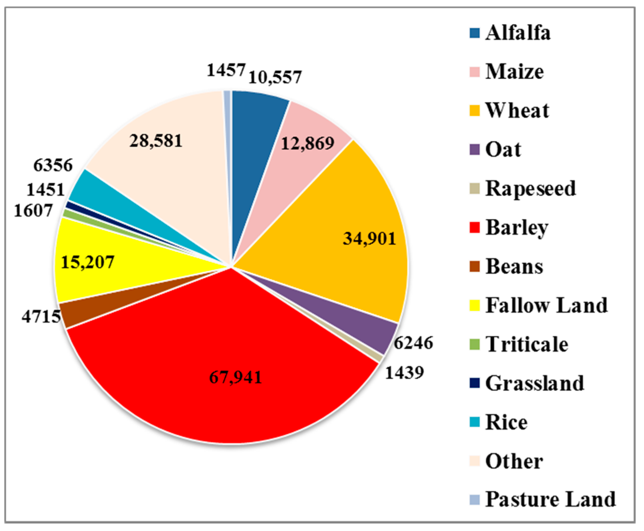
Remotesensing 11 01836 g002
Figure 3. Distribution of the number of agricultural plots per class of crop type.
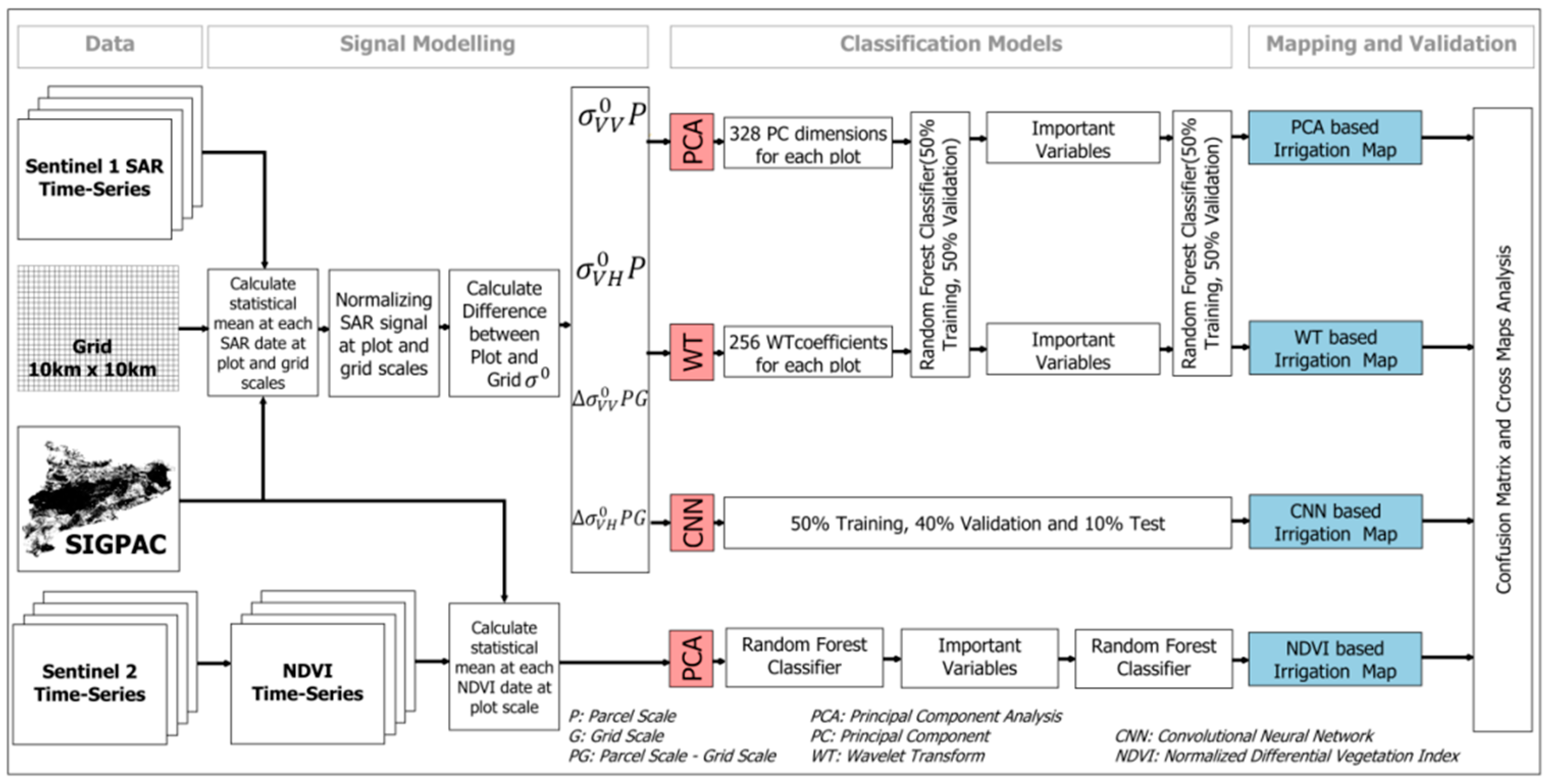
Remotesensing 11 01836 g003
Figure 4. Workflow overview using random forest (RF) and the convolutional neural network (CNN).
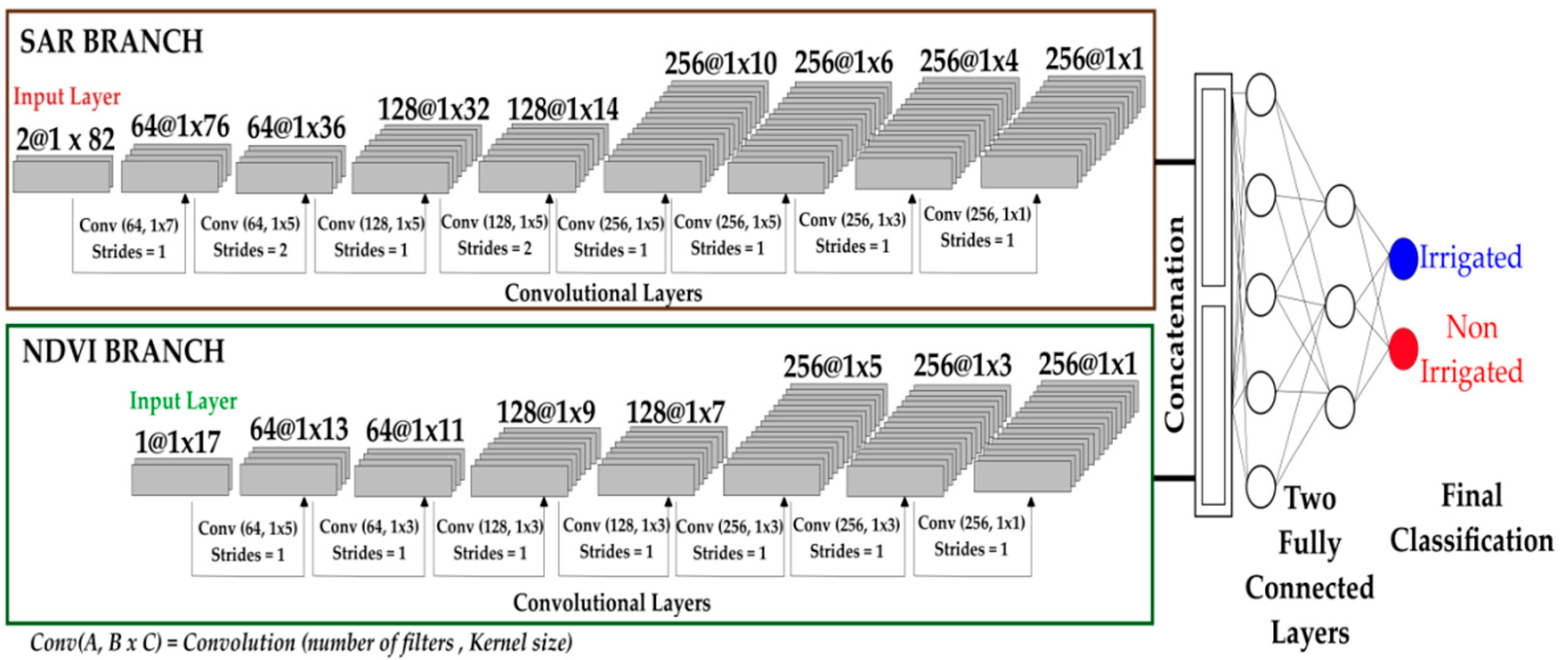
Remotesensing 11 01836 g004
Figure 5. Architecture of the one dimensional (1D) CNN model (CNN1D) used for classification of irrigated/non-irrigated plots using SAR and optical data.
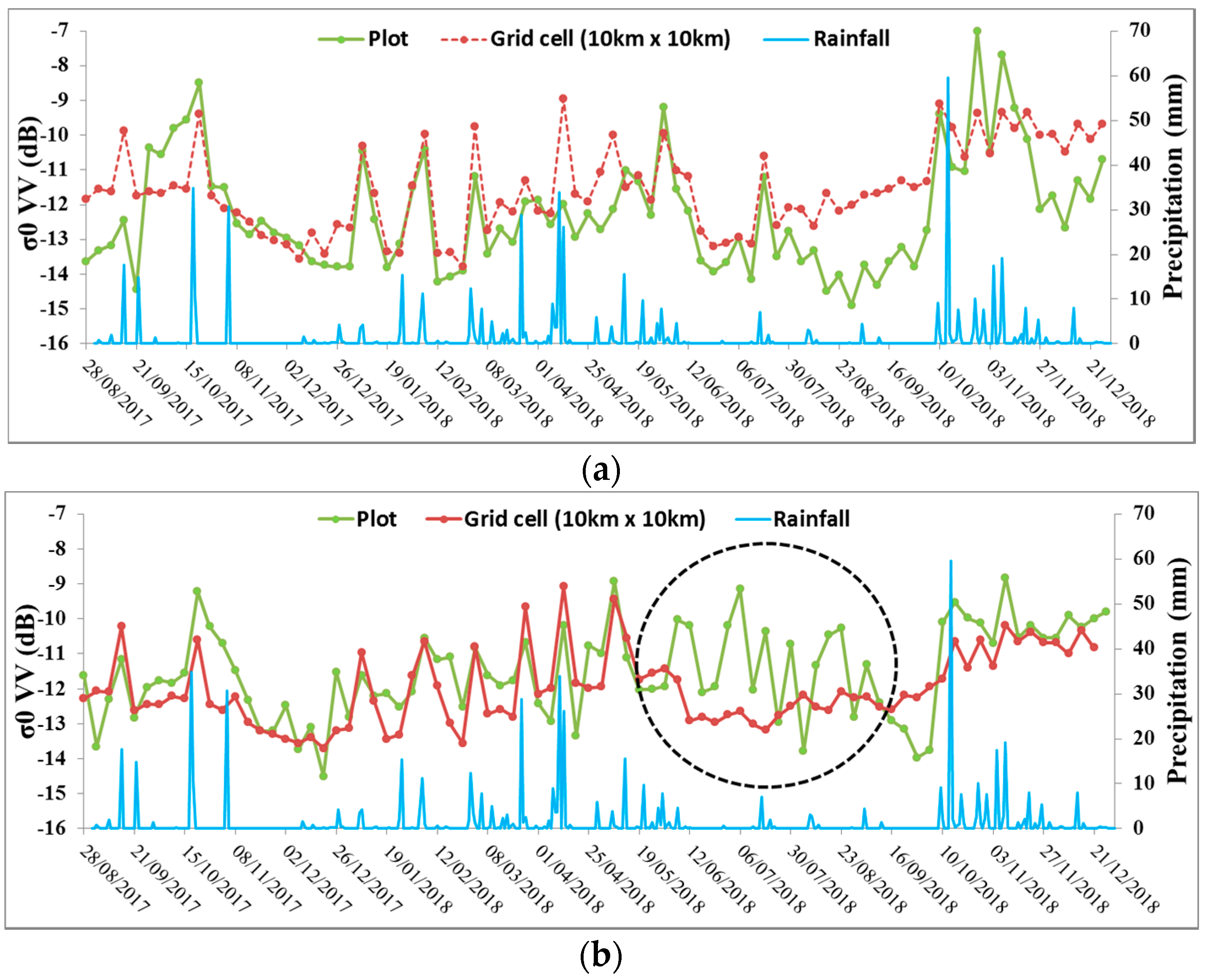
Remotesensing 11 01836 g005
Figure 6. Temporal evolution of SAR backscattering coefficient σ° in VV polarization at plot scale (green curve) and 10 km grid scale (red curve) with precipitation data recorded at a local meteorological station for (a) the non-irrigated plot, (b) the irrigated plot.
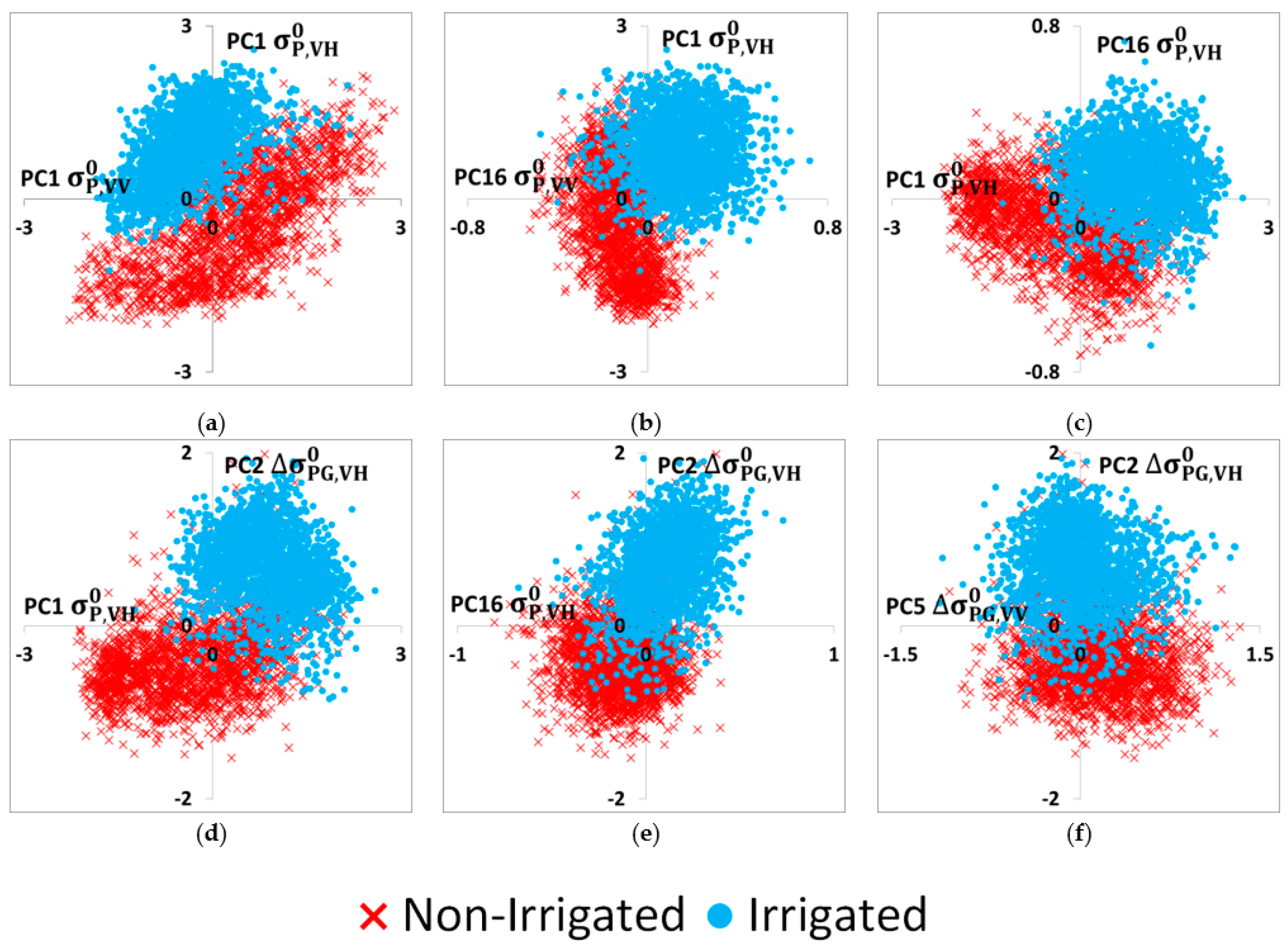
Remotesensing 11 01836 g006
Figure 7. Scatter plot of a random sample of 2000 irrigated and 2000 non-irrigated plots using different combinations of important principal component (PC) variables. Irrigated plots are presented in blue and non-irrigated plots represented in red. (a) PC1 of σ P , VV 0 with PC1 of σ P , VH 0 , (b) PC16 of σ P , VV 0 with PC1 of σ P , VH 0 , (c) PC1 of σ P , VH 0 with PC16 of σ P , VH 0 , (d) PC1 of σ P , VH 0 with PC2 of Δ σ PG , VV 0 , (e) PC16 of σ P , VH 0 with PC2 of Δ σ PG , VH 0   and (f) PC5 of Δ σ PG , VV 0 with PC2 of Δ σ PG , VV 0 . σ PG , VV 0   = σ P , VV 0 σ G , VV 0 and σ PG , VH 0   = σ P , VH 0 σ P , VH 0 . “P” means plot scale and “G” means grid scale.
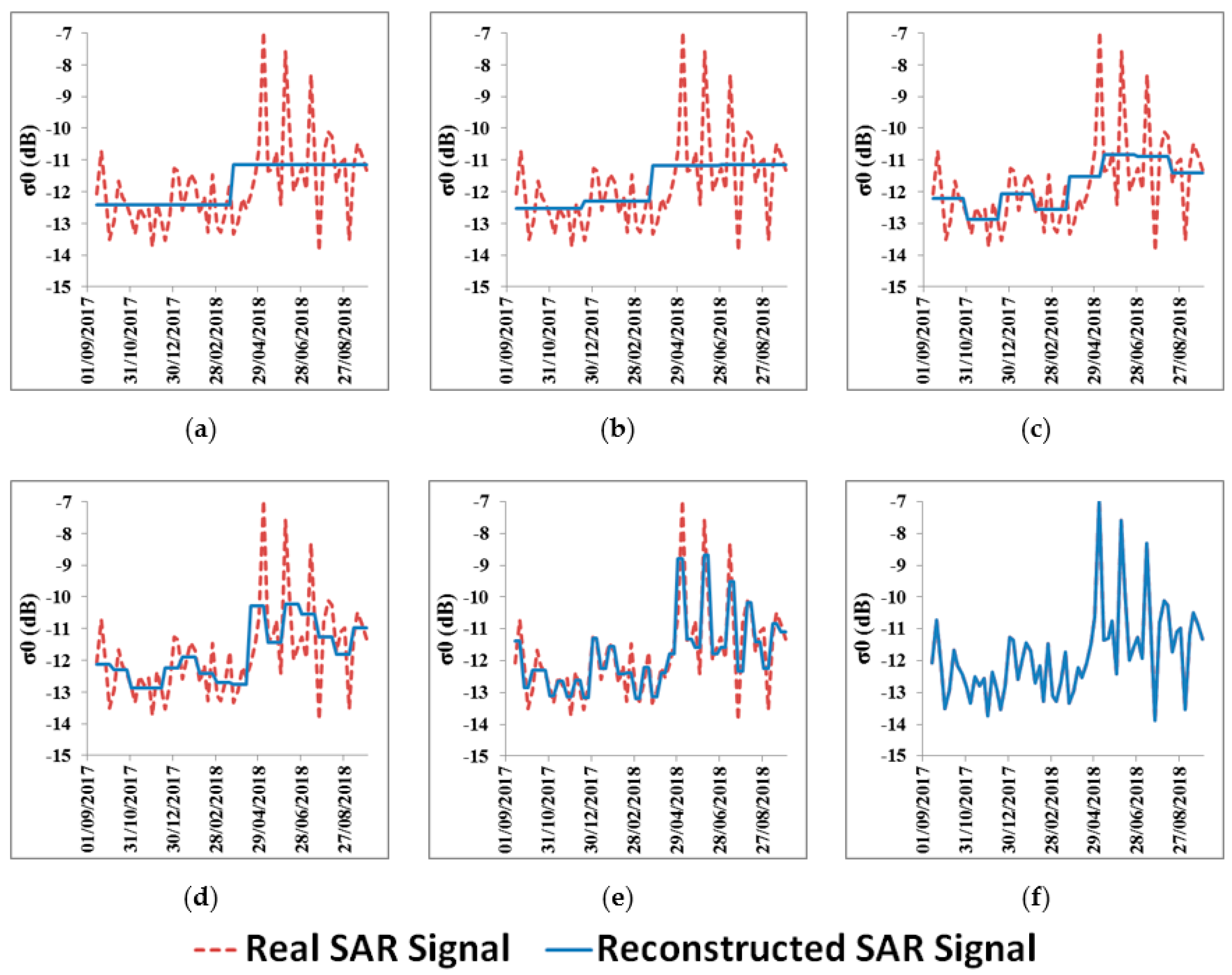
Remotesensing 11 01836 g007
Figure 8. Reconstruction of SAR signal in VV polarization at plot scale through the linear combinations of the ‘Haar’ wavelet coefficients using (a) 2 coefficients, (b) 4 coefficients, (c) 8 coefficients, (d) 16 coefficients, (e) 32 coefficients, and (f) 64 coefficients.
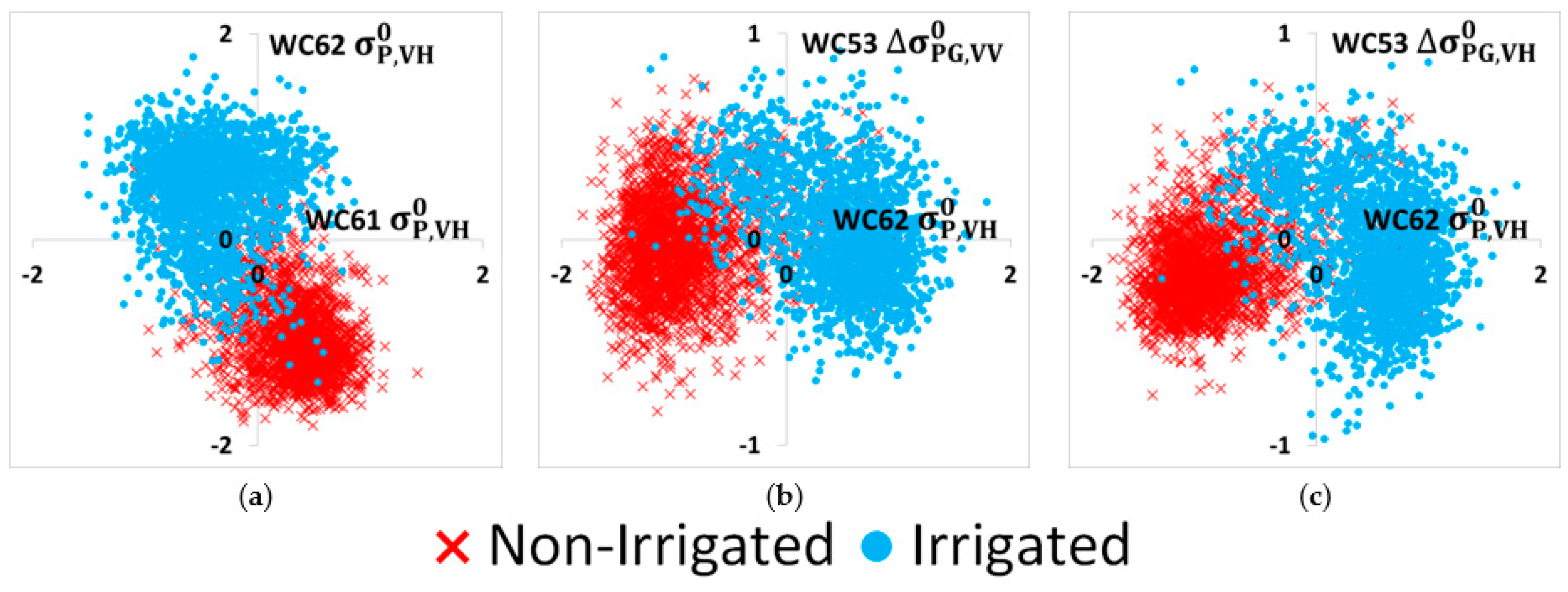
Remotesensing 11 01836 g008
Figure 9. Scatter plot of a random sample of 2000 irrigated and 2000 non-irrigated plots using different combinations of important wavelet transformation (WT) coefficients. Irrigated plots are presented in blue and non-irrigated plots represented in red (a) WC61 of σ P , VH 0 with WC62 of σ P , VH 0 , (b) WC62 of σ P , VH 0 with WC53 of Δ σ PG , VH 0 , (c) WC62 of σ P , VH 0 with WC53 of Δ σ PG , VH 0 . σ PG , VV 0 = σ P , VV 0 σ G , VV 0 and σ PG , VH 0 = σ P , VH 0 σ P , VH 0 . “P” means plot scale and “G” means grid scale and WC means wavelet coefficient.
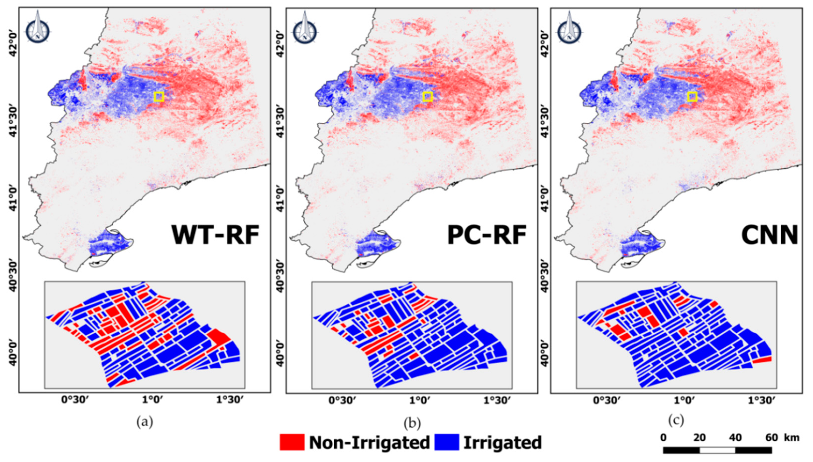
Remotesensing 11 01836 g009
Figure 10. Irrigation mapping using the (a) WT-RF model, (b) PC-RF model and (c) the CNN model. Irrigated areas are presented in blue while non-irrigated areas are shown in red. A zoom version of the yellow box in each map is provided to better visualize different classification results.
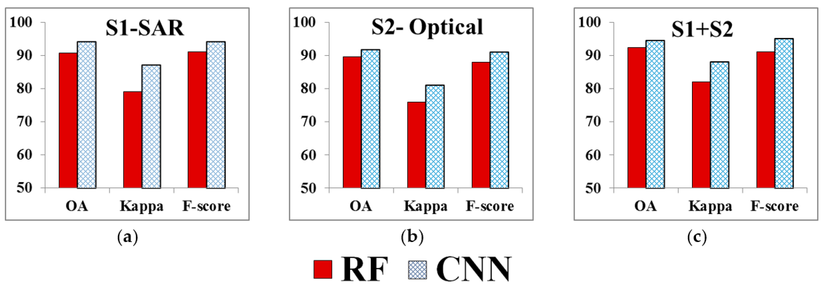
Remotesensing 11 01836 g010
Figure 11. Comparison of accuracy indices between RF and CNN classifications in three different scenarios: (a) Using the S1 SAR data, (b) using S2 optical data and (c) using S1 SAR and S2 optical data.
Remotesensing 11 01836 g011
Table 1. Summary of the used remote sensing data.
DataTypeSatelliteSpatial ResolutionImages NumberFrequency UsedCalibration PerformedBands Polarization
Satellite Images(Synthetic aperture radar) SARSentinel-110 m826 daysGeometric/Radiometric VV, VH
OpticalSentinel-210 m17One monthOrtho-rectified ReflectanceNear Infrared, Red
Table 2. Accuracy indices calculated for each classifier. TP is the number of the irrigated plots truly classified as irrigated, TN is the number non-irrigated plots truly classified as non-irrigated plots, FP is the number of non-irrigated plots falsely classified as irrigated, FN is the number of irrigated plots falsely classified as non-irrigated plots, N is the total number of plots, and EA is the expected accuracy.
IndexEquation
OA TP + TN TP + TN + FN + FP  
EA ( TP + FP ) × ( TP + FN ) + ( FN + TN ) × ( FP + TN ) ( TP + TN + FN + FP ) 2
Kappa OA EA 1 EA
F1 score 2 TP 2 TP + FP + FN
Precision TP TP + FP
Recall TP TP + FN
Table 3. The values of the overall accuracy, Kappa, F-score, precision, and recall obtained from the RF classifier using the 328 SAR PC variables and 15 important SAR PC variables.
MethodClassPrecisionRecallF-Score
PC-RF 328 VariablesIrrigated0.950.790.86
Non-Irrigated0.900.980.94
OA91.2%
Kappa0.79
F-score0.91
PC-RF 15 Important VariablesIrrigated0.920.810.86
Non-Irrigated0.900.960.93
OA90.7%
Kappa0.79
F-score0.91
Table 4. The values of the overall accuracy, Kappa, F-score, precision, and recall obtained from the RF classifier using the 256 wavelet coefficients and the 16 important wavelet coefficients.
MethodClassPrecisionRecallF-Score
WT-RF 256 VariablesIrrigated0.940.810.87
Non-Irrigated0.900.970.94
OA91.4%
Kappa0.81
F-score0.91
WT-RF 18 Important VariablesIrrigated0.890.780.83
Non-Irrigated0.890.950.92
OA89.1%
Kappa0.75
F-score0.89
Table 5. The values of the overall accuracy, Kappa, F-score, precision, and recall obtained from the RF classifier using the 17 normalized differential vegetation index (NDVI)-PC and the seven important NDVI PC values.
MethodClassPrecisionRecallF-Score
NDVI-RF 17 VariablesIrrigated0.940.780.85
Non-Irrigated0.890.970.93
OA90.5%
Kappa0.78
F-score0.91
NDVI-RF 7 Important VariablesIrrigated0.920.760.84
Non-Irrigated0.880.960.92
OA89.5%
Kappa0.76
F-score0.88
Table 6. The values of the overall accuracy, Kappa, F-score, precision, and recall obtained from the RF classifier using 15 important SAR PC variables and the seven important NDVI PC variables.
MethodClassPrecisionRecallF-Score
15 variable SAR PC-RF + 7 variable NDVI-RFIrrigated0.950.820.88
Non-Irrigated0.910.980.94
OA92.3%
Kappa0.82
F-score0.91
Table 7. The values of the overall accuracy, Kappa, F-score, precision, and recall obtained from the CNN method on SAR data.
MethodClassPrecisionRecallF-Score
CNN on SAR DataIrrigated0.930.890.91
Non-Irrigated0.950.960.96
OA94.1% ±   0.06
Kappa0.87 ±   0.0014
F-score0.94 ±   0.0006
Table 8. The values of the overall accuracy, Kappa, F-score, precision, and recall obtained from the CNN method on NDVI data.
MethodClassPrecisionRecallF-Score
CNN on Optical DataIrrigated0.930.810.87
Non-Irrigated0.910.970.94
OA91.6% ±   0.06
Kappa0.81 ±   0.0016
F-score0.91 ±   0.0006
Table 9. The values of the overall accuracy, Kappa, F-score, precision, and recall obtained from the CNN method on combined SAR and optical data.
MethodClassPrecisionRecallF-Score
CNN on Combined SAR and Optical DataIrrigated0.940.900.92
Non-Irrigated0.950.970.96
OA94.5% ± 0.05
Kappa0.88 ± 0.0016
F-score0.95 ± 0.0005

