Can we Monitor Height of Native Grasslands in Uruguay with Earth Observation?

 ,
,
Abstract
1. Introduction
2. Materials and Methods
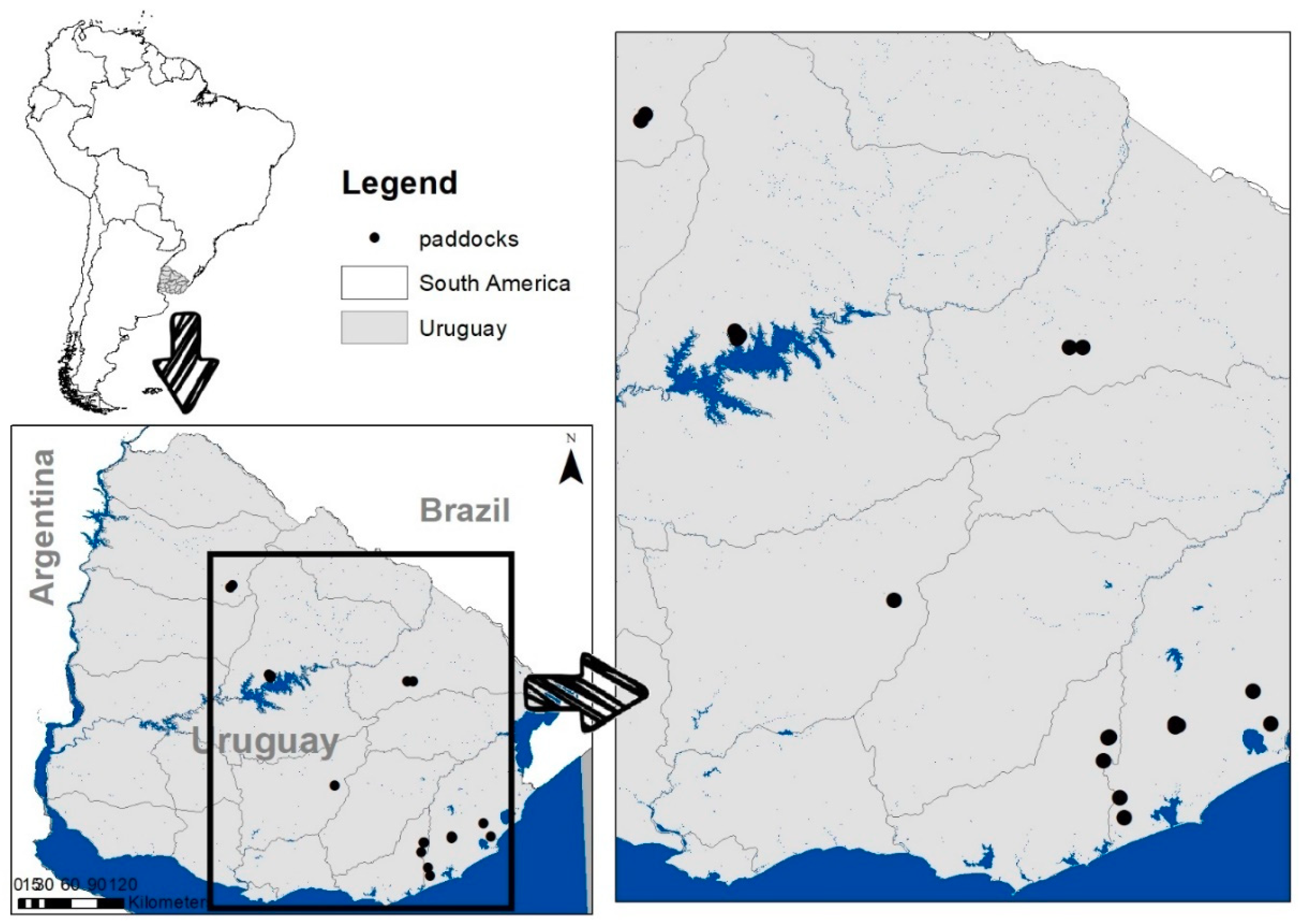
2.1. Study Area
2.2. Data
2.2.1. Farm Data
2.2.2. Satellite Data
Composite MODIS data
- MOD13Q1, 250 m V006 [35]. We selected the middle infrared band (MIR), near infrared band (NIR), and red bands; and the normalized difference vegetation index (NDVI) and enhanced vegetation index (EVI).
- MCD15A3H, 500 m V006 [36]. We used fraction of photosynthetically active radiation (FPAR) and leaf area index (LAI). According to Myneni et al. (2015), in this context and for this product, “LAI is defined as the one-sided green leaf area per unit ground area in broadleaf canopies and as one-half the total needle surface area per unit ground area in coniferous canopies. FPAR is defined as the fraction of incident photosynthetically active radiation (400–700 nm) absorbed by the green elements of a vegetation canopy”.
Daily MODIS data
- MOD09GQ (GQ). MODIS Terra/Aqua Surface Reflectance 250 m [37]. We selected the near infrared (NIR) and red bands; and estimated NDVI (NIR-Red/NIR+Red).
- MOD09GA (GA). MODIS Terra/Aqua Surface Reflectance 500 m. [37]. We selected MIR, NIR, and red bands; and estimated NDVI (NIR-red/NIR+red) and Normalized Difference Water Index, NDWI (NIR-MIR/NIR+MIR).
- MCD43A4 (Nbar). MODIS/Terra and Aqua Nadir BRDF (bidirectional reflectance distribution function) adjusted reflectance (NBAR), 500 m, V006 [38]. We selected MIR, NIR, and red bands; and estimated NDVI and NDWI.
Landsat data
2.2.3. Data Analysis
3. Results
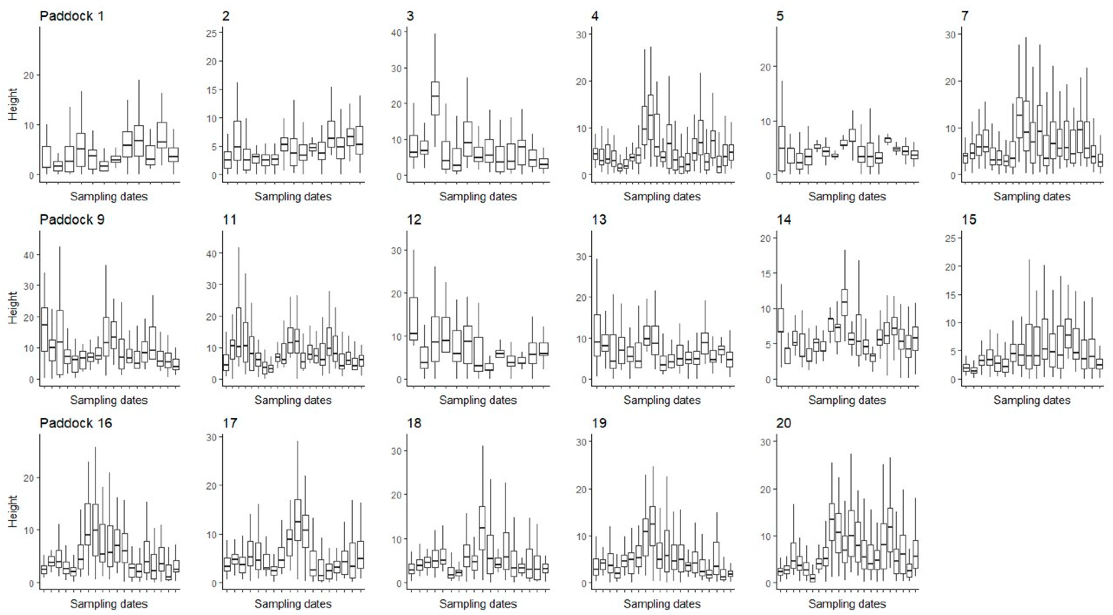
3.1. Farm Data
3.2. Composite MODIS Data
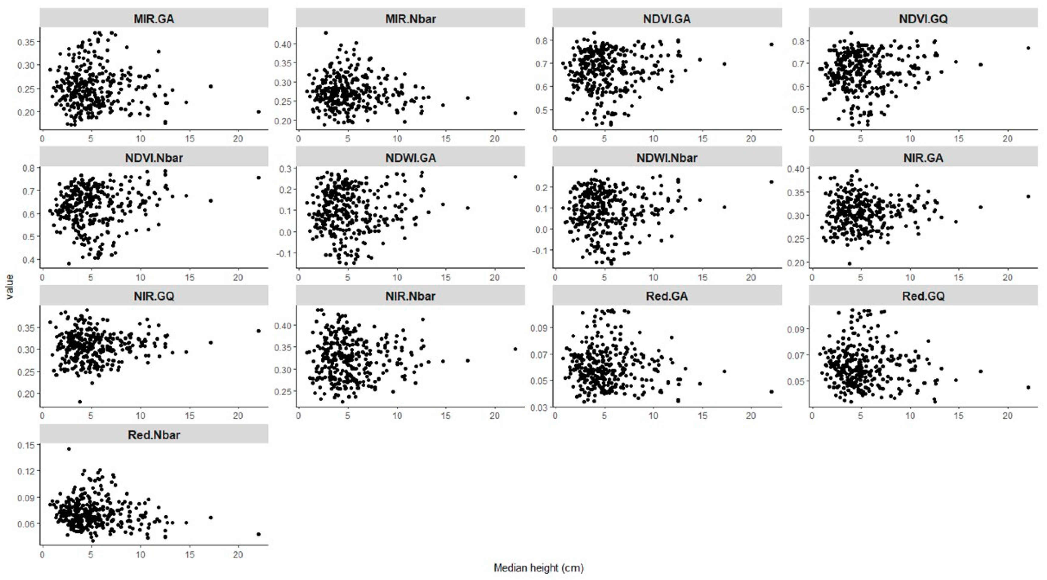
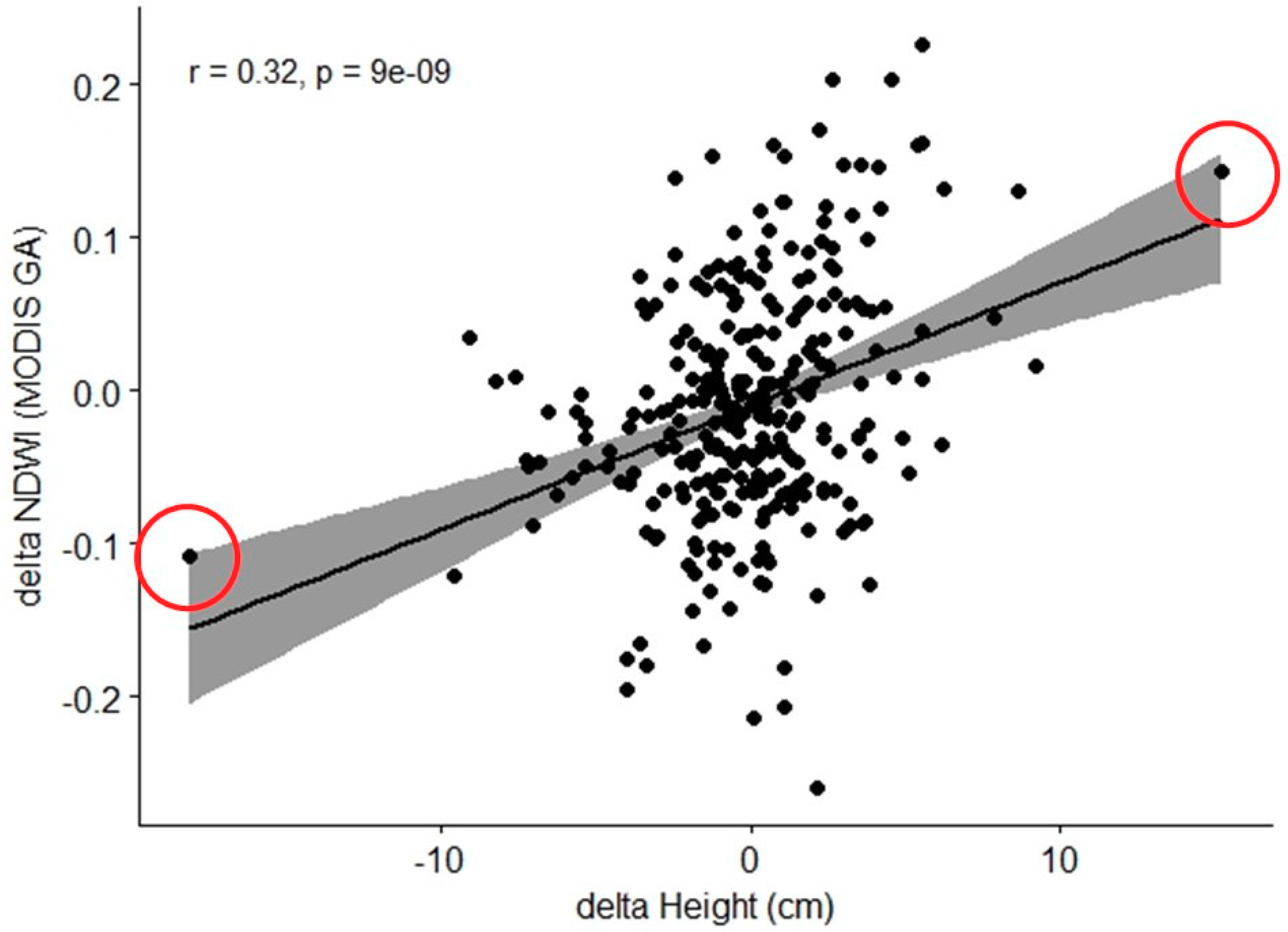
3.3. Daily MODIS Data
3.4. Variability
4. Discussion
5. Conclusions
Author Contributions
Funding
Acknowledgments
Conflicts of Interest
References
- Bilenca, D.; Miñarro, F. Identificación de Áreas Valiosas de Pastizal en las Pampas y Campos de Argentina, Uruguay y Sur de Brasil, 1st ed.; Fundación Vida Silvestre Argentina: Buenos Aires, Argentina, 2004; ISBN 950942711X. [Google Scholar]
- Suttie, J.M.; Reynolds, S.G.; Batello, C. Grasslands of the World; Food and Agriculture Organization: Rome, Italy, 2005; ISBN 9251053375. [Google Scholar]
- Allen, V.G.; Batello, C.; Berretta, E.J.; Hodgson, J.; Kothmann, M.; Li, X.; McIvor, J.; Milne, J.; Morris, C.; Peeters, A.; et al. An international terminology for grazing lands and grazing animals. Grass Forage Sci. 2011, 66, 2–28. [Google Scholar] [CrossRef]
- Sala, O.E.; Paruelo, J.M. Ecosystem service in grasslands. In Nature´s Services: Societal Dependence on Natural Ecosystems; Daily, G., Ed.; Island Press: Washington, DC, USA, 1995; Volume 92, pp. 237–252. ISBN 9780465022342. [Google Scholar]
- O’Mara, F.P. The role of grasslands in food security and climate change. Ann. Bot. 2012, 110, 1263–1270. [Google Scholar] [CrossRef] [PubMed]
- Soriano, A. Temperate subhumid grasslands of South America. In Ecosyst. WorldTemperate subhumid grasslands; Coupland, R.T., Ed.; Natural Grasslands.. Elsevier Scientific Publishing Company: Amsterdam, the Netherlands, 1991; Volume 8A, pp. 367–407. [Google Scholar]
- Berretta, E.; Risso, D.; Montossi, F.; Pigurina, G. Campos in Uruguay. In Grassland Ecophysiology and Grazing, 1st ed.; CABI Publishing: New York, NY, USA, 2000; pp. 377–394. [Google Scholar]
- Rosengurtt, B. Estudios Sobre Praderas Naturales del Uruguay: 3 Contribución; Casa Barreiro y Ramos: Montevideo, Uruguay, 1943. [Google Scholar]
- Altesor, A.; Pezzani, F. Relationship between spatial strategies and morphological attributes in a Uruguayan grassland: A functional approach. J. Veg. Sci. 1999, 10, 457–462. [Google Scholar] [CrossRef]
- Boggiano, P.; Berretta, E. Factores que afectan la biodiversidad del campo natural. 21 Reun. do Grup. Técnico em Forrageiras do Cone Sul Grup. Campos 2006, 1, 93–104. [Google Scholar]
- Wheeler, J.L.; Burns, J.C.; Mochrie, R.D.; Gross, H.D. The choice of fixed or variable stocking rates in grazing experiments. Exp. Agric. 1973, 9, 289–302. [Google Scholar] [CrossRef]
- Aiken, G.E. Invited Review: Grazing management options in meeting objectives of grazing experiments12. Prof. Anim. Sci. 2016, 32, 1–9. [Google Scholar] [CrossRef]
- Mott, G.O. Grazing pressure and the measurement of pasture production. In Proceedings of the Grazing Management, 8th International Grasslands Congress, Reading, UK, 11–21 July 1960; pp. 606–611. [Google Scholar]
- Sollenberger, L.E.; Moore, J.E.; Allen, V.G.; Pedreira, C.G.S. Reporting forage allowance in grazing experiments. Crop Sci. 2005, 45, 896–900. [Google Scholar] [CrossRef]
- Do Carmo, M.; Sollenberger, L.E.; Carriquiry, M.; Soca, P. Controlling herbage allowance and selection of cow genotype improve cow-calf productivity in Campos grasslands. Prof. Anim. Sci. 2018, 34, 32–41. [Google Scholar] [CrossRef]
- Do Carmo, M.; Cardozo, G.; Ruggia, A.; Soca, P. Prediction of herbage mass in Campos grassland based on herbage height. In Proceedings of the 10th International Symposium on the Nutrition of Herbivoresdvances, Clermont-Ferrand, France, 2–6 September 2018; p. 418. [Google Scholar]
- Wachendorf, M.; Fricke, T.; Möckel, T. Remote sensing as a tool to assess botanical composition, structure, quantity and quality of temperate grasslands. Grass Forage Sci. 2017, 73, 1–14. [Google Scholar] [CrossRef]
- Lawley, V.; Lewis, M.; Clarke, K.; Ostendorf, B. Site-based and remote sensing methods for monitoring indicators of vegetation condition: An Australian review. Ecol. Indic. 2016, 60, 1273–1283. [Google Scholar] [CrossRef]
- Baeza, S.; Lezama, F. Spatial variability of above-ground net primary production in Uruguayan grasslands: A remote sensing approach. Appl. Veg. 2010, 13, 72–85. [Google Scholar] [CrossRef]
- Baldassini, P.; Volante, J.N.J.N.; Califano, L.M.; Paurelo, J.M. Caracterización regional de la estructura y de la productividad de la vegetación de la Puna mediante el uso de imágenes MODIS. Ecol. Austral 2012, 22, 22–32. [Google Scholar]
- Guerschman, J.P.; Paruelo, J.M.; Di Bella, C.; Giallorenzi, M.C.; Pacin, F. Land cover classification in the Argentine Pampas using multi-temporal Landsat TM data. Int. J. Remote Sens. 2003, 24, 3381–3402. [Google Scholar] [CrossRef]
- Piñeiro, G.; Oesterheld, M.; Paruelo, J.M. Seasonal Variation in Aboveground Production and Radiation-use Efficiency of Temperate rangelands Estimated through Remote Sensing. Ecosystems 2006, 9, 357–373. [Google Scholar] [CrossRef]
- An, N.; Price, K.P.; Blair, J.M. Estimating above-ground net primary productivity of the tallgrass prairie ecosystem of the Central Great Plains using AVHRR NDVI. Int. J. Remote Sens. 2013, 34, 3717–3735. [Google Scholar] [CrossRef]
- Li, F.; Zeng, Y.; Luo, J.; Ma, R.; Wu, B. Modeling grassland aboveground biomass using a pure vegetation index. Ecol. Indic. 2016, 62, 279–288. [Google Scholar] [CrossRef]
- Jia, W.; Liu, M.; Yang, Y.; He, H.; Zhu, X.; Yang, F.; Yin, C.; Xiang, W. Estimation and uncertainty analyses of grassland biomass in Northern China: Comparison of multiple remote sensing data sources and modeling approaches. Ecol. Indic. 2016, 60, 1031–1040. [Google Scholar] [CrossRef]
- Olsen, J.L.; Miehe, S.; Ceccato, P.; Fensholt, R. Does EO NDVI seasonal metrics capture variations in species composition and biomass due to grazing in semi-arid grassland savannas? Biogeosciences 2015, 12, 4407–4419. [Google Scholar] [CrossRef]
- Gaitán, J.J.; Bran, D.; Oliva, G.; Ciari, G.; Nakamatsu, V.; Salomone, J.; Ferrante, D.; Buono, G.; Massara, V.; Humano, G.; et al. Evaluating the performance of multiple remote sensing indices to predict the spatial variability of ecosystem structure and functioning in Patagonian steppes. Ecol. Indic. 2013, 34, 181–191. [Google Scholar] [CrossRef]
- Marsett, R.R.C.R.; Qi, J.; Heilman, P.; Biedenbender, S.H.; Watson, M.C.; Amer, S.; Weltz, M.; Goodrich, D.; Marsett, R.R.C.R. Remote Sensing for Grassland Management in the Arid Southwest. Rangel. Ecol. Manag. 2006, 59, 530–540. [Google Scholar] [CrossRef]
- Ali, I.; Cawkwell, F.; Dwyer, E.; Barrett, B.; Green, S. Satellite remote sensing of grasslands: From observation to management. J. Plant Ecol. 2016, 9, 649–671. [Google Scholar] [CrossRef]
- Cimbelli, A.; Vitale, V. Grassland Height Assessment by Satellite Images. Adv. Remote Sens. 2017, 6, 40–53. [Google Scholar] [CrossRef]
- Crabbe, R.A.; Lamb, D.W. Estimating Biophysical Variables of Pasture Cover Using Sentinel-1 Data; Precision Agriculture NZ Inc.: Christchurch, New Zealand, 2017; pp. 1–8. [Google Scholar]
- Crabbe, R.A.; Lamb, D.W.; Edwards, C.; Andersson, K.; Schneider, D. A Preliminary Investigation of the Potential of Sentinel-1 Radar to Estimate Pasture Biomass in a Grazed, Native Pasture Landscape. Remote Sens. 2019, 11, 872. [Google Scholar] [CrossRef]
- Haydock, K.P.; Shaw, N.H. The comparitive yield method for estimating dry matter yield of pasture. Aust. J. Exp. Agric. 1975, 15, 663–670. [Google Scholar]
- Duveiller, G.; Defourny, P. A conceptual framework to de fi ne the spatial resolution requirements for agricultural monitoring using remote sensing. Remote Sens. Environ. 2010, 114, 2637–2650. [Google Scholar] [CrossRef]
- Didan, K. MOD13Q1 MODIS/Terra Vegetation Indices 16-Day L3 Global 250m SIN Grid V006 [Data Set]. 2015. Available online: https://search.earthdata.nasa.gov/search (accessed on 1 October 2017).
- Myneni, R.; Knyazikhin, Y.; Park, T. MCD15A3H MODIS/Terra+Aqua Leaf Area Index/FPAR 4-day L4 Global 500 m SIN Grid V006 [Data Set]. 2015. Available online: https://search.earthdata.nasa.gov/search (accessed on 1 October 2017).
- Vermote, E.F.; Roger, J.C.; Ray, J.P. MODIS Surface Reflectance User’s Guide collection 6. MODIS L. Surf. Reflectance Sci. Comput. Facil 2015, 1–36. [Google Scholar]
- Schaaf, C.; Wang, Z. MCD43A4 MODIS/Terra+Aqua BRDF/Albedo Nadir BRDF Adjusted Ref Daily L3 Global-500m V006 [Data Set]. NASA EOSDIS Land Processes DAAC. 2015. Available online: https://search.earthdata.nasa.gov/search (accessed on 1 October 2017).
- The United States Geological Survey. Product Guide LANDSAT 8 Surface Reflectance Code (LASRC) Product; Version 2.0; EROS: Sioux Falls, SD, USA, 2018.
- Laca, E.A.; Demment, M.W.; Winckel, J.; Kie, J.G. Comparison of weight estimate and rising-plate meter methods to measure herbage mass of a mountain meadow. J. Range Manag. 1989, 42, 71–75. [Google Scholar] [CrossRef]
- Payero, J.O.; Neale, C.M.U.; Wright, J.L. Comparision of eleven vegetation indices for estimating plant height of alfalfa and grass. Appl. Eng. Agric. 2004, 20, 385–394. [Google Scholar] [CrossRef]
- INIA (GRAS) NDVI Nacional Monitoring. Available online: http://www.inia.uy/gras/Monitoreo-Ambiental/Monitoreo-de-la-vegetación (accessed on 1 April 2019).
- d’Andrimont, R.; Lemoine, G.; Velde, M. Targeted Grassland Monitoring at Parcel Level Using Sentinels, Street-Level Images and Field Observations. Remote Sens. 2018, 10, 1300. [Google Scholar] [CrossRef]
- Wood, E.M.; Pidgeon, A.M.; Radeloff, V.C.; Keuler, N.S. Image texture as a remotely sensed measure of vegetation structure. Remote Sens. Environ. 2012, 121, 516–526. [Google Scholar] [CrossRef]
- Zalite, K. Radar Remote Sensing for Monitoring Forest Floods and Agricultural Grasslands; University of Tartu Press: Tartu, Estonia, 2016; ISBN 978-9949-77-025-0. [Google Scholar]
- Tamm, T.; Zalite, K.; Voormansik, K.; Talgre, L. Relating Sentinel-1 Interferometric Coherence to Mowing Events on Grasslands. Remote Sens. 2016, 8, 802. [Google Scholar] [CrossRef]
- López-Díaz, J.E.; González-Rodríguez, A. Measuring Herbage Mass by Non-Destructive Methods: A Review. J. Agric. Sci. Technol. 2011, 1, 303–314. [Google Scholar]
- Grüner, E.; Astor, T.; Wachendorf, M. Biomass Prediction of Heterogeneous Temperate Grasslands Using an SfM Approach Based on UAV Imaging. Agronomy 2019, 9, 54. [Google Scholar] [CrossRef]


| Paddock Number | Area (has) |
|---|---|
| 3(B), 4(A), 7(C), 9(E), 10 (E), 19(D), 20(F) | 12–50 |
| 8 (E), 11 (E), 15 (G), 16 (G), 17 (H), 18 (H) | 51–100 |
| 1 (I), 2 (I), 5 (K), 12 (E), 13 (E), 14(J) | 101–150 |
| 6 (K) | >151 |
| P | FPAR | LAI | MIR | NIR | Red | NDVI | EVI |
|---|---|---|---|---|---|---|---|
| 1 | 0.024 | 0.204 | 0.335 | 0.041 | 0.248 | 0.201 | 0.141 |
| 2 | 0.084 | 0.013 | 0.355 | 0.042 | 0.306 | 0.244 | 0.200 |
| 3 | 0.217 | 0.305 | 0.606 | 0.173 | 0.514 | 0.428 | 0.307 |
| 4 | 0.605 | 0.376 | 0.030 | 0.290 | 0.087 | 0.076 | 0.246 |
| 5 | 0.324 | 0.458 | 0.182 | 0.289 | 0.305 | 0.354 | 0.349 |
| 7 | 0.180 | 0.225 | 0.094 | 0.079 | 0.146 | 0.029 | 0.067 |
| 9 | 0.603 | 0.468 | 0.537 | 0.306 | 0.481 | 0.571 | 0.543 |
| 11 | 0.555 | 0.363 | 0.499 | 0.253 | 0.323 | 0.411 | 0.390 |
| 12 | 0.076 | 0.036 | 0.091 | 0.228 | 0.119 | 0.043 | 0.042 |
| 13 | 0.444 | 0.274 | 0.402 | 0.229 | 0.387 | 0.409 | 0.406 |
| 14 | 0.247 | 0.263 | 0.471 | 0.285 | 0.324 | 0.351 | 0.353 |
| 15 | 0.328 | 0.250 | 0.407 | 0.188 | 0.380 | 0.240 | 0.001 |
| 16 | 0.235 | 0.237 | 0.728 | 0.059 | 0.528 | 0.490 | 0.306 |
| 17 | 0.478 | 0.282 | 0.400 | 0.065 | 0.130 | 0.370 | 0.335 |
| 18 | 0.574 | 0.390 | 0.003 | 0.098 | 0.571 | 0.261 | 0.002 |
| 19 | 0.447 | 0.363 | 0.163 | 0.483 | 0.190 | 0.543 | 0.588 |
| 20 | 0.367 | 0.282 | 0.218 | 0.063 | 0.131 | 0.083 | 0.018 |
| H Median | H Average | H Mode | H Maximum | |
|---|---|---|---|---|
| MIR (GA product) | 0.032 | 0.018 | 0.013 | 0.034 |
| NIR (GA product) | 0.090 | 0.070 | 0.003 | 0.036 |
| Red (GA product) | 0.085 | 0.067 | 0.041 | 0.008 |
| NDVI (GA product) | 0.108 | 0.087 | 0.037 | 0.012 |
| NDWI (GA product) | 0.079 | 0.058 | 0.013 | 0.002 |
| NIR (GQ product) | 0.083 | 0.058 | 0.009 | 0.029 |
| Red (GQ product) | 0.092 | 0.077 | 0.047 | 0.001 |
| NDVI (GQ product) | 0.112 | 0.092 | 0.047 | 0.016 |
| MIR (Nbar product) | 0.087 | 0.092 | 0.008 | 0.056 |
| NIR (Nbar product) | 0.014 | 0.011 | 0.000 | 0.051 |
| Red (Nbar product) | 0.163 | 0.156 | 0.070 | 0.092 |
| NDVI (Nbar product) | 0.136 | 0.121 | 0.060 | 0.051 |
| NDWI (Nbar product) | 0.081 | 0.070 | 0.011 | 0.016 |
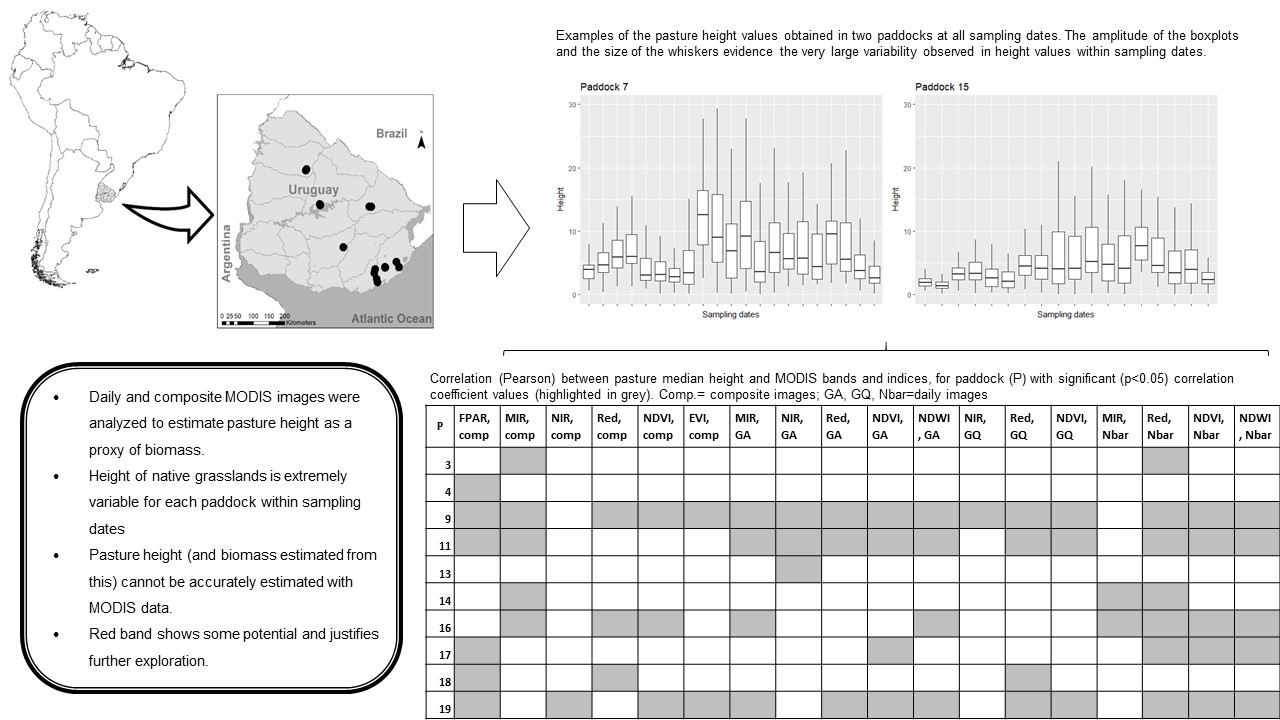
| P | MIR, GA | NIR, GA | Red, GA | NDVI, GA | NDWI, GA | NIR, GQ | Red, GQ | NDVI, GQ | MIR, Nbar | NIR, Nbar | Red, Nbar | NDVI, Nbar | NDWI, Nbar |
|---|---|---|---|---|---|---|---|---|---|---|---|---|---|
| 1 | 0.002 | 0.074 | 0.010 | 0.003 | 0.027 | 0.036 | 0.029 | 0.021 | 0.008 | 0.039 | 0.001 | 0.000 | 0.014 |
| 2 | 0.246 | 0.122 | 0.002 | 0.039 | 0.105 | 0.135 | 0.012 | 0.052 | 0.214 | −0.323 | 0.161 | 0.015 | −0.020 |
| 3 | 0.525 | 0.314 | 0.431 | 0.377 | 0.522 | 0.361 | 0.333 | 0.329 | 0.539 | 0.139 | 0.645 | 0.500 | 0.492 |
| 4 | 0.036 | 0.014 | 0.014 | 0.001 | 0.036 | 0.018 | 0.080 | 0.069 | 0.062 | 0.028 | 0.174 | 0.168 | 0.019 |
| 5 | 0.256 | 0.383 | 0.429 | 0.464 | 0.372 | 0.377 | 0.429 | 0.441 | 0.067 | 0.362 | 0.309 | 0.432 | 0.359 |
| 7 | 0.180 | 0.258 | 0.342 | 0.352 | 0.290 | 0.229 | 0.293 | 0.323 | 0.071 | 0.137 | −0.283 | 0.225 | 0.081 |
| 9 | 0.546 | 0.519 | 0.574 | 0.615 | 0.679 | 0.479 | 0.558 | 0.597 | 0.438 | 0.460 | 0.547 | 0.619 | 0.600 |
| 11 | 0.453 | 0.450 | 0.467 | 0.494 | 0.520 | 0.386 | 0.445 | 0.466 | 0.349 | 0.422 | 0.445 | 0.530 | 0.509 |
| 12 | 0.115 | 0.074 | 0.140 | 0.106 | 0.062 | 0.022 | 0.166 | −0.140 | 0.120 | 0.002 | 0.040 | 0.031 | 0.103 |
| 13 | 0.116 | 0.523 | 0.136 | 0.246 | 0.334 | 0.481 | 0.159 | 0.263 | 0.358 | 0.192 | −0.420 | 0.397 | 0.397 |
| 14 | 0.288 | 0.276 | 0.252 | 0.277 | 0.323 | 0.280 | 0.226 | 0.261 | 0.519 | 0.015 | 0.511 | 0.327 | 0.309 |
| 15 | 0.425 | 0.160 | 0.472 | 0.257 | 0.136 | 0.121 | 0.301 | 0.167 | 0.262 | 0.002 | 0.351 | 0.212 | 0.192 |
| 16 | 0.482 | 0.371 | 0.272 | 0.364 | 0.499 | 0.366 | 0.221 | 0.315 | 0.579 | 0.160 | 0.607 | 0.533 | 0.576 |
| 17 | 0.335 | 0.295 | 0.390 | 0.469 | 0.430 | 0.283 | 0.367 | 0.444 | 0.172 | 0.202 | 0.576 | 0.609 | 0.504 |
| 18 | 0.268 | 0.211 | 0.447 | 0.408 | 0.288 | 0.204 | 0.475 | 0.415 | 0.278 | 0.051 | 0.420 | 0.353 | 0.342 |
| 19 | 0.482 | 0.351 | 0.555 | 0.523 | 0.501 | 0.328 | 0.610 | 0.556 | 0.257 | 0.250 | 0.594 | 0.584 | 0.467 |
| 20 | 0.061 | 0.241 | 0.053 | 0.097 | 0.059 | 0.162 | 0.020 | 0.052 | 0.266 | 0.346 | 0.268 | 0.008 | 0.106 |
| P | MIR, GA | NIR, GA | Red, GA | NDVI, GA | NDWI, GA | NIR, GQ | Red, GQ | NDVI, GQ | MIR, Nbar | NIR, Nbar | Red, Nbar | NDVI, Nbar | NDWI, Nbar |
|---|---|---|---|---|---|---|---|---|---|---|---|---|---|
| 1 | 0.316 | 0.479 | 0.323 | 0.457 | 0.514 | 0.522 | 0.339 | 0.476 | 0.305 | 0.412 | 0.283 | 0.410 | 0.510 |
| 2 | 0.093 | 0.597 | 0.380 | 0.458 | 0.379 | 0.568 | 0.373 | 0.463 | 0.470 | 0.031 | 0.419 | 0.379 | 0.385 |
| 3 | 0.591 | 0.201 | 0.541 | 0.392 | 0.637 | 0.242 | 0.408 | 0.336 | 0.499 | 0.106 | 0.604 | 0.500 | 0.550 |
| 4 | 0.134 | 0.092 | 0.205 | 0.194 | 0.143 | 0.138 | 0.216 | 0.224 | 0.001 | 0.267 | 0.331 | 0.386 | 0.158 |
| 5 | 0.223 | 0.518 | 0.314 | 0.462 | 0.493 | 0.552 | 0.336 | 0.462 | 0.291 | 0.386 | 0.392 | 0.527 | 0.540 |
| 7 | 0.009 | 0.051 | 0.183 | 0.188 | 0.047 | 0.010 | 0.093 | 0.110 | 0.319 | 0.027 | 0.106 | 0.125 | 0.317 |
| 9 | 0.225 | 0.480 | 0.301 | 0.403 | 0.490 | 0.447 | 0.281 | 0.380 | 0.255 | 0.320 | 0.342 | 0.378 | 0.348 |
| 11 | 0.108 | 0.506 | 0.266 | 0.374 | 0.361 | 0.467 | 0.258 | 0.364 | 0.254 | 0.305 | 0.342 | 0.377 | 0.329 |
| 12 | 0.072 | 0.251 | 0.154 | 0.189 | 0.195 | 0.217 | 0.139 | 0.172 | 0.015 | 0.296 | 0.272 | 0.302 | 0.145 |
| 13 | 0.425 | 0.501 | 0.444 | 0.532 | 0.666 | 0.485 | 0.482 | 0.567 | 0.632 | 0.366 | 0.623 | 0.629 | 0.706 |
| 14 | 0.063 | 0.404 | 0.173 | 0.281 | 0.258 | 0.367 | 0.108 | 0.218 | 0.260 | 0.045 | 0.389 | 0.279 | 0.135 |
| 15 | 0.603 | 0.019 | 0.293 | 0.232 | 0.348 | 0.056 | 0.176 | 0.167 | 0.223 | 0.084 | 0.022 | 0.076 | 0.270 |
| 16 | 0.173 | 0.240 | 0.132 | 0.190 | 0.293 | 0.277 | 0.147 | 0.205 | 0.143 | 0.186 | 0.254 | 0.355 | 0.370 |
| 17 | 0.181 | 0.300 | 0.282 | 0.406 | 0.351 | 0.251 | 0.306 | 0.409 | 0.065 | 0.301 | 0.371 | 0.539 | 0.477 |
| 18 | 0.153 | 0.369 | 0.221 | 0.296 | 0.329 | 0.388 | 0.260 | 0.323 | 0.050 | 0.114 | 0.248 | 0.267 | 0.188 |
| 19 | 0.038 | 0.160 | 0.320 | 0.296 | 0.133 | 0.205 | 0.350 | 0.353 | 0.158 | 0.286 | 0.148 | 0.363 | 0.232 |
| 20 | 0.094 | 0.075 | 0.007 | 0.012 | 0.114 | 0.145 | 0.046 | 0.064 | 0.256 | 0.105 | 0.293 | 0.145 | 0.077 |
| P | Dates Considered | Landsat | MODIS GQ | MODIS Comp | MODIS GA | ||||
|---|---|---|---|---|---|---|---|---|---|
| CV | SD | CV | SD | CV | SD | CV | SD | ||
| 1 | 10 | 12.04 | 1.44 | 6.27 | 0.95 | 6.23 | 0.83 | 5.89 | 2.15 |
| 2 | 12 | 9.89 | 4.05 | 4.41 | 6.59 | 4.49 | 2.59 | 1.56 | 0.58 |
| 3 | 8 | 15.32 | 13.12 | 2.92 | 1.74 | 4.15 | 1.70 | 2.88 | 0.86 |
| 4 | 9 | 10.89 | 3.27 | 5.01 | 6.75 | 5.38 | 1.78 | ||
| 5 | 9 | 18.10 | 10.67 | 8.64 | 1.67 | 11.43 | 5.11 | 6.87 | 3.52 |
| 6 | 4 | 11.95 | 11.49 | 9.18 | 2.07 | 8.09 | 2.45 | 8.89 | 2.55 |
| 7 | 10 | 15.95 | 6.78 | 4.86 | 1.66 | 4.75 | 1.18 | ||
| 8 | 8 | 8.43 | 3.08 | 4.23 | 2.10 | 5.64 | 1.37 | 9.50 | 8.66 |
| 9 | 12 | 9.94 | 7.33 | 3.15 | 1.78 | 3.56 | 1.56 | 2.16 | 1.63 |
| 10 | 2 | 4.76 | 1.06 | 1.62 | 0.27 | 2.21 | 0.09 | ||
| 11 | 13 | 7.79 | 2.34 | 3.27 | 1.53 | 4.03 | 2.19 | 2.04 | 1.24 |
| 12 | 11 | 8.95 | 1.88 | 2.60 | 1.28 | 4.72 | 2.08 | 1.35 | 0.93 |
| 13 | 14 | 8.63 | 2.86 | 3.22 | 1.10 | 5.09 | 1.93 | 3.23 | 1.10 |
| 14 | 14 | 14.98 | 7.45 | 7.07 | 3.20 | 7.74 | 2.75 | 4.01 | 3.93 |
| 15 | 11 | 18.44 | 11.39 | 3.96 | 1.04 | 4.52 | 0.76 | 2.86 | 1.85 |
| 16 | 12 | 14.78 | 4.68 | 6.51 | 1.37 | 6.71 | 1.67 | 6.00 | 2.04 |
| 17 | 6 | 14.12 | 8.52 | 5.71 | 3.60 | 8.96 | 5.75 | 4.52 | 2.51 |
| 18 | 6 | 11.94 | 6.12 | 6.79 | 2.94 | 9.46 | 5.54 | 1.97 | 1.71 |
| 19 | 11 | 19.57 | 8.56 | 6.40 | 4.10 | 7.55 | 3.70 | ||
| 20 | 8 | 8.09 | 7.92 | 3.37 | 1.82 | 4.46 | 3.11 | 1.26 | 1.01 |
© 2019 by the authors. Licensee MDPI, Basel, Switzerland. This article is an open access article distributed under the terms and conditions of the Creative Commons Attribution (CC BY) license (http://creativecommons.org/licenses/by/4.0/).
Share and Cite
Tiscornia, G.; Baethgen, W.; Ruggia, A.; Do Carmo, M.; Ceccato, P. Can we Monitor Height of Native Grasslands in Uruguay with Earth Observation? Remote Sens. 2019, 11, 1801. https://doi.org/10.3390/rs11151801
Tiscornia G, Baethgen W, Ruggia A, Do Carmo M, Ceccato P. Can we Monitor Height of Native Grasslands in Uruguay with Earth Observation? Remote Sensing. 2019; 11(15):1801. https://doi.org/10.3390/rs11151801
Chicago/Turabian StyleTiscornia, Guadalupe, Walter Baethgen, Andrea Ruggia, Martín Do Carmo, and Pietro Ceccato. 2019. "Can we Monitor Height of Native Grasslands in Uruguay with Earth Observation?" Remote Sensing 11, no. 15: 1801. https://doi.org/10.3390/rs11151801
APA StyleTiscornia, G., Baethgen, W., Ruggia, A., Do Carmo, M., & Ceccato, P. (2019). Can we Monitor Height of Native Grasslands in Uruguay with Earth Observation? Remote Sensing, 11(15), 1801. https://doi.org/10.3390/rs11151801