Automatic Detection of Lightning Whistlers Observed by the Plasma Wave Experiment Onboard the Arase Satellite Using the OpenCV Library

Abstract

The automatic detection of shapes or patterns represented by signals captured from spacecraft data is essential to revealing interesting phenomena. A signal processing approach is generally used to extract useful information from observation data. In this paper, we propose an image analysis approach to process image datasets produced via plasma wave observations by the Arase satellite. The dataset consists of 31,380 PNG files generated from the dynamic power spectra of magnetic wave field data gathered from a one-year observation period from March 2017 to March 2018. We implemented an automatic detection system using image analysis to classify the various types of lightning whistlers according to the Arase whistler map. We successfully detected a large number of whistler traces induced by lightning strikes and recorded their corresponding times and frequencies. The various shapes of the lightning whistlers indicate different very-low-frequency propagations and provide important clues concerning the geospace electron density profile.

1. Introduction

Geospace is the outer region of space surrounding the near Earth from 70 km above the surface to approximately 10 R_E (R_E is the radius of the Earth). Within the geospace, there is a special type of electromagnetic wave called a lightning whistler. Eckersley [1] noted that whistlers are observed after sferics, which are broadband electromagnetic emissions induced by lightning strikes. Storey [2] demonstrated that lightning strikes emit electromagnetic waves with different frequencies and that some portion of these waves leaks into the magnetosphere. Carpenter [3] introduced the concept of the plasmapause, or the magnetospheric plasma knee, which suggested a sudden change in the electron density decrease with increasing magnetic activity. This knee exists at all times in the magnetosphere. When a whistler wave, which is nominally below 30 kHz, propagates through the magnetosphere, it propagates with different group velocities depending on the frequency, that is, signals at lower frequencies arrive later those at higher frequencies.

The study of whistlers has been enhanced over the years with the advantages of spacecraft data and computer modeling and has progressed significantly. Previous studies have shown that the existence of whistler waves plays an important role in energetic electron acceleration and loss processes in the radiation belt [4,5,6,7,8,9,10]. Such waves are also useful for derivations of the spatial distribution of the geospace electron density and lightning discharges because we can estimate these properties using the propagation characteristics of such a signal from its source point to observation point.

In recent years, the number of studies of whistlers originated from lightning has increased gradually from both ground-station and satellite observations. Santolik et al. [11] analyzed data measured by the DEMETER satellite in the night-side region, which are closely related to the lightning activity detected by the METEORAGE lightning detection network. Fiser et al. [12] developed software for the automatic detection of fractional-hop whistlers in the very-low-frequency (VLF) spectrograms recorded by the ICE (Instrument Champ Electrique; Electric Field Instrument) experiment onboard the DEMETER satellite and compared their result to the EUCLID (European Cooperation for Lightning Detection, www.euclid.org) network. They studied the intensity distribution of lightning whistlers versus the location of the lightning and derived the mean whistler amplitude with the horizontal and vertical scales compared to the location of the lightning sources. Zheng et al. [13] analyzed the whistler waves observed by the Van Allen Probes (RBSP) compared to global lightning data from the World Wide Lightning Location Network (WWLLN) and successfully predicted that approximately 22.6% of the whistlers observed by the satellite correspond to possible source lightning in the actual WWLLN data. Zahlava et al. [14] analyzed the measurements performed by DEMETER and RBSP to investigate the longitudinal dependence of the whistler mode waves in the inner magnetosphere of the Earth; their result indicated a significant longitudinal dependence on the night side inside the plasmasphere.

Bayupati et al. [15] analyzed the dispersion of lightning whistlers observed by the AKEBONO satellite along its trajectory and discussed the relationship between propagation times of lightning whistlers and the electron density profile along their propagation path. Their work showed that analyzing the dispersion trends of lightning whistlers is a powerful method to determine the global electron density profile in the plasmasphere. Oike et al. [16] analyzed the spatial distribution and temporal variation of the occurrence frequency of lightning whistlers detected by the AKEBONO satellite compared to the lightning activities derived from ground-based observations. Their work demonstrated that the occurrence of lightning whistlers strongly correlates with lightning activity as well as the electron density distribution around the Earth, especially in the ionosphere. The result from AKEBONO revealed that lightning whistlers are primarily observed only in the L-shell region below three, where the L-shell, or the L-value, is a set of magnetic field lines in a dipole model that crosses the magnetic equator of the Earth at several R_E equal to the L-value. Due to the limitation of the altitude coverage of AKEBONO; however, the spatial distribution of lightning whistlers in higher altitude regions has not been thoroughly examined. In addition, note that the detection method introduced by Bayupati et al. [15] and Oike et al. [16] can only cover the most popular type of whistlers because they only took into account a spectral shape that has the ideal dispersion of frequency and time for a lightning whistler. However, there are various types of lightning whistlers. Helliwell [17] examined the various types of lightning whistler spectra observed by ground-based observatories and classified them into nine types. The classification results were summarized in an atlas of whistler spectra [17].

In previous studies, the propagation characteristics of lightning whistlers have been intensively studied and, accordingly, lightning whistlers are recognized as important phenomena for monitoring the geospace environment. For example, they could be used as a powerful tool to remotely sense the electron density profile, if we can identify the source location of lightning flashes using the World Wide Lightning Location Network (WWLLN) and then determine the propagation time of the lightning whistlers from the source point to the observation point as a function of their frequency, because the propagation time can theoretically be derived as a function of the electron density along the propagation path [15]. The continuous measurement of lightning whistlers using spacecraft is very helpful for monitoring the spatial and temporal variation of the geospace electron density profile.

In this paper, we developed a new detection application and classification method for lightning whistlers. An application was written in the C#.NET language using the OpenCV library for image processing (EMGU CV) and was applied to data obtained by the Arase satellite. Using the principles of image processing, pattern matching, and classification, we investigate the dispersion, cutoff frequency, and duration of the lightning whistlers. We define and classify the lightning whistlers according to our Arase whistler map. Compared to previous satellites such as DEMETER and AKEBONO, the altitude of Arase is much higher. The high-resolution waveform data measured by Arase provide wider area coverage in the inner magnetosphere than previous observations and allow the detection of various types of lightning whistlers.

2. Observations

The ERG (exploration of energization and radiation in geospace) satellite, called Arase, was launched to explore the acceleration and loss mechanisms of relativistic electrons around the Earth during geospace storms [18]. Since Arase has an elliptical orbit with an initial apogee and perigee of ~32,000 km and 460 km, respectively, with an orbital inclination of 31°, it covers a wide altitude range over a latitudinal region from the geomagnetic equator to the mid-latitude region.

The PWE (plasma wave experiment) [19] instrument was developed to measure DC electric field and plasma waves, covered the frequency range for electric field from DC to 10 MHz, and a few Hz to 100 kHz for magnetic field. The PWE has several instruments such as a WPT (wire probe antenna), MSC (magnetic search coil), EFD (electric field detector), WFC (waveform capture), OFA (onboard frequency analyzer), and HFA (high frequency analyzer).

WFC is a waveform receiver; which is one of the sub-systems of the PWE [20] that measures two components of the electric field and three components of the magnetic field. WFC has two modes: The “chorus mode” covers a frequency range below 20 kHz with a sampling rate at 65,536 samples/s and the “EMIC (electromagnetic ion cyclotron wave) mode” covers a frequency range below a few hundred Hertz with a sampling rate of 1024 samples/s.

In this paper, we analyze the magnetic field data using the chorus mode. We investigated lightning whistlers measured by WFC using the datasets of the magnetic field component. To generate a plot showing the variation of the frequency with time, we calculated the absolute value using the three components of the magnetic field waveforms.

$$\left|B\right|=\sqrt{B_{\alpha }^2+B_{\beta }^2+B_{\gamma }^2}$$

(1)

where B_γ is a spin axis component of a magnetic field vector and B_α and B_β are spin-plane components [21].

Whistlers are prominent in VLF electromagnetic energy bursts produced by frequent lightning discharges. Figure 1 shows a spectrogram, or the dynamic power spectra, of a whistler observed by the AKEBONO satellite [15]. Dynamic power spectra or spectrograms are visual representations of the spectrum generated by performing a band-pass filter and a Fourier transform.

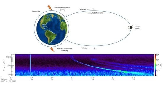
Whistler observations using spectrograms can help us understand the phenomena known as dispersion. Whistler dispersion depends on the refractive index, which is a function of the frequency, and therefore the signal propagates at different velocities at different frequencies. The propagation of whistlers along the geomagnetic field lines from the southern to northern hemispheres, and vice versa, is shown in Figure 2. The dispersion of a whistler indicates a gap in the propagation delay in the frequency domain. Lightning whistlers can propagate thousands of kilometers from the sources of the lightning strikes in the plasmasphere of the Earth, and their spectral properties primarily depend on the plasma environment (electron density and ambient magnetic field) along their propagation paths. These data are relevant to estimations of the electron density profile.

2.1. Dispersion of a Lightning Whistler

The relationship between the frequency and time of a lightning whistler is theoretically explained by Eckersley’s law [22], which proves a simple relationship between the arrival time (t) of a lightning whistler at a frequency (f) as follows:

$$t=D /\surd f+t_0$$

(2)

where D is a constant value called dispersion of lightning whistler; t is the arrival time at a frequency f; and t₀ is the time when the lightning strikes. Bayupati [15] used the simple principle of Eckersley’s law on waveform data from AKEBONO to detect lightning whistlers. The conventional technique for the automatic detection of lightning whistlers is to identify straight lines in a diagram in which the dynamic power spectra are converted into a diagram with t on the horizontal axis and 1/√f on the vertical axis. The result of this technique is shown in Figure 1, where t1 and t2 are the arrival times of the detected lightning whistler at frequencies of f1 and f2, respectively. The dispersion D of lightning whistler is determined by detecting a straight line and deriving its gradient from Equation (3).

$$D=\frac{t_2-t_1}{\frac{1}{\surd f_2}-\frac{1}{\surd f_1}}$$

(3)

It can be seen that the spectrum of lightning whistler appears as a straight line, which is well marked by thick curves as shown in Figure 1. Equations (2) and (3); however, only explain the simple relationship between frequency and time for a subset of lightning whistlers; we cannot detect other types of lightning whistlers. The other types of whistlers shown in the whistler atlas compiled by Helliwell do not satisfy this equation. Accordingly, it is necessary to develop a new method to detect various types of lightning whistlers.

2.2. Arase Whistler Map

We proposed a definition of the type of lightning whistler observed by the Arase satellite and named it the “Arase whistler map”. This whistler map is partially adapted from the original definition of the whistler atlas defined by Helliwell [17]. The principal themes of the classification definition used in Helliwell’s whistler atlas were based on ground observation result. For example, the difference between one-hop and two-hop whistler is the amount of relative dispersion, which depends on the length of propagation path. It was possible to distinguish one-hop and two-hop whistlers on ground-observations because the observation point is fixed. Such a classification is; however, not highly relevant for spacecraft observations because the observation point is always changing. Particularly for the case of very elliptical orbit such as the Arase satellite, dispersion of lightning whistler drastically changes and it is impossible to distinguish one-hop and two-hop unless the location of wave source is identified. We classified the lightning whistlers based on the duration of the whistler trace instead, because the length of duration reflects the length of propagation path from the wave source to the observation point. In addition, we classified the multiple lightning whistlers according to the combination of the durations of the traces, which suggests the existence of multiple paths.

In this paper, we develop an improved detection method, based on pattern or shape detection using image processing and image analysis approaches, via standard patterns by measuring the pixel values, line groupings, and detected line in comparison to the shapes in the reference atlas. The entire process runs concurrently, reading all the images at the same time, detecting the whistler lines, and giving the results. As we can see in

Table 1. Arase whistler map: Type and principal definitions of lightning whistlers partially adapted from the original whistler atlas by Helliwell [17].

No	Type of Whistler	Definition	Spectral Form
Single Trace
1	Nose	A whistler whose frequency-time curve exhibits both rising and falling branches. The delay is at a minimum at the nose frequency
2	Short Whistler	A whistler that has a duration of less than 1 s.
3	Middle Whisler	A whistler that has a duration between 1 s and 2 s.
4	Long Whistler	A whistler that has a duration of more than 2 s.
Multi Trace
5	Multiple-Traces	A multiple whistlers consisting of multiple basic middle whistlers with the same length of duration.
6	Multiple- Combinations	A multiple whistlers consisting of multiple basic middle whistlers with the different length of durations.

, the Arase whistler map shows the spectral forms of the lightning whistlers and distinguishes each type of whistler. We group the spectral forms into single-trace whistlers, which include nose, short, middle, and long whistlers, and multi-trace whistlers, which include the multiple-traces and multiple-combinations types. This grouping helps us formulate the classification and detection algorithm described in the next section.

2.3. Typical Shape of Lightning Whistlers Observed by Arase

There are several examples of lightning whistlers that were detected in the one-year dataset from March 2017 to March 2018 observed by WFC onboard Arase. In this section, we introduce the typical shapes of lightning whistlers observed by the Arase satellite and compare them to the Arase whistler map; nose, short, middle, long, multiple-traces, and multiple-combinations whistler measured by Arase/WFC are shown in Figure 3.

Since we did not detect the source location or the direction path of the lightning whistler, we classified the type based on only the shape or pattern representation of the lightning whistler inside the spectrogram. In the examples, as shown in Figure 3, the spectra were generated with the same period of (8 s) of data, where the X-axis indicates time and the Y-axis shows the frequency of the spectral observation. In the case of a single-trace whistler, we distinguished the type via its duration, except for the nose whistler because it has a unique shape. Meanwhile, for the case of short, middle, and long whistlers, we defined the type by its duration, as described in Table 1. In the case of multiple-traces and multiple-combinations whistlers, we checked the duration of each dispersion. When the whistler traces had the same duration, we called it a multiple-traces, whereas we called it a multiple-combinations when there were different durations. Since we only saw the whistler shape based on frequency and time points of detected whistlers, we compared the time delays of the whistlers relative to their pixel locations.

3. Flow of the Detection Process

3.1. Pre-Processing

To generate dynamic power spectra of the observed waveforms, we implemented a short-time Fourier transform analysis with a 62.5 ms Hann window that included 4096 samples with a 94% overlap (shifting the window by 256 samples). The contour unit is an arbitrary unit/Hz (dB). To obtain a better detection result, we need a clear fine structure of the dynamic spectra of a lightning whistler with a high signal-to-noise ratio. The detailed performance of the magnetic search coil magnetic sensor can be found in Ozaki et al. [21]. We applied a combination of filter operations using Gaussian filter. This technique eliminates the noisy pattern from the original spectra. To obtain the smoothing effectively, Gaussian smooth (also known as Gaussian blur) was implemented using a standard deviation sigma value of $\sigma$ = 1.

$$G_{\sigma }=\frac{1}{2\pi {\sigma }^2}exp\left\{-\frac{x^2+y^2}{2{\sigma }^2}\right\}$$

(4)

To generate a clear fine structure from the edge detector, we applied a Laplacian operation to compute the second derivative of the image resulting from the Gaussian blur. Figure 4 shows an example of the dynamic spectra of a magnetic field observed at 02:24 UT on 14 September 2017. The upper panel shows the dynamic spectra processed from the WFC data, and the lower panel shows the edge spectra after using Gaussian blur and Laplacian filtering to remove noise. As can be seen in the upper panel, the clear fine structure of the lightning whistler is characterized by a discrete tone that decreases in frequency with increasing time. The bottom panel shows the clear result of a whistler trace in the dynamic spectra after implementing the Gaussian blur and edge detection via the Laplacian filter. We then performed the above-mentioned pre-processing on the result of the dynamic power spectra and saved it to an image file (PNG format) that fit our monitor size resolution of 1920 × 1017 pixels. The saved file has the same information as shown in Figure 4. This file was then used as input for our detection system. The total number of spectral image data files produced during the observations is shown in

Table 2. Total numbers of the spectra image file as a function of month.

Year	2017										2018
Month	Mar	Apr	May	Jun	Jul	Aug	Sep	Oct	Nov	Dec	Jan	Feb	Mar
Total Files	2102	649	2088	3209	2319	2205	5027	3378	3021	1696	2153	2163	1370

.

3.2. Overview of the Detection System

Figure 5 shows the overall flow chart of our proposed whistler detection method. The quality of the input image of the candidate area directly affects the accuracy of the target detection task. We have two different spectra (original and pre-processed), as shown in Figure 4. To extract information from the input image, our detection system only uses the segmented input image from the pre-processed spectra. This operation not only accelerates the speed of target detection but also improves the detection performance, because the information has a clear fine structure with the unwanted information eliminated (e.g., the attached noise).

The segmentation target area indicates an area with an important detection where a lightning whistler is located. We define a partitioned area inside this area, then split it into grid lines, as shown in Figure 6. Each grid line represents information about the time and frequency. The X-axis represents the time of the observation with 100-ms increments. The Y-axis represents the frequency on a logarithmic scale. Then, we calculate the average of each pixel point for every represented grid point. We limited the detection frequency range from 1 kHz to 20 kHz. The segmentation result of the image grid of the target area was produced using the OpenCV function and the neighboring pixel relation (N8). Groups of pixels of the binary image with similar features (colors) are obtained, in which the whistler region is 1 (non-white) and the non-whistler region is 0 (white). Subsequently, we used Bresenham’s line algorithm [23] for every step after segmentation, from line grouping, line detector, and line counter. Bresenham’s algorithm is a widely used high-speed algorithm that rasterizes straight lines/circles/ellipses using only addition and subtraction operations of pure integers; description and the concept of this algorithm is available in Reference [23].

The process of line grouping starts from a neighboring pixel that is connected with the Bresenham function; then the pixels are grouped as a line-group. Further, the area of the adjacent neighboring block is scanned with triangular scanning to locate the boundary. The checked block is eliminated and then another block is moved to that is already marked as a line-group. After the line-group is connected, we add labeling for each starting and ending point of the line-group associated with the pixel position of the grid corresponding to time on the X-axis and frequency on the Y-axis. Examples of detected lines are shown in Figure 7. Then, the detected lines are analyzed one by one as whistler traces: Single lines that represent a whistler. There are two types of whistler traces: Single traces and multi-traces. The system marks each starting and ending point (x, y) of the whistler trace, compares its location based on the pixel grid, and stores the corresponding information. The X-axis (time) indicates the duration of the lightning whistler, and the Y-axis indicates its frequency.

According to the Arase whistler map, there is one type of whistler that is distinguished by a different shape than the others, the nose whistler. The others have the shape of a normal whistler and are either single-trace or multi-trace whistlers. The duration of lightning whistlers as well as their combination is important when deciding the type of lightning whistler propagating in geospace.

We developed a classification rule and principle, in which the nose whistler is checked for before the other types are detected. The detection process starts with line-group counting. If no line-group exists, the event is identified as no-whistler. If a line-group exists, the next step is to determine if it complies with the nose whistler check criteria. If yes, then we mark it as a nose whistler. If we fail to detect a nose shape, then we check the number of line traces in the line-group process, we categorize it as a single-trace or multi-trace whistler, and then we check the duration of each trace line detected. The event will then be classified based on the rules that can be summarized as shown in Figure 8.

To successfully detect a nose whistler, we define a criteria-matching region as shown in Figure 9. The explanation of this region is as follows. The black line is an example of a nose whistler existing in a diagram of the dynamic spectra. It has a starting point, which is marked as XsYs and an ending point marked XeYe. As a reference of the Cartesian axis, the orange line represents the Y-axis (frequency) and the purple line represents the X-axis (time). The green region is located to the left of the Y-axis, and the blue region is located to the right of the Y-axis. These two regions will help us determine whether the component of the targeted whistler trace/whistler line belongs to the criteria matching a nose whistler.

We developed an algorithm to check for nose whistlers first; this algorithm is the first step before we can successfully detect all other types of lightning whistler. The pseudo code and detailed detection of a nose whistler are described in Algorithm 1.

Algorithm 1 The Nose-whistler detection algorithm

1 For each line-group in the image

2 Find the maximum frequency and time on the X-axis and Y-axis (XsYs)

3 var Ys = line_group.Min(s => s.point.Y);

4 var Xs = line_group.Where(s => s.point.Y == Ys).Min(s => s.point.X);

5 Find the lowest time point on the X-axis

6 var left_x = line_group.Min(s => s.point.X);

7 Find the lowest frequency point on the Y-axis

8 var left_y = line_group.Where(s => s.point.X == left_x).Max(s => s.point.Y);

9 Compare the pixel location region of the starting time

10 if (left_x >=Xs)

11 return false;

12 Compare the pixel location region of the whistler trace in the green region

13 if ((left_x <= Xs - (1 * line_group.neighborInterval) && left_y - Ys >

14 line_group.neighborInterval + 1) == false)

15 return false;

16 Find the lowest frequency point of the start point of the whistler trace on the Y-axis

17 var bottom_y = line_group.Max(s => s.point.Y);

18 Find the lowest frequency point of the last point of the whistler trace on the Y-axis

19 var bottom_x_fr_bottom_y = line_group.Where(s => s.point.Y == bottom_y).Max(s => s.point.X);

20 Compare the pixel location region of the whistler trace in the blue region

21 if (bottom_x_fr_bottom_y >= Xs + (1 * line_group.neighborInterval)) == false)

22 return false;

23 Detection result

24 whistler.type = WhistlerModelType.Nose;

25 return true;

4. Experimental Result and Discussion

To evaluate the performance of the proposed method, we tested a set of real images of dynamic spectra produced by WFC. The entire experiment was performed on a Core-i7-4810 MQ 2.8 GHz (8 CPUs) with 16 GB of RAM. Before processing the entire dataset, we tested the detection algorithm for each type of lightning whistler, as can be seen in Figure 10 and Figure 11. The detected whistler is traced by a box, and the result of each detection is stored in a text file with each characteristic, including type, start time, end time, start frequency, end frequency, and time consumed for each detection process. Some whistlers were not detected due to the density between pixels. We rely on the concept of the neighboring pixel, so if the filtering in the pre-processing results in a weakly connected or un-connected line, this will affect our detection system. The event will not be detected as a line because it is not a single connected line. To prevent this and improve the detection accuracy, it is necessary to develop an intermediate process between spectral filtering and detection. This process should make adjustments to maintain the pixel quality, prevent pixel loss, and refine connected lines to improve the detection process and increase the accuracy.

For comparison with the algorithm result, we used “manual inspection” that we made a year before we developed this application, that is, we conducted a direct inspection to identify all the available image spectra. In this observation, we visually inspected, one by one, every image spectra and investigated the detected lightning whistlers via the spectrogram. Since this type of observation depends solely on the experience of the investigator, the manual inspection took a long time and we checked every detail of each spectrogram and carefully marked the event and type using the principles defined in the Arase whistler map. In our detection policy for automatic detection, we prioritize highest accuracy of false-detection. False-detection means that shape of lightning whistler trace is inappropriately detected and thus differently classified because of the background noise. To decrease the false-detection rate, a higher threshold level is necessary, but it causes an increase in mis-detection rate. Here mis-detection means that weak lightning whistler cannot be detected due to faint and patchy line that fails line grouping by the Bresenham’s line algorithm. Using optimized parameters, we performed bulk processing of detection for one-year data. To use our proposed algorithm, we loaded all the images as input into the application, and the application processed each detection concurrently with the available CPU and memory. It took 30 h to completely detect all the whistlers in the available dataset. Some whistlers were not detected due to our detection policy. The result of the detection system as output from the application is shown in

Table 3. The comparison detection result using the defined algorithm and manual inspections.

Automatic Lightning Whistler Detection: Output Result
Total number of 1-Year observation image spectra	31,380 image file
Spectra with whistler event from manual inspection	949 image file
Spectra with whistler event from automatic detection	711 image file
Mis-detection rate	25.07%
Detection configuration: frequency threshold	1 kHz to 20 kHz
Number of line-group detected	1165
Number of detected whistler	Whistler type: single-trace				Whistler type: multi-traces
	Nose	Short	Middle	Long	Multiple-traces	Multiple-combinations
	58	147	238	-	340	382

. There are 711 image files in which we could detect lightning whistlers, while 1165 of line groups were identified among the 711 image files. We couldn’t detect any long whistlers when we apply the optimized parameter. In fact, we can detect a long whistler as shown in Figure 10, if we optimize the parameter only for this event, but it causes an increase of false detection rate for the other events due to contaminated noise. In future work, we need to solve this problem of how to reduce the noise or add some denoising technique in order to get better pre-processed spectra.

We assume that the manual inspections are more reliable than the automatic detection because the algorithm still has a limited capability and further work needs to be done to improve it, such as selecting different types of filtering to improve the quality of the input image in the pre-processing and to increase the detection accuracy. By detecting whistler using duration approached, our classification system has decreased the number of false classifications. False classification mean that the system classified the wrong type of lightning whistler within the same criteria. It most likely happens when the false line detected as lightning whistler. In Table 3, we show that we could not classify the long whistler. Actually, we observed the long whistler in manual inspection, but all events to be categorized into long-whistler were mis-detected due to our amplitude threshold level.

5. Conclusions

In this paper, we presented the detection methodology for various types of lightning whistlers observed by WFC onboard the Arase satellite. The lightning whistler data were captured by the WFC magnetic field component during a one-year observation period from March 2017 to March 2018. Each footprint of the magnetic field during the observation period was converted into dynamic spectra and stored in an image file. We collected the image files and developed a detection system for the lightning whistlers captured inside the images. Using image processing and image analysis approaches, we developed a methodology and classification system to automatically detect lightning whistlers that is robust, fast, and informative. The detection results were very accurate, and six types of lightning whistler were successfully classified. The various types of lightning whistler detected by WFC onboard the Arase satellite will correspond to study of propagation characteristic of the signal of whistler waves depending on the region.

References

1. Eckersley, T.L. Musical Atmospherics. Nature 1935, 135, 104–105. [Google Scholar] [CrossRef]
2. Storey, L.R.O. An investigation of whistling atmospherics. Phil. Trans. Roy. Soc. 1953, 246, 113–141. [Google Scholar] [CrossRef]
3. Carpenter, D.L. Whistler evidence of a ‘knee’ in the magnetospheric ionization density profile. J. Geophys. Res. 1963, 68, 1675–1682. [Google Scholar] [CrossRef]
4. Abel, B.; Thorne, R.M. Electron scattering loss in Earth’s inner magnetosphere: 1. Dominant physical processes. J. Geophys. Res. 1998, 103, 2385–2396. [Google Scholar] [CrossRef]
5. Rostoker, G.; Skone, S.; Baker, D.N. On the origin of relativistic electons in the magnetosphere associated with some geomagnetic storms. Geophys. Res. Lett. 1998, 25, 3701. [Google Scholar] [CrossRef]
6. Elkington, S.R.; Hudson, M.K.; Chan, A.A. Acceleration of relativistic electrons via drift-resonant interaction with toroidal-mode Pc-5 ULF oscillations. Geophys. Res. Lett. 1999, 26, 3273. [Google Scholar] [CrossRef]
7. Lauben, D.S.; Inan, U.S.; Bell, T.F. Precipitation of radiation belt electrons induced by obliquely propagating lightning-generated whistlers. J. Geophys. Res. 2001, 106, 29745–29770. [Google Scholar] [CrossRef]
8. Rodger, C.J.; McCormick, R.J.; Clilverd, M.A. Testing the importance of precipitation loss mechanisms in the inner radiation belt. Geophys. Res. Lett. 2004, 31, L10803. [Google Scholar] [CrossRef]
9. Millan, R.; Thorne, R. Review of radiation belt relativistic electron losses. J. Atmos. Sol. Terr. Phys. 2007, 69, 362–377. [Google Scholar] [CrossRef]
10. Meredith, N.P.; Horne, R.B.; Glauert, S.A.; Baker, D.N.; Kanekal, S.G.; Albert, J.M. Relativistic electron loss timescales in the slot region. J. Geophys. Res. 2009, 114, A03222. [Google Scholar] [CrossRef]
11. Santolík, O.; Parrot, M.; Inan, U.; Burešová, D.; Gurnett, D.; Chum, J. Propagation of unducted whistlers from their source lightning: A case study. J. Geophys. Res. 2009, 114, A03212. [Google Scholar] [CrossRef]
12. Fiser, J.; Chum, J.; Diendorfer, G.; Parrot, M.; Santolik, O. Whistler intensities above thunderstorms. Ann. Geophys. 2010, 28, 37–46. [Google Scholar] [CrossRef] [Green Version]
13. Zheng, H.; Holzworth, R.H.; Brundell, J.B.; Jacobson, A.R.; Wygant, J.R.; Hospodarsky, G.B.; Mozer, F.S.; Bonnell, J. A statistical study of whistler waves observed by Van Allen Probes (RBSP) and lightning detected by WWLLN. J. Geophys. Res. Space Phys. 2016, 121, 2067–2079. [Google Scholar] [CrossRef]
14. Záhlava, J.; Němec, F.; Santolík, O.; Kolmašová, I.; Hospodarsky, G.B.; Parrot, M.; Kurth, W.S.; Bortnik, J.; Kletzing, C. Longitudinal dependence of whistler mode electromagnetic waves in the Earth’s inner magnetosphere. J. Geophys. Res. Space Phys. 2018, 123, 6562–6575. [Google Scholar] [CrossRef]
15. Bayupati, I.P.A.; Kasahara, Y.; Goto, Y. Study of Dispersion of Lightning Whistler observed by Akebono Satellite in the Earth’s Plasmasphere. IEICE Trans. Commun. 2012, E95-B, 3472–3479. [Google Scholar] [CrossRef]
16. Oike, Y.; Kasahara, Y.; Goto, Y. Spatial distribution and temporal variations of occurrence frequency of lightning whistlers observed by VLF/WBA onboard Akebono. Radio Sci. 2014, 49, 753–764. [Google Scholar] [CrossRef]
17. Helliwell, R.A. Whistlers and Related Ionospheric Phenomena; Stanford Univ. Press: Stanford, CA, USA, 1965. [Google Scholar]
18. Miyoshi, Y.; Shinohara, I.; Takashima, T.; Asamura, K.; Higashio, N.; Mitani, T.; Kasahara, S.; Yokota, S.; Kazama, Y.; Wang, S.Y.; et al. Geospace exploration project ERG. Earth Planets Space 2018, 70, 101. [Google Scholar] [CrossRef] [Green Version]
19. Kasahara, Y.; Kasaba, Y.; Kojima, H.; Yagitani, S.; Ishisaka, K.; Kumamoto, A.; Tsuchiya, F.; Ozaki, M.; Matsuda, S.; Imachi, T.; et al. The plasma wave experiment (PWE) on board the Arase (ERG) satellite. Earth Planets Space 2018, 70, 86. [Google Scholar] [CrossRef]
20. Matsuda, S.; Kasahara, Y.; Kojima, H.; Kasaba, Y.; Yagitani, S.; Ozaki, M.; Imachi, T.; Ishisaka, K.; Kumamoto, A.; Tsuchiya, F.; et al. Onboard software of plasma wave experiment aboard Arase: Instrument management and signal processing of waveform capture/onboard frequency analyzer. Earth Planets Space 2018, 70, 75. [Google Scholar] [CrossRef]
21. Ozaki, M.; Yagitani, S.; Kasahara, Y.; Kojima, H.; Kasaba, Y.; Kumamoto, A.; Tsuchiya, F.; Matsuda, S.; Matsuoka, A.; Sasaki, T.; et al. Magnetic search coil (MSC) of plasma wave experiment (PWE) aboard the Arase (ERG) satellite. Earth Planets Space 2018, 70, 76. [Google Scholar] [CrossRef]
22. Gurnett, D.A.; Kurth, W.S.; Cairns, I.H.; Granroth, L.J. Whistler in Neptune’s Magnetosphere: Evidence of Atmospheric Lightning. J. Geophys. Res. 1990, 95, 20967–20976. [Google Scholar] [CrossRef]
23. Bresenham, J.E. A linear algorithm for incremental digital display of circular arcs. Commun. ACM 1977, 20, 100–106. [Google Scholar] [CrossRef]
Figure 1. An example of a frequency–time spectrum of a lightning whistler observed on 21 June 1997, from AKEBONO, with the marked lightning whistler detected using the 1/√f conversion technique (image source [15]).
Remotesensing 11 01785 g001
Figure 2. Propagation path of a lightning whistler.
Remotesensing 11 01785 g002
Figure 3. (a) Nose whistler at 10:44:27 UT on 27 September 2017; (b) short whistler at 14:24:08 UT on 2 October 2017; (c) middle whistler at 02:24:18 UT on 14 September 2017; (d) long whistler at 02:26:22 UT on November 18, 2017; (e) multiple-traces at 08:39:45 UT on 7 September 2017; (f) multiple-combinations at 16:37:18 UT on 9 October 2017, observed by the PWE/WFC (plasma wave experiment/waveform capture).
Remotesensing 11 01785 g003
Figure 4. (top) The original middle whistler dynamic spectra observed at 02:24:17 UT on September 14, 2017. (bottom) Edge spectra after using a Gaussian blur with a mask (1,0.1) and Laplacian filtering to remove noise.
Remotesensing 11 01785 g004
Figure 5. The overall flow chart of the whistler detection system. The process from left to right shows segmentation, extraction of the candidate area, the classification rule, and the detection result.
Remotesensing 11 01785 g005
Figure 6. The segmentation of an input image of a 4-s duration observation into a grid line to extract the corresponding information.
Remotesensing 11 01785 g006
Figure 7. The result of the detected line and grouped as line-group.
Remotesensing 11 01785 g007
Figure 8. Decision tree for the all-whistler classifier.
Remotesensing 11 01785 g008
Figure 9. Nose-whistler detection criteria-matching region.
Remotesensing 11 01785 g009
Figure 10. The detected nose, short, middle, and long whistler types.
Remotesensing 11 01785 g010
Figure 11. The detected multiple-traces and multiple-combinations whistler types.
Remotesensing 11 01785 g011