Urban Flood Detection with Sentinel-1 Multi-Temporal Synthetic Aperture Radar (SAR) Observations in a Bayesian Framework: A Case Study for Hurricane Matthew

Abstract

In this study we explored the application of synthetic aperture radar (SAR) intensity time series for urban flood detection. Our test case was the flood in Lumberton, North Carolina, USA, caused by the landfall of Hurricane Matthew on 8 October 2016, for which airborne imagery—taken on the same day as the SAR overpass—is available for validation of our technique. To map the flood, we first carried out normalization of the SAR intensity observations, based on the statistics from the time series, and then construct a Bayesian probability function for intensity decrease (due to specular reflection of the signal) and intensity increase (due to double bounce) cases separately. We then formed a flood probability map, which we used to create our preferred flood extent map using a global cutoff probability of 0.5. Our flood map in the urban area showed a complicated mosaicking pattern of pixels showing SAR intensity decrease, pixels showing intensity increase, and pixels without significant intensity changes. Our approach shows improved performance when compared with global thresholding on log intensity ratios, as the time series-based normalization has accounted for a certain level of spatial variation by considering the different history for each pixel. This resulted in improved performance for urban and vegetated regions. We identified smooth surfaces, like asphalt roads, and SAR shadows as the major sources of underprediction, and aquatic plants and soil moisture changes were the major sources of overprediction.

1. Introduction

Flood extent maps based on synthetic aperture radar (SAR) have increasingly been used in recent emergency response operations. For example, in the Sentinel Asia consortium (https://sentinel.tksc.jaxa.jp), where national space agencies, research institutions, and end-user organizations work together on emergency observation requests in the Asia-Pacific region, the responses to 20 of 23 activated flood-related events in the year of 2017 used ALOS-2 SAR flood-mapping results [1]. These statistics demonstrate the need for radar’s all-weather, day-and-night sensing capability, where in most cases cloud cover and rains persist for the duration of a flood.

Flood extent maps are primarily extracted from SAR intensity (the squared amplitude of the SAR return) information. The backscattering coefficient (σ⁰, log intensity in dB) decreases due to the specular surface of open flood waters if radar energy is mostly forward-scattered. In other cases, σ⁰ may increase if the radar wave bounces first off the water surface (away from the satellite) and then off a semivertical structure, such as a building wall, tree trunk, or even a car in the flood (towards the satellite); this is the “double bounce” effect. Compared with rural floods, urban flood mapping suffers more from layover and shadow effects due to SAR’s side-looking nature. The layover zone is in front of buildings, toward the satellite direction, and the length is usually longer than the building height at incidence angles lower than 45° (layover length = building height × cot(incidence angle) [2]). Within this zone there is a good chance of seeing stronger backscattering due to the double bounce effect, and its strength is a function of the oblique angle between the flight direction and the building orientation. The double-bounce intensity increase can be larger than 10 dB at 0° and remains high up to 5°; at an angle larger than 10° the increase will drop to a constant level [3,4]. The shadow zone, on the other hand, has a smaller length (shadow length = building height × tan(incidence angle) [2]), and the backscattering stays low at all times. The low intensity within the shadow may lead to false flood detection if one uses a during-flood SAR image alone.

Several studies have tried to improve the accuracy of urban flood mapping by addressing layover and shadow effects. For example, Mason et al. and Giustarini et al. [2,5,6], for a case study using TerraSAR-X data, masked out the layover and shadow zones by using a SAR simulator. The accuracy of open water flood mapping increases after applying the mask, but flooded pixels that show increased brightness due to double-bounce scattering are left out from the flood map. In another example, Pulvirenti et al. [7] developed an algorithm that adopted the double-bounce intensity values from electromagnetic modeling as initial fuzzy thresholds, and they used fuzzy logic to map out the urban flood with intensity increase in COSMO-SkyMed images. Mason et al. [8] also demonstrated the use of an electromagnetic scattering model and high-resolution elevation data to simulate the double-bounce effects. The simulated double-bounce scattering strength agrees with the observed data; hence, it can provide information about the statistical distribution of pixels showing double bounce for better thresholding decisions. Both model-based approaches have the advantage of being independent from user biases when handling double-bounce effects, although the auxiliary data of a high-resolution building model (or digital surface model) is not always available. Tanguy et al. [9] proposed to use ancillary hydraulic data to refine the flood detected with RADARSAT-2 so as to overcome the SAR limitations associated with viewing geometry. The availability of such high-resolution hydraulic data is not, however, guaranteed. Recently, some studies have found that using interferometric coherence in conjunction with intensity will improve the detection accuracy particularly associated with double bounce [4,10,11,12]. The efficacy of augmenting moderate resolution interferometric coherence (from Sentinel-1 SAR, for example) in urban flood detection still awaits systematic, quantitative validation [10].

In parallel to the developments in urban flood mapping, multitemporal SAR data analyses are also gradually being adopted by scientists to study flood extents. Hostache et al. [13] suggested to select the most appropriate pre-flood image for change detection from a time series perspective. Schlaffer et al. [14,15] carried out harmonic analysis on seven years of ENVISAT ASAR data and identified floods by looking at anomalies in the time series. D’Addabbo et al. [16] utilized Bayesian networks to jointly consider SAR intensity and InSAR coherence time series of COSMO-SkyMed data, as well as ancillary information including several hydraulic parameters, to study flood extent variation over time. Clement et al. [17] utilized Sentinel-1 SAR intensity difference (change detection) time series to identify the evolution of a flood with time. Ouled Sghaier et al. [18] utilized texture analysis on multitemporal RADARSAT-2 and Sentinel-1 intensity data to study flood history. Among these studies, some of them focus on flood evolution and treat each epoch independently, while others emphasize the use of pixel history to improve the accuracy of flood detection on particular events.

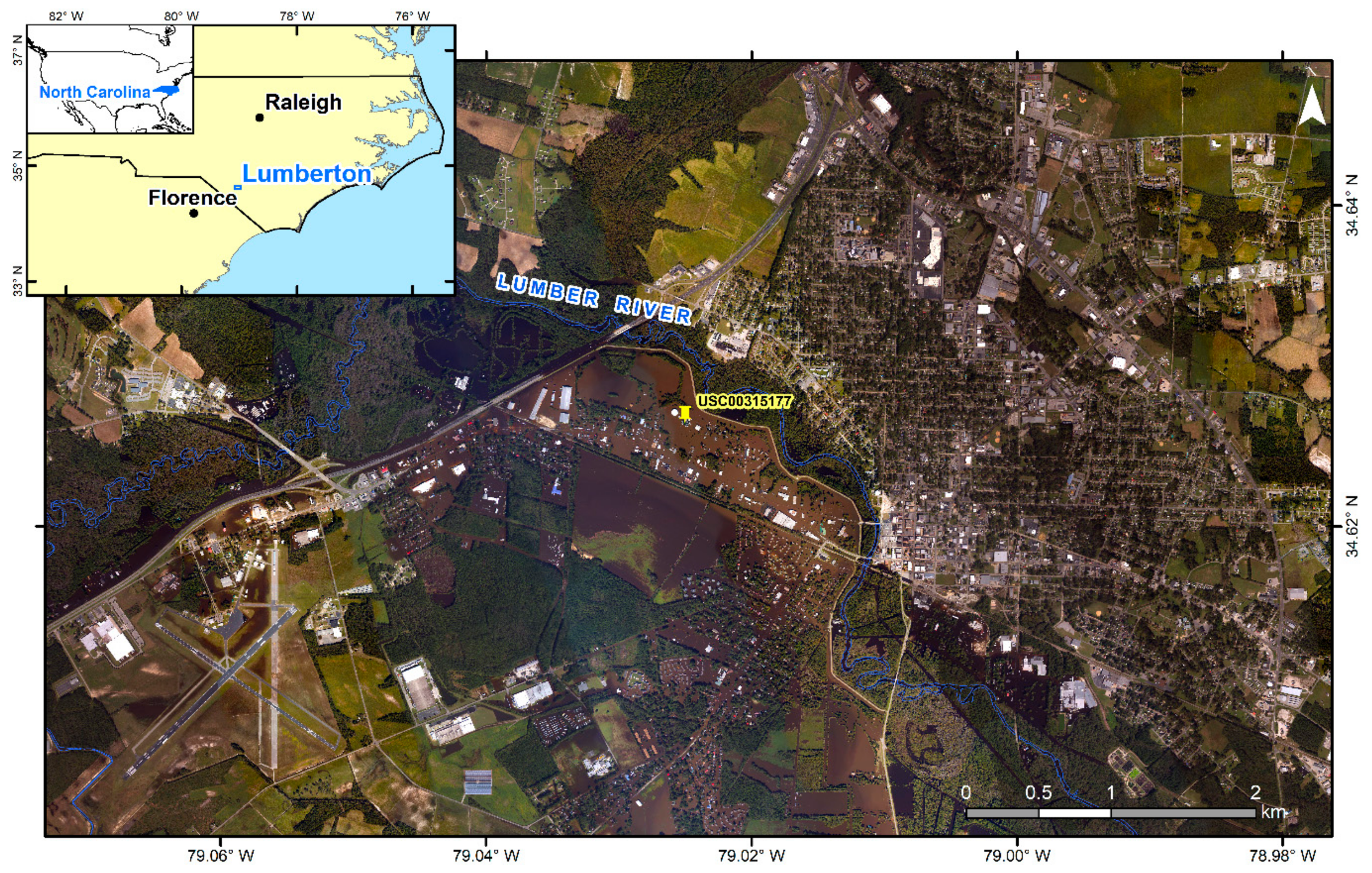
The approach that we propose in this study focuses on both the urban and time series dimensions. We would like to obtain the statistics of each pixel from the time domain and use them in a Bayesian flood probability function. The flood probability is calculated based on the historical pixel intensity values. The test data are Sentinel-1 SAR, whose open access and short repeat time make them a priority choice in many emergency response cases. We test our approach on the Hurricane Matthew flood in early October 2016 at the town of Lumberton, in North Carolina, USA. The Lumberton flood offers a great opportunity in which nearly concurrent airborne optical imagery and spaceborne SAR observations coexist for the flooding epoch. It is also an ideal target to examine the efficacy of urban flood mapping algorithms, as more than half of the flooded areas are in urban settings.

2. Study Area and Data

2.1. Study Area and Weather Event

Lumberton is located on the Coastal Plains of North Carolina, with an average elevation of 40 m and the Lumber River flowing through the town center (Figure 1). The test area was right around the town center, approximately 5.5 × 12 km in dimension, with ~30% of the area being an urban environment.

On 8 October 2016, Hurricane Matthew made landfall on the southeast coast of South Carolina and slowly moved northwards into North Carolina. Even though it had significantly weakened from a Category 5 to Category 1 hurricane at the time of landing, and was an extratropical cyclone by the time it arrived at North Carolina [19], torrential rains still brought >200 mm cumulative precipitation depths on 9 October (according to the National Oceanic and Atmospheric Administration (NOAA)’s ground weather station USC00315177; see Figure 1 for location) and caused record-breaking flood levels along the Lumber River. A levee broke, resulting in four flood-related deaths and more than 1500 people evacuated. Most of the region was still in knee-deep water two days after the hurricane passed [19].

2.2. Optical and Synthetic Aperture Radar (SAR) Imagery

Because the Carolinas experienced such serious flooding during the hurricane, the National Oceanic and Atmospheric Administration (NOAA) Remote Sensing Division acquired inland aerial photos between 11–16 October as rapid response imagery using a nadir-looking camera mounted on NOAA’s King Air 350ER aircraft [20]. The Lumberton swath was taken during the daytime (around noon local time, from 15:53 to 16:35 UTC) on 11 October at a ground resolution of ~30 cm (Figure 1). The same-day Sentinel-1A interferometric wide swath SAR image was acquired at 19:13 EDT (23:13 UTC). Given the seven-hour difference in the acquisition time, there will be some small but minimal differences between the flood extents mapped from the two datasets, with potentially smaller flood areas recorded in the SAR image.

Besides the aerial photos taken by NOAA, we also obtained a SPOT-6 image acquired on 6 September 2016 in order to study the pre-flood water bodies. This image, together with other historical WorldView/QuickBird images available on Google Earth, showed that the location and area of pre-existing water bodies along the Lumber River remained fairly constant through time.

For the SAR imagery, we obtained all scenes available in ascending track 77 that covered Lumberton since the beginning of the Sentinel-1 mission until the end of August 2018. There is a total of 63 images, including the during-flood scene on 11 October 2016. Descending track 84 that covers this region only contains 2 images throughout the whole time; therefore, we excluded the descending track from our analysis. We treated all scenes except for the 11 October scene as nonflood imagery in our multitemporal analysis, assuming a stationarity in land cover for all times except when the flood occurred. All SAR images were processed and geocoded at 15 × 15 m ground pixel spacing using a SRTMv3 DEM [21] oversampled by a factor of two.

3. Data Processing and Analysis

3.1. Validation Dataset

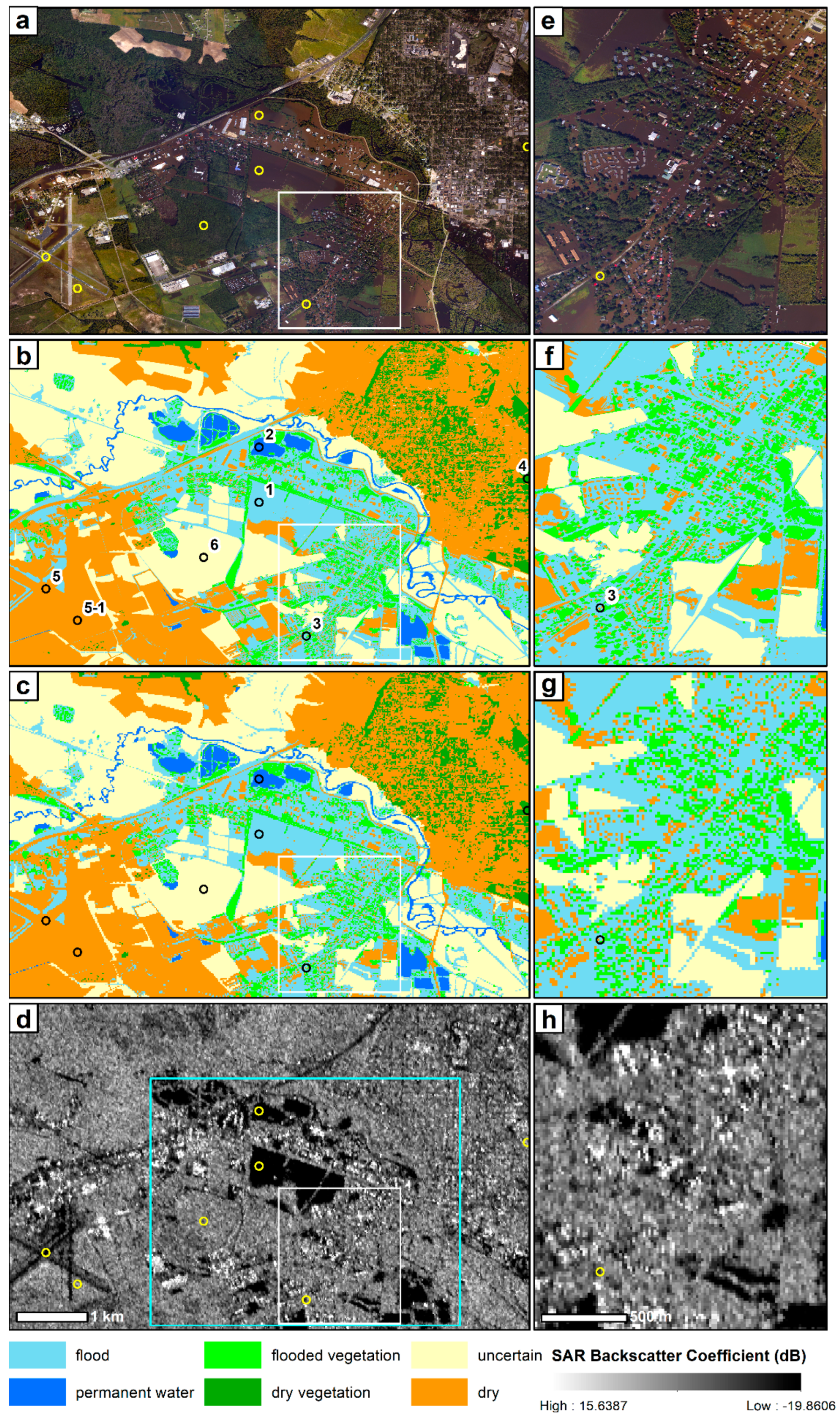
Radar intensity data contain more complicated responses than a simple binary dissection between wet and dry areas. We therefore decided to create a validation dataset that also honored possible SAR σ⁰ responses based on different land cover types. We manually classified the during-flood aerial image into the following six classes (

Table 1. Classes in the validation dataset and their backscattering responses.

	Responses in During-Event Scene
	Intensity Drop	Intensity Increase	Intensity Stays Low	Intensity Stays High
Flooded	Flood	Flood
		Flooded Vegetation
Nonflooded			Permanent Water	Dry Vegetation
			Dry	Dry
Not Determined	Uncertain (not considered in evaluation metric)

and Figure 2):

Flood: This class was the open standing water surface as directly seen in the aerial image. It was considered as an area of flooding associated with Hurricane Matthew. Intensity may decrease or increase in the during-event epoch depending on the incidence angle of the SAR image and the proximity of the pixel to any nearby vertical structures, such as trees or buildings.

Permanent Water: This class was identified based on the water bodies in the pre-flood SPOT-6 image. The SAR σ⁰ tended to stay low both in the non- and during-event images given the constant specular reflection surface at all times.

Flooded Vegetation: This class represented small to medium-size patches of trees surrounded by flood water from Hurricane Matthew. They mainly appeared in the urban area of Lumberton. Whether the radar wave penetrated the tree crowns was subject to factors like radar wavelength, polarization, and the density and structure of vegetation. If it did, double bounce and enhanced backward scattering may occur, resulting in an increase in the during-event σ⁰. If the tree crown was too dense to penetrate, SAR σ⁰ stayed relatively stable with potential seasonal variations.

Dry Vegetation: This class stood for small to medium-size patches of trees standing on dry land. The SAR σ⁰ should also stay at a relatively constant level with potential seasonal variations.

Dry: The dry class represented buildings, roads, dry bare land or lawns. Any pixels that appeared to be dry without ambiguity of underlying flood water were included in this class. The pixel values may vary with time depending on the detailed land cover type (paved road, lawn, bare soil, etc.). We did not expect to see significant intensity anomalies in buildings and roads on the during-event epoch, although intensity changes associated with soil moisture may be observed on the bare land or lawns.

Uncertain: A large area of the Lumberton region is covered by dense forest where the Lumber River flows through. Careful investigation of the spatial context showed that many of these large forest patches were surrounded by flood water on all sides. What remains unclear is whether if there was also flood water under the tree canopy. To honor this unidentifiable condition based on the high-resolution optical imagery, we classified these large forest patches as uncertain. The SAR σ⁰ may stay at a relatively high level due to the dense tree tops, but the actual level and the during-event response may vary within the same forest patch. We did not include pixels in this class in the final confusion matrix calculation.

After manual classification was done, we applied a nearest-neighbor sampling to convert the validation vector data of 30 cm resolution (Figure 2b) into a raster image of 15 m resolution (Figure 2c). We took cautious steps to ensure that each pixel in the converted raster image registered to the pixels in the SAR image. Note that there was potential change or loss of information during the down-sampling. We also tested converting the vector file into a 30 m raster image, and the result showed significant loss of spatial context, especially in urban regions. For example, buildings were concatenated together or coalesced with trees; and smaller buildings could fully disappear. Our conclusion is that 15 m ground resolution is minimally needed to undertake proper flood mapping in urban regions.

3.2. Sentinel-1 SAR Data Processing

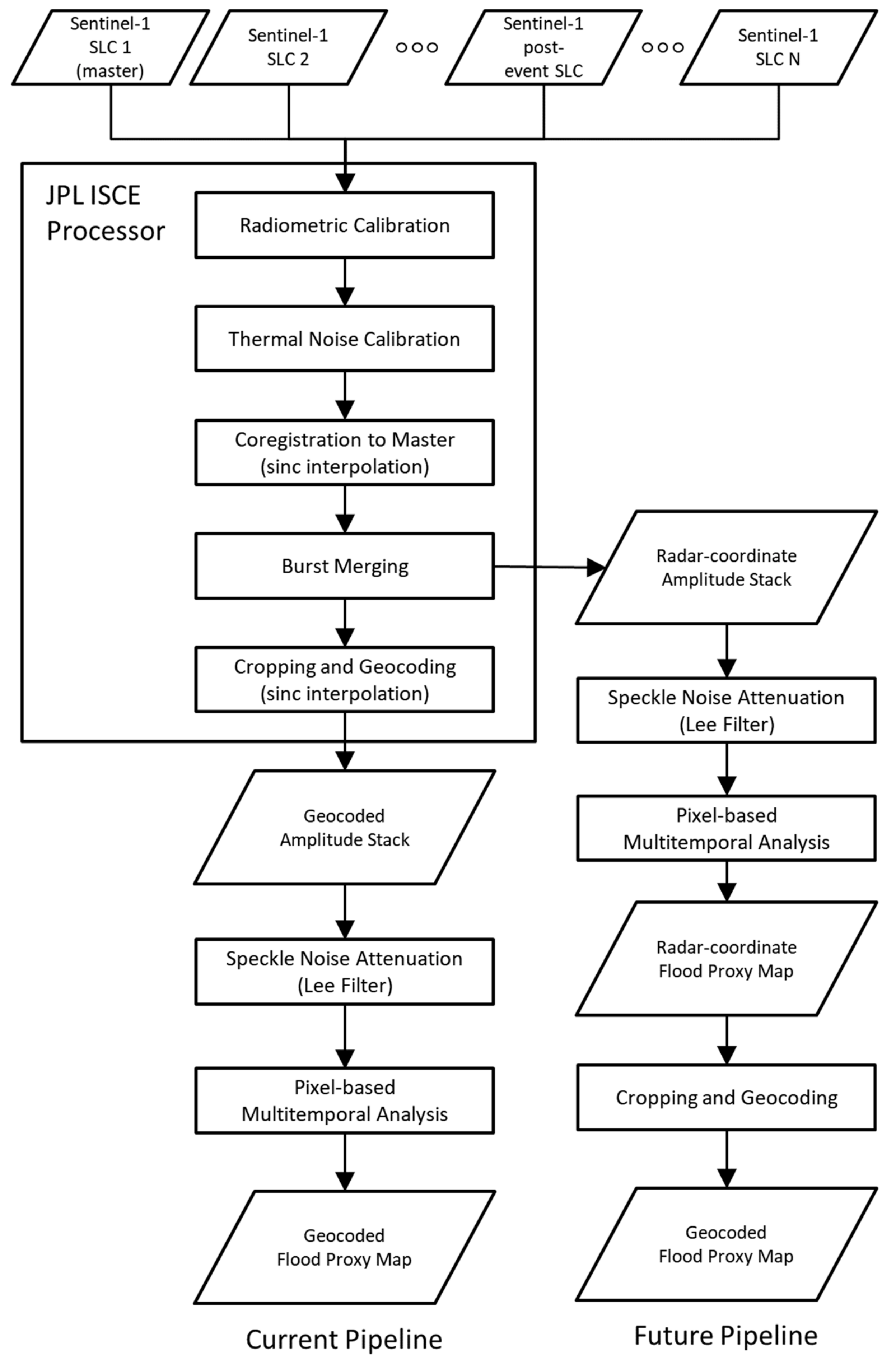
We developed our amplitude stack processing pipeline using the NASA Jet Propulsion Laboratory’s InSAR Scientific Computing Environment (ISCE) version 2 (ISCE2 is now open-sourced at GitHub: https://github.com/isce-framework/isce2). In this pipeline (Figure 3), we started from SLC files in VV polarization mode, and incorporated Sentinel-1 radiometric calibration and thermal noise calibration [22] on a burst-by-burst basis. Then we co-registered all slave images to a single master image before merging the bursts. In this study, to ensure proper comparison with the validation dataset, we produced a stack of intensity images in georeferenced coordinates. For an actual operational system, we would switch to stack processing in radar coordinates.

After producing the geocoded amplitude stack of 15 × 15 m posting, we applied a 5 × 5 Lee filter [23,24] to reduce speckle noise. We also tested 3 × 3 and 7 × 7 Lee filters, and comparison with the validation dataset shows that the 5 × 5 window gave the optimal result at a ground pixel spacing of 15 × 15 m. Since the incidence angle variation was small across the study area, from 35.7° at near range to 36.4°at far range, and the Lumberton region is relatively flat, we skipped the local incidence angle correction proposed by [25]. Finally, we computed the backscattering coefficients (σ⁰) in decibels (dB) by the following definition:

$${\sigma }^0=10lo{g}_{10}\left(A^2\right)$$

(1)

where A stands for the amplitude of the SAR image in the complex domain after radiometric calibration and thermal noise calibration [22]. We then looked into these σ⁰ values on a pixel-by-pixel basis in the following multitemporal analysis.

3.3. SAR Intensity Time Series

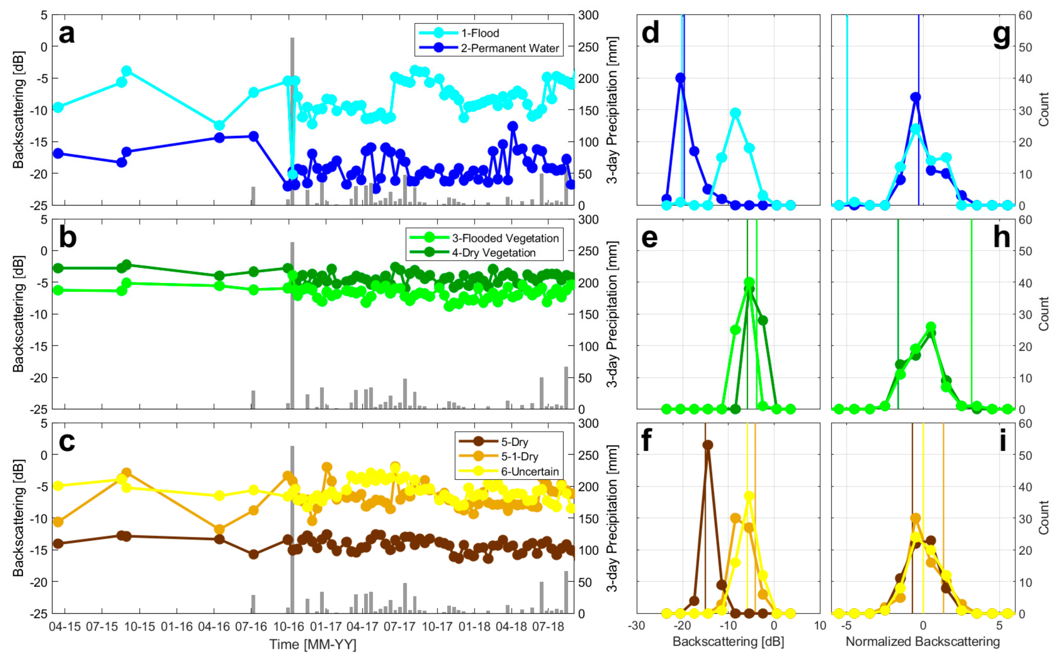
We first tried to observe if there was any characteristic temporal pattern associated with each of the six classes defined in Section 3.1. For the Flood class (Figure 4a), we picked a pixel sitting in the middle of open standing water (sample pixel 1 in Figure 2), and we observed a significant intensity decrease (~15 dB) for the during-event epoch, while the background value remained between −5 and −12 dB. It is worth pointing out that the histogram for this pixel (Figure 4b) looked similar to the Dry class (Figure 4f), reflecting the nature that this pixel was dry under ordinary conditions. The flood epoch was, therefore, an outlier (vertical line in Figure 4b) from the dry epochs, and this formed the core of our flood detection approach (Section 4).

We picked the sample pixel for the Permanent Water class in the middle of a pond. Its σ⁰ slightly varied with time but mostly stayed low, around −20 dB (Figure 4a; sample pixel 2 in Figure 2). In some epochs the value may go 5 dB higher, close to some of the nonflooded epochs in the flood class. This natural variation may be associated with the changes of floating aquatic plants in the pond, which can be observed in the WorldView/QuickBird images in Google Earth.

For the Flooded Vegetation and Dry Vegetation classes, we selected one sample each from the flooded neighborhood in the south (sample pixel 3) and from the dry neighborhood in the north (sample pixel 4). They both showed σ⁰ values between −5 and −8 dB in general, with the Dry Vegetation class higher on average than the other (Figure 4b). This difference may simply represent different vegetation density or structures between two sample pixels. The more important difference was the intensity increase (~3 dB) in the time series of the Flooded Vegetation class on the during-event epoch, revealing possible double-bounce backscattering between the tree and flood water surfaces.

The σ⁰ values for Dry class (sample pixel 5) stayed at a constant low level around −15 dB, even more stable than the Permanent Water sample pixel (Figure 4c). This pattern reflects the characteristics of paved road (Figure 2a,b), with the asphalt layer showing low backscattering intensity. We also examined another pixel in the Dry class (sample pixel 5-1), and the values fluctuated within a wider range, possibly due to the changes between land cover type (bare ground vs. lawn) and/or changes in soil moisture. Regardless of different temporal patterns in these two sample pixels, neither of them showed any intensity anomalies for the during-event epoch.

Figure 4. (a–c) σ⁰ time series of selected pixels for the 6 classes in the validation dataset. The location of each sample pixel is marked in Figure 2, with the same ID number as shown in the legend (e.g., “1-Flood” in the legend of Figure 4a is from the sample pixel 1 in Figure 2). The grey bars in the background are 3-day cumulative precipitation from Global Precipitation Measurement daily solutions [26]. The during-event epoch is marked by the precipitation record of >250 mm. (d–f) Histogram of the time series. The vertical lines stand for the σ⁰ values on the during-event epoch. (g–i) Histogram of normalized time series. Vertical lines stand for the during-event σ⁰ values after normalization.

Figure 4. (a–c) σ⁰ time series of selected pixels for the 6 classes in the validation dataset. The location of each sample pixel is marked in Figure 2, with the same ID number as shown in the legend (e.g., “1-Flood” in the legend of Figure 4a is from the sample pixel 1 in Figure 2). The grey bars in the background are 3-day cumulative precipitation from Global Precipitation Measurement daily solutions [26]. The during-event epoch is marked by the precipitation record of >250 mm. (d–f) Histogram of the time series. The vertical lines stand for the σ⁰ values on the during-event epoch. (g–i) Histogram of normalized time series. Vertical lines stand for the during-event σ⁰ values after normalization.

Compared to the Dry class, the σ⁰ values for the Uncertain class seemed to show low-frequency seasonal variations between the years of 2017 and 2018. As the pixel was located in the middle of a dense forest (sample pixel 6), the undulations in the time series may reflect seasonal changes in the forest.

We computed the histograms of σ⁰ for each of the time series. In Figure 4d, we can see that the histogram for the Flood and Permanent Water classes looked very different, but their during-event σ⁰ values were almost identical. For the Flooded Vegetation and Dry Vegetation classes (Figure 4e), however, the histograms were more similar, with also small differences in the σ⁰ values on the during-event epoch. Figure 4d,e together demonstrated that, in general, it was easier to map out the open-water flood, whereas the double-bounce effect associated with flooded vegetation cannot be easily identified. Given the high-frequency variation of σ⁰ values in almost every class, plus a much smaller during-event σ⁰ change in the Flooded Vegetation class than that in the Flood class, identifying the double bounce effect in the SAR image will never be an easy task.

4. Methods

4.1. Probabilistic Thesholding on Normalized Intensity Time Series

One way to address the information in the time series is to estimate the best-fitting model of the time series—similar to what geodesists do with GPS or InSAR displacement time series (see [27] for example). In a complete suite of parameterized time series analyses, one needs to decide what functional terms to use in the modeling, such as a linear function (long-term rate), sinusoidal function (seasonal patterns), step function (sudden and nonrecoverable changes), delta function (sudden and recoverable changes), and even integrated B-splines (for transient changes). For SAR intensity time series, Schlaffer et al. [14,15] used harmonic (sinusoidal) modeling on 7 years of ENVISAT intensity data to account for seasonal variations before carrying out thresholding on the model-observation residuals. In our study, we decided not to carry out this harmonic modeling for two reasons. The first reason, also the most critical one, was that the number of total epochs may not always satisfy rigorous time series modeling. In actual emergency responses we may have even fewer epochs than we have in this study. Second, it may require time-consuming quality checks on the results of the model fitting, as the existence of secular or transient signals may bias the fitting of sinusoidal patterns [28], which in return may bias the model-observation residuals and, hence, the thresholding results. As the determination of functional terms needed for each land cover type is a nontrivial process, we chose not to pursue this direction in this study.

Here we propose a hybrid approach that combines the distribution normalization (so called z-score) and Bayesian probability, with the latter based on the flood probability estimation and classification [15,29]. We named this approach p50-ts for reference later in the discussion. The procedure is as follows. On each pixel,

(1)

Compute the mean (μ_ts) and standard deviation (S_ts) of σ⁰ from nonflood epochs in the time series by excluding the during-event (k^th) epoch:

$${\mu }_{ts}=\frac{{{\displaystyle \sum }}_{i=1}^n{\sigma }_i^0}{n} S_{ts}^2=\frac{{{\displaystyle \sum }}_{i=0}^n{\left({\sigma }_i^0-{\mu }_{ts}\right)}^2}{n-1} where i=1,2,\dots ,n and i\ne k$$

(2)

(2)

Normalize the whole time series, including the during-event k^th epoch:

$$\widetilde{{\sigma }_i^0}=\frac{{\sigma }_i^0-{\mu }_{ts}}{S_{ts}}$$

(3)

This was the most critical step in our approach. The normalized intensities are read as the deviation from their ordinary state (the historical mean) on the same scale (after being divided by the time series standard deviation). The normalized during-event intensity can indicate how anomalous it is from all the other pre-event epochs after considering the natural variations. When we look at the histogram after normalization, the curve will be centered at zero (Figure 4g–i), with the normalized during-event intensity being at either the left or right far end of the distribution due to the presence of specular reflection or double bounce. As mentioned in Section 3.3, the histogram actually reflects the probability of mainly the nonflooded condition. To honor the fact that the flooded condition should also have its own probability, next we tried to incorporate the Bayesian approach into our method.

(3)

With the normalized time series, for each pixel, construct the conditional probability of an epoch to be flooded, using the following equation:

$$p\left(F|\widetilde{{\sigma }_i^0}\right)=\frac{p(\widetilde{{\sigma }_i^0}|F)p\left(F\right)}{p\left(\widetilde{{\sigma }_i^0}|F\right)p\left(F\right)+p(\widetilde{{\sigma }_i^0}|\overline{F})p\left(\overline{F}\right)}$$

(4)

$p\left(F\right)$ and $p\left(\overline{F}\right)$ are the prior probabilities for the flooded and nonflooded epochs. Here we assumed the direction of intensity change on the same pixel, should it be flooded, remained unchanged throughout the short time series. With this assumption, we can adopt the noninformative priors of $p\left(F\right)=p\left(\overline{F}\right)=0.5$ for simplicity [29], on both cases of flooded with intensity decrease and intensity increase. For the likelihood functions $p(\widetilde{{\sigma }_i^0}|F)$ and $p(\widetilde{{\sigma }_i^0}|\overline{F})$, we assumed Gaussian distributions for both, and the equations are as follows:

$$p\left(\widetilde{{\sigma }_i^0}|F\right)=\frac{1}{\sqrt{2\pi s_F}}exp [-\frac{1}{2}\frac{{(\widetilde{{\sigma }_i^0}-m_F)}^2}{s_F^2}]$$

(5)

$$p\left(\widetilde{{\sigma }_i^0}|\overline{F}\right)=\frac{1}{\sqrt{2\pi s_{\overline{F}}}}exp [-\frac{1}{2}\frac{{(\widetilde{{\sigma }_i^0}-m_{\overline{F}})}^2}{s_{\overline{F}}^2}]$$

(6)

$m_{\overline{F}}$ and $s_{\overline{F}}$ are the mean and standard deviation for the nonflooded epochs in the normalized backscattering ($\widetilde{{\sigma }_k^0}$) time series; therefore, their values are 0 and 1, respectively. The other set of statistical descriptors, $m_F$ and $s_F$, are for the flooded epochs. Since we only had 1 flooded epoch in the whole time series, we proposed to use the statistics from the spatial domain, which we can estimate from histogram fitting of the normalized during-event backscattering ($\widetilde{{\sigma }_k^0}$) using the Levenberg–Marquardt algorithm [30] as suggested in [29,31]. We first chose a region that covered central Lumberton, where intensity decreases and increases due to flood should both existed and their components were more likely to be statistically meaningful (Figure 3d). Then, instead of two Gaussians, we fit the histogram with the sum of three Gaussian curves:

$$\begin{gathered} h\left(y\right)=G_1+G_2+G_3=A_{1}exp\left[-\frac{1}{2}\frac{{\left(y-m_1\right)}^2}{s_1^2}\right]+A_{2}exp\left[-\frac{1}{2}\frac{{\left(y-m_2\right)}^2}{s_2^2}\right] \\ +A_{3}exp\left[-\frac{1}{2}\frac{{\left(y-m_3\right)}^2}{s_3^2}\right] \end{gathered}$$

(7)

The third Gaussian curve fits the bulging part at the high end of the histogram and, hence, gives lower root-mean-square errors compared with the two-Gaussian model (Figure 5a,b). We used the parameters for the Gaussian curves on the left and on the right (Figure 5a), (m₁, s₁) and (m₃, s₃), to approximate the $m_F$ and $s_F$ in the likelihood functions for the pixels of intensity decrease ($p_D\left(\widetilde{{\sigma }_i^0}|\overline{F}\right)$) and intensity increase ($p_U\left(\widetilde{{\sigma }_i^0}|\overline{F}\right)$) respectively (Figure 5c). From here we can construct the conditional probability function for each case separately (denoted as $p_D$ and $p_U$ in Figure 5d using (4).

(4)

Generate the flood probability map for the during-event epoch (k^th) by putting $\widetilde{{\sigma }_k^0}$ in $p_D$ and $p_U$. We can also define a probability cutoff value and form a binary flood map. In this case, we adopted $p=0.5,$ which has been identified to be associated with the transition zone [29]. Next we will describe the validation process using this binary flood map.

4.2. Validation Approach

As the flood probability maps for the during-event intensity decrease and increase cases are constructed separately, we created the maximum flood probability map of $p_F$ by taking the maximum value from the maps of $p_D$ and $p_U$. We can interpret it as the probability of during-event intensity changes, with $p_F=0$ for no change and $p_F=1$ for significant change (either intensity increase or decrease). We derived the reliability diagram by comparing the observed flood frequency $p_o$ with the flood probability $p_F$. For each i-th of the 10 bins with equal $p_F$ interval: [0.0, 0.1], (0.1, 0.2],…,(0.9,1.0], the corresponding $p_o$ is derived by taking the ratio between the number of pixels in the Flood/Flooded Vegetation class and the total number of pixels in the probability bin ($n_i)$. $p_o$ can also be written in contingency terms:

$$p_{o_i}=\frac{P_i}{P_i+N_i}=\frac{T{P}_i+F{P}_i}{T{P}_i+T{N}_i+F{P}_i+F{N}_i}$$

(8)

where T, F, P, and N stand for true, false, positive, and negative in the contingency table and the combination thereof.

In addition to the reliability diagram, in which the proximity to the 1:1 line represents the goodness of model prediction, we can also compute the weighted root-mean-square error for the probability map by [15,29,32]:

$$\mathsf{\epsilon }=\sqrt{\frac{{{\displaystyle \sum }}_{i=1}^{10}{n}_i{\left(p_{F_i}-p_{o_i}\right)}^2}{{{\displaystyle \sum }}_{i=1}^{10}{n}_i}}$$

(9)

This metric can be considered as the mean error of the probability map and, hence, is a metric for reliability.

In addition to the reliability metric, we also looked at other metrics based on the contingency matrix. We chose the critical success index (CSI), which is defined as

$$\mathrm{CSI}=\frac{TP}{TP+FP+FN}$$

(10)

As CSI removes the influence of the nonflooded fraction within the area of interest (AOI), this metric was considered to better estimate the binary model accuracy [33,34]. In addition, we also obtained the values of producer’s accuracy PA = TP/(TP + FN), user’s accuracy UA = TP/(TP + FP), and overall accuracy OA = (TP + TN)/(P + N). TP, FP, TN, FN stands for true positive, false positive, true negative and false negative in the contingency matrix. Higher PA and UA values stand for smaller numbers of underpredicted pixels (FN) and overpredicted pixels (FP), respectively. OA is sensitive to the proportion of dry pixels in the AOI, but since it is still widely used when discussing the performance of flood mapping algorithms, we still included this metric for reference.

We tried to compare our mapping result with the best-possible (highest CSI) result obtained through grid search in the threshold space. This way we could judge whether if the p = 0.5 criterion served as a good threshold for flood mapping. We also conducted the same search on the log intensity ratio between the during-event image and the epoch right before. By doing so we could better understand the improvement made by considering the temporal statistics of each pixel.

5. Results

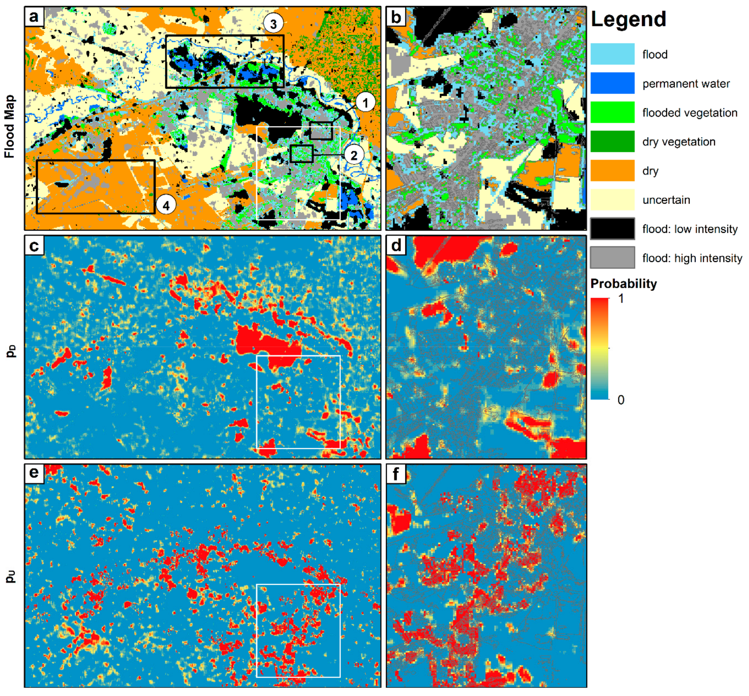
Figure 6a shows the mapping result at the cutoff probability of $p_D=0.5$ (black pixels) and $p_U=0.5$ (grey pixels). The largest open-water flood body (with a w-shape) near the central part of the AOI was well depicted. In the urban area (Figure 6b), we saw that a large proportion of the urban floods were mapped by the criterion of $p_U\ge 0.5$, indicating that these pixels experienced an intensity increase during the event epoch as compared with other epochs in their own history, and the increase was significant enough such that the probability of being flooded was over 50%. However, we could still observe that a visible portion of the urban flood could not be mapped by this p50-ts method (Figure 6b). The unmapped pixels represented flooded areas without significant changes of during-event backscattering in the time series. The mosaicking pattern of intensity decrease, intensity increase, and even unchanged intensity signified the complexity of radar backscattering patterns of floods in urban areas.

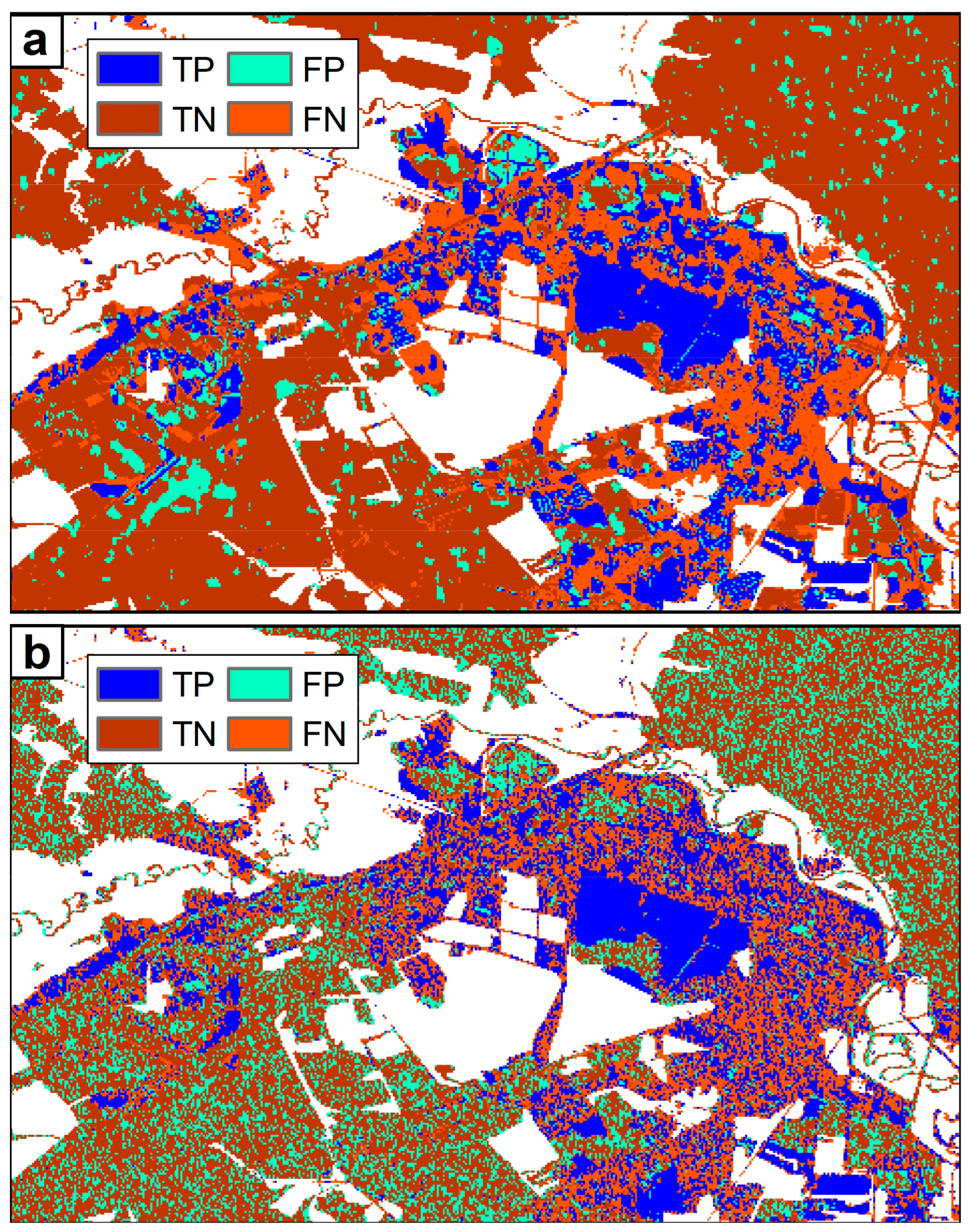
Next, we looked at the probability maps (Figure 6c–f). The transition zone of intermediate probability (yellow color) was narrow, with the majority of the mapped flood at the high probability end (p > 0.9; red color). The effect of underprediction was also demonstrated by having low probability values in the pixels within the Flood and Flooded Vegetation classes (Figure 6b vs. Figure 6d,f). Their spatial distributions were more clearly shown by the contingency map (Figure 7), where the mapped urban flood was mainly surrounded by FN pixels. Overprediction (FP pixels), on the other hand, was not as common within the urban area.

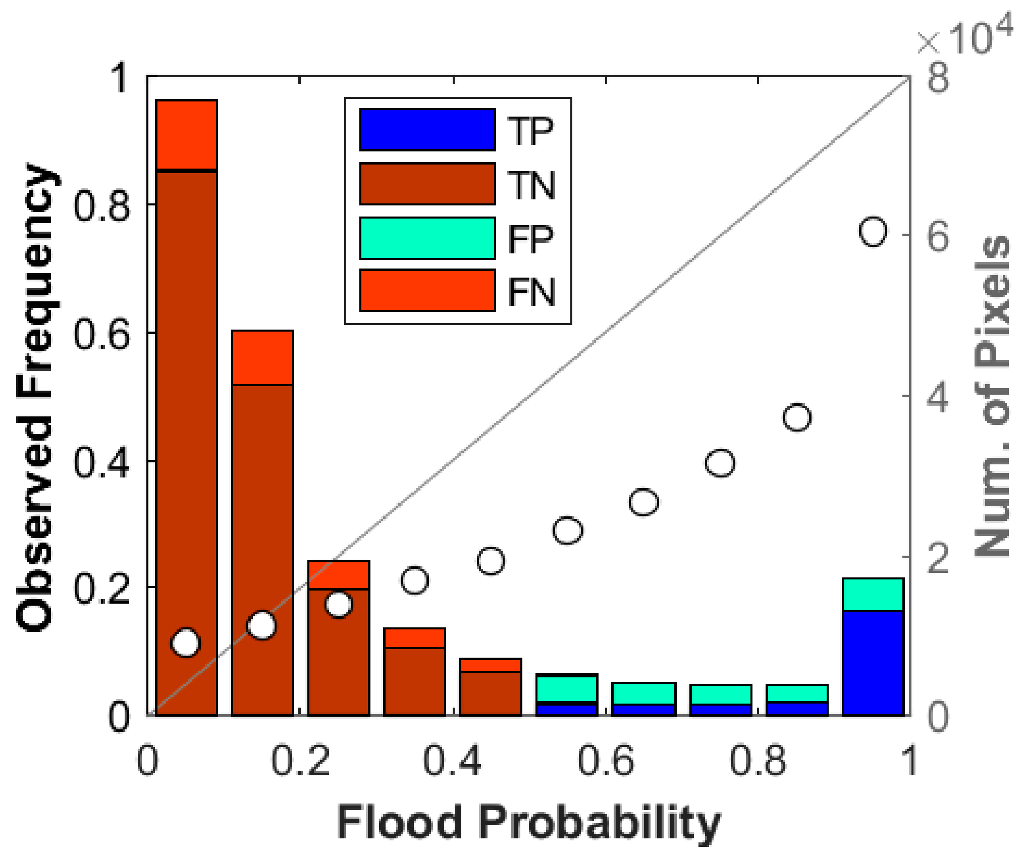
On the reliability diagram (Figure 8), we saw that the plots were mostly below the 1:1 line, with the flood probability larger than the observed frequency, except for the first and second bin ($p_F=0~0.2$). In the first bin, $p_o$ was mainly determined by FN/(FN+TN), so the ~5% higher in $p_o$ than $p_F$ came from the larger number of FN pixels than what $p_F$ predicted. In the last bin, $p_o$ was mainly determined by TP/(TP+FP), so the ~14% lower value in $p_o$ than $p_F$ came from the larger number of FP pixels than that predicted by $p_F$ (overprediction). It would be wrong to interpret the numbers as indicating that the mapping results suffered more overprediction than underprediction because the sample numbers varied greatly in each bin. The best way to view reliability is by looking at the weighted root-mean-square error between the plot and the 1:1 line ($\mathsf{\epsilon } \mathrm{in} \left(9\right)$), which was around 13%. This can be interpreted as the average error in the probability map.

The evaluation metrics echoed what we found in the maps and plots (

Table 2. Evaluation Metrics.

Type	Overall				Urban
	CSI+ [%]	OA+ [%]	PA+ [%]	UA+ [%]	CSI [%]	OA [%]	PA [%]	UA [%]
p50-ts method	34.4	80.8	45.5	56.7	40.2	42.8	43.4	83.3
Best result of grid search* on normalized ${\sigma }^0$	34.1	80.7	46.4	56.2	40.1	42.9	43.0	83.8
Best result of grid search* on log intensity ratio	24.0	64.2	51.9	30.5	41.3	44.6	44.3	85.2
p50-ts method (treating Flooded Veg. as nonflooded)	33.0	82.7	50.0	48.7	36.0	49.4	41.2	72.2

* Using overall critical success index (CSI) as the criterion. For reference purposes only. ⁺CSI = critical success index; OA = overall accuracy; PA = producer’s accuracy; UA = user’s accuracy

). The comparison with the best grid search result of the same normalized dataset showed that the p50-ts method could reach identical performance as the best choice of thresholds. When comparing with the best grid search result of log intensity ratio, we could see that the p50-ts method had higher overall CSI (34% vs. 24%) and OA (81% vs. 64%). There was a slight decrease in PA (~6%), but UA went from 30% for the log intensity ratio method to 57% for our technique, suggesting significant improvement in reducing the number of overpredicted (FP) pixels. In the urban area, the metrics from our method and the log intensity ratio method were similar, but the resulting flood maps showed different flood patterns (Figure 7). The difference was due to the fact that although global thresholds were used in both approaches, the time series normalization accounted for a certain level of spatial difference by considering the different history for each pixel; hence, the corresponding σ⁰ thresholds spatially varied.

In summary, the p50-ts method improved flood mapping in the case of Hurricane Matthew flood within the Lumberton area. The result is close to the best of what can be done with the optimal uniform thresholding on a pair of SAR images. However, the result still suffers obvious underprediction and overprediction. Next, we discuss the potential sources for the false predictions.

6. Discussion

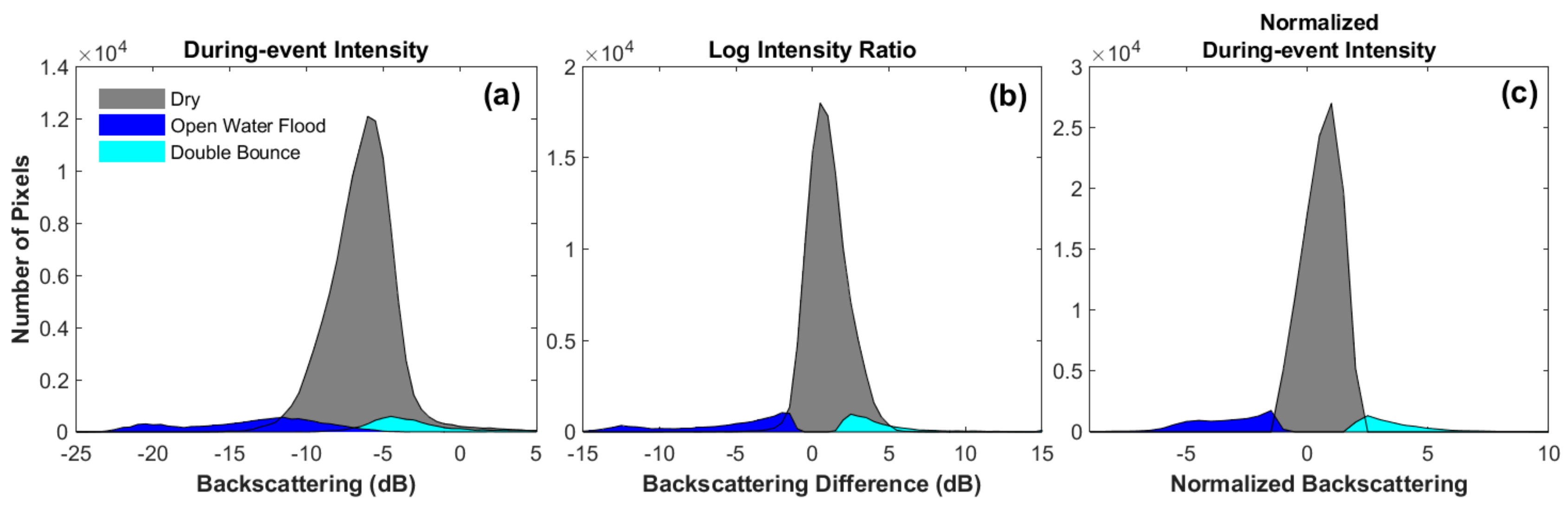
The time series normalization allows us to identify the flood-related double bounce pixels and specular reflection pixels of statistical significance. With that we can study the statistical distribution for these two effects. We sorted out the pixels that were in the Flood class and mapped as flooded due to intensity increase, and we interpreted these as due to double-bounce effect. We compared their histogram with histograms for (1) pixels in the Flood class mapped as flooded due to intensity decrease, interpreted as open water flood that saw specular reflection, and (2) pixels in the Dry class mapped as nonflooded. The plots in Figure 9 indicate that, from the histogram perspective, the normalized during-event intensity (Figure 9c) could better separate the pixels that saw double-bounce scattering than the log intensity ratio (Figure 9b). For the open water flood, the normalized during-event intensity and the log intensity ratio had similar efficacies in separating them from the nonflooded. The single during-event intensity (Figure 9a) had the worst histogram separation among all three. The better separation capability for double-bounce scattering marks the value of this method in studying urban floods.

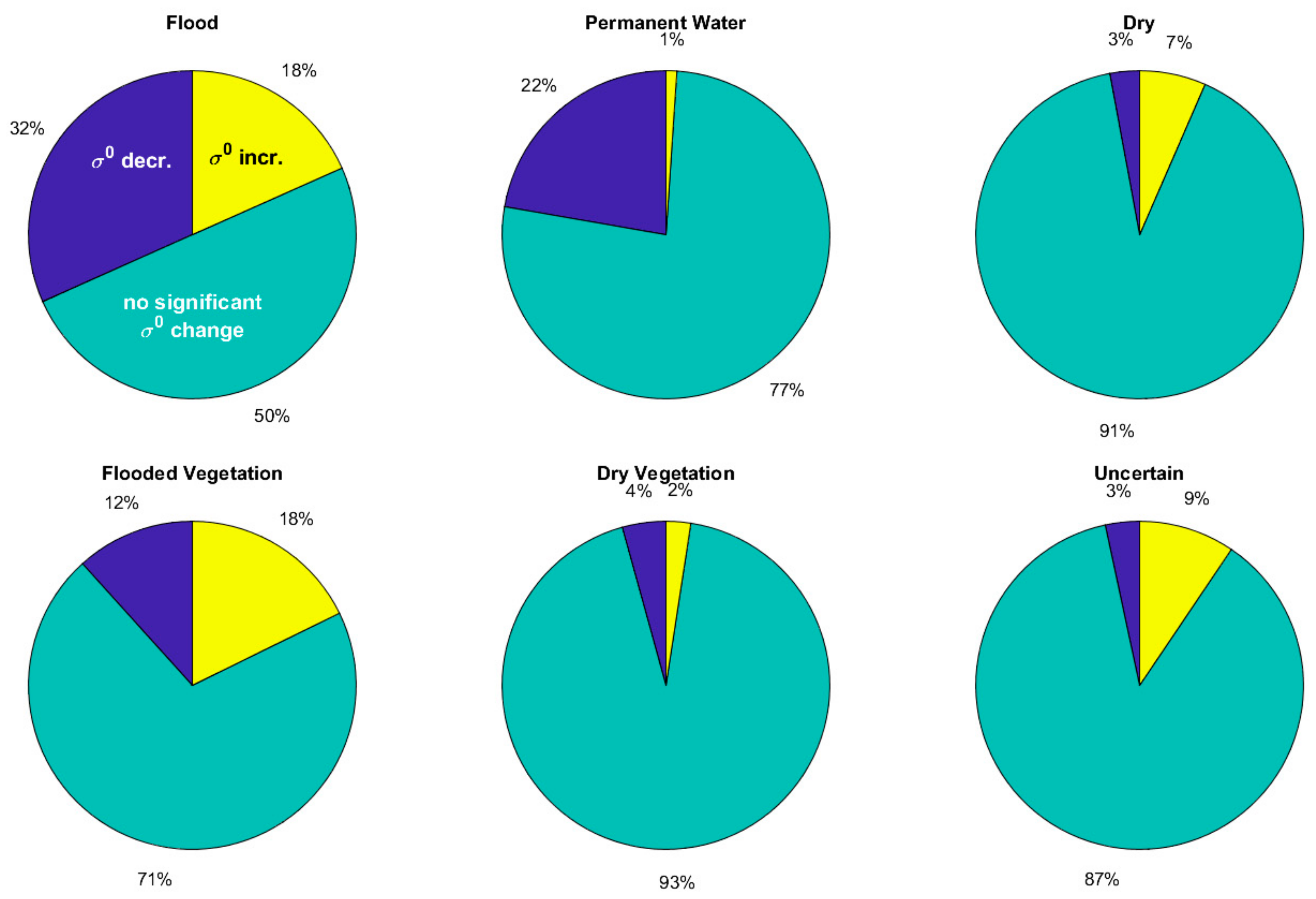
We also looked at the intensity changes with respect to the p50 threshold in the six validation classes individually (Figure 10). In the Flood class, only 50% of the pixels were detected as flood, among which 32% were identified with σ⁰ decrease and 18% with σ⁰ increase. In the remaining 50% there was no clear σ⁰ anomaly based on the thresholds given. In the Flooded Vegetation class, we saw more pixels with σ⁰ increase (18%) than those with σ⁰ decrease (12%). However, about 70% of the pixels in the Flooded Vegetation class did not see significant σ⁰ changes. In the Permanent Water class, 22% of the pixels were identified as flood by σ⁰ decrease. As for the Dry and Dry Vegetation classes, we saw a small fraction of false positives (6%–10%). Next, we would like to address the potential sources that cause the underprediction in the Flood and Flooded Vegetation class as well as the overprediction in the Permanent Water and Dry class.

6.1. Uncertainties in the Validation Dataset

One possible source of error is uncertainties in the validation dataset. We generated the validation data by rasterizing the validation vectors of ~30 cm resolution into 15 × 15 m pixels. At a regional scale, the rasterized image agreed in general with the vector file (Figure 2). However, when we zoomed in to the local scale, we observed discrepancies between the two (Figure 10a,b and Figure 11a,b). The discrepancies were associated with the sizes and orientations of the objects as well as their relative portion within a pixel. The difference was particularly obvious in a setting where the objects were densely distributed but isolated from one another. Thus, although the number of pixels falsely validated may only account for a small portion in the AOI, we should always be aware of the existence of such uncertainties, especially when utilizing moderate-resolution SAR images in flood mapping.

6.2. Source of Underprediction

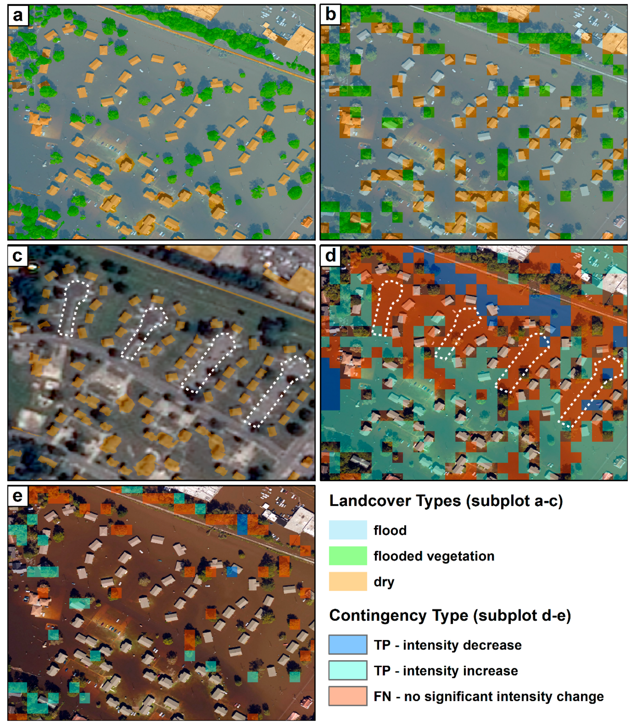
Underprediction (FN) accounted for the majority of false predictions. We first used patch 1 (Figure 6a) to discuss the possible sources of underprediction. In Figure 11d, there was a clear pattern of underprediction, with four elongated zones of FN subparallel to each other. According to the pre-flood optical image, these zones were asphalt roads (Figure 11c). Several studies have pointed out that asphalt will show up as dark pixels in radar images due to its smooth surface and low subsurface soil moisture content [32,33,34]. What we saw in this study was that the backscattering from asphalt surfaces could be as low as that from a water surface and, hence, indistinguishable from the during-event flood in the time series. This agrees with the point made by [6], that smooth surfaces such as tarmac, paved road, and parking lots may serve as water surface-like radar response areas. In the cases where they are actually flooded, there may not be any intensity anomaly compared to dry conditions. This is one of the major sources of underprediction.

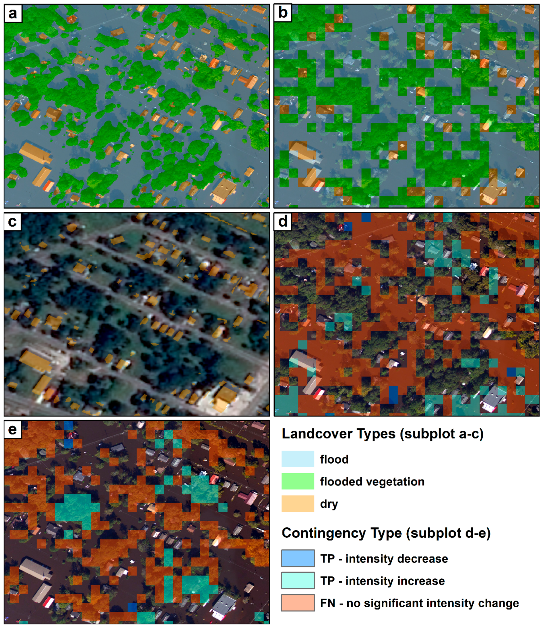
In patch 2, we saw another source of underprediction. This patch was inside a region with trees, houses, and parallel small roads. These densely packed houses and trees may cause serious shadow effects, leading to undetectable zones of constant low intensity (Figure 12c,d). Therefore, shadow was an effect that the time series normalization would not be able to deal with.

One thing worth pointing out is that shadow and smooth surfaces usually cause overprediction in the flood mapping with a single intensity image, while it causes underprediction in the log intensity ratio method as well as our time series normalization method.

There is one more phenomenon that drew our attention: only a small portion of the Flooded Vegetation was mapped as flooded (Figure 11e and Figure 12e). Some of the tree patches showed significant during-event intensity changes while others did not (Figure 11e). The logic behind the Flooded Vegetation class is that since the small tree patches were surrounded by open water flood, backscattering could be stronger when the radar wave penetrated the tree crown and reflected at the tree trunks and at the water surface, or vice versa. This expected behavior was, however, only seen in 18% of the Flooded Vegetation class, with another 12% seeing intensity decrease that could not be explained by the double-bounce mechanism. Therefore, despite the higher probability of observing intensity increase as compared with the Dry Vegetation class (Figure 10), it is likely that the backscattering for this class was the combination of changes in trees and flood. There is no easy way to separate the contribution from these two mechanisms. We had quickly tested to re-categorize this class as nonflooded, and this gave better overall OA (+2%) and PA (+4.5%) but lower CSI (−1.4%) and UA (−8%) (Table 2). As tree penetration capability is also a function of radar wavelength and polarization [35], there may not be a single answer to what would be the most appropriate way to validate the flood mapping in this class.

6.3. Source of Overprediction

A large proportion of overprediction (FP) was seen in the Permanent Water class (Figure 10). One example is in patch 3, where part of the pond water was mapped as flooded (Figure 13a-c). When we compared the pre-event and during-event optical images, we observed that some of the ponds were possibly vegetated with aquatic plants. As aquatic plants such as macrophytes are known to cause high backscattering intensity in C-band SAR [35], it is likely that we would see a during-event intensity decrease when the pond water level increased higher than the plants. Vegetation in the permanent waterbody is, therefore, one potential source of overprediction.

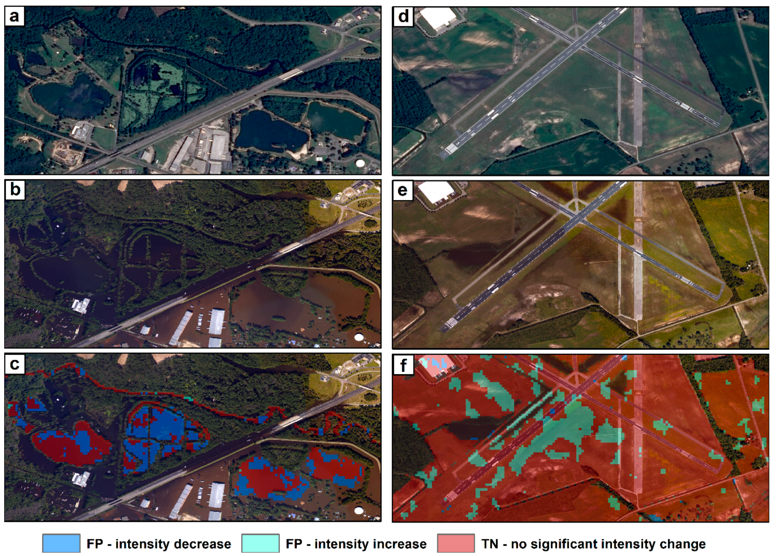
Another source of overprediction comes from the during-event intensity increase in the Dry class (Figure 11). One example is shown in patch 4, in which the soil underneath the sparse low meadow appeared darker in the during-event aerial image (Figure 12e) than the pre-event satellite image (Figure 12d); However, there was no water visible on the surface. This is a known effect of soil moisture, where the rise in soil moisture will also give rise to a radar backscattering intensity increase [36,37]. This effect is more obvious in bare soil or sparse meadow land cover types and, hence, affects more the prediction of rural floods than urban floods.

Finally, the increase in backscattering intensity from buildings, possibly due to cumulated water on the roof, also accounted for some overprediction in the Dry class, although the proportion was relatively small in this case study.

7. Conclusions

In this paper we presented an approach to utilize multitemporal SAR intensity information in a Bayesian probability framework for mapping floods in Lumberton, North Carolina, caused by the 2016 Hurricane Matthew. We normalized during-event SAR intensity observations with statistics from the SAR intensity time series, and we computed the flood probability with prior and likelihood functions. Flood detections based on a cutoff probability of 0.5 showed improved performance when compared with results from an approach that used the optimal uniform threshold in pre- and during-SAR intensity pair analyses. The mapping result showed that a high percentage of the urban flood was associated with SAR intensity increase (double-bounce effect), and the urban flood in Lumberton was a complicated mosaic of pixels, with during-event intensity increase and intensity decrease as well as pixels without significant intensity changes. Underprediction was as high as 50%, which we interpreted to be mainly associated with asphalt surface cover and shadow effects. Overprediction is possibly related to vegetation in permanent water bodies and local soil moisture increase.

References

1. Sentinel Asia. Sentinel Asia Sentinel Asia Annual Report 2017; Japan Aerospace Exploration Agency: Tokyo, Japan, 2019; p. 48. [Google Scholar]
2. Mason, D.C.; Speck, R.; Devereux, B.; Schumann, G.J.P.; Neal, J.C.; Bates, P.D. Flood detection in urban areas using TerraSAR-X. IEEE Trans. Geosci. Remote Sens. 2010, 48, 882–894. [Google Scholar] [CrossRef]
3. Ferro, A.; Brunner, D.; Bruzzone, L.; Lemoine, G. On the Relationship between Double Bounce and the Orientation of Buildings in VHR SAR Images. IEEE Geosci. Remote Sens. Lett. 2011, 8, 612–616. [Google Scholar] [CrossRef]
4. Pulvirenti, L.; Chini, M.; Pierdicca, N.; Boni, G. Use of SAR data for detecting floodwater in urban and agricultural areas: The role of the interferometric coherence. IEEE Trans. Geosci. Remote Sens. 2016, 54, 1532–1544. [Google Scholar] [CrossRef]
5. Mason, D.C.; Davenport, I.J.; Neal, J.C.; Schumann, G.J.P.; Bates, P.D. Near real-time flood detection in urban and rural areas using high-resolution synthetic aperture radar images. IEEE Trans. Geosci. Remote Sens. 2012, 50, 3041–3052. [Google Scholar] [CrossRef]
6. Giustarini, L.; Hostache, R.; Matgen, P.; Schumann, G.J.P.; Bates, P.D.; Mason, D.C. A change detection approach to flood mapping in urban areas using TerraSAR-X. IEEE Trans. Geosci. Remote Sens. 2013, 51, 2417–2430. [Google Scholar] [CrossRef]
7. Pulvirenti, L.; Pierdicca, N.; Chini, M.; Guerriero, L. An algorithm for operational flood mapping from synthetic aperture radar (SAR) data using fuzzy logic. Nat. Hazards Earth Syst. Sci. 2011, 11, 529–540. [Google Scholar] [CrossRef]
8. Mason, D.C.; Giustarini, L.; Garcia-Pintado, J.; Cloke, H.L. Detection of flooded urban areas in high resolution Synthetic Aperture Radar images using double scattering. Int. J. Appl. Earth Obs. Geoinf. 2014, 28, 150–159. [Google Scholar] [CrossRef] [Green Version]
9. Tanguy, M.; Chokmani, K.; Bernier, M.; Poulin, J.; Raymond, S. River flood mapping in urban areas combining RADARSAT-2 data and flood return period data. Remote Sens. Environ. 2017, 198, 442–459. [Google Scholar] [CrossRef]
10. Chini, M.; Pelich, R.; Pulvirenti, L.; Pierdicca, N.; Hostache, R.; Matgen, P. Sentinel-1 InSAR Coherence to Detect Floodwater in Urban Areas: Houston and Hurricane Harvey as a Test Case. Remote Sens. 2019, 11, 107. [Google Scholar] [CrossRef]
11. Li, Y.; Martinis, S.; Wieland, M. Urban flood mapping with an active self-learning convolutional neural network based on TerraSAR-X intensity and interferometric coherence. ISPRS J. Photogramm. Remote Sens. 2019, 152, 178–191. [Google Scholar] [CrossRef]
12. Chaabani, C.; Chini, M.; Abdelfattah, R.; Hostache, R.; Chokmani, K. Flood Mapping in a Complex Environment Using Bistatic TanDEM-X/TerraSAR-X InSAR Coherence. Remote Sens. 2018, 10, 1873. [Google Scholar] [CrossRef]
13. Hostache, R.; Matgen, P.; Wagner, W. Change detection approaches for flood extent mapping: How to select the most adequate reference image from online archives? Int. J. Appl. Earth Obs. Geoinf. 2012, 19, 205–213. [Google Scholar] [CrossRef]
14. Schlaffer, S.; Matgen, P.; Hollaus, M.; Wagner, W. Flood detection from multi-temporal SAR data using harmonic analysis and change detection. Int. J. Appl. Earth Obs. Geoinf. 2015, 38, 15–24. [Google Scholar] [CrossRef]
15. Schlaffer, S.; Chini, M.; Giustarini, L.; Matgen, P. Probabilistic mapping of flood-induced backscatter changes in SAR time series. Int. J. Appl. Earth Obs. Geoinf. 2017, 56, 77–87. [Google Scholar] [CrossRef]
16. Addabbo, A.D.; Refice, A.; Pasquariello, G.; Lovergine, F.P.; Capolongo, D.; Manfreda, S. A Bayesian network for flood detection combining SAR imagery and ancillary data. IEEE Trans. Geosci. Remote Sens. 2016, 54, 3612–3625. [Google Scholar] [CrossRef]
17. Clement, M.A.; Kilsby, C.G.; Moore, P. Multi-temporal synthetic aperture radar flood mapping using change detection. J. Flood Risk Manag. 2018, 11, 152–168. [Google Scholar] [CrossRef]
18. Ouled Sghaier, M.; Hammami, I.; Foucher, S.; Lepage, R. Flood extent mapping from time-series sar images based on texture analysis and data fusion. Remote Sens. 2018, 10, 237. [Google Scholar] [CrossRef]
19. Stewart, S.R. Tropical Cyclone Report: Hurricane Matthew; National Hurricane Center: Miami, FL, USA, 2017; p. 96. [Google Scholar]
20. National Geodetic Survey, Remote Sensing Division (Data Producer). Hurricane Matthew: Rapid Response Imagery of the Surrounding Regions; OAA’s Ocean Service: Silver Spring, MD, USA, 2016.
21. Farr, T.G.; Rosen, P.A.; Caro, E.; Crippen, R.; Duren, R.; Hensley, S.; Kobrick, M.; Paller, M.; Rodriguez, E.; Roth, L.; et al. The Shuttle Radar Topography Mission. Rev. Geophys. 2007, 45. [Google Scholar] [CrossRef] [Green Version]
22. Miranda, N.; Meadows, P.J. Radiometric Calibration of S-1 Level-1 Products Generated by the S-1 IPF; ESA-EOPG-CSCOP-TN-0002; European Space Agency: Paris, France, 2015. [Google Scholar]
23. Jong-Sen, L.; Papathanassiou, K.P.; Ainsworth, T.L.; Grunes, M.R.; Reigber, A. A new technique for noise filtering of SAR interferometric phase images. IEEE Trans. Geosci. Remote Sens. 1998, 36, 1456–1465. [Google Scholar] [CrossRef]
24. Jong-Sen, L.; Grunes, M.R.; Grandi, G.D. Polarimetric SAR speckle filtering and its implication for classification. IEEE Trans. Geosci. Remote Sens. 1999, 37, 2363–2373. [Google Scholar] [CrossRef]
25. Pathe, C.; Wagner, W.; Sabel, D.; Doubkova, M.; Basara, J.B. Using ENVISAT ASAR global mode data for surface soil moisture retrieval over Oklahoma, USA. IEEE Trans. Geosci. Remote Sens. 2009, 47, 468–480. [Google Scholar] [CrossRef]
26. Huffman, G.; Bolvin, D.; Braithwaite, D.; Hsu, K.; Joyce, R.; Xie, P. Integrated Multi-Satellite Retrievals for GPM (IMERG), Version 4.4; NASA’s Precipitation Processing Center: Washington, DC, USA, 2014. [Google Scholar]
27. Hetland, E.A.; Musé, P.; Simons, M.; Lin, Y.N.; Agram, P.S.; DiCaprio, C.J. Multiscale InSAR Time Series (MInTS) analysis of surface deformation. J. Geophys. Res. 2012, 117. [Google Scholar] [CrossRef]
28. Riel, B.; Simons, M.; Agram, P.; Zhan, Z. Detecting transient signals in geodetic time series using sparse estimation techniques. J. Geophys. Res. 2014, 119, 5140–5160. [Google Scholar] [CrossRef] [Green Version]
29. Giustarini, L.; Hostache, R.; Kavetski, D.; Chini, M.; Corato, G.; Schlaffer, S.; Matgen, P. Probabilistic Flood Mapping Using Synthetic Aperture Radar Data. IEEE Trans. Geosci. Remote Sens. 2016, 54, 6958–6969. [Google Scholar] [CrossRef]
30. Marquardt, D. An Algorithm for Least-Squares Estimation of Nonlinear Parameters. J. Soc. Ind. Appl. Math. 1963, 11, 431–441. [Google Scholar] [CrossRef]
31. Chini, M.; Hostache, R.; Giustarini, L.; Matgen, P. A hierarchical split-based approach for parametric thresholding of SAR images: Flood inundation as a test case. IEEE Trans. Geosci. Remote Sens. 2017, 55, 6975–6988. [Google Scholar] [CrossRef]
32. Landuyt, L.; Wesemael, A.V.; Schumann, G.J.; Hostache, R.; Verhoest, N.E.C.; Coillie, F.M.B.V. Flood Mapping Based on Synthetic Aperture Radar: An Assessment of Established Approaches. IEEE Trans. Geosci. Remote Sens. 2019, 57, 722–739. [Google Scholar] [CrossRef]
33. Aronica, G.; Bates, P.D.; Horritt, M.S. Assessing the uncertainty in distributed model predictions using observed binary pattern information within GLUE. Hydrol. Process. 2002, 16, 2001–2016. [Google Scholar] [CrossRef]
34. Wilks, D.S. Statistical Metods in the Atmospheric Sciences, 3rd ed.; Elsevier, Academic Press: Oxford, UK, 2011. [Google Scholar]
35. Hess, L.L.; Melack, J.M.; Filoso, S.; Wang, Y. Delineation of inundated area and vegetation along the Amazon floodplain with the SIR-C synthetic aperture rada. IEEE Trans. Geosci. Remote Sens. 1995, 33, 896–904. [Google Scholar] [CrossRef]
36. Paloscia, S.; Pettinato, S.; Santi, E.; Notarnicola, C.; Pasolli, L.; Reppucci, A. Soil moisture mapping using Sentinel-1 images: Algorithm and preliminary validation. Remote Sens. Environ. 2013, 134, 234–248. [Google Scholar] [CrossRef]
37. Susan Moran, M.; Hymer, D.C.; Qi, J.; Sano, E.E. Soil moisture evaluation using multi-temporal synthetic aperture radar (SAR) in semiarid rangeland. Agric. For. Meteorol. 2000, 105, 69–80. [Google Scholar] [CrossRef] [Green Version]
Figure 1. Lumberton in Robeson County, North Carolina, and the during-event airborne optical imagery taken on 11 October 2016. The Lumber River flows right through the middle of the town. USC00315177 is National Oceanic and Atmospheric Administration (NOAA)’s ground weather station.
Remotesensing 11 01778 g001
Figure 2. (a) The during-event aerial image and (b) the validation vector image with 30 cm resolution. (c) The rasterized validation image at 15 m resolution. (d) The during-event Sentinel-1 synthetic aperture radar (SAR) image at 15 m posting. The cyan box indicates the region used for Gaussian curve fitting. (e,f) The magnified views of (ad) for the urban area. The open circles labeled 1 to 6 in (b) are the sample pixels of the time series (Figure 4) for each class.
Remotesensing 11 01778 g002
Figure 3. The processing flow chart for the intensity stack and flood proxy map. JPL ISCE, Jet Propulsion Laboratory’s InSAR Scientific Computing Environment.
Remotesensing 11 01778 g003
Figure 5. (a) The histogram and 2-Gaussian curve fitting for the during-event epoch in the normalized time series. (b) The curve fitting for 3-Gaussian model. RMSE = root-mean-square error. (c) The probability for the nonflooded, the flooded with intensity decrease, and the flooded cases, with intensity increase for the normalized backscattering in the time series. (d) The conditional probability of the normalized backscattering in the time series being flooded with intensity decrease (blue curve) or intensity increase (cyan curve). Black line with arrow indicates the cutoff threshold of p = 0.5 for a binary flood map.
Remotesensing 11 01778 g005
Figure 6. Flood mapped by the probability threshold of p = 0.5 for (a) the whole area of interest (AOI) and (b) the urban area. The second and third panels are for the probability maps of (cd) intensity decrease ( p D ) and (ef) intensity increase ( p U ). Numbers in white circles are the patch IDs used in discussion.
Remotesensing 11 01778 g006
Figure 7. Comparison between (a) the contingency map obtained by p = 0.5 cutoff threshold and (b) the contingency map from the best result of grid search on log intensity ratio of during- and pre-event image (i.e., nontemporal analysis). Pixels in the Uncertain class are masked out from the map.
Remotesensing 11 01778 g007
Figure 8. The reliability diagram between the flood probability p F and the observed frequency p o (white circles). The number of pixels for each probability bin is shown in vertical bars color-coded by contingency types. The deviation of the circles from the 1:1 line represents the error for each probability bin. The pixel counts in different contingency types shows that the error comes from FN (underprediction) for probability bins below 0.5, and FP (overprediction) for probability bins above 0.5.
Remotesensing 11 01778 g008
Figure 9. The histogram comparison between the pixels in the Dry class and mapped as nonflooded (grey), Flood class and mapped as flooded with intensity decrease (cyan, interpreted as open water flood), and Flood class and mapped as flood with intensity increase (cyan, interpreted as double bounce scattering). (a) Histogram for the pixel during-event intensity. (b) Histogram for the pixel log intensity ratio. (c) Histogram for the pixel during-event intensity after time-series normalization.
Remotesensing 11 01778 g009
Figure 10. Pie charts showing, for each of the 6 classes, the proportions of pixels detected as flooded with either σ0 decrease (blue) or σ0 increase (yellow), or as nonflooded with insignificant σ0 change at the p50 thresholds.
Remotesensing 11 01778 g010
Figure 11. The during-event aerial photo for patch 1 (see Figure 6a for location), overlaid with (a) the land cover classes in vector format, and (b) the rasterized land cover map in 15 × 15m resolution. (c) The pre-event satellite image overlaid with the Dry class for reference. The white dashed lines represent asphalt driveways. (d) The contingency map for the Flood class. (e) The contingency map for the Flooded Vegetation class.
Remotesensing 11 01778 g011
Figure 12. Same caption as Figure 10 but for patch 2. See Figure 6a for location.
Remotesensing 11 01778 g012
Figure 13. The (a) pre-event optical image and (b) during-event aerial photo for patch 3. See Figure 6a for location. (c) The contingency map for the Flood class. (de) Same as (ab) for patch 4. (f) The contingency map for the Dry class.
Remotesensing 11 01778 g013