Field-Scale Crop Seeding Date Estimation from MODIS Data and Growing Degree Days in Manitoba, Canada

Abstract

Information on crop seeding date is required in many applications such as crop management and yield forecasting. This study presents a novel method to estimate crop seeding date at the field level from time-series 250-m Moderate Resolution Imaging Spectroradiometer (MODIS) data and growing degree days (GDD; base 5 °C; °C-days). The start of growing season (SOS) was first derived from time-series EVI2 (two-band Enhanced Vegetation Index) calculated from a MODIS 8-day composite surface reflectance product (MOD09Q1; Collection 6). Based on GDD calculated from the Daymet gridded estimates of daily weather parameters, a simple model was developed to establish a linkage between the observed seeding date and the SOS. Calibration and validation of the model was conducted on three major crops, spring wheat, canola and oats in the Province of Manitoba, Canada. The estimated SOS had a strong linear correlation with the observed seeding date; with a deviation of a few days depending on the year. The seeding date of the three crops can be calculated from the SOS by adjusting the number of days needed to accumulate GDD (AGDD) for emergence. The overall root-mean-square-difference (RMSD) of the estimated seeding date was less than 10 days. Validation showed that the accuracy of the estimated seeding date was crop-type independent. The developed method is useful for estimating the historical crop seeding date from remote sensing data in Canada to support studies of the interactions among seeding date, crop management and crop yield under climate change. It is anticipated that this method can be adapted to other crops in other locations using the same or different satellite data.

1. Introduction

Seeding date is an important factor influencing the development and productivity of field crops. Planting crops within an optimal time window could avoid the negative impact of unfavorable environmental conditions on crop development, and therefore maximize crop yield [1,2,3,4]. Seeding date is also one of the most important parameters in modelling crop yield, and crop response to agricultural management practices and climate variability [4,5,6]. Seeding date varies annually and spatially depending on the variation in weather conditions and soil characteristics. Due to difficulties in obtaining seeding-date information directly, various estimation methods have been developed and reported in the literature [7,8].

Remote sensing (RS) technology has the advantage of providing a synoptic view of crop development over large areas [9,10,11]. Estimation of crop phenological metrics using RS data depends largely on greenness information captured by optical satellite sensors. Studies have found that remotely sensed crop phenological metrics, especially the start of growing season (SOS, green-up date), can provide spatially explicit information on crop development stages, including the seeding date [7,12,13]. Crop phenological metrics are usually derived from time-series vegetation indices (VIs) through curve fitting, and the indices are usually calculated from reflectance data in the visible and near-infrared (NIR) bands. The Normalized Difference Vegetation Index (NDVI), the Enhanced Vegetation Index (EVI), and the two-band EVI without a blue band (EVI2) [11,14,15] are common VIs. In general, the SOS derived from optical satellite data is close to the earliest time of vegetation growth, such as leaf emergence [11,16,17]. For example, the SOS is commonly defined as the date when VIs reach a threshold level of about 10–20% of the seasonal maximum amplitude [15,16]. Methods using the inflection point of a VI curve at the growing phase are also widely used for SOS estimation, as the inflection point is found to correspond to the onset of rapid vegetative growth [11]. As a result, the SOS responds to actual growth stages; however, the specific relationship varies with the methods used [17,18,19].

To estimate seeding date based on SOS derived from time-series remote sensing data, a constant number of days ranging from seven days to three weeks have been reported in the literature [13,20,21]. For instance, Lobell et al. [13] employed a fixed 3-week period to obtain spatially explicit seeding date of wheat in India from SOS defined with a 10% threshold level of seasonal maximum NDVI. This fixed value was determined using simulations of the CERES-Wheat model. Vyas et al. [21] also estimated the seeding date of wheat in India by subtracting seven days from the date of the inflection point of the NDVI time series at the vegetative phase. While using a constant number of days to estimate seeding date from remotely sensed SOS has the benefit of simplicity, it could also induce bias. As the duration between the seeding date and the emergence date depends on soil texture, temperature, soil water, planting depth and their interactions [22,23,24], the time-lag could be longer in a cool year than in normal years [22,25]. Thus, the duration between the seeding date and SOS can vary with geographical location, crop management practices, climate variability, crop type, and cultivar of the same crop type [8,24]. To address these uncertainties, more complex methods have been developed to better capture the relationship between the remotely sensed SOS and seeding date. Manfron et al. [8] proposed a rule-based method to estimate the inter-annual variability of seeding dates in winter wheat in Camargue, France. This rule-based method was built on agronomist’s knowledge of the temporal signatures of winter wheat, such as the seeding window and the time required reaching the 3-leaf stage. In a global study by Kotsuki et al. [18], the threshold value of NDVI for estimating the seeding date was calibrated using census data from three consecutive years for six crops. Their results showed that the threshold NDVI value for determining SOS varied with crop type but not with spatial location or year. Ortiz-Monasterio et al. [26] found that the seeding date of spring wheat could be estimated well, with an error of 6.5 days, when the fraction of absorbed photosynthetically active radiation (fAPAR) estimated from two Landsat ETM+ images was assimilated into a wheat growth model. This study demonstrated the potential of seeding-date estimation by assimilating time series remotely sensed biophysical parameters (e.g., leaf area index (LAI) and fAPAR) into crop growth models. However, most crop growth models require data inputs that are difficult to obtain from either ground measurements or satellite observations, making the method difficult to implement over large areas. Similar to the agrometeorological approach to be discussed in the next section, all these methods have highlighted that the length of the period from seeding date to a specific crop development stage is affected by climate variability.

Predicting crop growth stages, such as leaf emergence, from seeding date based on agrometeorological data has been the most commonly used method [27,28]. This approach usually requires agrometeorological data such as air temperature and precipitation. In particular, the accumulated daily temperature above a base temperature (the growing degree days, GDD, °C -days) needs to be integrated into crop growth models [5,22,23]. A specific crop development stage will start when the accumulated GDD (AGDD) reaches a certain threshold window [22,23,29]. A linear relationship between crop development stages and AGDD has been reported for various crops in different regions [5,30,31]. For example, Mkhabela et al. [32] found that a simple GDD model performed the best among three thermal time models (the North-Dakota GDD, the GDD with base temperature of 0 °C and the GDD with base temperature of 5 °C) for predicting spring wheat phenology in western Canada. Saiyed et al. [31] reported that the thermal time models, including the GDD information and biometeorological time scale (BMT, involving both temperature and photoperiod), were effective in estimating the days required for spring wheat to reach anthesis and maturity from seeding date in western Canada. Chang et al. [5] showed that the capability for simulating crop phenology and crop carbon cycle was improved when a simple GDD-based phenology algorithm was integrated into the Carbon and Nitrogen-Coupled Canadian Land Surface Scheme (CN-CLASS). Several global datasets for major crop seeding dates, such as those highlighted in Sacks et al. [3] and Waha et al. [33], have been developed based on an agrometeorological approach. All of these studies have highlighted the importance of thermal-time variability to crop development. This agrometeorological approach is highly dependent on the availability of nearby weather stations, while in reality station networks tend to be quite sparse, and the estimation of crop development stages is poor over areas where there are no nearby weather stations. In this case, the estimated crop development stage is insufficient for field-scale crop modelling and management over large areas [12,34].

In light of the benefits of remote sensing and agrometeorology-based methods, seeding date could be better estimated over large areas using a combination of these methods, rather than using a single method alone. The usefulness of GDD has been demonstrated in a wide range of RS studies. The accuracy of crop classification [35,36], crop yield estimation [37], and crop phenology extraction [19] have all been shown to be effectively improved when the GDD information was used with RS data. The overall objective of this study was to estimate crop seeding date from MODIS 250-m time-series data products combined with GDD information. Specific objectives include: (1) estimating start of growing season from 250-m MODIS data products; (2) investigating the relationship between remotely sensed SOS and real seeding date for different crops and years; and (3) developing an approach to estimate seeding date at the field level from remotely sensed SOS combined with GDD information. The proposed approach was evaluated over agricultural regions in the Province of Manitoba, Canada, and observed seeding dates for the years of 2006 and 2009, with large difference in meteorological conditions between the two years, were used. In particular, suitability of the approach for different years and for different crops is assessed.

2. Materials and Methods

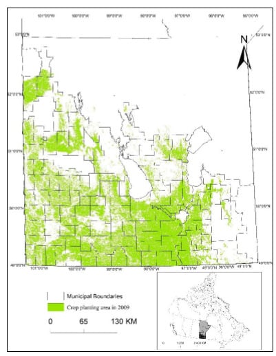
2.1. Study Area

Manitoba has a relatively large agricultural area, mostly distributed in the southern portion of the province bordering the United States (Figure 1). The region has a sub-humid continental climate and is characterized by cold and windy winters and warm, moderately long summers. Soil type is dominated by Black and Dark Gray Chernozems and Gray Luvisols [38]. Total rainfall and average daily mean temperature during the crop growing season (May 1–September 30) is more than 300 mm and about 15 °C, respectively [39]. Canola, spring wheat, oats, barley and flaxseed, are the five major annual crops of the province, comprising more than 90% of the cropped area (Manitoba Agriculture, Food and Rural Initiatives, MAFRI, https://www.gov.mb.ca/agriculture). Single-season cropping is the primary practice, with crops generally seeded from late April to mid-June and harvested starting in mid-August (Seasonal Reports, MAFRI, https://www.gov.mb.ca/agriculture). This study was conducted using two years of data (2006 and 2009) with varying weather conditions.

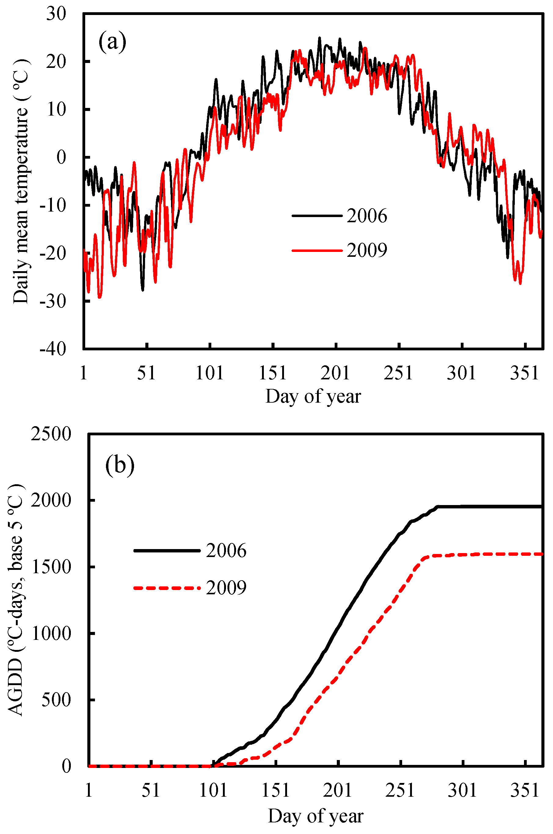
2.2. Air Temperature Data

The minimum and maximum daily temperature from January 1 to December 31 of each year were derived from the Daymet Version 3 daily gridded data in the Oak Ridge National Laboratory (ORNL) Distributed Active Archive Center (DAAC) [40]. The main inputs of the Daymet model are surface observations from the Global Historical Climatology Network (GHCH)-Daily dataset distributed by the National Centers for Environmental Information (NCEI). The daily outputs of the Daymet model cover North America at a 1-km spatial resolution. The outputs include minimum and maximum temperature, precipitation, shortwave radiation, vapor pressure, snow water equivalent, and day length. To match the spatial resolution and the projection system of the MODIS data, the temperature data was resampled to the same spatial resolution (250-m) of the MODIS data using a bilinear resampling method. The daily mean temperature in 2009, especially during the early season before July, was cooler than in 2006; therefore, the AGDD (base 5 °C) in 2006 was higher than in 2009 (Figure 2). Crop growth and development in 2006 was therefore different from that in 2009.

2.3. Observed Seeding Date

Crop seeding date was obtained from the crop insurance data of Manitoba provided by the Manitoba Agricultural Services Corporation. In this dataset, crops are recorded for “quarter section”, a land surveying geographical boundary used in the Canadian Prairie provinces. A quarter section is about 800 m × 800 m (640,000 m²), covering about 10 250-m MODIS pixels. The quarter section is a part of the hierarchy of Dominion Land Survey in the Canadian Prairies. The geographical boundary of many agricultural fields in Manitoba follows the outlines of the Dominion Land Survey units (i.e., quarter sections, parts of quarter sections or a combination of multiple quarter sections). A large number of quarter sections are seeded with a single crop. Seeding depth and rate of each crop are conducted based on the guides of field crop management practices provided by the MAFRI. They therefore are assumed to be uniform within field and between fields. Seeding date is generally between May 1 and May 31 for spring wheat, May 1 and June 20 for canola, and May 1 and June 10 for oats (Seasonal Reports, MAFRI, https://www.gov.mb.ca/agriculture). The seeding date for 2006 and 2009 were used in this study because of the large difference of daily mean air temperature in the two years.

2.4. MODIS Data

Time series EVI2 was used in deriving crop phenological metrics; compared with other VIs, EVI2 is less sensitive to the influence of canopy background reflectance at low LAI [41,42,43]. Previous studies have shown that the extraction of phenological metrics from EVI2 is more robust [14,44]. To derive EVI2 time series, the MOD09Q1 (Collection 6) data covering the agricultural region of Manitoba (MODIS titles: h12v03, h11v04 and h11v03) was downloaded from the Earth Science Discovery Tool of NASA (https://search.earthdata.nasa.gov/). The MOD09Q1 provides 8-day composite surface reflectance in the red and NIR bands. Each pixel value represents the best quality observation during the 8-day period. The layers of the two bands and the QC (Quality Control) were extracted and re-projected to UTM projection (Zone 14N) using the MODIS Reprojection Tool (MRT). The EVI2 (Equation (1)) was then calculated from the reflectance of the two bands.

$$\mathrm{EVI}2=\frac{2.5\left(\mathrm{NIR}-\mathrm{RED}\right)}{\left(\mathrm{NIR}+2.4\mathrm{RED}+1.0\right)}.$$

(1)

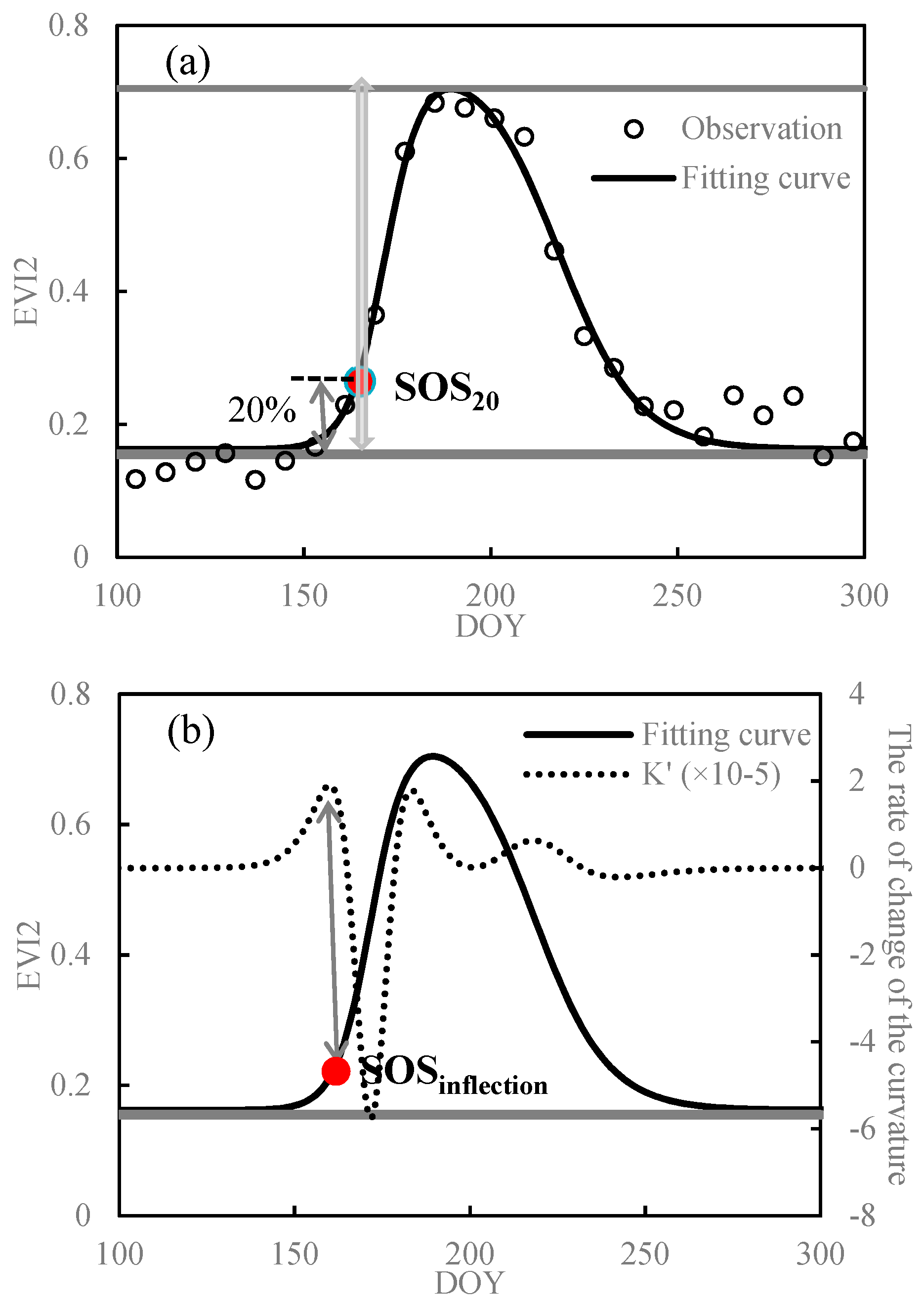
2.5. Extraction of SOS from EVI2

Two steps were involved in deriving the remotely sensed SOS. The first step was to reconstruct daily EVI2. Low-quality observations caused by cloud, aerosol, snow cover and other factors were first filtered out based on the QC (Quality Control) value provided by the MOD09Q1 product. The study area has a long winter, and crop growing season is generally between May and September. EVI2 in the winter season may be negative because of snow cover, thus, EVI2 between late March (DOY 90) and late October (DOY 300) were selected. Observations below 0.05 among the remaining selections were excluded as well. A time-series fitting model was then used to further de-noise and rebuild daily EVI2. The Parametric Double Hyperbolic Tangent (PDHT) mathematic model was employed to fit the daily EVI2 in order to derive phenological indicators. It has proven to be well suited for reconstruction of daily fAPAR in the Canadian Prairies [45]. The fitted daily EVI2 can be expressed as:

$$EVI2\left(t\right)=a_0+\frac{a_1\left\{\tanh \left[\left(t-a_2\right)a_3\right]+1\right\}}{2}+\frac{a_4\left\{\tanh \left[\left(t-a_5\right)a_6\right]+1\right\}}{2}-a_4.$$

(2)

where t is the day of year (DOY); a₀ is the minimum EVI2 value corresponding to bare soil; a₁ and a₄ define the amplitude of EVI2 for the vegetative and the reproductive phases, respectively; a₂ and a₅ allow shifting the inflection points of the vegetative and reproductive phases along the time axis, respectively; and a₃ and a₆ define the slopes of the vegetative and reproductive phases, respectively. The optimal parameters of PDHT were achieved based on the Levenberg-Marquardt algorithm [46]. Based on the fitted daily EVI2, the threshold-based and inflection-based approaches, two broadly used methods for phenological metrics extraction [15,47], were employed to estimate two sets of SOS.

i. For the threshold-based method, the SOS is defined as the time during vegetation growth phase when EVI2 increases to a given threshold level [16,48,49]. In this study, the threshold level was set to 20% of the seasonal EVI2 amplitude (SOS₂₀, Figure A1), i.e., the difference of the maximum and minimum EVI2 in a growing season [15,50].

ii. For the inflection-based method, Zhang et al. [11] defined the date of phenological stage (e.g., SOS) as representing the transition of vegetation development from one approximately linear growth stage to another. Therefore, phenological metrics can be extracted based on the change of curvature (K) [11]. For the inflection-based method, the green-up date in this study (SOS_inflection, Figure A1) was considered as the inflection point corresponding to the first local maximum of the first-order derivative of the curvature [11]. The K can be calculated using the following equation (Equation (3)).

$$K=\frac{y^{″}}{{\left(1+{\left(y^{\prime }\right)}^2\right)}^{\raisebox{1ex}{$3$}\!\left/ \!\raisebox{-1ex}{$2$}\right.}}.$$

(3)

where y′ and y″ are the first-order and second-order derivatives of the daily EVI2, respectively.

2.6. Model for Estimating Seeding Date from SOS

To reduce the influence of pixel-mixing and other factors on establishing models for estimating seeding date from SOS, representative samples were selected firstly. Quarter sections with seeding date observation satisfying the following two conditions were selected:

(1) They were fully covered by a single crop. This excludes the pixel-mixing effect within a quarter section;

(2) Median SOS of the pixels within a quarter section was determined to represent SOS of the quarter section. This can exclude quarter sections with relatively large difference of SOS for the MODIS pixels. This is to obtain a more satisfactory curve fitting by excluding some of the low quality EVI2 data. Even though a crop within a quarter section is generally seeded all on the same day, crop development early in the season may not be uniform within a quarter section with large within-field variability in soil properties, soil moisture or elevation [6,51,52].

After determining samples for each crop and year, the linear relationship between remotely sensed SOS and crop seeding date was first considered in order to evaluate the potential of estimating crop seeding date from SOS alone. Linear relationships were established separately for each crop type and each year in order to investigate whether the relationship is universal across different crops and through time.

Variability of number of days needed for emergence exists because the spatial variability of soil temperature, soil water potential and seeding depth have considerable influence on the process of seed dormancy, seed germination and seedling emergence. Temperature is one of the main factors controlling the process of seedling emergence [28,53]. Crop emergence occurs when cumulative thermal time from the seeding date reaches a given level. The remotely sensed SOS is close to the date of leaf emergence or an early crop development stage [16,48]. Based on this assumption, seeding date could be estimated from the SOS using the cumulative thermal time required from the seeding date to the SOS. In this study, the cumulative thermal time from seeding date to remotely sensed SOS was calculated for the selected samples. Daily GDD is calculated by subtracting a base temperature (T_base) from the daily mean air temperature (T_d) (Equation (4)). In this study, GDD was calculated with the widely adopted T_base of 5 °C for cereal crops in Manitoba (MAFRI, https://www.gov.mb.ca/agriculture/). To take into consideration low temperatures that could seriously influence crop development at early growth stages, constraints were used for both daily minimum (T_min) and maximum temperature (T_max) (Equation (4)) [22]. This is because very low temperatures could severely impact germination and seedling emergence of spring cereal crops (e.g., spring wheat and canola) in the study site (Agriculture Spring Frost Damage, https://www.gov.mb.ca/).

$$GD{D}_d=\{\begin{array}{c}0 if (\left(T_{max}+T_{min}\right)/2<T_{base} or T_{min}<T_{\begin{array}{c}base\end{array}}) \\ \max \left(0,\left(T_{max}+T_{min}\right)/2-T_{base}\right) \end{array}.$$

(4)

$$AGD{D}_{sos}= {\displaystyle \sum }_{d=seeding date}^{SOS}GD{D}_d.$$

(5)

$$Seeding date= SOS-days\left(AGD{D}_{SOS}\right).$$

(6)

AGDD from seeding date to SOS (AGDD_SOS) was then derived for each sample location, and the distribution of AGDD_SOS for all samples was then generated for each crop and year. The 95% confidence interval, the average value (µ) and the standard deviation (σ) of the AGDD_SOS were used to characterize the distribution of AGDD_SOS. The differences of AGDD among the three crops and between the two years were explored to investigate whether the AGDD was crop- or year specific.

Seeding date can be estimated from remotely sensed SOS when AGDD_SOS is well characterized (Equation (6)). Even though AGDD_SOS is generally used to determine seedling emergence, variability of AGDD_SOS may still exist. This is because cumulative thermal time required for crop emergence could vary with geographic regions, where crop emergence in warmer regions may require less cumulative thermal time than in cooler regions. In addition, uncertainties exist for the temperature data used, since the temperature data of the Daymet dataset were developed from interpolation of surface observations from sparsely distributed weather stations. Uncertainty also exists in the estimated SOS. Thus, large errors could be induced in estimation of seeding date using a constant AGDD_SOS from remotely sensed SOS. To account for these uncertainties, seeding date was estimated within an AGDD_SOS window represented by the 95% confidence interval of the distribution of AGDD_SOS (µ ± 1.96 σ).

Two steps were employed to take into consideration of an AGDD_SOS window in the mothed. Seeding date was initially estimated from the remotely sensed SOS by subtracting the number of days corresponding to the average AGDD_SOS (µ). We assume that the number of days required for a crop to emerge generally does not exceed a given threshold, i.e., 28 days for the SOS₂₀ and 21 days for the SOS_inflection (case 1). If the initially estimated seeding date did not meet this condition, it suggests that the actual AGDD_SOS might be smaller than the average AGDD_SOS; hence, an adjustment was made (case 2). To estimate seeding date in this case, 1000 AGDD_SOS samples within the range between µ-1.96σ and µ of the AGDD_SOS distribution were randomly generated. The corresponding seeding date for each generated AGDD_SOS sample was then estimated, and the mean of the accepted 1000 estimations for the seeding date was finally taken as the optimum solution.

2.7. Performance Evaluation

The coefficient of determination (R²), the root-mean-square -difference (RMSD), the bias and the Mean Absolute Error (MAE) were employed to assess the linear relationship between remotely sensed SOS and crop seeding date, and the accuracy of the estimated seeding date. For the linear relationship between remotely sensed SOS and crop seeding date, R² is derived from the linear regression, and RMSD and bias are calculated from the difference between SOS and seeding date. For the assessment of seeding date estimation from the propose model, R² is derived from the linear regression between observed and estimated seeding date to show their correlation, while RMSD, bias and MAE are calculated from the difference between observed and estimated seeding date. The RMSD, bias and MAE can be calculated using Equations (7)–(9).

$$RMSD= \sqrt{\frac{1}{N}{\displaystyle \sum }_{i=1}^N{\left(P_i-O_i\right)}^2}.$$

(7)

$$Bias=\frac{1}{N}{\displaystyle \sum }_{i=1}^N(P_i-O_i).$$

(8)

$$MAE= \frac{1}{N}{\displaystyle \sum }_{i=1}^N\left|P_i-O_i\right|$$

(9)

where P_i is the estimated seeding date or the remotely sensed SOS, O_i is the observed seeding date.

3. Results and Analysis

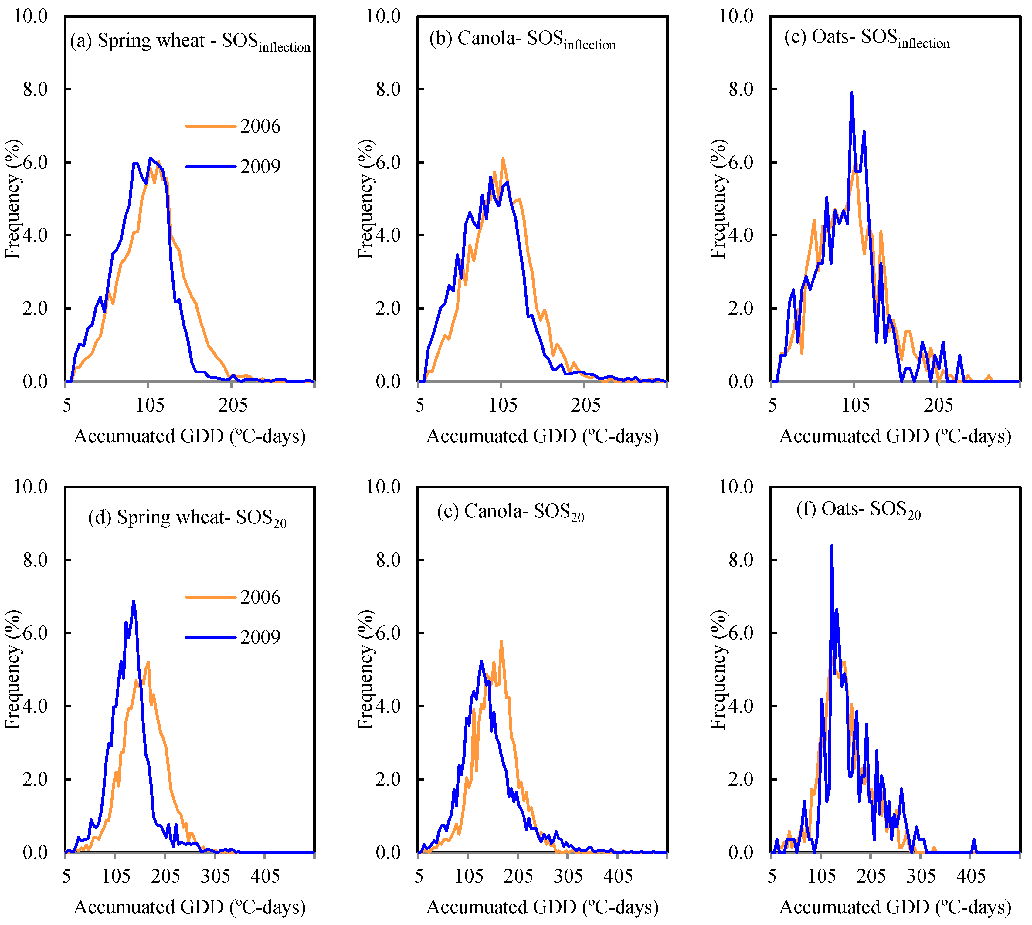
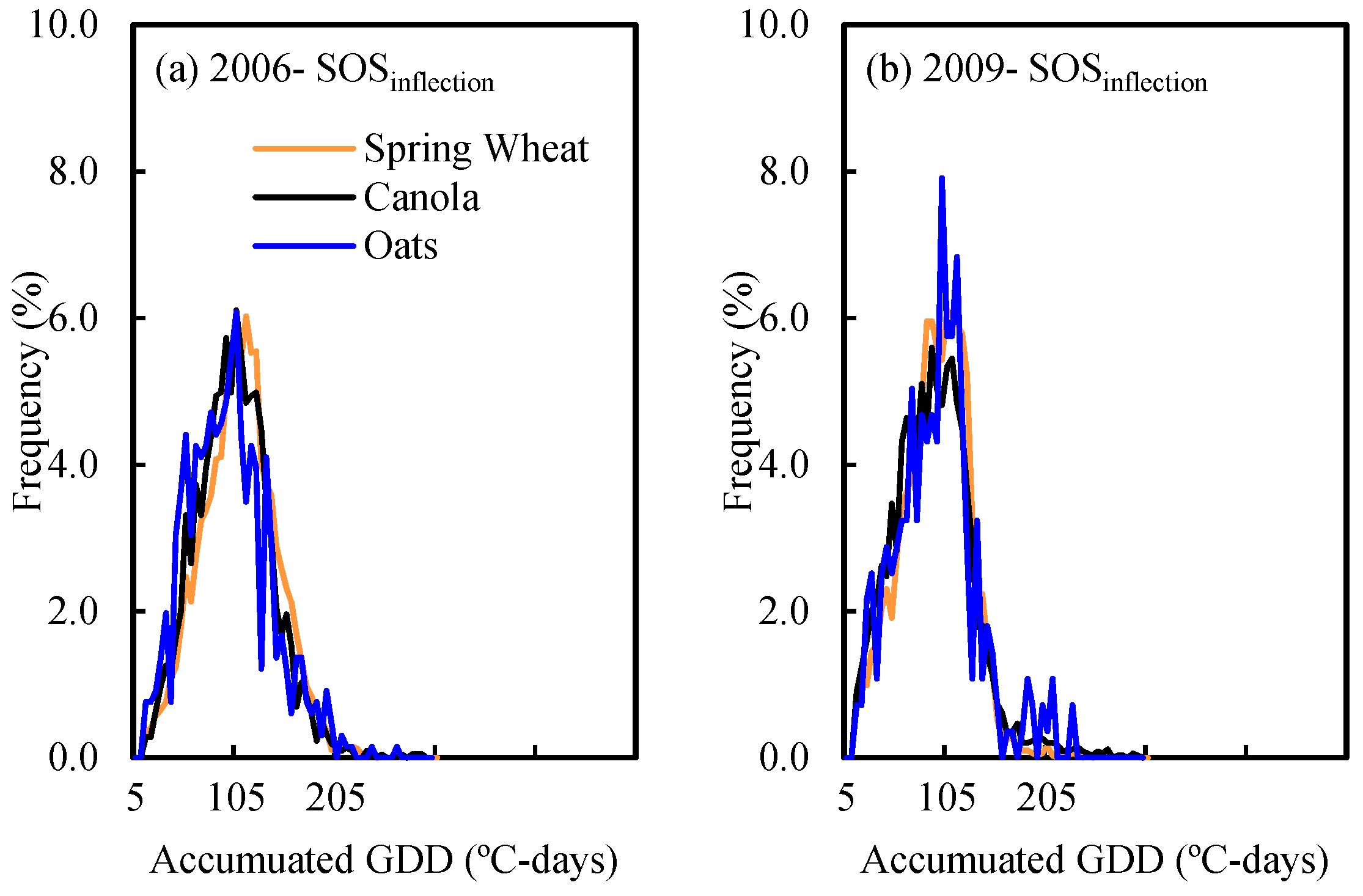
3.1. Statistical Characteristics of Observed Seeding Date and Estimated SOS

Table 1. Statistical analysis of the observed seeding date and estimated Start-Of-Season; µ and σ are the mean and the standard deviation of the samples, respectively; DOY is the day of year.

Year	Crop Types	Sample Number	Seeding Date (DOY)		SOS20 (DOY)		SOSinflection (DOY)
			Range	µ ± σ	Range	µ ± σ	Range	µ ± σ
2006	Spring wheat	3918	110–166	132 ± 8.1	130–175	151 ± 5.8	117–171	145 ± 5.9
	Canola	2205	112–164	137 ± 7.3	137–178	154 ± 5.1	125–173	148 ± 5.3
	Oats	700	110–168	132 ± 9.7	124–169	149 ± 6.6	119–163	143 ± 6.7
2009	Spring wheat	3130	117–172	139 ± 10.1	146–194	162 ± 5.8	135–189	156 ± 5.9
	Canola	3696	119–172	147 ± 8.5	139–196	167 ± 5.7	125–185	160 ± 6.1
	Oats	288	125–171	147 ± 11.7	153–196	168 ± 8.0	141–191	160 ± 8.4

shows the summary statistics of the observed seeding date and the estimated SOS using the two approaches for the selected quarter sections and crops. The seeding window generally ranged from DOY (day of year) 110 to 175. In a same year, the difference of the average seeding date among the three crops was not large. Crops were seeded later in 2009 than in 2006 by one to two weeks. For SOS estimated using the two methods, the variability among the three crops and between the two years are similar to that of the observed seeding date. The standard deviation for the two remotely sensed SOS indictors for different crops and years was generally around 6 days, which is close to that of the observed seeding date. This suggests that inter-field variability of the remotely sensed SOS is in parallel with that of seeding date. The SOS_inflection was smaller (closer to the seeding date) than the SOS₂₀.

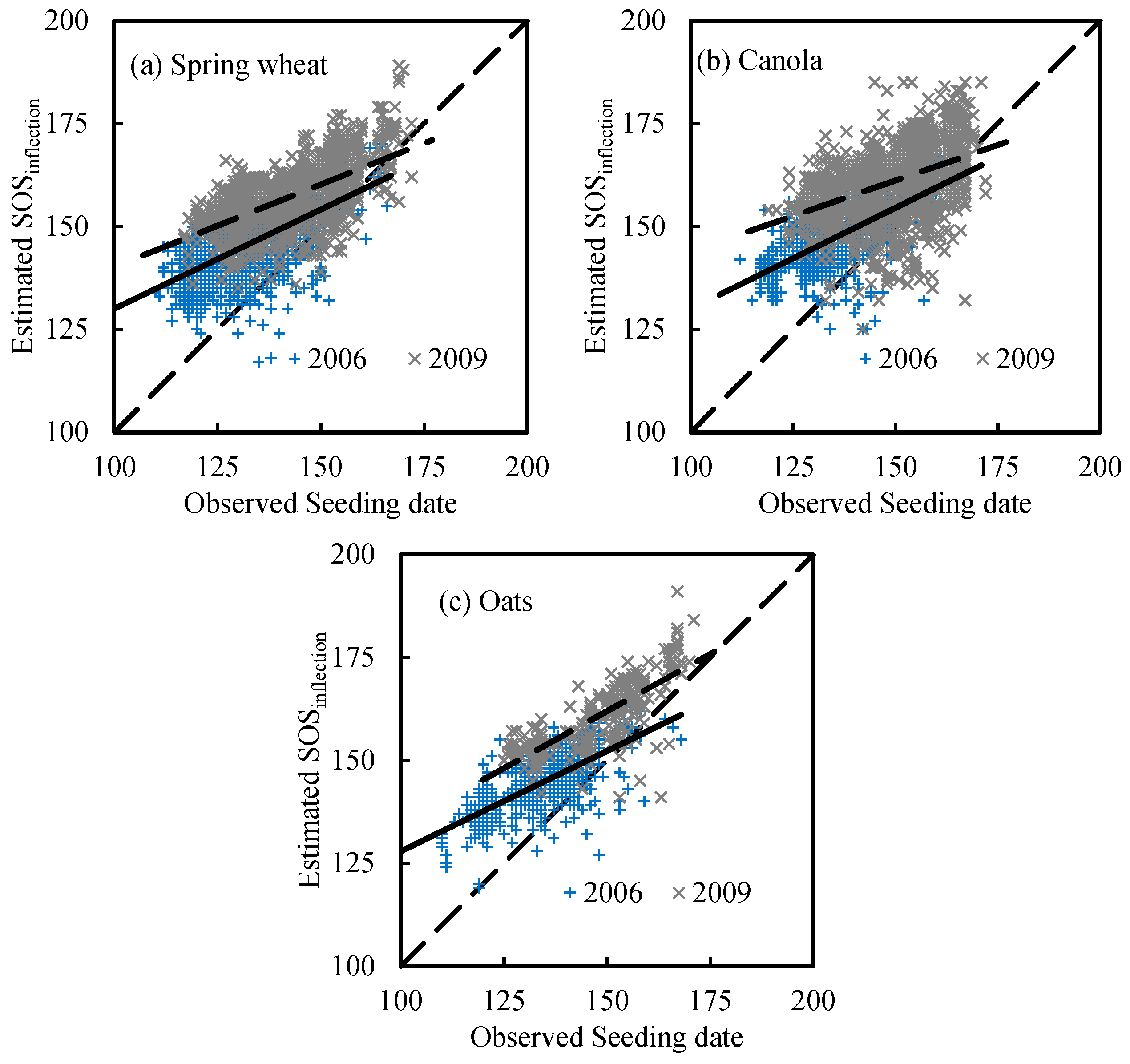
3.2. Relationships between Observed Seeding Date and SOS

For both 2006 and 2009 (Figure 3 and

Table 2. Linear regression between observed seeding date (x-axis) and Start-Of-Season (SOS; y-axis); R², RMSD (days) and Bias (days) are the coefficient of determination, the root-mean-square -difference, and the bias, respectively. Both RMSD and Bias are derived from the difference between observed seeding date and SOS.

Linear Regression Model		Crops	Regression	R2	RMSD (days)	Bias (days)
2006	SOSinflection	Spring Wheat	y = 0.48x + 81.82	0.44	14.9	13.6
		Canola	y = 0.49x + 80.87	0.46	12.0	9.9
		Oats	y = 0.49x + 79.15	0.50	13.2	11.3
		All crops	y = 0.49x + 80.15	0.48	13.9	12.2
	SOS20	Spring wheat	y = 0.51x + 84.46	0.51	20.2	19.4
		Canola	y = 0.50x + 85.48	0.50	17.1	15.4
		Oats	y = 0.54x + 78.84	0.61	18.4	17.4
		All crops	y = 0.51x + 83.83	0.55	19.1	17.9
2009	SOSinflection	Spring wheat	y = 0.40x + 100.18	0.47	17.9	16.3
		Canola	y = 0.34x + 109.50	0.19	15.0	12.6
		Oats	y = 0.56x + 78.65	0.60	15.1	13.1
		All crops	y = 0.41x + 99.49	0.38	16.4	14.3
	SOS20	Spring wheat	y = 0.44x + 101.76	0.58	24.0	23.0
		Canola	y = 0.39x + 110.37	0.27	21.0	19.6
		Oats	y = 0.58x + 82.57	0.73	21.7	20.7
		All crops	y = 0.45x + 100.94	0.48	22.4	21.1

), the observed seeding dates correlate well with the remotely sensed SOS derived using the two methods (SOS₂₀ and the SOS_inflection). The linear correlation between the seeding date and SOS₂₀ was generally stronger than that between the seeding date and the SOS_inflection. The slopes of the regression lines between the seeding date and remotely sensed SOS for both years were generally smaller than 1.0 with a positive bias, indicating that the earlier the seeding date, the longer the gap between seeding date and remotely sensed SOS. This is reasonable because air temperature normally increases during the seeding time in spring, hence the number of days needed for seed to accumulate enough AGDD to emerge decreases with time (Figure 2). As the inflection point used for SOS_inflection extraction is much closer to the point at the 10% of vegetation growth amplitude [15], the slopes of the regression lines between the seeding date and SOS₂₀ were generally higher than that between the seeding date and SOS_inflection. The RMSD between SOS₂₀ and the observed seeding date was generally around 20 days, while the RMSD between the SOS_inflection and the observed seeding date was about 14 days (Table 2). Based on the Chow test [54], the difference of linear regression between 2006 and 2009 for each crop is significant (p< 0.001), indicating that relationship between seeding date and remotely sensed SOS is year-specific.

Within the same year, the linear relationship between observed seeding date and SOS for the three crops was similar, and the RMSD between SOS and the observed seeding date was generally similar (Figure 4 and Table 2). Coefficients for the linear regression (the regression and intercept coefficient) among the three crops was small, and a general linear regression for the three crops can be developed. However, for inter-annual comparison, the RMSD was generally larger in 2009 than in 2006. SOS_inflection and the observed seeding date was about 23 days in 2009 and 19 days in 2006, showing a better correlation between seeding date and SOS in 2006 (Figure 2). The linear regression of each crop was different in different years (Figure 3); therefore, the seeding date of Manitoba in different years cannot be directly estimated from the remotely sensed SOS.

3.3. Accumulated Growing Degree Days

The cumulative GDD (AGDD) from the observed seeding date to remotely sensed SOS was calculated for each sample location. The histogram of both the AGDD_SOS for the SOS_inflection (AGDD_{SOS,inflection} ) and the SOS₂₀ (AGDD_SOS,20) were derived for each of the three selected crops (Figure 5 and

Table 3. Summary of the distribution of accumulative growing degree days (AGDD) from observed seeding date to remotely sensed SOS (AGDD_SOS) for different crops and years; µ and σ are the average value and the standard deviation value of AGDD_SOS, respectively.

Year.	Crops	AGDDSOS, 20 (°C-days)		AGDDSOS, inflection (°C-days)
		µ ± σ	95% Confidence Intervals	µ ± σ	95% Confidence Intervals
2006	Spring wheat	158.1 ± 42.7	74.4–241.8	106.0 ± 37.3	32.8–179.1
	Canola	156.1 ± 43.0	71.8–240.4	100.1 ± 37.1	27.5–172.8
	Oats	147.0 ± 47.6	53.7–240.3	95.0 ± 40.7	15.3–174.6
	All crops	156.3 ± 43.4	71.2–241.5	103.0 ± 37.8	28.9–177.0
2009	Spring wheat	130.2 ± 41.6	48.7–211.7	91.3 ± 33.9	24.8–157.9
	Canola	142.3 ± 55.9	32.7–252.0	89.5 ± 40.9	9.3–170.0
	Oats	159.7 ± 55.3	51.2–268.1	93.4 ± 43.2	8.7–178.2
	All crops	137.6 ± 50.6	38.4–236.9	90.5 ± 38.1	15.9–165.1

). The AGDD_sos for different crops and years follow a normal distribution. The AGDD_{SOS,inflection} was in general smaller than the AGDD_SOS,20 by about 50 °C-days (Table 3), which means that SOS_inflection was earlier than SOS₂₀. Based on the two years under study, crop growth required about 95 °C-days from seeding date to SOS_inflection (AGDD_{SOS,inflection}), and 150 °C–days from seeding date to SOS₂₀ (AGDD_SOS,20) (Table 3). The results in Figure 5 also show that the distributions of AGDD_SOS (AGDD_SOS,20 or AGDD_{SOS,inflection}) for the same crop type are different between the two years, however, the differences were relatively small. There are about 10 °C-days difference for the average value of AGDD_SOS,20 or AGDD_{SOS,inflection} (Table 3). This suggests that AGDD_SOS might be treated as non-year-specific. More importantly, AGDD_SOS within a year was not different for different crops (Figure 6). For instance, the mean and standard deviation value of AGDD_SOS,₂₀ in 2006 for each crop are around 150 °C-days and 43 °C-days, respectively (Table 3). Unlike the linear regression between seeding date and remotely sensed SOS, the AGDD_SOS was more uniform among crops and years. The results also reveal that the values of both AGDD_SOS,20 and AGDD_{SOS,inflection} are relatively stable between the two years with different weather conditions. Therefore, a general AGDD_SOS window (Table 3) can be determined for seeding-date estimation of different years and crops from remotely sensed SOS.

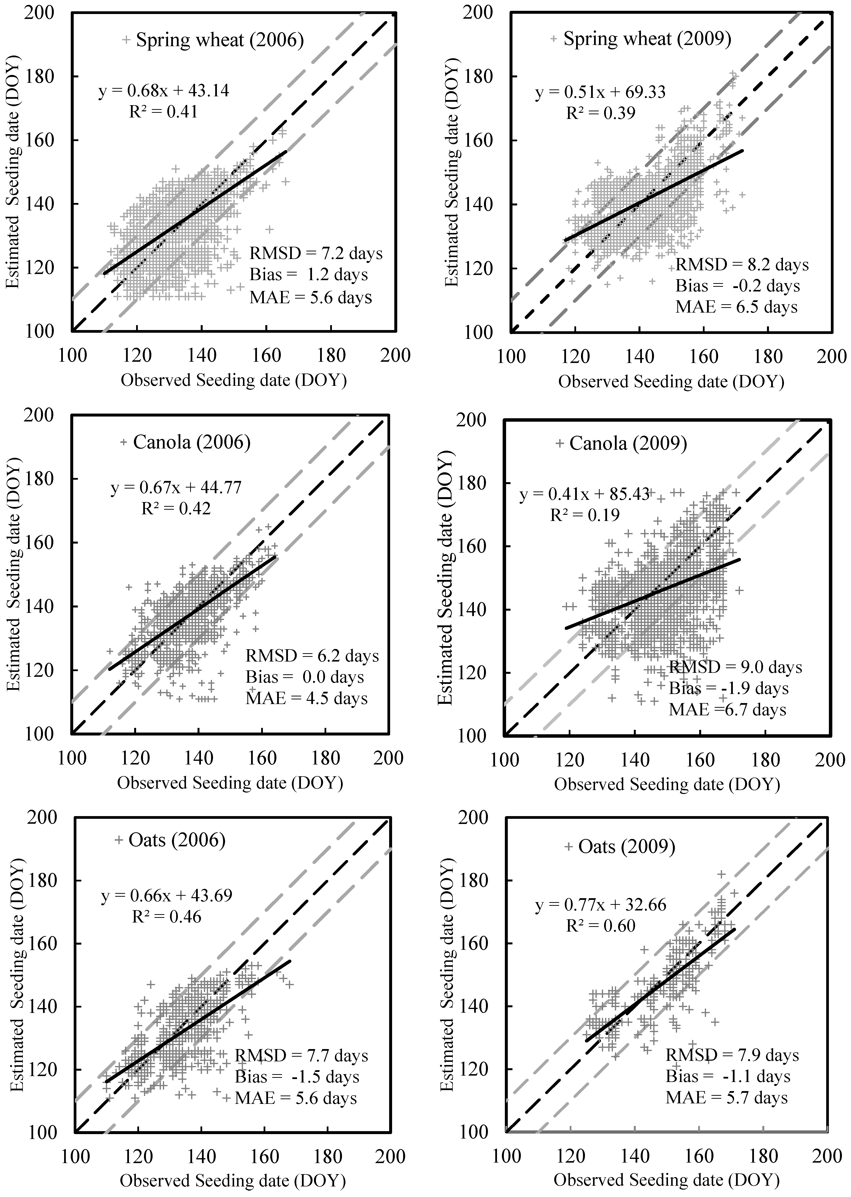
3.4. Accuracy of Estimated Seeding Date

Based on the AGDD_SOS window, the estimated seeding dates in both 2006 and 2009 using either the SOS₂₀ or SOS_inflection show good agreement with the observed seeding dates (Figure 7 and Figure 8). The statistical criteria (R², RMSD, bias and MAE) for evaluating the performance are also given in

Table 4. Accuracy assessment of the estimated seeding date from remotely sensed SOS using R², RMSD, bias and Mean Absolute Error (MAE).

Model		Crops	Overall
			R2	RMSD (days)	Bias	MAE (days)
2006	SOSinflection	Spring wheat	0.41	7.2	1.2	5.6
		Canola	0.42	6.2	0.0	4.5
		Oats	0.46	7.7	-1.5	5.6
		All crops	0.46	6.9	0.6	5.3
	SOS20	Spring wheat	0.50	7.4	1.3	5.9
		Canola	0.43	6.9	0.9	5.2
		Oats	0.59	7.5	-0.8	5.8
		All crops	0.52	7.3	1.0	5.7
2009	SOSinflection	Spring wheat	0.39	8.2	-0.2	6.5
		Canola	0.19	9.0	-1.9	6.7
		Oats	0.60	7.9	-1.1	5.7
		All crops	0.36	8.7	-0.8	6.6
	SOS20	Spring wheat	0.54	7.4	-0.1	5.8
		Canola	0.34	9.0	-0.8	7.0
		Oats	0.71	8.2	2.1	6.5
		All crops	0.50	8.3	-0.4	6.5

. The samples are generally distributed along the 1:1 line. The RMSD values are generally less than 10 days, and the bias mostly ranges from -2 to 2 days (Table 4). More importantly, there are no large differences in the errors for different crops and years. For instance, the RMSD of seeding date estimation using SOS₂₀ for the three crops was around 7.0 days in 2006, and 8.0 days in 2009. Using SOS₂₀, the RMSD and the MAE of the estimated seeding date of spring wheat were 7.4 and 5.9 days in 2006, and 7.4 and 5.8 in 2009, respectively. The performances of the two methods (inflection and threshold) were comparable. Similar results were also observed for canola and oats. These results suggest that a general range of AGDD for the SOS₂₀ or SOS_inflection (Table 3), independent of crop types and years, can be made. Thus, it is anticipated that the proposed model (Equations (4) and (5)) using AGDD_SOS,₂₀ or AGDD_{SOS, inflection} is generic, and crop seeding date can be accurately estimated for other years without model re-parameterization.

Table 4 also reveals that the overall accuracy of estimated seeding date using SOS_inflection is comparable with that of using SOS₂₀, as assessed using RMSD. However, the amount of variability in seeding date accounted for by SOS₂₀ was generally larger than that using SOS_inflection, as reflected by R² (Table 4). The slope of the linear regression between observed and estimated seeding date using SOS₂₀ was closer to 1.0 compared with that using SOS_inflection (Figure 7 and Figure 8). Thus, the estimated seeding date using SOS₂₀ is considered better for characterizing the temporal and spatial variability of seeding date in Manitoba than that of using SOS_inflection.

4. Discussion

4.1. Benefit of the Proposed Method

This study proposed a method for improved estimation of crop seeding date by incorporating remotely sensed SOS and GDD using two years’ of test data collected in Manitoba, Canada. Firstly, the study examined the dynamic ranges of AGDD between crop seeding date and the remotely sensed SOS (SOS₂₀ and SOS_inflection) for three crops, spring wheat, canola and oats. The estimated AGDD_SOS (base 5 °C) for canola was within the range reported by Miller et al. [22] and the North Dakota Agricultural Weather Network for canola growth in North American (https://ndawn.ndsu.nodak.edu/). The estimated AGDD for the SOS_inflection (AGDD_{SOS,inflection,} around 100 °C-days, base 5 °C) corresponds to the AGDD (< 142 °C-days, base 5 °C) required from crop seeding to crop emergence, and the estimated AGDD for the SOS₂₀ (AGDD_SOS,20, around 150 °C-days, base 5 °C) corresponds to the AGDD from seeding date to the stage with two/three leaves unfolded (143–220 °C-days, base 5 °C). For spring wheat, AGDD_SOS,20 around 150 °C-days (base 5 °C) is consistent with the AGDD (base 5 °C) observation from seeding date to the 2.5 Haun stage (two fully extended leaves and half of fully extended for the third leaf) in western Canada that was reported by Mkhabela et al. [32]. This suggests that the derived phenological metric SOS from remote sensing is physically related to a specific development stage of a crop.

The study also confirmed that the AGDD_SOS of a specific crop is relatively stable among years [27,29,35]. This is different from the number of days between the observed seeding date and remotely sensed SOS which vary with years because of varying weather conditions (Table 2 and Figure 3). Hence, reparametrizing the regression between the observed seeding date and remotely sensed SOS is often required if the crop seeding date is to be estimated using remotely sensed SOS alone. The seeding date of the three crops was not substantially different in 2006 or 2009 (Table 1), and the profiles of EVI2 time series during the vegetative stage were close to each other for the three crops (Figure 9). This resulted in small differences of estimated SOS among the three crops within a year (Table 2). By incorporating the AGDD_SOS to account for climate variation from year to year, a model can be established to estimate crop seeding date from remotely sensed SOS without the need for model recalibration.

Using the method developed in this study, error of the estimated seeding date was generally below 10 days, as evaluated using the RMSD (Table 4). Our study provides an improved estimation of seeding date compared with studies in the literature [8,13,18,21]. For instance, Manfron et al. [8] developed a rule-based approach to estimate seeding date of winter wheat in Camargue, France, using 250-m MODIS EVI product and obtained an estimated accuracy of RMSD = 22.05 days and MAE = 16.5 days. In contrast to many studies reported in the literature [7,13,21], we conducted the estimation and evaluation of seeding date at field level. The proposed method in our study could be extended to other crops and to other regions in Canada. This method could be used for seeding date estimation before the reproductive phases as SOS can be well extracted from time-series remotely sensed observations (e.g., VIs and biophysical variables) acquired before the reproductive phase [11,50].

4.2. Limitations of the Study

Given the promising results of this study, there is still room for improvement. For instance, the uncertainties in remotely sensed SOS extraction can lead to errors in seeding date estimation, as remotely sensed SOS could not be accurately estimated if time series EVI2 is considerably contaminated by noise and cannot be well reconstructed in some cases [47,55,56]. This is largely due to the quality of the EVI2 observations and the selected mathematical functions for curve fitting. In particular, Manitoba has a long winter season, and snow cover may have strong influence on parameter optimization of the selected mathematical functions, especially the minimum EVI2 [57,58,59]. The threshold-based method depends highly on the accuracies of the reconstructed maximum and minimum EVI2. However, the peak EVI2 of a growing season cannot be accurately estimated as retrieving the optimal parameters of the mathematical function (e.g., logistic and PDHT function) is highly dependent on the quality and number of the EVI2 observations [58]. Shang et al. [15] reported that remotely sensed SOS cannot be accurately extracted using the inflection-based method if the profile of the EVI2 time series does not follow a logistic function well. This is also true for the PDHT function. This would be the main reason that very small or large gaps between seeding date and remotely sensed SOS existed in some of the samples (Figure 3). According to the study by Chen et al. [55], the PDHT function or the logistic function integrated with other reconstruction approaches, such as the locally adjusted cubic-spline capping (LACC) [55] and the adaptive local iterative logistic fitting method [50], might help in reducing the error of the remotely sensed SOS. Developing an approach to retrieve VI corresponding to bare soil (minimum VI) from historical VI records [57,58], or improving a VI to be resistant to the influence of snow cover (e.g., Normalized Difference Phenology Index (NDPI) [60]) will also improve the extraction of SOS and other phenological metrics in the study area. Furthermore, harmonizing multi-sources data, such as fusing MODIS with other high spatial optical data (e.g., Sentinel-2) and SAR data (e.g., Sentinel-1 and RADARSAT-2) [61,62,63], is likely to improve the quality of phenology extraction and seeding date estimation, particularly for the heterogeneous area with mixed crops.

In addition to air temperature, other factors such as soil moisture, soil temperature, seeding rate and seeding depth can also impact crop emergence [23,64]. In this study, only air temperature was considered; taking into consideration of other factors in the estimation process could further improve the accuracy of seeding date estimation from remote sensing data.

The proposed method was evaluated based on the two years of data with different climatic variability. However, more data are required to evaluate the stability of the model for different years, locations and crops.

5. Conclusions

In this study, a method was developed for crop seeding-date estimation, and the results were evaluated using data collected in 2006 and 2009 in Manitoba, Canada. The method uses GDD to convert SOS derived from time-series MODIS data to crop seeding date. The test results show that the seeding dates of three major crops (spring wheat, canola, and oats) could be accurately estimated at the field level. On average, the estimation error based on RMSD was within 10 days of observed values.

The study also revealed that the linear regression between the observed seeding date and remotely sensed SOS varies with years. Subtracting a constant number of days from the remotely sensed SOS to estimate crop seeding date over large areas and across different years could therefore result in large errors. By integrating the calibrated AGDD_SOS, seeding date could be better estimated from SOS for different crops in different years. We observed that SOS derived using a threshold-based approach (SOS₂₀) was more stable and accurate for seeding date estimation than SOS derived using an approach (SOS_inflection) based on the inflection point of a vegetation index curve. The SOS₂₀ is therefore recommended for seeding date estimation over large areas and different years. It is anticipated that this method can be adapted to other crops at other locations using the same or different satellite data.

In future studies, the method will be further evaluated among different crops in the Canadian Prairies. Time-series of seeding date for different crops based on historical remote sensing data (e.g. AVHRR and MODIS) will be derived for assessing the crop production in response to climate change. In addition, other information (e.g., soil moisture and soil temperature) derived from multi-source remote sensing data (e.g., Sentinel-1 and RADARSAT-2) will be considered to further improve the stability of the proposed model, and data assimilation will be incorporated in seeding-date estimation.

References

1. Araya, A.; Stroosnijder, L.; Habtu, S.; Keesstra, S.D.; Berhe, M.; Hadgu, K.M. Risk assessment by sowing date for barley (hordeum vulgare) in northern ethiopia. Argic. For. Meterol. 2012, 154–155, 30–37. [Google Scholar] [CrossRef]
2. May, W.E.; Mohr, R.M.; Lafond, G.P.; Johnston, A.M.; Stevenson, F.C. Early seeding dates improve oat yield and quality in the eastern prairies. Can. J. Plan. Sci. 2004, 84, 431–442. [Google Scholar] [CrossRef]
3. Sacks, W.J.; Deryng, D.; Foley, J.A.; Ramankutty, N. Crop planting dates: An analysis of global patterns. Globa. Ecol. Biogeo. 2010, 19, 607–620. [Google Scholar] [CrossRef]
4. Soler, C.M.T.; Sentelhas, P.C.; Hoogenboom, G. Application of the csm-ceres-maize model for planting date evaluation and yield forecasting for maize grown off-season in a subtropical environment. Euro. J. Agron. 2007, 27, 165–177. [Google Scholar] [CrossRef]
5. Chang, K.-H.; Warland, J.S.; Bartlett, P.A.; Arain, A.M.; Yuan, F. A simple crop phenology algorithm in the land surface model cn-class. Agron. J. 2014, 106, 297–308. [Google Scholar] [CrossRef]
6. Dobor, L.; Barcza, Z.; Hlásny, T.; Árendás, T.; Spitkó, T.; Fodor, N. Crop planting date matters: Estimation methods and effect on future yields. Argic. For. Meterol. 2016, 223, 103–115. [Google Scholar] [CrossRef]
7. Urban, D.; Guan, K.; Jain, M. Estimating sowing dates from satellite data over the U.S. Midwest: A comparison of multiple sensors and metrics. Remote Sens. Environ. 2018, 211, 400–412. [Google Scholar] [CrossRef]
8. Manfron, G.; Delmotte, S.; Busetto, L.; Hossard, L.; Ranghetti, L.; Brivio, P.A.; Boschetti, M. Estimating inter-annual variability in winter wheat sowing dates from satellite time series in camargue, france. Int. J. App. Earth Obs. Geoinf. 2017, 57, 190–201. [Google Scholar] [CrossRef]
9. Canisius, F.; Shang, J.; Liu, J.; Huang, X.; Ma, B.; Jiao, X.; Geng, X.; Kovacs, J.M.; Walters, D. Tracking crop phenological development using multi-temporal polarimetric radarsat-2 data. Remote Sens. Environ. 2018, 210, 508–518. [Google Scholar] [CrossRef]
10. Song, C.; Chen, J.M.; Hwang, T.; Gonsamo, A.; Croft, H.; Zhang, Q.; Dannenberg, M.; Zhang, Y.; Hakkenberg, C.; Li, J. Ecological characterization of vegetation using multisensor remote sensing in the solar reflective spectrum. Land Res. Monitor. Model. Map. Remote Sens. 2015, 2, 533–575. [Google Scholar]
11. Zhang, X.; Friedl, M.A.; Schaaf, C.B.; Strahler, A.H.; Hodges, J.C.; Gao, F.; Reed, B.C.; Huete, A. Monitoring vegetation phenology using modis. Remote Sens. Environ. 2003, 84, 471–475. [Google Scholar] [CrossRef]
12. Marinho, E.; Vancutsem, C.; Fasbender, D.; Kayitakire, F.; Pini, G.; Pekel, J.-F. From remotely sensed vegetation onset to sowing dates: Aggregating pixel-level detections into village-level sowing probabilities. Remote Sens. 2014, 6, 10947–10965. [Google Scholar] [CrossRef]
13. Lobell, D.B.; Ortiz-Monasterio, J.I.; Sibley, A.M.; Sohu, V.S. Satellite detection of earlier wheat sowing in india and implications for yield trends. Agric. Sys. 2013, 115, 137–143. [Google Scholar] [CrossRef]
14. Liu, L.; Zhang, X.; Yu, Y.; Guo, W. Real-time and short-term predictions of spring phenology in north america from viirs data. Remote Sens. Environ. 2017, 194, 89–99. [Google Scholar] [CrossRef]
15. Shang, R.; Liu, R.; Xu, M.; Liu, Y.; Zuo, L.; Ge, Q. The relationship between threshold-based and inflexion-based approaches for extraction of land surface phenology. Remote Sens. Environ. 2017, 199, 167–170. [Google Scholar] [CrossRef]
16. Ren, J.; Campbell, J.B.; Shao, Y. Estimation of sos and eos for midwestern us corn and soybean crops. Remote Sens. 2017, 9. [Google Scholar] [CrossRef]
17. Sakamoto, T.; Wardlow, B.D.; Gitelson, A.A.; Verma, S.B.; Suyker, A.E.; Arkebauer, T.J. A two-step filtering approach for detecting maize and soybean phenology with time-series modis data. Remote Sens. Environ. 2010, 114, 2146–2159. [Google Scholar] [CrossRef]
18. Kotsuki, S.; Tanaka, K. Sacra – a method for the estimation of global high-resolution crop calendars from a satellite-sensed ndvi. Hydrol. Earth Syst. Sci. 2015, 19, 4441–4461. [Google Scholar] [CrossRef]
19. Zeng, L.; Wardlow, B.D.; Wang, R.; Shan, J.; Tadesse, T.; Hayes, M.J.; Li, D. A hybrid approach for detecting corn and soybean phenology with time-series modis data. Remote Sens. Environ. 2016, 181, 237–250. [Google Scholar] [CrossRef]
20. Duchemin, B.; Fieuzal, R.; Rivera, M.A.; Ezzahar, J.; Jarlan, L.; Rodriguez, J.C.; Hagolle, O.; Watts, C. Impact of sowing date on yield and water use efficiency of wheat analyzed through spatial modeling and formosat-2 images. Remote Sens. 2015, 7, 5951–5979. [Google Scholar] [CrossRef]
21. Vyas, S.; Nigam, R.; Patel, N.; Panigrahy, S. Extracting regional pattern of wheat sowing dates using multispectral and high temporal observations from indian geostationary satellite. J. India. Soc. Remote Sens. 2013, 41, 855–864. [Google Scholar] [CrossRef]
22. Miller, P.; Lanier, W.; Brandt, S. Using growing degree days to predict plant stages; Montana State University-Bozeman: Bozeman, MO, USA, 2001. [Google Scholar]
23. Wang, E.; Engel, T. Simulation of phenological development of wheat crops. Agric. Sys. 1998, 58, 1–24. [Google Scholar] [CrossRef]
24. Sacks, W.J.; Kucharik, C.J. Crop management and phenology trends in the us corn belt: Impacts on yields, evapotranspiration and energy balance. Argic. For. Meterol. 2011, 151, 882–894. [Google Scholar] [CrossRef]
25. Anandhi, A. Growing degree days – ecosystem indicator for changing diurnal temperatures and their impact on corn growth stages in kansas. Ecolog. Indica. 2016, 61, 149–158. [Google Scholar] [CrossRef]
26. Ortiz-Monasterio, J.I.; Lobell, D.B. Remote sensing assessment of regional yield losses due to sub-optimal planting dates and fallow period weed management. Field Crop. Res. 2007, 101, 80–87. [Google Scholar] [CrossRef]
27. Akyuz, F.A.; Kandel, H.; Morlock, D. Developing a growing degree day model for north dakota and northern minnesota soybean. Argic. For. Meterol. 2017, 239, 134–140. [Google Scholar] [CrossRef]
28. Forcella, F.; Benech Arnold, R.L.; Sanchez, R.; Ghersa, C.M. Modeling seedling emergence. Field Crop. Res. 2000, 67, 123–139. [Google Scholar] [CrossRef]
29. McMaster, G.S.; Wilhelm, W. Growing degree-days: One equation, two interpretations. Argic. For. Meterol. 1997, 87, 291–300. [Google Scholar] [CrossRef]
30. Qian, B.; De Jong, R.; Warren, R.; Chipanshi, A.; Hill, H. Statistical spring wheat yield forecasting for the canadian prairie provinces. Argic. For. Meterol. 2009, 149, 1022–1031. [Google Scholar] [CrossRef]
31. Saiyed, I.M.; Bullock, P.R.; Sapirstein, H.D.; Finlay, G.J.; Jarvis, C.K. Thermal time models for estimating wheat phenological development and weather-based relationships to wheat quality. Can. J. Plant Sci. 2009, 89, 429–439. [Google Scholar] [CrossRef]
32. Mkhabela, M.; Ash, G.; Grenier, M.; Bullock, P. Testing the suitability of thermal time models for forecasting spring wheat phenological development in western canada. Can. J. Plant Sci. 2016, 96, 765–775. [Google Scholar] [CrossRef]
33. Waha, K.; Van Bussel, L.; Müller, C.; Bondeau, A. Climate-driven simulation of global crop sowing dates. Glob. Ecol. Biogeogr. 2012, 21, 247–259. [Google Scholar] [CrossRef]
34. Srivastava, A.K.; Mboh, C.M.; Gaiser, T.; Webber, H.; Ewert, F. Effect of sowing date distributions on simulation of maize yields at regional scale – a case study in central ghana, west africa. Agric. Syst. 2016, 147, 10–23. [Google Scholar] [CrossRef]
35. Skakun, S.; Franch, B.; Vermote, E.; Roger, J.-C.; Becker-Reshef, I.; Justice, C.; Kussul, N. Early season large-area winter crop mapping using modis ndvi data, growing degree days information and a gaussian mixture model. Remote Sens. Environ. 2017, 195, 244–258. [Google Scholar] [CrossRef]
36. Zhong, L.; Gong, P.; Biging, G.S. Efficient corn and soybean mapping with temporal extendability: A multi-year experiment using landsat imagery. Remote Sens. Environ. 2014, 140, 1–13. [Google Scholar] [CrossRef]
37. Franch, B.; Vermote, E.F.; Becker-Reshef, I.; Claverie, M.; Huang, J.; Zhang, J.; Justice, C.; Sobrino, J.A. Improving the timeliness of winter wheat production forecast in the united states of america, ukraine and china using modis data and ncar growing degree day information. Remote Sens. Environ. 2015, 161, 131–148. [Google Scholar] [CrossRef]
38. Soil Classification Working Group. The canadian system of soil classification. Agric. Agri-Food Canada Publ. 1998, 187. Available online: https://www.nrcresearchpress.com/doi/abs/10.1139/9780660174044#.XTqkLXERXIU (accessed on 15 July 2019).
39. Armstrong, R.N.; Pomeroy, J.W.; Martz, L.W. Variability in evaporation across the canadian prairie region during drought and non-drought periods. J. Hydrol. 2015, 521, 182–195. [Google Scholar] [CrossRef]
40. Thornton, P.E.; Thornton, M.M.; Mayer, B.W.; Wei, Y.; Devarakonda, R.; Vose, R.S.; Cook., R.B. Daymet: Daily Surface Weather Data on a 1-km Grid for North America, Version 3; ORNL DAAC: Oak Ridge, TN, USA, 2017.
41. Shang, J.; Liu, J.; Ma, B.; Zhao, T.; Jiao, X.; Geng, X.; Huffman, T.; Kovacs, J.M.; Walters, D. Mapping spatial variability of crop growth conditions using rapideye data in Northern Ontario, Canada. Remote Sens. Environ. 2015, 168, 113–125. [Google Scholar] [CrossRef]
42. Dong, T.; Liu, J.; Shang, J.; Qian, B.; Ma, B.; Kovacs, J.M.; Walters, D.; Jiao, X.; Geng, X.; Shi, Y. Assessment of red-edge vegetation indices for crop leaf area index estimation. Remote Sens. Environ. 2019, 222, 133–143. [Google Scholar] [CrossRef]
43. Jiang, Z.; Huete, A.R.; Didan, K.; Miura, T. Development of a two-band enhanced vegetation index without a blue band. Remote Sens. Environ. 2008, 112, 3833–3845. [Google Scholar] [CrossRef]
44. Zhang, X.; Wang, J.; Gao, F.; Liu, Y.; Schaaf, C.; Friedl, M.; Yu, Y.; Jayavelu, S.; Gray, J.; Liu, L. Exploration of scaling effects on coarse resolution land surface phenology. Remote Sens. Environ. 2017, 190, 318–330. [Google Scholar] [CrossRef] [Green Version]
45. Dong, T.; Liu, J.; Shang, J.; Qian, B.; Huffman, T.; Zhang, Y.; Champagne, C.; Daneshfar, B. Assessing the impact of climate variability on cropland productivity in the canadian prairies using time series modis fapar. Remote Sens. 2016, 8. [Google Scholar] [CrossRef]
46. Markwardt, C.B. Non-linear least squares fitting in idl with mpfit. arXiv 2009, arXiv:0902.2850. [Google Scholar]
47. de Beurs, K.M.; Henebry, G.M. Spatio-temporal statistical methods for modelling land surface phenology. In Phenological Research; Springer: Dordrecht, the Netherlands, 2010; pp. 177–208. [Google Scholar]
48. You, X.; Meng, J.; Zhang, M.; Dong, T. Remote sensing based detection of crop phenology for agricultural zones in china using a new threshold method. Remote Sens. 2013, 5. [Google Scholar] [CrossRef]
49. White, M.A.; Thornton, P.E.; Running, S.W. A continental phenology model for monitoring vegetation responses to interannual climatic variability. Glob. Biogeochem. Cycles 1997, 11, 217–234. [Google Scholar] [CrossRef]
50. Cao, R.; Chen, J.; Shen, M.; Tang, Y. An improved logistic method for detecting spring vegetation phenology in grasslands from modis evi time-series data. Argic. For. Meterol. 2015, 200, 9–20. [Google Scholar] [CrossRef]
51. Yang, Y.; Wilson, L.T.; Wang, J. A spatially explicit crop planting initiation and progression model for the conterminous united states. European J. Agron. 2017, 90, 184–197. [Google Scholar] [CrossRef]
52. Duveiller, G.; Lopez-Lozano, R.; Cescatti, A. Exploiting the multi-angularity of the modis temporal signal to identify spatially homogeneous vegetation cover: A demonstration for agricultural monitoring applications. Remote Sens. Environ. 2015, 166, 61–77. [Google Scholar] [CrossRef]
53. Dwyer, L.M.; Hayhoe, H.N.; Culley, J.L.B. Prediction of soil temperature from air temperature for estimating corn emergence. Can. J. Plant Sci. 1990, 70, 619–628. [Google Scholar] [CrossRef]
54. Chow, G.C. Tests of equality between sets of coefficients in two linear regressions. Econo. J. Econ. Soc. 1960, 591–605. [Google Scholar] [CrossRef]
55. Chen, J.M.; Deng, F.; Chen, M. Locally adjusted cubic-spline capping for reconstructing seasonal trajectories of a satellite-derived surface parameter. IEEE Trans. Geosci. Remote Sens. 2006, 44, 2230–2238. [Google Scholar] [CrossRef]
56. Jönsson, P.; Eklundh, L. Timesat. A program for analyzing time-series of satellite sensor data. Com. Geosci. 2004, 30, 833–845. [Google Scholar] [CrossRef]
57. Beck, P.S.A.; Atzberger, C.; Høgda, K.A.; Johansen, B.; Skidmore, A.K. Improved monitoring of vegetation dynamics at very high latitudes: A new method using modis ndvi. Remote Sens. Environ. 2006, 100, 321–334. [Google Scholar] [CrossRef]
58. Liu, R. Compositing the minimum ndvi for modis data. IEEE Trans. Geosci. Remote Sens. 2017, 55, 1396–1406. [Google Scholar] [CrossRef]
59. Studer, S.; Stöckli, R.; Appenzeller, C.; Vidale, P.L. A comparative study of satellite and ground-based phenology. Int. J. Bimetero. 2007, 51, 405–414. [Google Scholar] [CrossRef] [PubMed]
60. Wang, C.; Chen, J.; Wu, J.; Tang, Y.; Shi, P.; Black, T.A.; Zhu, K. A snow-free vegetation index for improved monitoring of vegetation spring green-up date in deciduous ecosystems. Remote Sens. Environ. 2017, 196, 1–12. [Google Scholar] [CrossRef]
61. Liao, C.; Wang, J.; Dong, T.; Shang, J.; Liu, J.; Song, Y. Using spatio-temporal fusion of landsat-8 and modis data to derive phenology, biomass and yield estimates for corn and soybean. Sci. Total. Environ. 2019, 650, 1707–1721. [Google Scholar] [CrossRef]
62. Dong, T.; Liu, J.; Qian, B.; Zhao, T.; Jing, Q.; Geng, X.; Wang, J.; Huffman, T.; Shang, J. Estimating winter wheat biomass by assimilating leaf area index derived from fusion of landsat-8 and modis data. Int. J. App. Earth Obs. Geoinfor. 2016, 49, 63–74. [Google Scholar] [CrossRef]
63. Veloso, A.; Mermoz, S.; Bouvet, A.; Le Toan, T.; Planells, M.; Dejoux, J.-F.; Ceschia, E. Understanding the temporal behavior of crops using sentinel-1 and sentinel-2-like data for agricultural applications. Remote Sens. Environ. 2017, 199, 415–426. [Google Scholar] [CrossRef]
64. Chakraborty, A.; Sesha Sai, M.V.R.; Murthy, C.S.; Roy, P.S.; Behera, G. Assessment of area favourable for crop sowing using amsr-e derived soil moisture index (amsr-e smi). Int. J. App. Earth Obs. Geoinfor. 2012, 18, 537–547. [Google Scholar] [CrossRef]
Figure 1. The study area in the Province of Manitoba, Canada, and the distribution of annual cropland in 2009. The subset figure highlights the location of the study area within Canada.
Remotesensing 11 01760 g001
Figure 2. Variability of daily mean temperature (a) and accumulated growing degree days (AGDD, °C-days, base 5 °C) (b) for the years 2006 and 2009.
Remotesensing 11 01760 g002
Figure 3. Scatter plot of observed seeding date and remotely sensed Start-Of-Season (SOS) for spring wheat (a,d), canola (b,e), and oats (c,f) in 2006 and 2009; DOY is the day of year. The dashed black, the long dashed black and the solid black line denote the 1:1 line, the linear regression between observed seeding date and SOS in 2006 and 2009, respectively.
Remotesensing 11 01760 g003aRemotesensing 11 01760 g003b
Figure 4. Scatter plot of observed seeding date and remotely sensed SOS for different years: 2006 (a,c) and 2009 (b,d); DOY is the day of year, and the dashed black line denotes the 1:1 lines.
Remotesensing 11 01760 g004
Figure 5. Histogram of AGDD from seeding date to the remotely sensed SOS using the inflection-based (SOSinflection) and the threshold-based method (SOS20) for spring wheat (a,d), canola (b,e), and oats (c,f) in 2006 and 2009, respectively.
Remotesensing 11 01760 g005
Figure 6. Histogram of AGDD from seeding date to the remotely sensed SOS using the inflection-based (SOSinflection) and that using the threshold-based method (SOS20) for 2006 (a,c) and 2009 (b,d), respectively.
Remotesensing 11 01760 g006aRemotesensing 11 01760 g006b
Figure 7. Comparison between observed and estimated seeding date using the inflection based approach (SOSinflection); the dashed gray lines mark is the 10-day confidence interval, and the dashed black line denotes the 1:1 lines.
Remotesensing 11 01760 g007
Figure 8. Comparison between observed and estimated seeding date using the threshold based approach (SOS20); the dashed gray lines mark the 10-day confidence interval, and the dashed black line denotes the 1:1 line.
Remotesensing 11 01760 g008
Figure 9. Time-series EVI2 for the three crops (spring wheat, canola and oats) in two different years (2006 (a) and 2009 (b)). The two grey vertical lines highlight the period of vegetative stage.
Remotesensing 11 01760 g009