Estimating Forest Leaf Area Index and Canopy Chlorophyll Content with Sentinel-2: An Evaluation of Two Hybrid Retrieval Algorithms

Abstract

Estimates of biophysical and biochemical variables such as leaf area index (LAI) and canopy chlorophyll content (CCC) are a fundamental requirement for effectively monitoring and managing forest environments. With its red-edge bands and high spatial resolution, the Multispectral Instrument (MSI) on board the Sentinel-2 missions is particularly well-suited to LAI and CCC retrieval. Using field data collected throughout the growing season at a deciduous broadleaf forest site in Southern England, we evaluated the performance of two hybrid retrieval algorithms for estimating LAI and CCC from MSI data: the Scattering by Arbitrarily Inclined Leaves (SAIL)-based L2B retrieval algorithm made available to users in the Sentinel Application Platform (SNAP), and an alternative retrieval algorithm optimised for forest environments, trained using the Invertible Forest Reflectance Model (INFORM). Moderate performance was associated with the SNAP L2B retrieval algorithm for both LAI (r² = 0.54, RMSE = 1.55, NRMSE = 43%) and CCC (r² = 0.52, RMSE = 0.79 g m⁻², NRMSE = 45%), while improvements were obtained using the INFORM-based retrieval algorithm, particularly in the case of LAI (r² = 0.79, RMSE = 0.47, NRMSE = 13%), but also in the case of CCC (r² = 0.69, RMSE = 0.52 g m⁻², NRMSE = 29%). Forward modelling experiments confirmed INFORM was better able to reproduce observed MSI spectra than SAIL. Based on our results, for forest-related applications using MSI data, we recommend users seek retrieval algorithms optimised for forest environments.

1. Introduction

Estimates of biophysical and biochemical variables such as leaf area index (LAI) and canopy chlorophyll content (CCC) provide vital information on the condition, structure and function of vegetation canopies. They are a key input into climate and numerical weather prediction models, and characterising their spatial and temporal dynamics is crucial in understanding biogeochemical fluxes between the biosphere and atmosphere [1,2,3]. Of particular importance for modelling terrestrial carbon exchange are forest environments, which cover approximately 30% of the terrestrial surface and account for approximately 50% of its gross primary productivity [4,5]. In addition to carbon sequestration, forests provide a range of ecosystem services, acting as a source of food, fibre, fuel and timber [6]. If we are to effectively monitor and manage these resources, estimates of the biophysical and biochemical variables that describe their status are a fundamental requirement.

Estimating LAI and CCC in the field is a time-consuming and labour-intensive process that is often constrained by logistical challenges and financial resources. Advances in indirect, non-destructive field-based techniques have provided increases in efficiency [7,8,9], but nevertheless, field observations are insufficient to characterise spatial and temporal variability in LAI and CCC at regional to global scales. Satellite remote sensing data are particularly advantageous in this respect, offering consistent, repeat observations with global coverage. Over the last two decades, methods of retrieving vegetation biophysical and biochemical variables from optical satellite remote sensing have been established, typically making use of radiative transfer models (RTMs) that simulate canopy reflectance as a function of biophysical and biochemical properties [10,11,12].

Retrieval approaches that have proven popular for generating operational products include the inversion of RTMs using look-up-tables (LUTs) [13,14], in addition to hybrid methods, which use RTM outputs to train machine learning algorithms such as artificial neural networks (ANNs) [15,16,17]. When compared to LUT inversion, hybrid methods are typically more computationally efficient [10,18,19,20]. This is because large LUTs are required to achieve high retrieval accuracies, slowing inversion, which involves searching the LUT on a per-pixel basis [10,11,21]. In contrast, hybrid methods such as ANNs are able to accurately represent complex non-linear relationships, and provide an input to output mapping that can be applied almost instantly [21,22,23]. Thus, they can be quickly and automatically applied to large data sets, while providing comparable retrieval accuracies [12,18,19]. The principle drawbacks of ANNs are their ‘black box’ nature, the need to specify and tune the network architecture, and their tendency to perform unpredictably when inputs strongly deviate from their training data [10,20].

With its red-edge bands and high spatial resolution (10 m to 60 m), the Multispectral Instrument (MSI) on-board the Sentinel-2 missions is well-suited to vegetation biophysical and biochemical variable retrieval [24]. In particular, its spectral sampling opens up opportunities for the retrieval of CCC, to which the position of the red-edge is highly sensitive [25,26,27,28,29]. A considerable body of work related to the retrieval of vegetation biophysical and biochemical variables using MSI data has been published in recent years, although the majority of studies have been restricted to agricultural environments containing crop canopies. Despite the importance of forest environments, few studies have focussed on forest biophysical and biochemical variable retrieval from MSI data [28,30,31,32]. Of these, the majority have relied on simulated MSI data that cannot fully represent the observational characteristics of the instrument in orbit (i.e., they make use of resampled airborne, field spectroradiometer or RTM data, with different viewing/illumination geometries and atmospheric characteristics).

Although estimates of LAI and CCC are not produced operationally by the Sentinel-2 ground segment, a retrieval algorithm is provided in the freely available Sentinel Application Platform (SNAP), enabling users to generate so-called ‘L2B’ products. Developed by Weiss and Baret [33], the algorithm is based on the hybrid retrieval approach, making use of a series of ANNs. Each is pre-trained using the coupled Scattering by Arbitrarily Inclined Leaves (SAIL) and Leaf Optical Properties Spectra (PROSPECT) RTMs [34,35]. While the SNAP L2B retrieval algorithm is described as generic, providing reasonable retrieval accuracies over all vegetation types [33], previous work has demonstrated poor performance when RTMs such as SAIL, which describe the canopy as a turbid medium, are applied over forest environments [23]. Because of its ease of use and integration within the image processing software, it is expected that many users will adopt the SNAP L2B retrieval algorithm as a first port of call. Although good performance has been demonstrated over crop canopies [36,37,38,39], evaluation of its performance over forest canopies would enable users to more explicitly assess its fitness for purpose for non-agricultural applications, particularly when compared to retrieval algorithms specifically optimised for forest environments.

Using data collected throughout the first full year of the Sentinel-2 mission during a series of field campaigns, we assess the performance of the SNAP L2B retrieval algorithm for estimating LAI and CCC over a deciduous broadleaf forest site in Southern England. We also develop and evaluate an alternative hybrid retrieval algorithm optimised for forest environments, trained using the Invertible Forest Reflectance Model (INFORM) [40]. The objectives of the paper are to:

• Determine the retrieval accuracy that can be expected when the SNAP L2B retrieval algorithm (which is based on SAIL and not optimised for forest environments) is used for LAI and CCC retrieval over deciduous broadleaf forest.
• Evaluate the extent to which a retrieval algorithm trained using INFORM (and thus optimised for forest environments) will improve LAI and CCC retrieval accuracy.

2. Materials and Methods

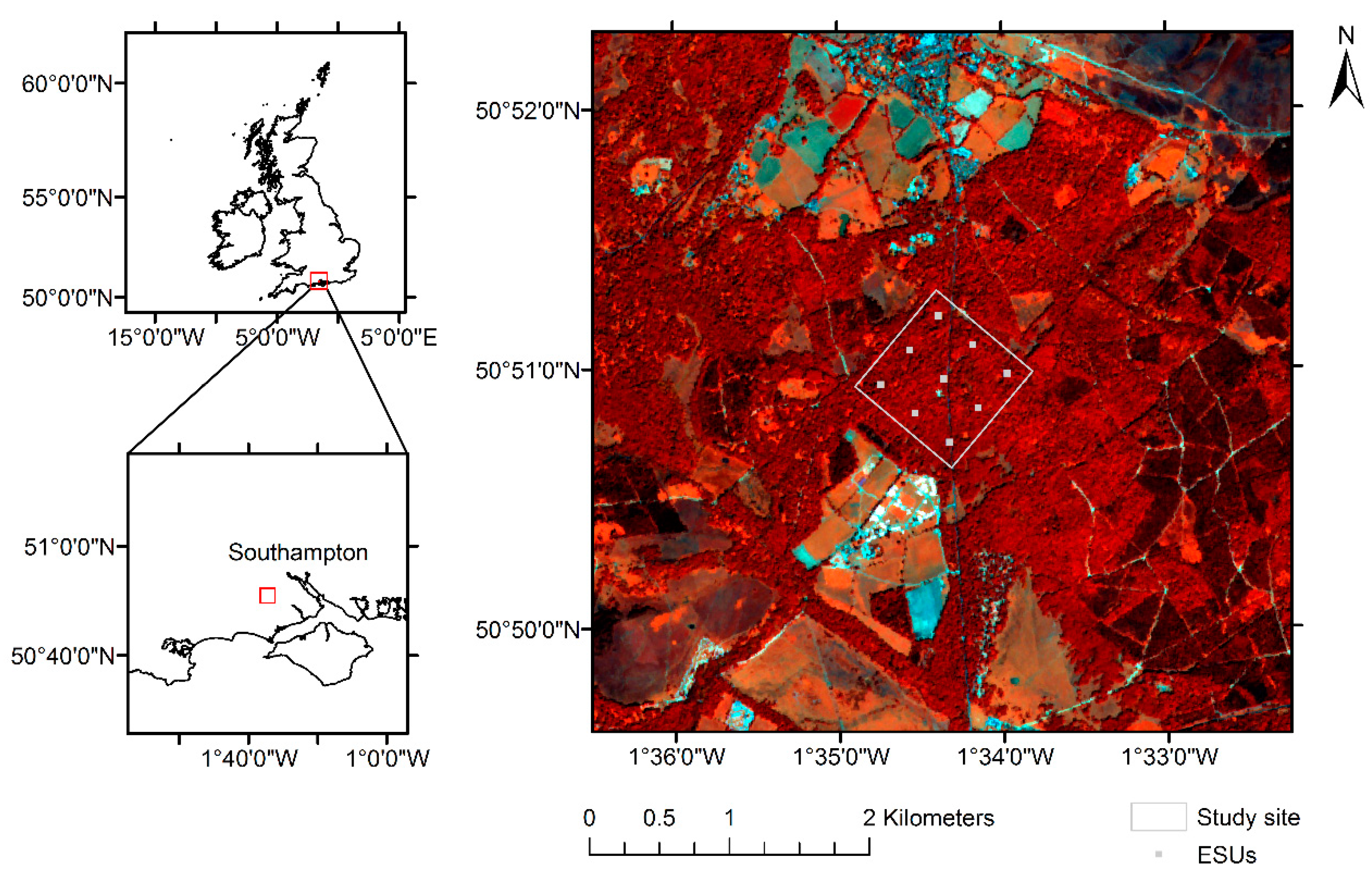
2.1. Study Site

The study site (50.8498°N, 1.5741°W) covers a 1 km × 1 km area in the New Forest National Park, Hampshire, United Kingdom, and is comprised of deciduous broadleaf forest (Figure 1). Lying approximately 40 m above sea level, the site is a unique example of ancient and ornamental woodland, dating back to the 17th century. The dominant species are beech (Fagus sylvatica) (45%), oak (Quercus robur) (40%) and silver birch (Betula pendula) (5%), while the dominant soil type is a dark-grey clay loam. Statistics of key stand attributes are listed in

Table 1. Statistics of key stand attributes after Cantarello and Newton [43] and Mountford et al. [44].

Stand Attribute	Minimum	Maximum	Mean	Standard Deviation
Canopy height (m)	10	34	-	-
Diameter at breast height (cm)	25.9	80.5	43.4	12.9
Crown diameter (m)	5.76	14.29	8.49	3.73
Stem density (ha−1)	72	536	256	106

. The site has previously been used in the validation of a range of satellite-derived vegetation biophysical and biochemical variables [41,42].

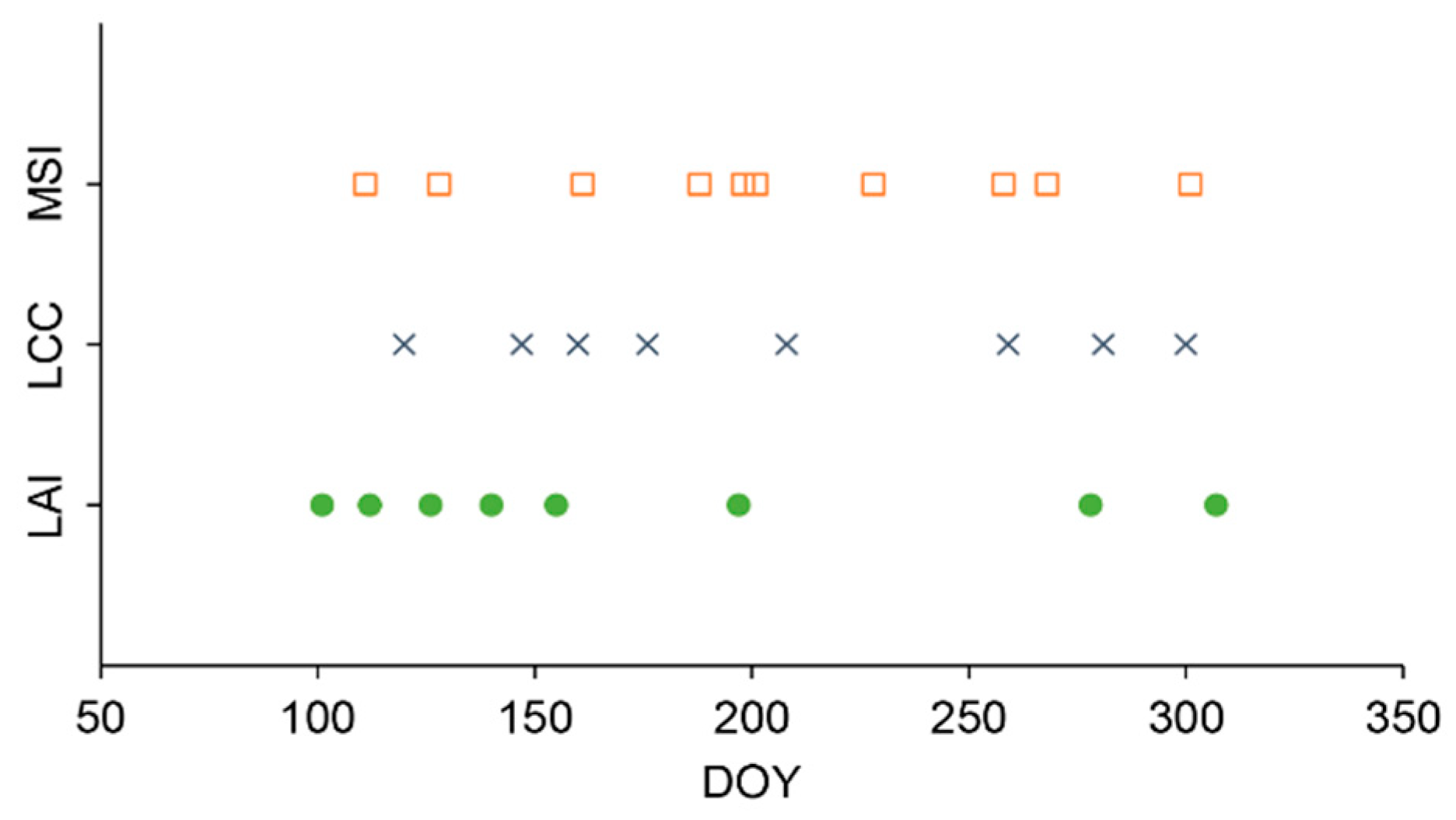
2.2. Field Data Collection and Processing

Field data were collected on sixteen dates throughout 2016, enabling the phenological cycle to be captured between day of year (DOY) 101 and 307 (Figure 2). A total of nine ESUs of 40 m × 40 m were established over the study site in a regular grid pattern, enabling spatial variability in LAI and CCC to be characterised (Figure 1). All nine ESUs were sampled on each measurement date. The ESU dimensions were selected according to Justice and Townshend [45], to enable the known 10 m positional uncertainty in the investigated 20 m MSI data to be accounted for [46]. The location of each ESU was determined using a handheld Garmin eTrex H global positioning system (GPS) device, which has a reported positional error of less than 10 m [47]. Within each ESU, sampling was carried out at five points arranged in a cross pattern, following the approach adopted in the BigFoot project [48]. The four peripheral points were located approximately 20 m from the central point. Despite the fact that several species are present in the forest, all selected ESUs were dominated by a single species.

Leaf area index (LAI) was derived using digital hemispherical photography (DHP). Images were acquired using a Nikon Coolpix 4500 digital camera equipped with an FC-E8 fisheye lens, calibrated using the procedures described by Weiss and Baret [49]. To calculate LAI from each image, pixels were first classified as belonging to the vegetation canopy or its background, enabling the gap fraction to be calculated. Each image was then divided into ten zenith rings of 7.5°, and each zenith ring further divided into 48 azimuth cells of 7.5°. Only zenith angles of less than 75° were considered to minimise the influence of mixed pixels at the extremes of the image [8,49]. Finally, LAI was derived as a discretisation of Miller’s [50] integral, such that

$$LAI=2{\displaystyle \sum }_{i=1}^{10}-\overline{\ln P\left({\theta }_i\right)}\cos {\theta }_i\sin {\theta }_i\mathrm{d}{\theta }_i$$

(1)

where $P\left({\theta }_i\right)$ is the gap fraction in ring $i$ and ${\theta }_i$ is its central zenith angle. The effects of foliage clumping were accounted for according to Lang and Yueqin [51] by calculating the mean of the natural logarithm of gap fraction values over all azimuth cells in each zenith ring. Please note that because the classification could not distinguish between foliage and other canopy elements, the resulting estimates also contained some contribution from other plant material such as stems and branches [7,8,52].

Canopy chlorophyll content (CCC) was calculated as the product of LAI and leaf chlorophyll concentration (LCC) in g m⁻². Estimates of LCC were typically obtained within several days of LAI measurements (Figure 2) using a Konica Minolta SPAD-502 optical chlorophyll meter, which determines a relative value proportional to LCC based on the ratio of incident and transmitted radiation at 650 nm and 940 nm. Relative values were converted to absolute units using species–specific calibration functions [53,54]. Three leaves were removed from the tree closest to each sampling point, and each tree was marked using coloured rope to enable re-identification during subsequent surveys. For each leaf, three replicates were performed to account for variations in LCC across its surface, yielding a total of nine measurements per sampling location, and 45 per ESU. Care was taken to avoid major veins within the leaf [9,54].

2.3. Interpolation of Field Data

When evaluating biophysical and biochemical variables derived from high spatial resolution instruments such as MSI, temporal scaling issues are of increased importance, particularly in areas of high cloud cover such as our study site. While spatial scaling issues have received considerable attention in the context of validating operational biophysical and biochemical products [55,56,57,58], approaches for dealing with the temporal mismatch between field and satellite observations are less mature [37]. Traditionally, field observations have been matched to the closest satellite acquisition, often within the bounds of an arbitrary period such as one week [59,60]. Such an approach assumes that there is little variation in vegetation condition within this period—an assumption that may be violated at the onset of greenness and senescence, during which rapid changes in biophysical and biochemical properties can occur.

In light of these issues, we adopted an interpolation-based approach that can be applied if field data are collected on multiple dates throughout the year. By interpolating multi-temporal field observations, variations in vegetation condition can better be accounted for, particularly if a parametric function is selected that encodes prior knowledge about expected vegetation dynamics. Importantly, the approach maximises the amount of cloud-free satellite data that can be used for comparison, while also enabling LAI and LCC data collected on different dates to be more easily integrated for the estimation of CCC. To facilitate interpolation, we fit double logistic functions to the LAI and LCC data collected at each ESU. The double logistic function is widely used to represent vegetation phenology [61,62,63], and takes the form

$$g\left(x\right)=a+\frac{b}{\left[1+\exp \left(c-dx\right)\right] \left[1+\exp \left(e-fx\right)\right]}$$

(2)

where $g\left(x\right)$ is the LAI or LCC value at a given DOY, $a$ is the base level, $b$ is the seasonal amplitude, $c$ and $d$ control the timing and rate of the onset of greenness, and $e$ and $f$ control the timing and rate of the onset of senescence. To assess their ability to accurately represent seasonal trajectories of the variables of interest throughout the study period, leave-one-out cross validation was carried out on double logistic functions fit to the mean values of LAI and LCC at each DOY. Each data point was sequentially removed before fitting, and its value predicted and compared to that observed. The absolute error was used to investigate the relative importance of each observation date, while overall accuracy was quantified using the root mean square error (RMSE).

2.4. MSI Data Pre-Processing

Ten L1C MSI products covering the growing season from DOY 111 to 300 were obtained over the study site and processed to L2A bottom-of-atmosphere (BOA) reflectance with Sen2Cor 2.5.5 [64], which performs atmospheric, cirrus, and terrain correction. It also provides a scene classification, in addition to estimates of aerosol optical thickness and water vapour. To restrict our analysis to high-quality, cloud-free data, pixels identified as cloud by the scene classification were discarded (three pixels from a total of 90).

2.5. Hybrid LAI and CCC Retrieval

From L2A BOA reflectance values, we first estimated LAI and CCC using the SNAP L2B retrieval algorithm as implemented in SNAP 6.0 [65]. In addition to cloud-contaminated pixels, retrievals flagged by the algorithm as having an out of range input or output were discarded (a further six pixels). Because the SNAP L2B retrieval algorithm is not optimised for forest environments, we also developed an alternative hybrid retrieval algorithm, trained using INFORM. As in the SNAP L2B retrieval algorithm, leaf reflectance spectra were simulated by PROSPECT. 50,000 simulations were carried out, in which input parameters were drawn randomly from a combination of fixed, uniform, and truncated Gaussian distributions (

Table 2. Distributions from which Invertible Forest Reflectance Model (INFORM) input parameters were randomly drawn.

Parameter	Minimum	Maximum	Mean	Standard Deviation	Distribution	Reference
Structural parameter (N)	1.5	1.7	-	-	Uniform	[72,73]
Chlorophyll a + b (µg cm−2)	10	60	50	20	Gaussian	This study
Dry matter (g cm−2)	0.004	0.02	-	-	Uniform	[72,73]
Equivalent water thickness (g cm−2)	0.01	0.02	-	-	Uniform	[72,73]
Average leaf angle (°)	55	55	-	-	Fixed	[72,73]
Single tree LAI	1.0	5.0	4.0	0.5	Gaussian	This study
Understory LAI	0.5	0.5	-	-	Fixed	[72,73]
Stem density (ha−1)	72	536	256	106	Gaussian	[43]
Canopy height (m)	10	34	-	-	Uniform	[44]
Crown diameter (m)	6	14	8	4	Gaussian	[43]
Solar zenith angle (°)	29	64	-	-	Uniform	This study
Observer zenith angle (°)	3	11	-	-	Uniform	This study
Relative azimuth angle (°)	20	136	-	-	Uniform	This study
Soil brightness coefficient	0.5	0.5	-	-	Fixed	[72]
Fraction of diffuse radiation	0.1	0.1	-	-	Fixed	[40,72,73]

). Retrieval algorithms trained with 50,000 simulations were shown to provide comparable retrieval accuracies to those utilising over 100,000 simulations by Weiss et al. [66], while additional simulations may not be beneficial in the case of machine learning algorithms such as ANNs, which are prone to overfitting [40,67]. It is worth noting that a similar number of simulations (41,472) was used by Weiss and Baret [33] to train the SNAP L2B retrieval algorithm. Soil background spectra were computed by selecting randomly from a spectral library containing 25 soils [68] and applying a multiplicative soil brightness coefficient (Table 2). INFORM output spectra were convolved with the MSI spectral response functions [69] to generate simulated reflectance values in MSI’s spectral bands.

To reflect uncertainties in the radiometric calibration and atmospheric correction of MSI data, simulated reflectance values were contaminated with wavelength-dependent and -independent Gaussian white noise [23]. This consisted of both additive (0.01) and multiplicative (2%) components [33,70,71], such that

$$R_{cont}\left(\mathsf{\lambda }\right)=R_{sim}\left(\mathsf{\lambda }\right) \left(1+\epsilon \left[0,{\sigma }_{multi}\left(\mathsf{\lambda }\right)\right]+\epsilon \left[0,{\sigma }_{multi}\left(all\right)\right]\right)+\epsilon \left[0,{\sigma }_{add}\left(\mathsf{\lambda }\right)\right]+\epsilon \left[0,{\sigma }_{add}\left(all\right)\right]$$

(3)

where $R_{cont}\left(\mathsf{\lambda }\right)$ and $R_{sim}\left(\mathsf{\lambda }\right)$ are the contaminated and simulated reflectance values in the band centered at $\mathsf{\lambda }$, $\epsilon \left[0,\sigma \right]$ is a Gaussian distribution with a mean of zero, while ${\sigma }_{add}\left(\mathsf{\lambda }\right)$, ${\sigma }_{multi}\left(\mathsf{\lambda }\right)$, ${\sigma }_{add}\left(all\right)$, and ${\sigma }_{multi}\left(all\right)$ are the additive and multiplicative components of wavelength dependent and independent Gaussian white noise respectively.

As in the SNAP L2B retrieval algorithm, an ANN-based retrieval approach was adopted. Each ANN was trained using the Levenberg-Marquardt minimisation algorithm, and comprised one hidden layer with five tangent sigmoid neurons, in addition to one output layer with a single linear neuron. Given sufficient training data, this architecture (which is also adopted by the SNAP L2B retrieval algorithm) has been found to perform as well as more complex ones [12,16,23,33]. A random subset of 50% of the simulations were used for training, while 25% were used for regularisation, and 25% were used for testing. To prevent overfitting, the regularisation subset was used to enable early stopping (i.e., training was halted when the error, as assessed using the regularisation subset, stopped continuing to decrease). The testing subset, which was not used in training or early stopping, was used to evaluate theoretical performance. Ten ANNs were trained, and the one with the best theoretical performance was selected for further analysis (Appendix A).

Because using a single ANN to estimate multiple biophysical variables can lead to comparatively poor performance [16,23], individual ANNs were trained to estimate LAI and CCC (as is also the case in the SNAP L2B retrieval algorithm). In addition to the simulated BOA reflectance in the eight MSI bands used by the SNAP L2B retrieval algorithm (

Table 3. MSI bands adopted by the SNAP L2B and INFORM-based retrieval algorithms.

Band	Central Wavelength (nm)	Bandwidth (nm)	Native Spatial Resolution (m)
B3	550	35	10
B4	665	30	10
B5	705	15	20
B6	740	15	20
B7	783	20	20
B8A	865	20	20
B11	1610	90	20
B12	2190	180	20

), ANN input variables included the cosine of the observer zenith angle (OZA), relative azimuth angle (RAA), and solar zenith angle (SZA), enabling variations in viewing and illumination geometry to be accounted for [21,33,70]. MSI band 2 was excluded because of the likelihood of residual atmospheric contamination [33]. All bands were resampled to a common spatial resolution of 20 m, in order to take advantage of MSI’s three red-edge bands (B5, B6 and B7).

2.6. Forward Modelling Experiments

A prerequisite to accurate biophysical and biochemical variable retrieval is that the underlying RTMs must be able to reproduce observed spectra in a satisfactory manner. To investigate the ability of SAIL and INFORM to reproduce observed MSI spectra over our study site, forward modelling experiments were carried out [74,75]. To simulate the MSI spectrum for each date and ESU, the interpolated field measurements of LAI and LCC were used in model parameterisation, as were the viewing and illumination geometries of the associated MSI scenes. Because the remaining input parameters were not measured in the field, they were instead randomly drawn from the distributions described in Section 2.5. For each date, ESU, and RTM, a database of 5,000 simulations was established. This number of simulations was considered appropriate given that nine input parameters were fixed, resulting in a substantially constrained parameter space. The reflectance mismatch was evaluated between the observed MSI spectrum and the best fitting simulation, which was itself determined as the simulation with the minimum RMSE [74,75].

2.7. Performance Metrics

To evaluate the performance of each retrieval algorithm, LAI and CCC retrievals were compared with values provided by the double logistic functions for the DOY in question. Agreement between the interpolated field data and LAI and CCC retrievals was assessed using the coefficient of determination (r²), while retrieval accuracy was quantified using the RMSE. A normalised RMSE (NRMSE) was calculated by dividing the RMSE by the mean of observed values. Bias was determined as the mean difference, while precision was quantified as the standard deviation of differences. In addition to calculating these statistics using all available data, statistics were also computed on three subsets to evaluate phenological variations in retrieval accuracy. These represented the onset of greenness (DOY 100 to 149), peak greenness (DOY 150 to 249), and the onset of senescence (DOY 250 to 300). The same performance metrics were adopted in the forward modelling experiments.

3. Results

3.1. Field Data and Interpolation

Throughout the study period, LAI ranged from a minimum of 0.81 on DOY 101 to a maximum of 4.60 on DOY 155, while LCC ranged from a minimum of 0.09 g m⁻² on DOY 120 to a maximum of 0.65 g m⁻² on DOY 259. It should be noted that the minimum LAI values corresponded mainly to stems and branches, which could not be distinguished from other canopy elements using DHP. At the start of the growing season, the rate of increase in LCC was slower than that of LAI (Figure 3). Unlike LCC observations, which became more variable towards the end of the growing season, the degree of variability associated with LAI observations remained relatively consistent between measurement dates (Figure 3). The double logistic functions fit to the field data were able to successfully represent seasonal trajectories of LAI and LCC throughout the study period (Figure 3). The results of leave-one-out cross validation revealed an RMSE of 0.10 for LAI and 0.11 g m⁻² for LCC. The largest absolute errors were observed when those observations during the onset of greenness and senescence were removed (

Table 4. Leave-one-out cross-validation results indicating the absolute error associated with interpolated LAI and LCC values on each sampling date (i.e., the error that would occur if that observation were not used in function fitting).

LAI		LCC
DOY	Absolute Error	DOY	Absolute Error (g m−2)
101	0.02	120	0.21
112	0.00	147	0.01
126	0.10	160	0.03
140	0.16	176	0.03
155	0.04	208	0.04
197	0.05	259	0.04
278	0.04	281	0.05
307	0.18	300	0.22

).

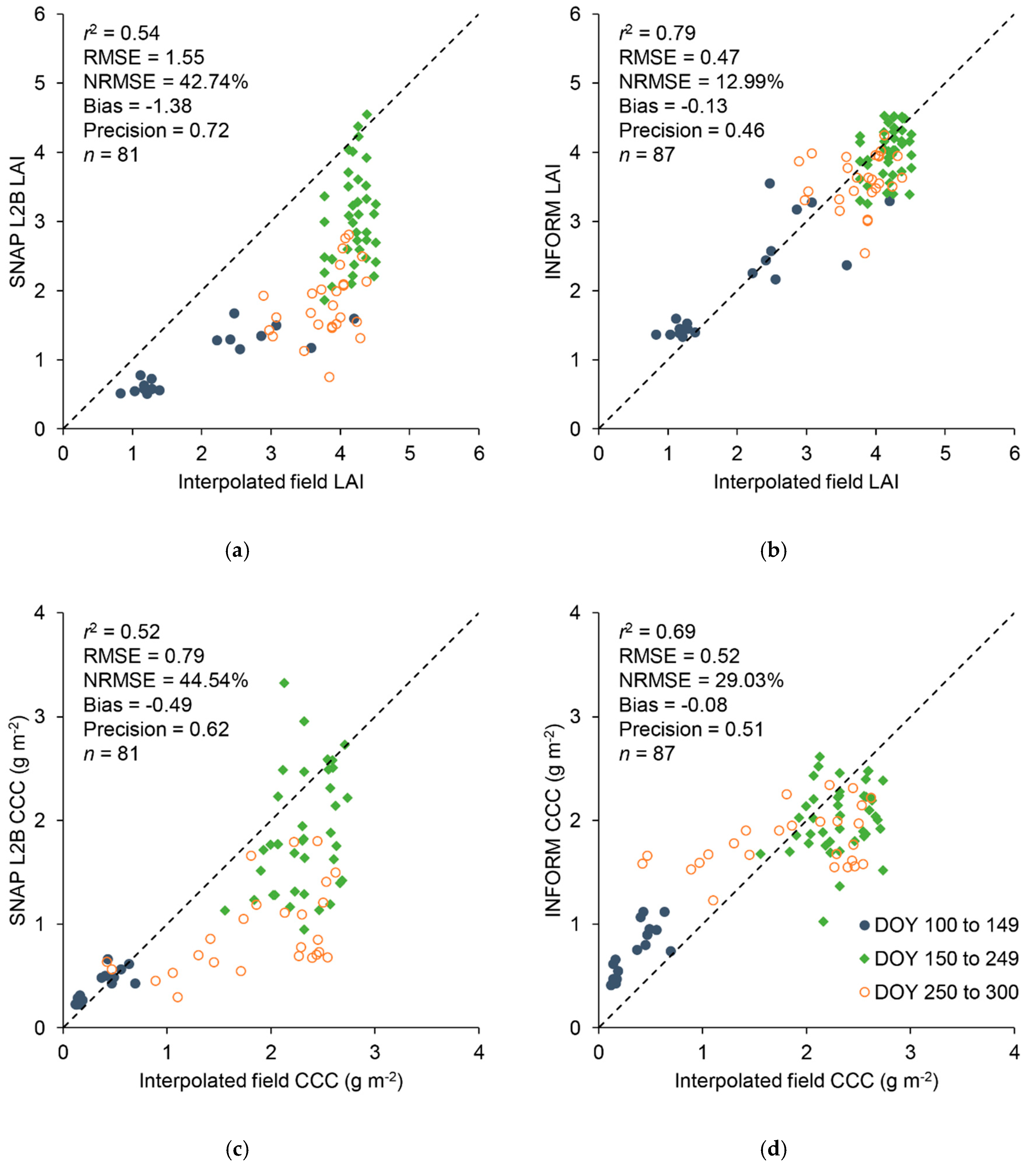
3.2. Overall Performance of the Retrieval Algorithms

Overall, the SNAP L2B retrieval algorithm was characterised by underestimation of LAI, leading to a moderate relationship and retrieval accuracy (r² = 0.54, RMSE = 1.55, NRMSE = 43%) (Figure 4a). Like LAI, SNAP L2B CCC retrievals were also characterised by a moderate relationship and retrieval accuracy (r² = 0.52, RMSE = 0.79 g m⁻², NRMSE = 45%) (Figure 4c). In contrast, a greater degree of consistency between the interpolated field data and INFORM-based LAI retrievals was observed, leading to a stronger relationship and increased retrieval accuracy (r² = 0.79, RMSE = 0.47, NRMSE = 13%) (Figure 4b). Improvements in overall performance were also evident for CCC (r² = 0.69, RMSE = 0.52, NRMSE = 29%) (Figure 4d).

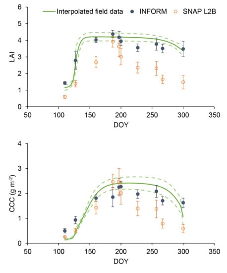
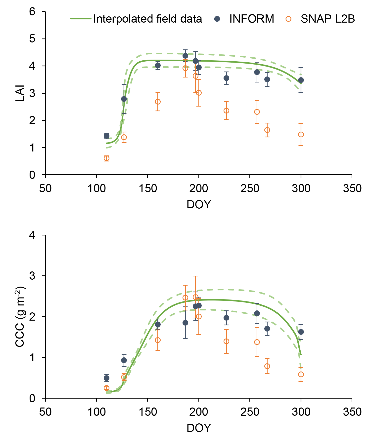
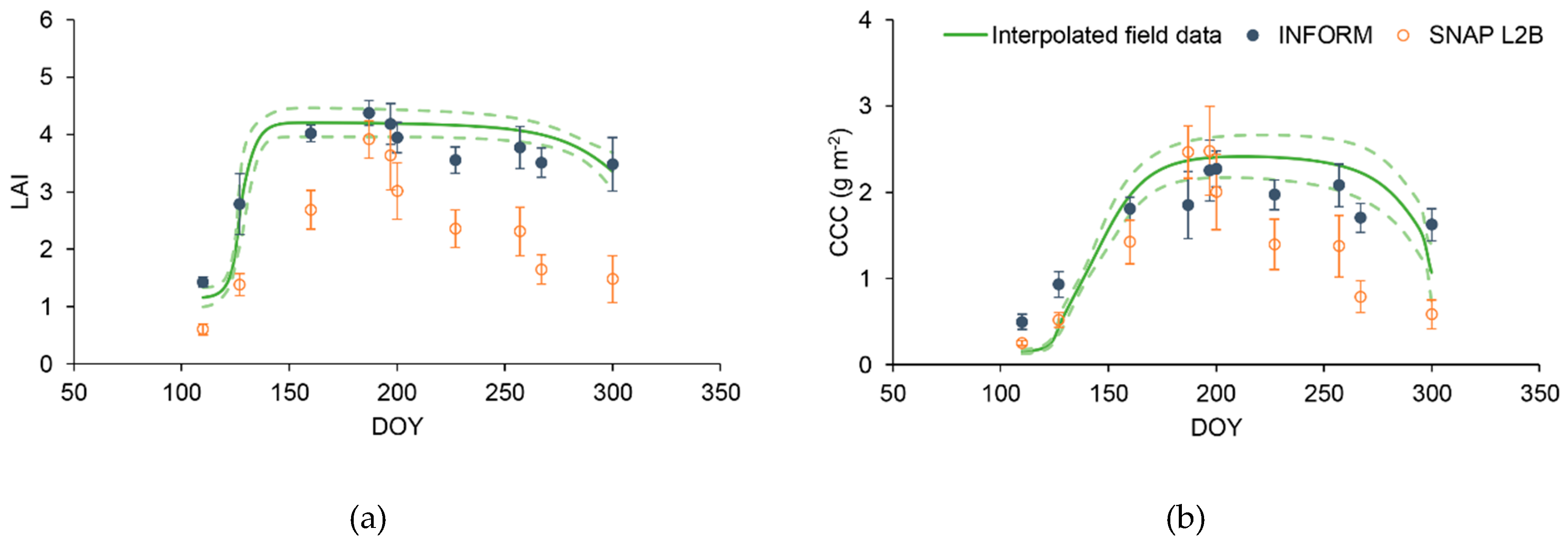
3.3. Phenological Variations in Performance

When the phenological subsets were examined, the strongest relationships with the interpolated field data were observed for the onset of greenness (DOY 100 to 149, r² = 0.66 to 0.77) (

Table 5. Performance statistics for the SNAP L2B and INFORM-based retrieval algorithms when evaluated against interpolated field data, by phenological subset.

Variable	DOY	SNAP L2B					INFORM
		r2	RMSE (NRMSE)	Bias	Precision	n	r2	RMSE (NRMSE)	Bias	Precision	n
LAI	100 to 149	0.77	1.22 (60.28%)	−1.03	0.68	17	0.74	0.51 (25.05%)	0.09	0.51	18
	150 to 249	0.07	1.34 (32.06%)	−1.17	0.66	39	0.11	0.40 (9.61%)	−0.19	0.36	43
	250 to 300	0.14	2.00 (52.76%)	−1.94	0.49	25	0.02	0.55 (14.47%)	−0.18	0.53	26
CCC	100 to 149	0.70	0.12 (36.78%)	0.06	0.11	17	0.66	0.41 (126.32%)	0.39	0.15	18
	150 to 249	0.10	0.72 (30.89%)	−0.45	0.57	39	0.04	0.49 (20.94%)	−0.30	0.39	43
	250 to 300	0.26	1.11 (59.92%)	−0.94	0.59	25	0.17	0.62 (33.56%)	−0.04	0.63	26

). In contrast, weaker relationships occurred during peak greenness (DOY 150 to 250) and the onset of senescence (DOY 249 to 300) (r² = 0.04 to 0.26). In agreement with the overall performance results, the INFORM-based retrieval algorithm demonstrated the best retrieval accuracies in the majority of phenological subsets (as indicated by lower RMSE and NRMSE values when compared to the SNAP L2B retrievals). Although slightly higher r² values were typically achieved by the SNAP L2B retrieval algorithm when analysed by phenological stage, its retrievals were characterised by larger biases (and therefore higher RMSE and NRMSE values) than the INFORM-based retrieval algorithm (Table 5). The fact that these biases were not consistent across each phenological stage may have led to the lower r² values achieved when all phenological subsets were analysed together (Figure 4). Contrary to the other phenological stages, it is worth noting that the INFORM-based CCC retrievals were subject to overestimation during the onset of greenness (Figure 5b). Although the INFORM-based retrieval algorithm reduced the underestimation associated with CCC during peak greenness (Figure 5b), some degree of underestimation remained, reflected by the negative bias observed (Table 5).

3.4. Reproduction of Observed MSI Spectra by SAIL and INFORM

When evaluated against the observed MSI spectra, the SAIL reflectance simulations were characterised by greater bias and less precision than the INFORM simulations (

Table 6. Performance statistics for modelled SAIL and INFORM reflectance values when evaluated against observed MSI spectra, by band (n = 87).

Band	SAIL				INFORM
	r2	RMSE (NRMSE)	Bias	Precision	r2	RMSE (NRMSE)	Bias	Precision
B3	0.06	0.03 (56.15%)	−0.01	0.03	0.23	0.02 (39.68%)	−0.01	0.02
B4	0.15	0.03 (72.92%)	−0.02	0.02	0.12	0.02 (58.91%)	−0.01	0.02
B5	0.21	0.04 (38.68%)	−0.02	0.03	0.43	0.03 (32.60%)	−0.02	0.02
B6	0.84	0.04 (16.95%)	0.02	0.04	0.96	0.02 (6.86%)	0.00	0.02
B7	0.92	0.04 (13.60%)	0.03	0.03	0.99	0.01 (4.72%)	0.01	0.01
B8A	0.93	0.04 (10.31%)	0.00	0.04	0.99	0.01 (3.68%)	−0.01	0.01
B11	0.73	0.02 (11.36%)	−0.01	0.02	0.78	0.02 (11.68%)	−0.01	0.02
B12	0.55	0.03 (37.65%)	−0.03	0.02	0.63	0.02 (25.88%)	−0.01	0.02

), resulting in higher RMSE and NRMSE values for all bands except B11 (where the difference was marginal). In the case of both RTMs, the best-modelled band was B8A, and the worst-modelled band was B4. A mean absolute error of 0.02, which was used by Darvishzadeh et al. and Atzberger et al. [28,74,75,76] as a threshold to identify badly modelled bands, was exceeded only by B5 in the case of the INFORM simulations (Table 6). On the other hand, five out of eight bands exceeded this threshold in the case of the SAIL simulations (B4, B5, B6, B7, and B12).

4. Discussion

4.1. Utility of Interpolating Field Data

When compared to the standard approach of matching field and satellite observations, our interpolation-based approach enabled all available cloud-free MSI scenes to be utilised, as opposed to only those acquired within one week of field data collection. Thus, a substantially greater number of observations were available against which the investigated retrieval algorithms could be assessed. The results of leave-one-out cross-validation indicated that the error associated with this interpolation-based approach was small. The largest absolute errors were observed when observations during the onset of senescence were removed, although similar errors occurred when observations during the onset of greenness were left out in the case of LCC. This has important implications for the timing of field campaigns. It is during these periods, when rates of change in LAI and LCC are highest, that the collection of field data is of most importance. Thus, future efforts should place particular focus on these phenological stages.

4.2. Choice of Retrieval Algorithms for Forest-Related Applications

Previous evaluations of the SNAP L2B retrieval algorithm over crop canopies have demonstrated good performance. For example, Vuolo et al. [36] reported a strong relationship and high retrieval accuracy for SNAP L2B retrievals of LAI over an agricultural site comprised of maize, onion, potato, sugarbeet, and winter wheat (r² = 0.83, RMSE = 0.32, NRMSE = 12%), while Vanino et al. [39] reported comparable results over a tomato crop (r² = 0.69, RMSE = 0.56, NRMSE = 25%). Similarly, an overall RMSE of 0.98 was reported by Djamai et al. [37] in a recent evaluation over alfalfa, black bean, canola, corn, oat, soybean, and wheat. Nevertheless, previous work has demonstrated poor performance when retrieval algorithms based on one-dimensional RTMs such as SAIL are applied over forest environments [23]. The moderate relationships and retrieval accuracies demonstrated by the SNAP L2B retrieval algorithm in our study support these findings, as do the results of our forward modelling experiments.

When compared to our deciduous broadleaf forest site, the crop canopies investigated in previous studies better conform to the turbid medium assumption adopted by SAIL [23,77]. Due to their dense, leafy, and homogeneous nature, a one-dimensional RTM such as SAIL can provide a good approximation of these canopies, enabling high retrieval accuracies to be achieved by SAIL-based retrieval algorithms. In contrast, deciduous broadleaf forest canopies are more heterogeneous, contain a greater number of woody elements, and are subject to increased crown transmission, foliage clumping, and shadowing. As SAIL does not account for these factors, underestimation of LAI and CCC occurs when the SNAP L2B retrieval algorithm is applied over deciduous broadleaf forest. The issue may be compounded by the ANN-based design of the retrieval algorithm, as ANNs are known to perform unpredictably when inputs strongly deviate from their training data [10].

Given that five out of eight bands were considered to be badly modelled by SAIL, it is possible that improved retrieval accuracies could be obtained using a SAIL-based retrieval algorithm trained on a subset of the best modelled bands. As our objective was to evaluate the SNAP L2B retrieval algorithm available to users, which makes use of all considered bands, such an approach was not explicitly investigated in this study. However, methods to determine and select optimal subsets of bands have successfully been applied to improve retrieval accuracies in previous work [23,28,74,75,76,78]. For example, in a recent study using INFORM to retrieve LCC from MSI data, Darvishzadeh et al. [28] demonstrated increased retrieval accuracies when using a spectral subset of only MSI’s red-edge bands as opposed to the full band set. Similarly, Inoue et al. [29] observed that models utilising a large number of spectral bands did not improve the retrieval of CCC from hyperspectral data when compared to those incorporating just two optimally selected bands. It is worth noting that, unlike Darvishzadeh et al. [28], we did not observe large discrepancies between modelled and observed MSI spectra in the near-infrared shoulder. In contrast, B8A (centred at 865 nm) was the band best modelled by both investigated RTMs in our study.

The INFORM-based retrieval algorithm was characterised by increased overall retrieval accuracies, better reflecting previous studies that have successfully applied MSI and its red-edge bands for forest biophysical and biochemical variable retrieval. For example, using a statistical approach to retrieve LAI from MSI data over a boreal forest site, Korhonen et al. [32] reported a comparable relationship and retrieval accuracy (r² = 0.73, RMSE = 0.60, NRMSE = 20%). Similarly, Darvishzadeh et al. [28] obtained an NRMSE of 33% when using LUT inversion of INFORM to retrieve LCC from MSI data over spruce stands. Beyond MSI, our results reflect those of Schlerf and Atzberger [40], who trained an ANN for retrieval of spruce LAI from airborne hyperspectral data using INFORM, achieving a similar relationship and retrieval accuracy (r² = 0.73, RMSE = 0.58, NRMSE = 18%). Comparable results were reported by Heiskanen et al. [79], who adopted the semi-physical forest reflectance model PARAS to retrieve LAI from High-Resolution Visible and Infrared (HRVIR) and Enhanced Thematic Mapper (ETM+) data over a boreal forest site. Using ANNs, Heiskanen et al. [79] obtained an RMSE of 0.59 (NRMSE = 25%). In a later study, Schlerf and Atzberger [72] applied LUT inversion of INFORM to retrieve LAI from multi-angular Compact High-Resolution Imaging Spectrometer (CHRIS) data, reporting similar results over beech (r² = 0.57, RMSE = 0.94, NRMSE = 26%) and spruce (r² = 0.51, RMSE = 0.74, NRMSE = 18%).

In terms of phenological variations in the relationship between MSI derived retrievals and field data, the results of our study reflect those reported by Heiskanen et al. [80], who used a statistical approach to retrieve LAI from HRVIR and Hyperion data over boreal forest throughout several seasons. As in our study, Heiskanen et al. [80] reported strong relationships with LAI during the onset of greenness (DOY 116 to 153, r² = 0.69 to 0.74). These were followed by weaker relationships during peak greenness and, in particular, the onset of senescence (DOY 273 to 279, r² = 0.29 to 0.40). An explanation for this pattern is that during the onset of greenness, a wide range of LAI values are experienced, whereas during peak greenness, this range is substantially reduced. The weaker relationships during the onset of senescence may be related to changes in leaf biochemistry, to which the MSI derived LAI retrievals are sensitive, but to which the field estimates of LAI (which do not discriminate between green and senescent leaves) are not.

Although improved overall retrieval accuracy was obtained by the INFORM-based retrieval algorithm in the case of CCC, overestimation occurred during the onset of greenness, while some degree of underestimation persisted throughout peak greenness. In terms of the apparent overestimation during the onset of greenness, a small bias was also observed in the INFORM LAI retrievals. Being the product of LAI and LCC, this may have translated into a larger bias in terms of CCC. One explanation for the apparent underestimation observed during peak greenness could be related to the field measurements of LCC themselves, which, due to the height of the forest, could only be performed on leaves from middle or bottom of the tree crown. The sunlit leaves at the top of the crown may have been characterised by reduced LCC when compared to the measured leaves, as LCC commonly decreases with increased light availability [81]. As such, the observed discrepancies may have resulted from sampling biases in the field data. Finally, while our study analysed the performance of the two retrieval algorithms throughout the growing season, it is important to note that it was restricted to a single site. Further work is required to confirm the applicability of our results over additional sites, including those characterised by different forest types.

5. Conclusions

Although it is not optimised for forest environments, because of its ease of use and integration within the image processing software, it is expected that many users will adopt the SNAP L2B retrieval algorithm for forest LAI and CCC retrieval as a first port of call. Using field data collected throughout the growing season at a deciduous broadleaf forest site in Southern England, we evaluated its performance and that of an alternative retrieval algorithm optimised for forest environments, trained using INFORM. We also developed and successfully applied an interpolation approach to address the temporal mismatch between field and satellite observations. When compared to previously investigated crop canopies, the SNAP L2B retrieval algorithm appears less well-suited to LAI and CCC retrieval over forest environments. Its moderate retrieval accuracies highlight the importance of selecting an RTM that can accurately describe the structure of the canopy of interest, as do the improvements associated with the INFORM-based retrieval algorithm. This finding is corroborated by the results of our forward modelling experiments: over forest environments such as our study site, SAIL appears less able to reproduce observed spectra than INFORM. Based on these results, for forest-related applications using MSI data, we recommend users seek retrieval algorithms optimised for forest environments.

References

1. Running, S.W.; Nemani, R.R.; Heinsch, F.A.; Zhao, M.; Reeves, M.; Hashimoto, H. A Continuous Satellite-Derived Measure of Global Terrestrial Primary Production. Bioscience 2004, 54, 547. [Google Scholar] [CrossRef]
2. Sellers, P.J.; Tucker, C.J.; Collatz, G.J.; Los, S.O.; Justice, C.O.; Dazlich, D.A.; Randall, D.A. A Revised Land Surface Parameterization (SiB2) for Atmospheric GCMS. Part II: The Generation of Global Fields of Terrestrial Biophysical Parameters from Satellite Data. J. Clim. 1996, 9, 706–737. [Google Scholar] [CrossRef] [Green Version]
3. Sellers, P.J.; Dickinson, R.E.; Randall, D.A.; Betts, A.K.; Hall, F.G.; Berry, J.A.; Collatz, G.J.; Denning, A.S.; Mooney, H.A.; Nobre, C.A.; et al. Modeling the Exchanges of Energy, Water, and Carbon Between Continents and the Atmosphere. Science 1997, 275, 502–509. [Google Scholar] [CrossRef] [PubMed] [Green Version]
4. Beer, C.; Reichstein, M.; Tomelleri, E.; Ciais, P.; Jung, M.; Carvalhais, N.; Rodenbeck, C.; Arain, M.A.; Baldocchi, D.; Bonan, G.B.; et al. Terrestrial Gross Carbon Dioxide Uptake: Global Distribution and Covariation with Climate. Science. 2010, 329, 834–838. [Google Scholar] [CrossRef] [PubMed] [Green Version]
5. FAO Global Forest Resources Assessment 2015; Food and Agriculture Organizaion of the United Nations: Rome, Italy, 2015; ISBN 978-92-5-108826-5.
6. Barredo, J.I.; Bastrup-Birk, A.; Teller, A.; Onaindia, M.; Fernández de Manuel, B.; Madariaga, I.; Rodríguez-Loinaz, G.; Pinho, P.; Nunes, A.; Ramos, A.; et al. Mapping and Assessment of Forest Ecosystems and Their Services—Applications and Guidance for Decision Making in the Framework of MAES; European Commission Joint Research Centre: Ispra, Italy, 2015; ISBN 978-92-79-55332-5. [Google Scholar]
7. Bréda, N.J.J. Ground-based measurements of leaf area index: A review of methods, instruments and current controversies. J. Exp. Bot. 2003, 54, 2403–2417. [Google Scholar] [CrossRef]
8. Jonckheere, I.; Fleck, S.; Nackaerts, K.; Muys, B.; Coppin, P.; Weiss, M.; Baret, F. Review of methods for in situ leaf area index determination. Agric. For. Meteorol. 2004, 121, 19–35. [Google Scholar] [CrossRef]
9. Markwell, J.; Osterman, J.C.; Mitchell, J.L. Calibration of the Minolta SPAD-502 leaf chlorophyll meter. Photosynth. Res. 1995, 46, 467–472. [Google Scholar] [CrossRef]
10. Verrelst, J.; Camps-Valls, G.; Muñoz-Marí, J.; Rivera, J.P.; Veroustraete, F.; Clevers, J.G.P.W.; Moreno, J. Optical remote sensing and the retrieval of terrestrial vegetation bio-geophysical properties—A review. ISPRS J. Photogramm. Remote Sens. 2015, 108, 273–290. [Google Scholar] [CrossRef]
11. Liang, S. Recent developments in estimating land surface biogeophysical variables from optical remote sensing. Prog. Phys. Geogr. 2007, 31, 501–516. [Google Scholar] [CrossRef] [Green Version]
12. Richter, K.; Hank, T.B.; Vuolo, F.; Mauser, W.; D’Urso, G. Optimal Exploitation of the Sentinel-2 Spectral Capabilities for Crop Leaf Area Index Mapping. Remote Sens. 2012, 4, 561–582. [Google Scholar] [CrossRef] [Green Version]
13. Knyazikhin, Y.; Martonchik, J.V.; Myneni, R.B.; Diner, D.J.; Running, S.W. Synergistic algorithm for estimating vegetation canopy leaf area index and fraction of absorbed photosynthetically active radiation from MODIS and MISR data. J. Geophys. Res. Atmos. 1998, 103, 32257–32275. [Google Scholar] [CrossRef] [Green Version]
14. Myneni, R.B.; Hoffman, S.; Knyazikhin, Y.; Privette, J.L.; Glassy, J.; Tian, Y.; Wang, Y.; Song, X.; Zhang, Y.; Smith, G.R.; et al. Global products of vegetation leaf area and fraction absorbed PAR from year one of MODIS data. Remote Sens. Environ. 2002, 83, 214–231. [Google Scholar] [CrossRef] [Green Version]
15. Baret, F.; Weiss, M.; Lacaze, R.; Camacho, F.; Makhmara, H.; Pacholcyzk, P.; Smets, B. GEOV1: LAI and FAPAR essential climate variables and FCOVER global time series capitalizing over existing products. Part 1: Principles of development and production. Remote Sens. Environ. 2013, 137, 299–309. [Google Scholar] [CrossRef]
16. Baret, F.; Hagolle, O.; Geiger, B.; Bicheron, P.; Miras, B.; Huc, M.; Berthelot, B.; Niño, F.; Weiss, M.; Samain, O.; et al. LAI, fAPAR and fCover CYCLOPES global products derived from VEGETATION. Remote Sens. Environ. 2007, 110, 275–286. [Google Scholar] [CrossRef]
17. Lacaze, R.; Smets, B.; Baret, F.; Weiss, M.; Ramon, D.; Montersleet, B.; Wandrebeck, L.; Calvet, J.-C.; Roujean, J.-L.; Camacho, F. OPERATIONAL 333m BIOPHYSICAL PRODUCTS OF THE COPERNICUS GLOBAL LAND SERVICE FOR AGRICULTURE MONITORING. ISPRS - Int. Arch. Photogramm. Remote Sens. Spat. Inf. Sci. 2015, XL-7/W3, 53–56. [Google Scholar] [CrossRef] [Green Version]
18. Vuolo, F.; Atzberger, C.; Richter, K.; Dash, J. Retrieval of Biophysical Vegetation Products From Rapideye Imagery. In Proceedings of the ISPRS TC VII Symposium, Vienna, Austria, 5–7 July 2010; Wagner, W., Székely, B., Eds.; International Society for Photogrammetry and Remote Sensing: Hannover, Germany; pp. 281–286.
19. Verrelst, J.; Rivera, J.P.; Veroustraete, F.; Muñoz-Marí, J.; Clevers, J.G.P.W.; Camps-Valls, G.; Moreno, J. Experimental Sentinel-2 LAI estimation using parametric, non-parametric and physical retrieval methods – A comparison. ISPRS J. Photogramm. Remote Sens. 2015, 108, 260–272. [Google Scholar] [CrossRef]
20. Verrelst, J.; Muñoz, J.; Alonso, L.; Delegido, J.; Rivera, J.P.; Camps-Valls, G.; Moreno, J. Machine learning regression algorithms for biophysical parameter retrieval: Opportunities for Sentinel-2 and -3. Remote Sens. Environ. 2012, 118, 127–139. [Google Scholar] [CrossRef]
21. Bacour, C.; Baret, F.; Béal, D.; Weiss, M.; Pavageau, K. Neural network estimation of LAI, fAPAR, fCover and LAIxCab, from top of canopy MERIS reflectance data: Principles and validation. Remote Sens. Environ. 2006, 105, 313–325. [Google Scholar] [CrossRef]
22. Kimes, D.S.; Knyazikhin, Y.; Privette, J.L.; Abuelgasim, A.A.; Gao, F. Inversion methods for physically-based models. Remote Sens. Rev. 2000, 18, 381–439. [Google Scholar] [CrossRef]
23. Verger, A.; Baret, F.; Camacho, F. Optimal modalities for radiative transfer-neural network estimation of canopy biophysical characteristics: Evaluation over an agricultural area with CHRIS/PROBA observations. Remote Sens. Environ. 2011, 115, 415–426. [Google Scholar] [CrossRef]
24. Drusch, M.; Del Bello, U.; Carlier, S.; Colin, O.; Fernandez, V.; Gascon, F.; Hoersch, B.; Isola, C.; Laberinti, P.; Martimort, P.; et al. Sentinel-2: ESA’s Optical High-Resolution Mission for GMES Operational Services. Remote Sens. Environ. 2012, 120, 25–36. [Google Scholar] [CrossRef]
25. Clevers, J.G.P.W.; Gitelson, A.A. Remote estimation of crop and grass chlorophyll and nitrogen content using red-edge bands on Sentinel-2 and -3. Int. J. Appl. Earth Obs. Geoinf. 2013, 23, 344–351. [Google Scholar] [CrossRef]
26. Clevers, J.; Kooistra, L.; van den Brande, M. Using Sentinel-2 Data for Retrieving LAI and Leaf and Canopy Chlorophyll Content of a Potato Crop. Remote Sens. 2017, 9, 405. [Google Scholar] [CrossRef]
27. Frampton, W.J.; Dash, J.; Watmough, G.; Milton, E.J. Evaluating the capabilities of Sentinel-2 for quantitative estimation of biophysical variables in vegetation. ISPRS J. Photogramm. Remote Sens. 2013, 82, 83–92. [Google Scholar] [CrossRef] [Green Version]
28. Darvishzadeh, R.; Skidmore, A.; Abdullah, H.; Cherenet, E.; Ali, A.; Wang, T.; Nieuwenhuis, W.; Heurich, M.; Vrieling, A.; O’Connor, B.; et al. Mapping leaf chlorophyll content from Sentinel-2 and RapidEye data in spruce stands using the invertible forest reflectance model. Int. J. Appl. Earth Obs. Geoinf. 2019, 79, 58–70. [Google Scholar] [CrossRef] [Green Version]
29. Inoue, Y.; Guérif, M.; Baret, F.; Skidmore, A.; Gitelson, A.; Schlerf, M.; Darvishzadeh, R.; Olioso, A. Simple and robust methods for remote sensing of canopy chlorophyll content: A comparative analysis of hyperspectral data for different types of vegetation. Plant. Cell Environ. 2016, 39, 2609–2623. [Google Scholar] [CrossRef] [PubMed]
30. Gholizadeh, A.; Mišurec, J.; Kopačková, V.; Mielke, C.; Rogass, C. Assessment of Red-Edge Position Extraction Techniques: A Case Study for Norway Spruce Forests Using HyMap and Simulated Sentinel-2 Data. Forests 2016, 7, 226. [Google Scholar] [CrossRef]
31. Majasalmi, T.; Rautiainen, M. The potential of Sentinel-2 data for estimating biophysical variables in a boreal forest: A simulation study. Remote Sens. Lett. 2016, 7, 427–436. [Google Scholar] [CrossRef]
32. Korhonen, L.; Hadi; Packalen, P.; Rautiainen, M. Comparison of Sentinel-2 and Landsat 8 in the estimation of boreal forest canopy cover and leaf area index. Remote Sens. Environ. 2017, 195, 259–274. [Google Scholar] [CrossRef]
33. Weiss, M.; Baret, F. S2ToolBox Level 2 Products: LAI, FAPAR, FCOVER; 1.1.; Institut National de la Recherche Agronomique: Avignon, France, 2016. [Google Scholar]
34. Verhoef, W.; Jia, L.; Xiao, Q.; Su, Z. Unified Optical-Thermal Four-Stream Radiative Transfer Theory for Homogeneous Vegetation Canopies. IEEE Trans. Geosci. Remote Sens. 2007, 45, 1808–1822. [Google Scholar] [CrossRef]
35. Feret, J.-B.; François, C.; Asner, G.P.; Gitelson, A.A.; Martin, R.E.; Bidel, L.P.R.; Ustin, S.L.; le Maire, G.; Jacquemoud, S. PROSPECT-4 and 5: Advances in the leaf optical properties model separating photosynthetic pigments. Remote Sens. Environ. 2008, 112, 3030–3043. [Google Scholar] [CrossRef]
36. Vuolo, F.; Żółtak, M.; Pipitone, C.; Zappa, L.; Wenng, H.; Immitzer, M.; Weiss, M.; Baret, F.; Atzberger, C. Data Service Platform for Sentinel-2 Surface Reflectance and Value-Added Products: System Use and Examples. Remote Sens. 2016, 8, 938. [Google Scholar] [CrossRef]
37. Djamai, N.; Fernandes, R.; Weiss, M.; McNairn, H.; Goïta, K. Validation of the Sentinel Simplified Level 2 Product Prototype Processor (SL2P) for mapping cropland biophysical variables using Sentinel-2/MSI and Landsat-8/OLI data. Remote Sens. Environ. 2019, 225, 416–430. [Google Scholar] [CrossRef]
38. Xie, Q.; Dash, J.; Huete, A.; Jiang, A.; Yin, G.; Ding, Y.; Peng, D.; Hall, C.C.; Brown, L.; Shi, Y.; et al. Retrieval of crop biophysical parameters from Sentinel-2 remote sensing imagery. Int. J. Appl. Earth Obs. Geoinf. 2019, 80, 187–195. [Google Scholar] [CrossRef]
39. Vanino, S.; Nino, P.; De Michele, C.; Falanga Bolognesi, S.; D’Urso, G.; Di Bene, C.; Pennelli, B.; Vuolo, F.; Farina, R.; Pulighe, G.; et al. Capability of Sentinel-2 data for estimating maximum evapotranspiration and irrigation requirements for tomato crop in Central Italy. Remote Sens. Environ. 2018, 215, 452–470. [Google Scholar] [CrossRef]
40. Schlerf, M.; Atzberger, C. Inversion of a forest reflectance model to estimate structural canopy variables from hyperspectral remote sensing data. Remote Sens. Environ. 2006, 100, 281–294. [Google Scholar] [CrossRef]
41. Dash, J.; Almond, S.F.; Boyd, D.; Curran, P.J. Multi-scale analysis and validation of the Envisat MERIS Terrestrial Chlorophyll Index (MTCI) in woodland. In Proceedings of the 2nd MERIS/(A)ATSR User Workshop, Frascati, Italy, 22–26 September 2008; European Space Agency: Noordwijk, The Netherlands.
42. Ogutu, B.; Dash, J.; Dawson, T.P. Evaluation of leaf area index estimated from medium spatial resolution remote sensing data in a broadleaf deciduous forest in southern England, UK. Can. J. Remote Sens. 2012, 37, 333–347. [Google Scholar] [CrossRef]
43. Cantarello, E.; Newton, A.C. Identifying cost-effective indicators to assess the conservation status of forested habitats in Natura 2000 sites. For. Ecol. Manage. 2008, 256, 815–826. [Google Scholar] [CrossRef]
44. Mountford, E.P.; Peterken, G.F.; Edwards, P.J.; Manners, J.G. Long-term change in growth, mortality and regeneration of trees in Denny Wood, an old-growth wood-pasture in the New Forest (UK). Perspect. Plant Ecol. Evol. Syst. 1999, 2, 223–272. [Google Scholar] [CrossRef]
45. Justice, C.O.; Townshend, J.R.G. Integrating ground data with remote sensing. In Terrain Analysis and Remote Sensing; Townshend, J.R.G., Ed.; Allen and Unwin: London, UK, 1981; pp. 35–58. [Google Scholar]
46. Gascon, F.; Bouzinac, C.; Thépaut, O.; Jung, M.; Francesconi, B.; Louis, J.; Lonjou, V.; Lafrance, B.; Massera, S.; Gaudel-Vacaresse, A.; et al. Copernicus Sentinel-2A Calibration and Products Validation Status. Remote Sens. 2017, 9, 584. [Google Scholar] [CrossRef]
47. Garmin. Garmin eTrex H Owner’s Manual; Garmin: Olathe, KS, USA, 2007; ISBN 0808238000. [Google Scholar]
48. Campbell, J.L.; Burrows, S.; Gower, S.T.; Cohen, W.B. BigFoot: Characterizing Land Cover, LAI and NPP at the Landscape Scale for EOS/MODIS Validation - Field Manual; 2.1.; Oak Ridge National Laboratory: Oak Ridge, TN, USA, 1999; ISBN 0071601201. [Google Scholar]
49. Weiss, M.; Baret, F. CAN-EYE V6.4.91 User Manual; Institut National de la Recherche Agronomique: Avignon, France, 2017. [Google Scholar]
50. Miller, J. A formula for average foliage density. Aust. J. Bot. 1967, 15, 141–144. [Google Scholar] [CrossRef]
51. Lang, A.R.G.; Yueqin, X. Estimation of leaf area index from transmission of direct sunlight in discontinuous canopies. Agric. For. Meteorol. 1986, 37, 229–243. [Google Scholar] [CrossRef]
52. Weiss, M.; Baret, F.; Smith, G.J.; Jonckheere, I.; Coppin, P. Review of methods for in situ leaf area index (LAI) determination Part II: Estimation of LAI, errors and sampling. Agric. For. Meteorol. 2004, 121, 37–53. [Google Scholar] [CrossRef]
53. Demarez, V. Seasonal variation of leaf chlorophyll content of a temperate forest. Inversion of the PROSPECT model. Int. J. Remote Sens. 1999, 20, 879–894. [Google Scholar] [CrossRef]
54. Uddling, J.; Gelang-Alfredsson, J.; Piikki, K.; Pleijel, H. Evaluating the relationship between leaf chlorophyll concentration and SPAD-502 chlorophyll meter readings. Photosynth. Res. 2007, 91, 37–46. [Google Scholar] [CrossRef]
55. Brown, L.A.; Dash, J.; Lidón, A.L.; Lopez-Baeza, E.; Dransfeld, S. Synergetic Exploitation of the Sentinel-2 Missions for Validating the Sentinel-3 Ocean and Land Colour Instrument Terrestrial Chlorophyll Index over a Vineyard Dominated Mediterranean Environment. IEEE J. Sel. Top. Appl. Earth Obs. Remote Sens. 2019, 12. [Google Scholar] [CrossRef]
56. Fernandes, R.; Plummer, S.; Nightingale, J.; Baret, F.; Camacho, F.; Fang, H.; Garrigues, S.; Gobron, N.; Lang, M.; Lacaze, R.; et al. Global Leaf Area Index Product Validation Good Practices. In Best Practice for Satellite-Derived Land Product Validation; Fernandes, R., Plummer, S., Nightingale, J., Eds.; Land Product Validation Subgroup (Committee on Earth Observation Satellites Working Group on Calibration and Validation): Greenbelt, MD, USA, 2014. [Google Scholar]
57. Morisette, J.T.; Baret, F.; Privette, J.L.; Myneni, R.B.; Nickeson, J.E.; Garrigues, S.; Shabanov, N.V.; Weiss, M.; Fernandes, R.A.; Leblanc, S.G.; et al. Validation of global moderate-resolution LAI products: A framework proposed within the CEOS land product validation subgroup. IEEE Trans. Geosci. Remote Sens. 2006, 44, 1804–1817. [Google Scholar] [CrossRef]
58. Vuolo, F.; Dash, J.; Curran, P.J.; Lajas, D.; Kwiatkowska, E. Methodologies and Uncertainties in the Use of the Terrestrial Chlorophyll Index for the Sentinel-3 Mission. Remote Sens. 2012, 4, 1112–1133. [Google Scholar] [CrossRef] [Green Version]
59. Baret, F.; Weiss, M.; Allard, D.; Garrigues, S.; Leroy, M.; Jeanjean, H.; Fernandes, R.; Myneni, R.; Privette, J.; Morisette, J.; et al. VALERI: A Network of Sites and a Methodology for the Validation of Medium Spatial Resolution Land Satellite Products; Institut National de la Recherche Agronomique: Avignon, France, 2005. [Google Scholar]
60. De Kauwe, M.G.; Disney, M.I.; Quaife, T.; Lewis, P.; Williams, M. An assessment of the MODIS collection 5 leaf area index product for a region of mixed coniferous forest. Remote Sens. Environ. 2011, 115, 767–780. [Google Scholar] [CrossRef]
61. Atkinson, P.M.; Jeganathan, C.; Dash, J.; Atzberger, C. Inter-comparison of four models for smoothing satellite sensor time-series data to estimate vegetation phenology. Remote Sens. Environ. 2012, 123, 400–417. [Google Scholar] [CrossRef]
62. Beck, P.S.A.; Atzberger, C.; Høgda, K.A.; Johansen, B.; Skidmore, A.K. Improved monitoring of vegetation dynamics at very high latitudes: A new method using MODIS NDVI. Remote Sens. Environ. 2006, 100, 321–334. [Google Scholar] [CrossRef]
63. Zhang, X.; Friedl, M.A.; Schaaf, C.B.; Strahler, A.H.; Hodges, J.C.F.; Gao, F.; Reed, B.C.; Huete, A. Monitoring vegetation phenology using MODIS. Remote Sens. Environ. 2003, 84, 471–475. [Google Scholar] [CrossRef]
64. Müller-Wilm, U. Sentinel-2 MSI – Level-2A Prototype Processor Installation and User Manual; Telespazio VEGA: Darmstadt, Germany, 2016. [Google Scholar]
65. ESA SNAP. Available online: http://step.esa.int/main/toolboxes/snap/ (accessed on 24 August 2018).
66. Weiss, M.; Baret, F.; Myneni, R.B.; Pragnère, A.; Knyazikhin, Y. Investigation of a model inversion technique to estimate canopy biophysical variables from spectral and directional reflectance data. Agronomie 2000, 20, 3–22. [Google Scholar] [CrossRef]
67. Combal, B.; Baret, F.; Weiss, M.; Trubuil, A.; Macé, D.; Pragnère, A.; Myneni, R.; Knyazikhin, Y.; Wang, L. Retrieval of canopy biophysical variables from bidirectional reflectance. Remote Sens. Environ. 2003, 84, 1–15. [Google Scholar] [CrossRef]
68. Baldridge, A.M.; Hook, S.J.; Grove, C.I.; Rivera, G. The ASTER spectral library version 2.0. Remote Sens. Environ. 2009, 113, 711–715. [Google Scholar] [CrossRef]
69. ESA Sentinel-2 Spectral Response Functions (S2-SRF). Available online: https://earth.esa.int/documents/247904/685211/Sentinel-2+MSI+Spectral+Responses/ (accessed on 16 May 2017).
70. Li, W.; Weiss, M.; Waldner, F.; Defourny, P.; Demarez, V.; Morin, D.; Hagolle, O.; Baret, F. A Generic Algorithm to Estimate LAI, FAPAR and FCOVER Variables from SPOT4_HRVIR and Landsat Sensors: Evaluation of the Consistency and Comparison with Ground Measurements. Remote Sens. 2015, 7, 15494–15516. [Google Scholar] [CrossRef] [Green Version]
71. Upreti, D.; Huang, W.; Kong, W.; Pascucci, S.; Pignatti, S.; Zhou, X.; Ye, H.; Casa, R. A Comparison of Hybrid Machine Learning Algorithms for the Retrieval of Wheat Biophysical Variables from Sentinel-2. Remote Sens. 2019, 11, 481. [Google Scholar] [CrossRef]
72. Schlerf, M.; Atzberger, C. Vegetation Structure Retrieval in Beech and Spruce Forests Using Spectrodirectional Satellite Data. IEEE J. Sel. Top. Appl. Earth Obs. Remote Sens. 2012, 5, 8–17. [Google Scholar] [CrossRef]
73. Yuan, H.; Ma, R.; Atzberger, C.; Li, F.; Loiselle, S.; Luo, J. Estimating Forest fAPAR from Multispectral Landsat-8 Data Using the Invertible Forest Reflectance Model INFORM. Remote Sens. 2015, 7, 7425–7446. [Google Scholar] [CrossRef] [Green Version]
74. Atzberger, C.; Darvishzadeh, R.; Schlerf, M.; Le Maire, G. Suitability and adaptation of PROSAIL radiative transfer model for hyperspectral grassland studies. Remote Sens. Lett. 2013, 4, 55–64. [Google Scholar] [CrossRef]
75. Darvishzadeh, R.; Atzberger, C.; Skidmore, A.; Schlerf, M. Mapping grassland leaf area index with airborne hyperspectral imagery: A comparison study of statistical approaches and inversion of radiative transfer models. ISPRS J. Photogramm. Remote Sens. 2011, 66, 894–906. [Google Scholar] [CrossRef]
76. Darvishzadeh, R.; Skidmore, A.; Schlerf, M.; Atzberger, C. Inversion of a radiative transfer model for estimating vegetation LAI and chlorophyll in a heterogeneous grassland. Remote Sens. Environ. 2008, 112, 2592–2604. [Google Scholar] [CrossRef]
77. Richter, K.; Atzberger, C.; Vuolo, F.; Weihs, P.; D’Urso, G. Experimental assessment of the Sentinel-2 band setting for RTM-based LAI retrieval of sugar beet and maize. Can. J. Remote Sens. 2009, 35, 230–247. [Google Scholar] [CrossRef]
78. Verrelst, J.; Rivera, J.P.; Gitelson, A.; Delegido, J.; Moreno, J.; Camps-Valls, G. Spectral band selection for vegetation properties retrieval using Gaussian processes regression. Int. J. Appl. Earth Obs. Geoinf. 2016, 52, 554–567. [Google Scholar] [CrossRef]
79. Heiskanen, J.; Rautiainen, M.; Korhonen, L.; Mõttus, M.; Stenberg, P. Retrieval of boreal forest LAI using a forest reflectance model and empirical regressions. Int. J. Appl. Earth Obs. Geoinf. 2011, 13, 595–606. [Google Scholar] [CrossRef]
80. Heiskanen, J.; Rautiainen, M.; Stenberg, P.; Mõttus, M.; Vesanto, V.-H.; Korhonen, L.; Majasalmi, T. Seasonal variation in MODIS LAI for a boreal forest area in Finland. Remote Sens. Environ. 2012, 126, 104–115. [Google Scholar] [CrossRef]
81. Baltzer, J.L.; Thomas, S.C. Leaf optical responses to light and soil nutrient availability in temperate deciduous trees. Am. J. Bot. 2005, 92, 214–223. [Google Scholar] [CrossRef]
Figure 1. Location of the study site within the United Kingdom. The background image is an MSI false colour composite acquired on 19 July 2016.
Remotesensing 11 01752 g001
Figure 2. Field data collection of leaf area index (LAI) and leaf chlorophyll concentration (LCC), in addition to MSI data availability throughout the study period.
Remotesensing 11 01752 g002
Figure 3. Time series of mean and interpolated LAI (a) and LCC (b) values calculated over all ESUs. Error bars and dashed lines represent ± 1 standard deviation.
Remotesensing 11 01752 g003
Figure 4. Comparison between interpolated field data and LAI (a,b) and CCC (c,d) retrievals from the SNAP L2B (left) and INFORM-based (right) retrieval algorithms. Points represent measurements at the ESU level, dashed lines represent a 1:1 relationship.
Remotesensing 11 01752 g004
Figure 5. Time series of mean LAI (a) and CCC (b) retrievals calculated over all ESUs. Error bars and dashed lines represent ± 1 standard deviation.
Remotesensing 11 01752 g005