Retrieval of Total Precipitable Water from Himawari-8 AHI Data: A Comparison of Random Forest, Extreme Gradient Boosting, and Deep Neural Network


Abstract
1. Introduction
2. Data
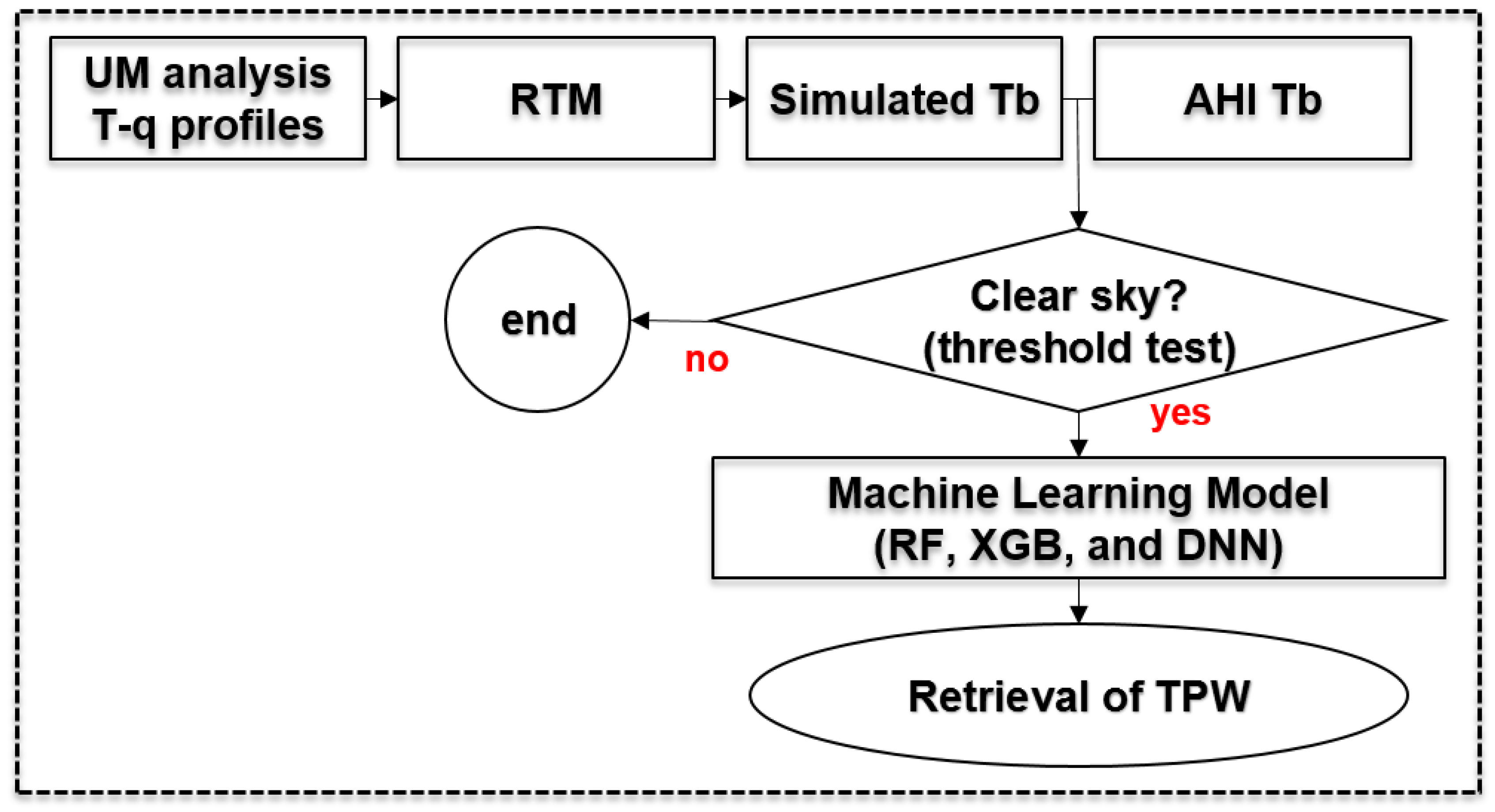
3. Methods
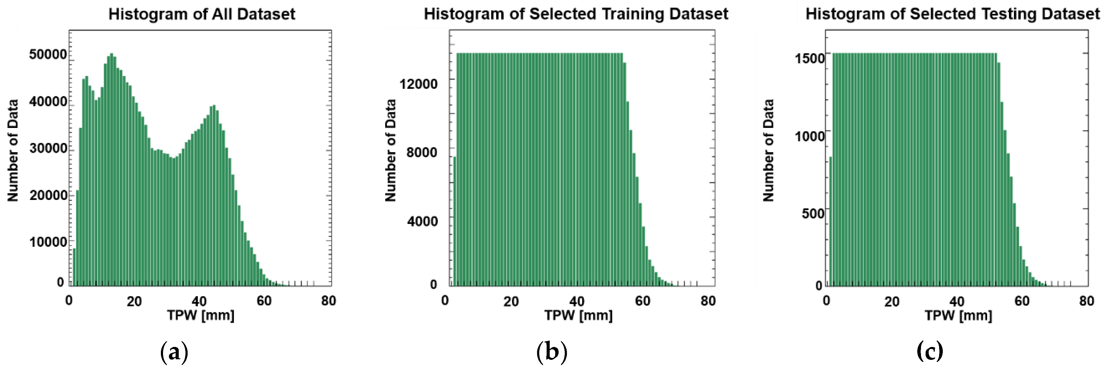
3.1. Preparation of Training Dataset
3.2. Machine Learning Approaches
3.3. Accuracy Metrics
4. Results and Discussion
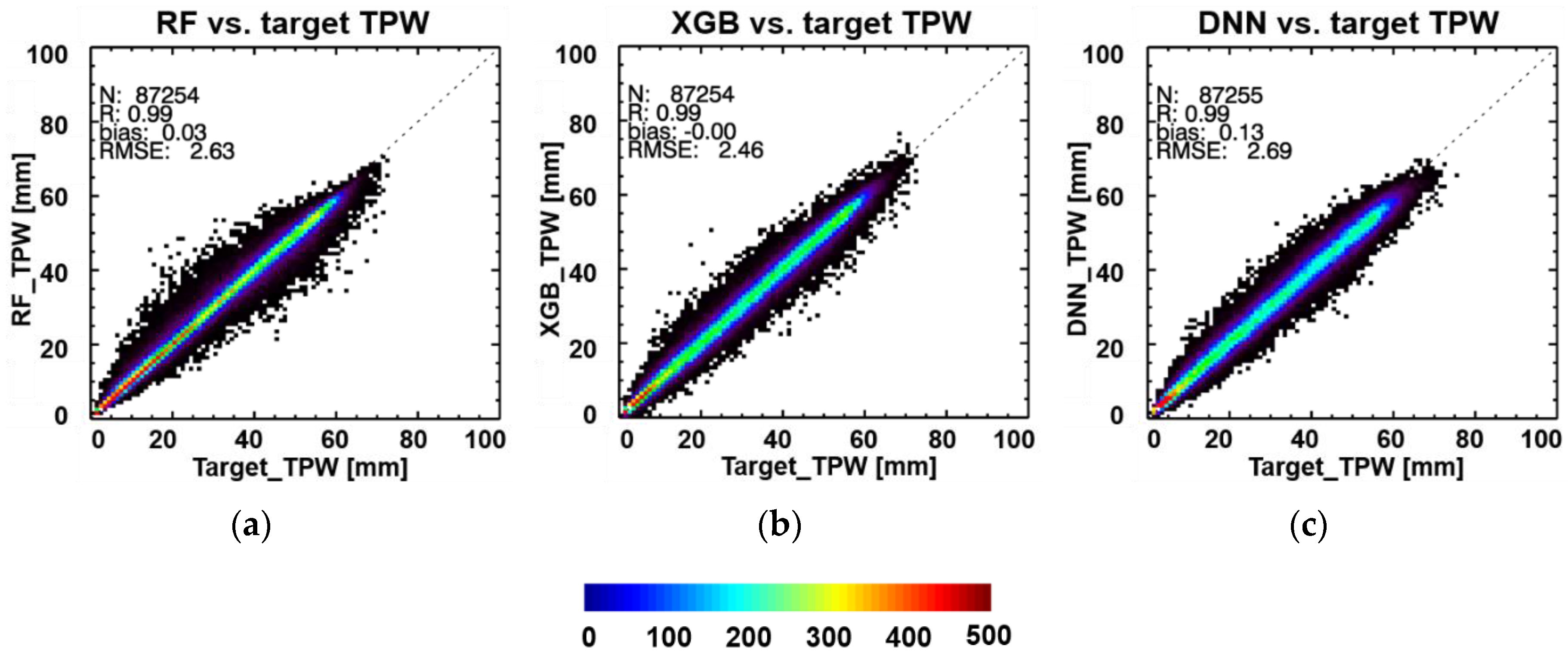
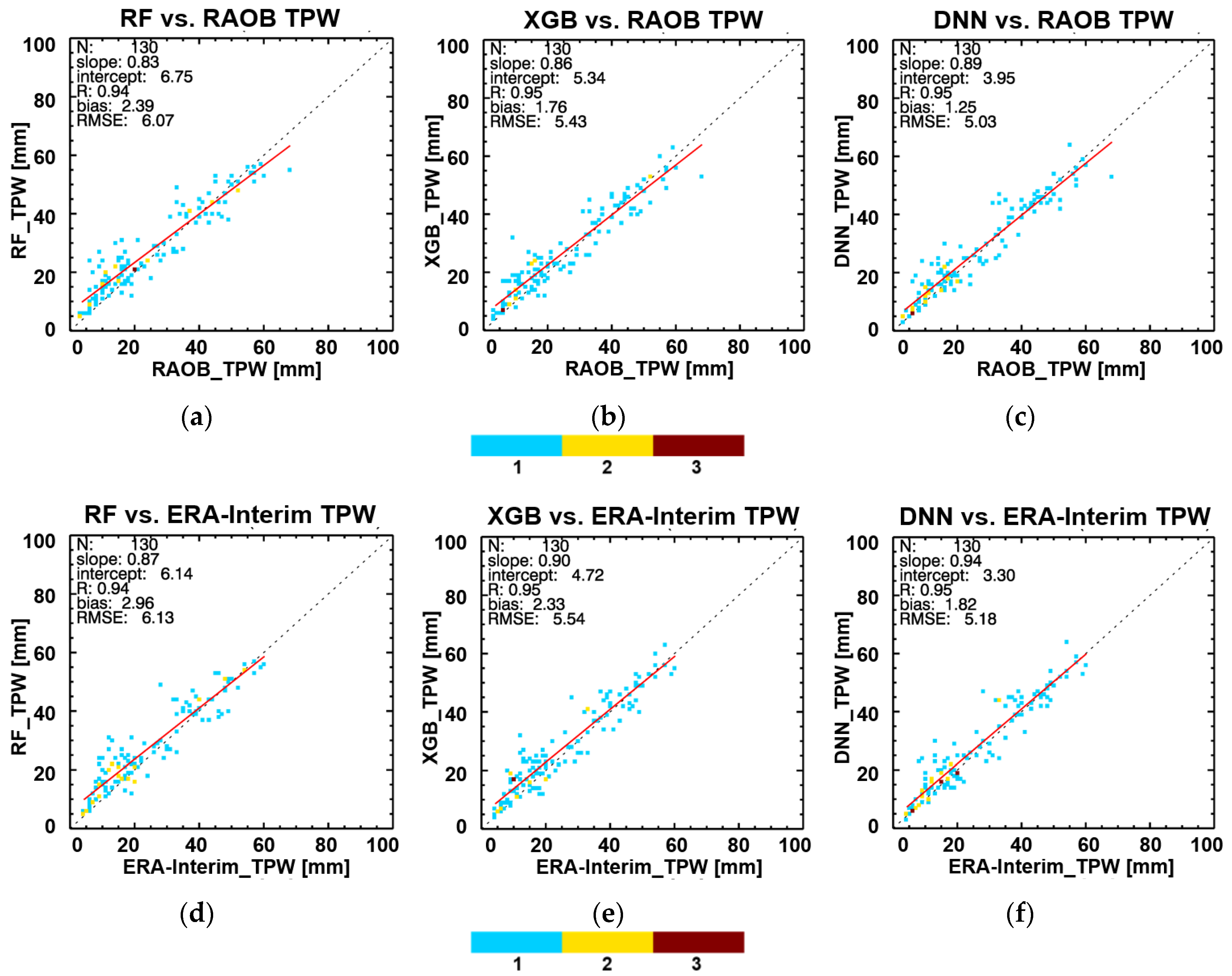
4.1. Model Performance
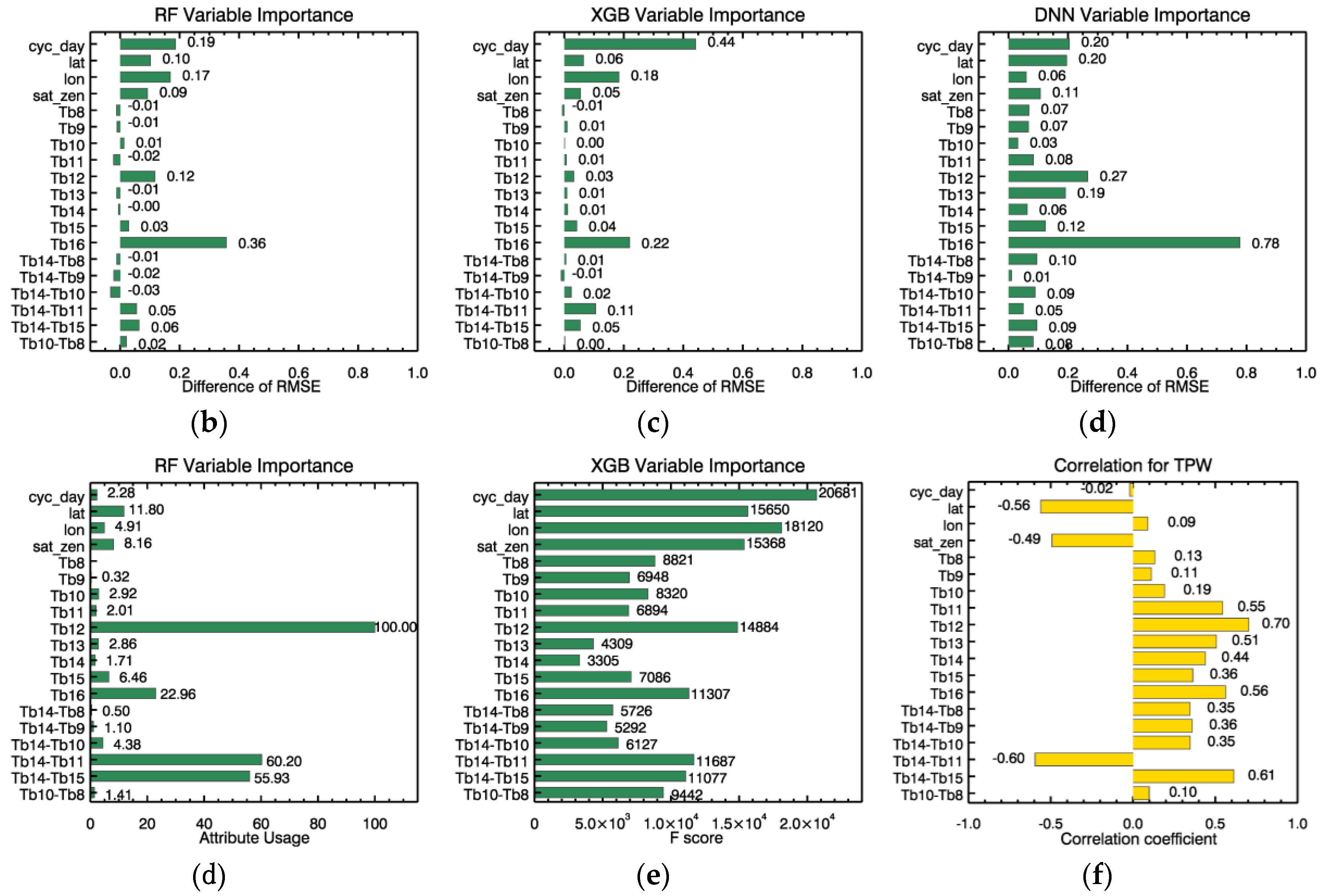
4.2. Variable Importance
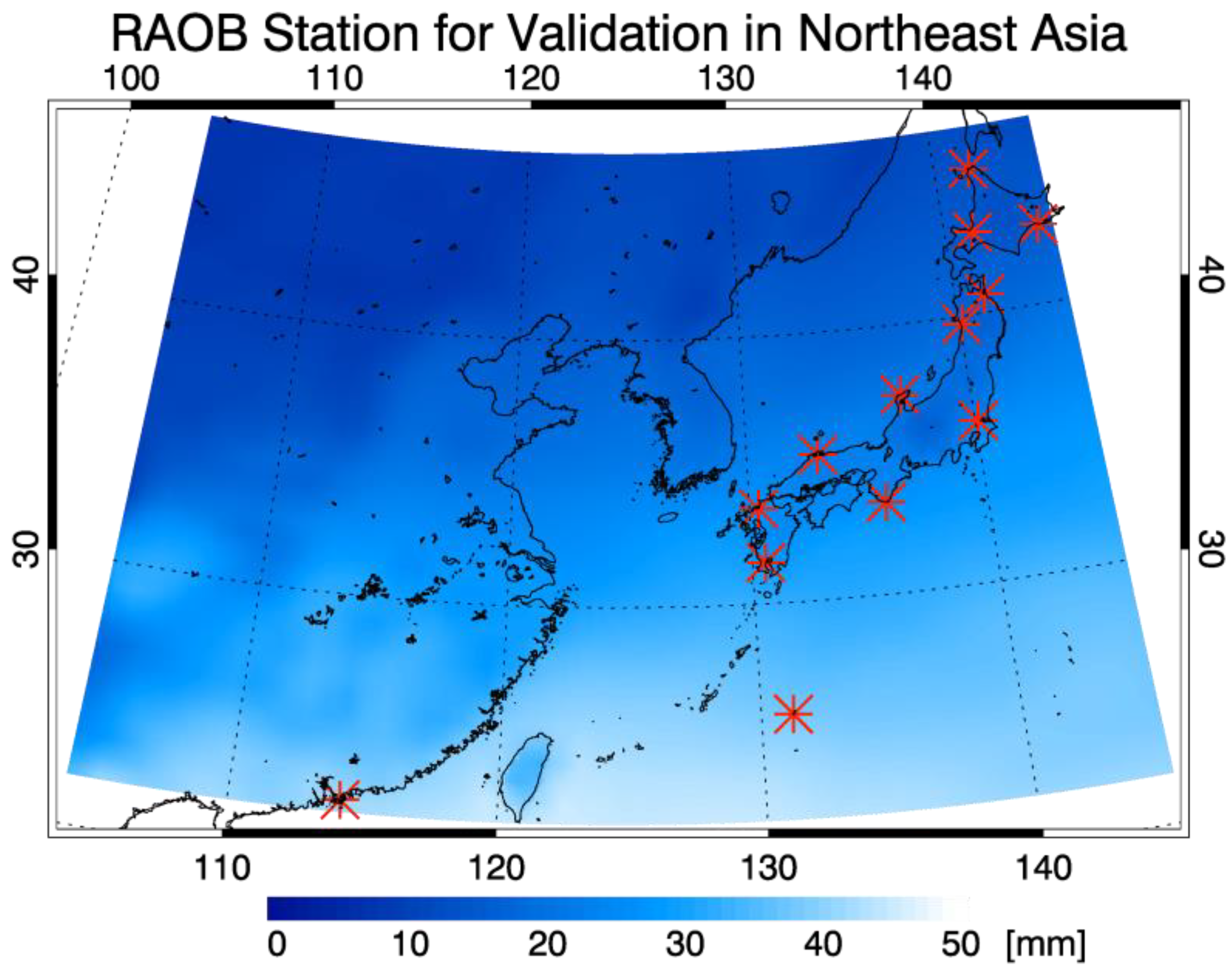
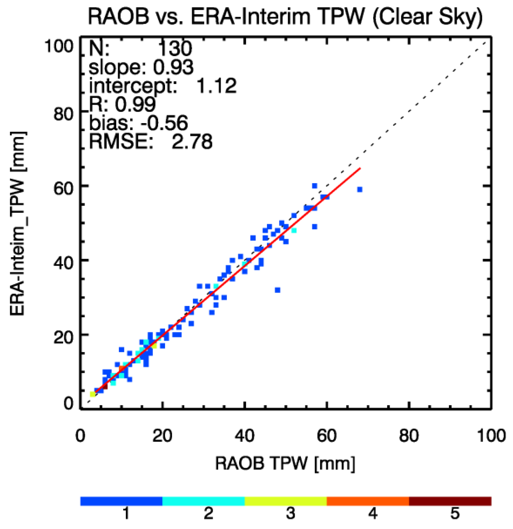
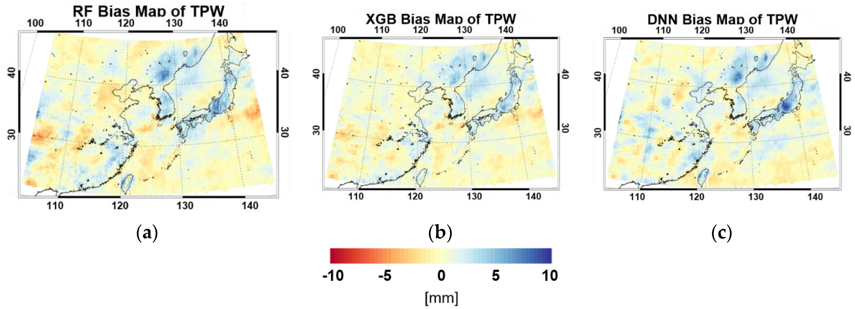
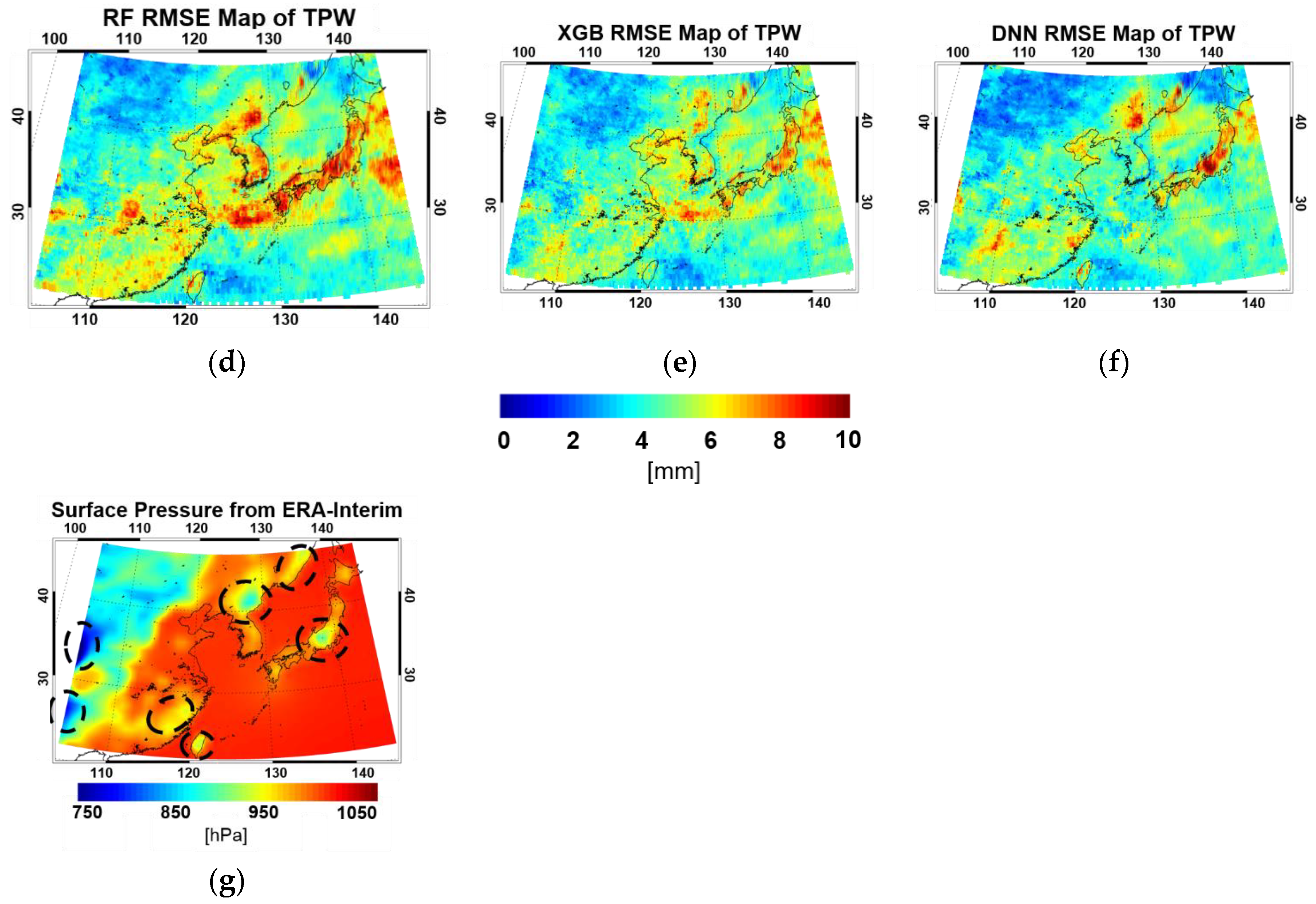
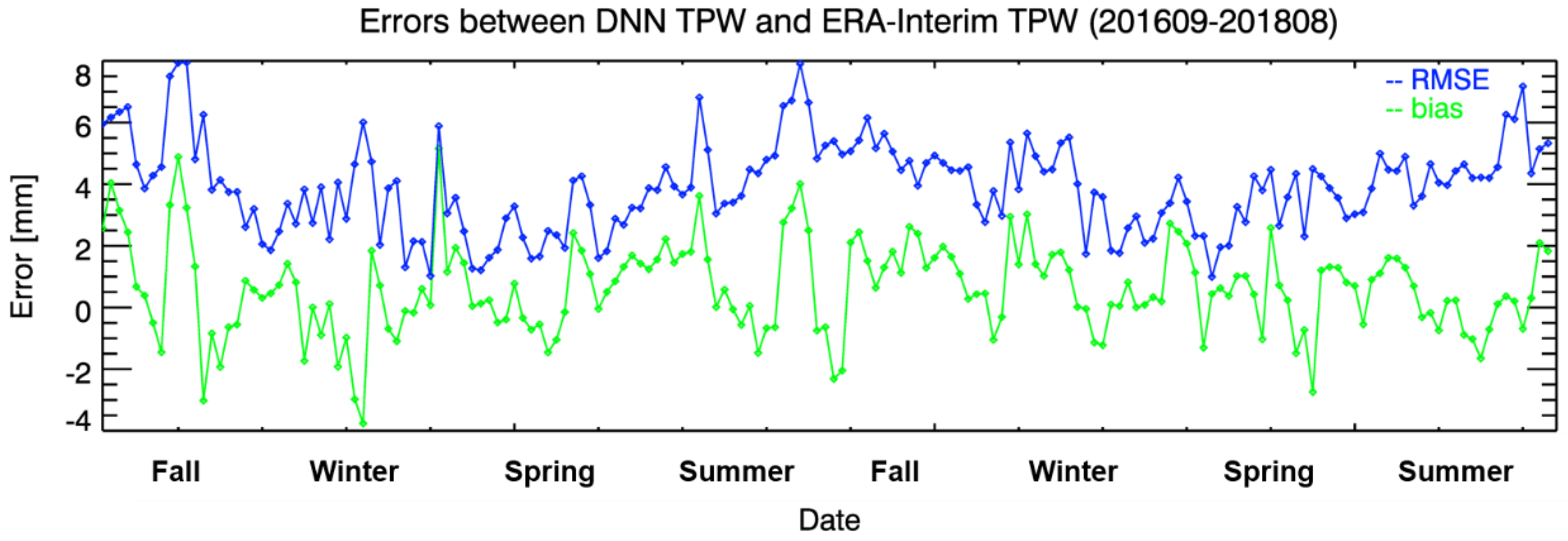
4.3. Validation Results
4.4. Novelty and Limitations
5. Conclusions
Author Contributions
Funding
Conflicts of Interest
References
- Trenberth, K.E.; Dai, A.; Rasmussen, R.M.; Parsons, D.B. The changing character of precipitation. Bull. Am. Meteorol. Soc. 2003, 84, 1205–1218. [Google Scholar] [CrossRef]
- Viswanadham, Y. The relationship between total precipitable water and surface dew point. J. Appl. Meteorol. 1981, 20, 3–8. [Google Scholar] [CrossRef]
- Manning, T.; Zhang, K.; Rohm, W.; Choy, S.; Hurter, F. Detecting severe weather using GPS tomography: An Australian case study. J. Glob. Position. Syst. 2012, 11, 58–70. [Google Scholar] [CrossRef]
- Lee, S.J.; Ahn, M.H.; Lee, Y. Application of an artificial neural network for a direct estimation of atmospheric instability from a next-generation imager. Adv. Atmos. Sci. 2016, 33, 221–232. [Google Scholar] [CrossRef]
- Bessho, K.; Date, K.; Hayashi, M.; Ikeda, A.; Imai, T.; Inoue, H.; Inoue, H.; Kumagai, Y.; Miyakwa, T.; Murata, H.; et al. An introduction to Himawari-8/9—Japan’s new-generation geostationary meteorological satellites. J. Meteorol. Soc. Jpn. 2016, 94, 151–183. [Google Scholar] [CrossRef]
- Martinez, M.A.; Velazquez, M.; Manso, M.; Mas, I. Application of LPW and SAI SAFNWC/MSG satellite products in pre-convective environments. Atmos. Res. 2007, 83, 366–379. [Google Scholar] [CrossRef]
- Liu, Z.; Min, M.; Li, J.; Sun, F.; Di, D.; Ai, Y.; Li, Z.; Qin, D.; Li, G.; Lin, Y.; et al. Local Severe Storm Tracking and Warning in Pre-Convection Stage from the New Generation Geostationary Weather Satellite Measurements. Remote Sens. 2019, 11, 383. [Google Scholar] [CrossRef]
- Lee, Y.K.; Li, J.; Li, Z.; Schmit, T. Atmospheric temporal variations in the pre-landfall environment of typhoon Nangka (2015) observed by the Himawari-8 AHI. Asia-Pac. J. Atmos. Sci. 2017, 53, 431–443. [Google Scholar] [CrossRef]
- Lee, S.J.; Ahn, M.-H.; Chung, S.-R. Atmospheric Profile Retrieval Algorithm for Next Generation Geostationary Satellite of Korea and Its Application to the Advanced Himawari Imager. Remote Sens. 2017, 9, 1294. [Google Scholar] [CrossRef]
- Wan, Z.; Dozier, J.A. Generalized split-window algorithm for retrieving land-surface temperature from space. IEEE Trans. Geosci. Remote Sens. 1996, 34, 892–905. [Google Scholar] [CrossRef]
- Tang, B.; Bi, Y.; Li, Z.L.; Xia, J. Generalized split-window algorithm for estimate of land surface temperature from Chinese geostationary FengYun meteorological satellite (FY-2C) data. Sensors 2008, 8, 933–951. [Google Scholar] [CrossRef] [PubMed]
- Chesters, D.; Robinson, W.D.; Uccellini, L.W. Optimized retrievals of precipitable water from the VAS “Split Window”. J. Appl. Meteorol. Climatol. 1987, 26, 1059–1066. [Google Scholar] [CrossRef]
- Dalu, G. Satellite remote sensing of atmospheric water vapour. Int. J. Remote Sens. 1986, 7, 1089–1097. [Google Scholar] [CrossRef]
- Sobrino, J.A.; Jimenez, J.C.; Raissouni, N.; Soria, G. A simplified method for estimating the total water vapor content over sea surfaces using NOAA-AVHRR channels 4 and 5. IEEE Trans. Geosci. Remote Sens. 2002, 40, 357–361. [Google Scholar] [CrossRef]
- Schroedter-Homscheidt, M.; Drews, A.; Heise, S. Total water vapor column retrieval from MSG-SEVIRI split window measurements exploiting the daily cycle of land surface temperatures. Remote Sens. Environ. 2008, 112, 249–258. [Google Scholar] [CrossRef]
- Barton, I.J.; Prata, A.J. Difficulties associated with the application of covariance–variance techniques to retrieval of atmospheric water vapor from satellite imagery. Remote Sens. Environ. 1999, 69, 76–83. [Google Scholar] [CrossRef]
- Knabb, R.D.; Fuelberg, H.E. A comparison of the first-guess dependence of precipitable water estimates from three techniques using GOES data. J. Appl. Meteorol. 1997, 36, 417–427. [Google Scholar] [CrossRef]
- Nielsen, M.A. Neural Networks and Deep Learning; Determination Press: San Francisco, CA, USA, 2015; Available online: http://neuralnetworksanddeeplearning.com/ (accessed on 29 December 2017).
- Wang, W.; Sun, X.; Zhang, R.; Li, Z.; Zhu, Z.; Su, H. Multi-layer perceptron neural network based algorithm for estimating precipitable water vapour from MODIS NIR data. Int. J. Remote Sens. 2006, 27, 617–621. [Google Scholar] [CrossRef]
- Zhang, S.L.; Xu, L.S.; Ding, J.L.; Liu, H.L.; Deng, X.B. Precipitable Water Vapor Retrieval Using Neural Network from Infrared Hyperspectral Soundings. Key Eng. Mater. 2012, 500, 390–396. [Google Scholar] [CrossRef]
- Lee, Y.-K.; Li, Z.; Li, J. Evaluation of the GOES-R ABI LAP Retrieval Algorithm Using the GOES-13 Sounder. J. Atmos. Ocean. Technol. 2014, 31, 3–19. [Google Scholar] [CrossRef]
- Dee, D.P.; Uppala, S.M.; Simmons, A.J.; Berrisford, P.; Poli, P.; Kobayashi, S.; Andrae, U.; Balmaseda, M.A.; Balsamo, G.; Bauer, P.; et al. The ERA-Interim reanalysis: Configuration and performance of the data assimilation system. Q. J. R. Meteorol. Soc. 2011, 137, 553–597. [Google Scholar] [CrossRef]
- Basili, P.; Bonafoni, S.; Mattioli, V.; Pelliccia, F.; Ciotti, P.; Carlesimo, G.; Pierdicca, N.; Venuti, G.; Mazzoni, A. Neural-network retrieval of integrated precipitable water vapor over land from satellite microwave radiometer. In Proceedings of the 2010 11th Specialist Meeting on Microwave Radiometry and Remote Sensing of the Environment IEEE, Washington, DC, USA, 1–4 March 2010; pp. 161–166. [Google Scholar] [CrossRef]
- Bonafoni, S.; Mattioli, V.; Basili, P.; Ciotti, P.; Pierdicca, N. Satellite-based retrieval of precipitable water vapor over land by using a neural network approach. IEEE Trans. Geosci. Remote Sens. 2011, 49, 3236–3248. [Google Scholar] [CrossRef]
- Ingleby, B. On the Accuracy of Different Radiosonde Types–ECMWF. TECO-2016 Madrid, 30 September 2016. Available online: https://www.wmo.int/pages/prog/www/IMOP/publications/IOM-125_TECO_2016/Session_4/O4(8)_pres_Ingleby_TECO_types_4_8.pdf (accessed on 7 May 2019).
- Ebell, K.; Orlandi, E.; Hünerbein, A.; Löhnert, U.; Crewell, S. Combining ground-based with satellite-based measurements in the atmospheric state retrieval: Assessment of the information content. J. Geophys. Res. Atmos. 2013, 118, 6940–6956. [Google Scholar] [CrossRef]
- Lee, S.J.; Ahn, M.H.; Ha, S. Total Column Ozone Retrieval From the Infrared Measurements of a Geostationary Imager. IEEE Trans. Geosci. Remote Sens. 2019, 1–9. [Google Scholar] [CrossRef]
- Zhou, L.; Pan, S.; Wang, J.; Vasilakos, A.V. Machine learning on big data: Opportunities and challenges. Neurocomputing 2017, 237, 350–361. [Google Scholar] [CrossRef]
- Karahoca, A. Advances in Data Mining Knowledge Discovery and Applications; InTech: Rijeka, Croatia, 2012; ISBN 978-953-51-0748-4. [Google Scholar] [CrossRef]
- Yu, L.; Wang, S.; Lai, K.K. An integrated data preparation scheme for neural network data analysis. IEEE Trans. Knowl. Data Eng. 2006, 18, 217–230. [Google Scholar] [CrossRef]
- Amani, M.; Salehi, B.; Mahdavi, S.; Granger, J.; Brisco, B. Wetland classification in Newfoundland and Labrador using multi-source SAR and optical data integration. GISci. Remote Sens. 2017, 54, 779–796. [Google Scholar] [CrossRef]
- Liu, T.; Abd-Elrahman, A.; Morton, J.; Wilhelm, V.L. Comparing fully convolutional networks, random forest, support vector machine, and patch-based deep convolutional neural networks for object-based wetland mapping using images from small unmanned aircraft system. GISci. Remote Sens. 2018, 55, 243–264. [Google Scholar] [CrossRef]
- Guo, Z.; Du, S. Mining parameter information for building extraction and change detection with very high-resolution imagery and GIS data. GISci. Remote Sens. 2017, 54, 38–63. [Google Scholar] [CrossRef]
- Richardson, H.J.; Hill, D.J.; Denesiuk, D.R.; Fraser, L.H. A comparison of geographic datasets and field measurements to model soil carbon using random forests and stepwise regressions (British Columbia, Canada). GISci. Remote Sens. 2017, 54, 573–591. [Google Scholar] [CrossRef]
- Forkuor, G.; Dimobe, K.; Serme, I.; Tondoh, J.E. Landsat-8 vs. Sentinel-2: Examining the added value of sentinel-2’s red-edge bands to land-use and land-cover mapping in Burkina Faso. GISci. Remote Sens. 2018, 55, 331–354. [Google Scholar] [CrossRef]
- Georganos, S.; Grippa, T.; Vanhuysse, S.; Lennert, M.; Shimoni, M.; Kalogirou, S.; Wolff, E. Less is more: Optimizing classification performance through feature selection in a very-high-resolution remote sensing object-based urban application. GISci. Remote Sens. 2018, 55, 221–242. [Google Scholar] [CrossRef]
- Zhang, C.; Smith, M.; Fang, C. Evaluation of Goddard’s LiDAR, hyperspectral, and thermal data products for mapping urban land-cover types. GISci. Remote Sens. 2018, 55, 90–109. [Google Scholar] [CrossRef]
- Sonobe, R.; Yamaya, Y.; Tani, H.; Wang, X.; Kobayashi, N.; Mochizuki, K.I. Assessing the suitability of data from Sentinel-1A and 2A for crop classification. GISci. Remote Sens. 2017, 54, 918–938. [Google Scholar] [CrossRef]
- Santos, L.D. GPU Accelerated Classifier Benchmarking for Wildfire Related Tasks. Ph.D. Thesis, NOVA University of Lisbon, Lisbon, Portugal, 2018. Available online: https://run.unl.pt/handle/10362/61547 (accessed on 11 May 2019).
- Nisa, I.; Siegel, C.; Rajam, A.S.; Vishnu, A.; Sadayappan, P. Effective Machine Learning Based Format Selection and Performance Modeling for SpMV on GPUs. In Proceedings of the 2018 IEEE International Parallel and Distributed Processing Symposium Workshops (IPDPSW), Vancouver, BC, Canada, 21–25 May 2018; pp. 1056–1065. [Google Scholar]
- Babajide Mustapha, I.; Saeed, F. Bioactive molecule prediction using extreme gradient boosting. Molecules 2016, 21, 983. [Google Scholar] [CrossRef] [PubMed]
- Yang, J.; Guo, A.; Li, Y.; Zhang, Y.; Li, X. Simulation of landscape spatial layout evolution in rural-urban fringe areas: A case study of Ganjingzi District. GISci. Remote Sens. 2019, 56, 388–405. [Google Scholar] [CrossRef]
- Omrani, H.; Tayyebi, A.; Pijanowski, B. Integrating the multi-label land-use concept and cellular automata with the artificial neural network-based Land Transformation Model: An integrated ML-CA-LTM modeling framework. GISci. Remote Sens. 2017, 54, 283–304. [Google Scholar] [CrossRef]
- Antonanzas, J.; Urraca, R.; Aldama, A.; Fernández-Jiménez, L.A.; Martínez-de-Pisón, F.J. Single and Blended Models for Day-Ahead Photovoltaic Power Forecasting; Springer International Publishing: La Rioja, Spain, 2017; pp. 427–434. ISBN 978-3-319-59649-5. [Google Scholar]
- Pan, B. Application of XGBoost algorithm in hourly PM2.5 concentration prediction. In Proceedings of the IOP Conference Series: Earth and Environmental Science, Harbin, China, 8–10 February 2018. [Google Scholar]
- Just, A.; De Carli, M.; Shtein, A.; Dorman, M.; Lyapustin, A.; Kloog, I. Correcting Measurement Error in Satellite Aerosol Optical Depth with Machine Learning for Modeling PM2.5 in the Northeastern USA. Remote Sens. 2018, 10, 803. [Google Scholar] [CrossRef]
- EUMETSAT. Product Tutorial on Total Precipitable Water Content Products. 2014. Available online: http://www.eumetrain.org/data/3/359/print_3.htm#page_1.0.0 (accessed on 5 May 2019).
- Hocking, J.; Rayer, P.; Saunders, R.; Madricardi, M.; Geer, A.; Brunel, P.; Vidot, J. RTTOV v11 Users Guide. NWP SAF, Version 1.4. September 2015. Available online: https://www.nwpsaf.eu/site/download/documentation/rtm/docs_rttov11/users_guide_11_v1.4.pdf (accessed on 5 July 2019).
- Breiman, L. Random forests. Mach. Learn. 2001, 45, 5–32. [Google Scholar] [CrossRef]
- Wright, M.N.; Ziegler, A. Ranger: A fast implementation of random forests for high dimensional data in C++ and R. J. Stat. Softw. 2017, 77. [Google Scholar] [CrossRef]
- Chen, T.; Guestrin, C. XGBoost: A Scalable Tree Boosting System. In Proceedings of the 22nd ACM Sigkdd International Conference on Knowledge Discovery and Data Mining, San Francisco, CA, USA, 13–17 August 2016; pp. 785–794. [Google Scholar]
- Dewancker, I.; McCourt, M.; Clark, S. Bayesian Optimization Primer. 2015. Available online: https://app.sigopt.com/static/pdf/SigOpt_Bayesian_Optimization_Primer.pdf (accessed on 11 May 2019).
- Blackwell, W.J.; Chen, F.W. Neural Networks in Atmospheric Remote Sensing; Artech House: Norwood, MA, USA, 2009; p. 234. ISBN 978-1-59693-372-9. [Google Scholar]
- Bengio, Y.; Grandvalet, Y. No unbiased estimator of the variance of k-fold cross-validation. J. Mach. Learn. Res. 2004, 5, 1089–1105. [Google Scholar]
- Khalid, S.; Khalil, T.; Nasreen, S. A survey of feature selection and feature extraction techniques in machine learning. In Proceedings of the Science and Information Conference (SAI), London, UK, 27–29 August 2014. [Google Scholar]
- Mears, C.A.; Santer, B.D.; Wentz, F.J.; Taylor, K.E.; Wehner, M.F. Relationship between temperature and precipitable water changes over tropical oceans. Geophys. Res. Lett. 2007, 34. [Google Scholar] [CrossRef]
- Noh, Y.-C.; Sohn, B.-J.; Kim, Y.; Joo, S.; Bell, W. Evaluation of Temperature and Humidity Profiles of Unified Model and ECMWF Analyses Using GRUAN Radiosonde Observations. Atmosphere 2016, 7, 94. [Google Scholar] [CrossRef]
- Bastani, O.; Ioannou, Y.; Lampropoulos, L.; Vytiniotis, D.; Nori, A.; Criminisi, A. Measuring Neural Net Robustness with Constraints; Curran Associates Inc.: Red Hook, NY, USA, 2016; pp. 2613–2621. ISBN 978-1-5108-3881-9. [Google Scholar]
- Shalev-Shwartz, S. Online learning and online convex optimization. Found. Trends® Mach. Learn. 2012, 4, 107–194. [Google Scholar] [CrossRef]


| Channel Number | Central Wavelength | Band Width | Spatial Resolution at Sub Satellite Point (km) |
|---|---|---|---|
| 1 | 0.47 | 0.05 | 1 |
| 2 | 0.51 | 0.02 | 1 |
| 3 | 0.64 | 0.03 | 0.5 |
| 4 | 0.86 | 0.02 | 1 |
| 5 | 1.6 | 0.02 | 2 |
| 6 | 2.3 | 0.02 | 2 |
| 7 | 3.9 | 0.22 | 2 |
| 8 | 6.2 | 0.37 | 2 |
| 9 | 6.9 | 0.12 | 2 |
| 10 | 7.3 | 0.17 | 2 |
| 11 | 8.6 | 0.32 | 2 |
| 12 | 9.6 | 0.18 | 2 |
| 13 | 10.4 | 0.30 | 2 |
| 14 | 11.2 | 0.20 | 2 |
| 15 | 12.4 | 0.30 | 2 |
| 16 | 13.3 | 0.20 | 2 |
| Reference Data | Temporal and Spatial Resolution | Period and Usage |
|---|---|---|
| ERA-Interim | 6 h/ 0.125° × 0.125° | September 2016–August 2018 Four days per month (5th, 10th, 15th, 20th) Training data (90%)/test data (10%) |
| September 2016–August 2018 Two days per month (1st, 25th) Validation data | ||
| RAOB | 12 h 1/ 13 sites over Northeast Asia | September 2016–August 2018 Two days per month (1st, 25th) Validation data |
| Input Variable | Physical Characteristics |
|---|---|
| Cyclic_day | Temporal characteristics |
| Latitude | Spatial characteristics |
| Longitude | Spatial characteristics |
| Satellite zenith angle | Optical depth |
| BT8 (IR 6.2 ) | Upper tropospheric water vapor |
| BT9 (IR 6.9 ) | Mid and upper tropospheric water vapor |
| BT10 (IR 7.3 ) | Mid tropospheric water vapor |
| BT11 (IR 8.6 ) | Total water for stability, dust, SO2, rainfall |
| BT12 (IR 9.63 ) | Total ozone |
| BT13 (IR 10.4 ) | Surface |
| BT14 (IR 11.2 ) | Sea surface temperature and rainfall |
| BT15 (IR 12.4 ) | Total water and SST |
| BT16 (IR 13.3 ) | Air temperature |
| DCD BT14−BT8 | Upper tropospheric moisture |
| DCD BT14−BT9 | Mid and upper tropospheric moisture |
| DCD BT14−BT10 | Mid tropospheric moisture |
| DCD BT14−BT11 | Amount of water vapor |
| DCD BT14−BT15 | Split-window channels (amount of water vapor) |
| DCD BT10−BT8 | Difference between water vapor channels |
| Reference Data | Temporal Resolution | Spatial Resolution | Collocation Criteria |
|---|---|---|---|
| ERA-Interim | 6 h | 0.125° × 0.125° | Averaging one or more retrieved TPW within a 0.1-degree radius |
| RAOB | 12 h 1 | 13 sites over Northeast Asia | Averaging one or more retrieved TPW within a 0.1-degree radius |
| All | Land | Sea | Coast | |||||
|---|---|---|---|---|---|---|---|---|
| bias | RMSE | bias | RMSE | bias | RMSE | bias | RMSE | |
| RF | 0.62 | 5.09 | 0.66 | 4.94 | 0.55 | 5.29 | 0.88 | 5.98 |
| XGB | 0.70 | 4.85 | 0.67 | 4.63 | 0.72 | 5.14 | 1.04 | 5.65 |
| DNN | 0.90 | 4.65 | 0.94 | 4.50 | 0.83 | 4.86 | 1.20 | 5.22 |
© 2019 by the authors. Licensee MDPI, Basel, Switzerland. This article is an open access article distributed under the terms and conditions of the Creative Commons Attribution (CC BY) license (http://creativecommons.org/licenses/by/4.0/).
Share and Cite
Lee, Y.; Han, D.; Ahn, M.-H.; Im, J.; Lee, S.J. Retrieval of Total Precipitable Water from Himawari-8 AHI Data: A Comparison of Random Forest, Extreme Gradient Boosting, and Deep Neural Network. Remote Sens. 2019, 11, 1741. https://doi.org/10.3390/rs11151741
Lee Y, Han D, Ahn M-H, Im J, Lee SJ. Retrieval of Total Precipitable Water from Himawari-8 AHI Data: A Comparison of Random Forest, Extreme Gradient Boosting, and Deep Neural Network. Remote Sensing. 2019; 11(15):1741. https://doi.org/10.3390/rs11151741
Chicago/Turabian StyleLee, Yeonjin, Daehyeon Han, Myoung-Hwan Ahn, Jungho Im, and Su Jeong Lee. 2019. "Retrieval of Total Precipitable Water from Himawari-8 AHI Data: A Comparison of Random Forest, Extreme Gradient Boosting, and Deep Neural Network" Remote Sensing 11, no. 15: 1741. https://doi.org/10.3390/rs11151741
APA StyleLee, Y., Han, D., Ahn, M.-H., Im, J., & Lee, S. J. (2019). Retrieval of Total Precipitable Water from Himawari-8 AHI Data: A Comparison of Random Forest, Extreme Gradient Boosting, and Deep Neural Network. Remote Sensing, 11(15), 1741. https://doi.org/10.3390/rs11151741