LEO to GEO-SAR Interferences: Modelling and Performance Evaluation

Abstract

This paper proposes a statistical model to evaluate the impact of the signal backscattered by low Earth orbiting (LEO) synthetic aperture radar (SAR) and received by GEO-stationary orbiting SAR. The model properly accounts for the bistatic backscatter, the number of LEO-SAR satellites and their duty cycles. The presence of many sun-synchronous, dawn-dusk satellites creates a 24 h periodic pattern in interference that should be considered in the acquisition plan of future geostationary SAR. The model, implemented by a numerical simulator, allows also the prediction of performance in future scenarios of many LEO-SAR. Examples and evaluations are made here for X band.

1. Introduction

Geosynchronous synthetic aperture radar (SAR) are acquiring momentum due to their capability to perform imaging over wide areas with a revisit otherwise impossible with low Earth orbiting (LEO) or medium Earth orbiting (MEO) SAR [1,2,3,4]. In particular, the concept of a geostationary orbiting SAR, that should fulfill ITU requirements allowing a slight, non-zero eccentricity orbit to provide a synthetic aperture, is quite attractive for their capability of near-continuous imaging. Images are obtained by integrating over long intervals, up to hours, to compensate for the huge spread losses, while enabling the use of current technologies in terms of power and antenna reflectors [4,5,6].

Nearly half of the Earth’s surface is seen from Geostationary (GEO) orbit under a small angular aperture of ~19°: this is the key to fast, super-continental access, but at the same time, it exposes these systems to many potential radio frequency interferences (RFI) coming from anywhere. In [7], the impact of disturbances coming from on-ground, or due to the signal back-scattered from LEO-SAR, has been analyzed under very general assumptions. It has been shown that C and X band systems are more promising than L band due to the lower population of RFI and higher antenna directivity.

The balance between ground and LEO RFI is different in the two frequencies: the C-band systems are more subject to on-ground RFI, since the band is open to ground services like weather radar [8,9], whereby X band is primarily allocated to ESS-Active (Exploration Satellite Service), that should, in principle, exclude on-ground RFI. However, the number of present and future X band SARs, like the forthcoming constellations of light SARs: ICEYE, Capella Space or UmbraLab, is so large to motivate the in-depth analysis performed in the paper, and the need for a performance model capable of adapting to present and future scenarios. While the numeric evaluations are here performed in X band, the methodology developed can be extended to any frequency.

The paper is organized as follows: Section 2 provides the model for estimating the mean power scattered by the terrain, illuminated by the LEO-SAR, and captured by the GEO-SAR. Section 3 provides a statistical characterization of that backscatter, made by analyzing the current LEO-SAR scenario. In Section 4 a performance evaluation is made as function of the hours of the day and the integration interval, i.e., accounting for the impact of many dawn-dusk satellites. Section 5 discusses possible mitigation approaches. The last two sections are about overall discussions and conclusions.

2. LEO-to-GEO RFI Evaluation

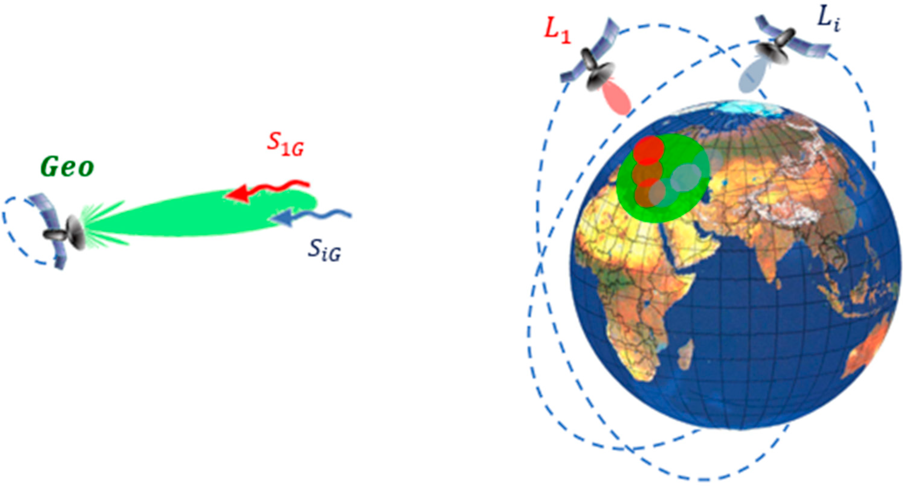
The geostationary radar geometry is sketched in Figure 1. The GEO-SAR, orbiting at about 42,000 km from Earth center, receives the contribution of its own backscatter, superposed to the backscatter originated by other N LEO satellites, L₁…L_N. As the GEO-SAR range is about 43 times that of LEO-SAR, its power density on the ground is expected to be ~43² = 1800 times lower than that of a LEO-SAR, by assuming the same transmitted power and antenna area. Therefore, it is unlikely that a GEO-SAR would disturb a LEO-SAR, but the opposite is a challenge for the GEO-SAR.

The evaluation of the signal to interference ratio (SIR) can carried out by comparing the backscattered echo power, as from Radar Equation [1,2,3,4,5,6,7], to the total RFI power. We assume that the GEO and LEO-SARs have uniform illumination and that transmit for all time the mean power, the product of peak power and the duty cycle. Notice that while the GEO-SAR is nearly stationary, the LEO-SAR moves by km/s, generating a fast time-varying disturbance.

The mean signal power received from GEO-SAR can be approximately expressed by assuming that all its mean power, $P_{Tg}$, is distributed to the ground beam surface (the wide green spot in Figure 1), then a fraction of this power, proportional to the mean monostatic backscatter coefficient ${\sigma }_G^0,$ is scattered back to the sensor, and partly gathered by the GEO-SAR antenna [4,5,6]:

$$P_G=P_{TG}·{\sigma }_G^0·\frac{1}{4\pi R_G^2}·\frac{{\lambda }^2}{4\pi }{G}_{G0}·{\eta }_T$$

(1)

where $R_G$ is the GEO-SAR range, ${\eta }_T$ the total losses, λ is the wavelength and $G_{G0}$ is the mean antenna directivity at the beam center (see Figure 2).

The mean RFI power received by the GEO-SAR and originated by the i-th LEO-SAR can be computed similarly to (1), but accounting for the fast time-variation of the LEO-SAR along its orbit:

$$P_i\left(t\right)=v_i\left(t\right)·r_i·d_i·P_{Ti}·\frac{{\sigma }^0\left({\theta }_{iL}\left(t\right),{\phi }_{iL}\left(t\right),{\theta }_{iG}\left(t\right),{\phi }_{iG}\left(t\right)\right)}{4\pi R_{iG}^2\left(t\right)}·\frac{{\lambda }^2}{4\pi }{G}_G\left({\theta }_{iG}\left(t\right),{\phi }_{iG}\left(t\right)\right)·{\eta }_T$$

(2)

The terms have the following meanings:

• v_i(t) is a binary (1/0), “visibility” index, set to one if the LEO-SAR is in the part of Earth accessible by GEO-SAR, that is, the field of view assumed in Figure 2;
• r_i is the ratio between GEO-SAR and LEO-SAR bandwidth;
• d_i is the LEO-SAR duty cycle along orbit;
• $P_{Ti}$ is the total LEO-SAR transmitted power;
• ${\sigma }^0\left({\theta }_{iL},{\phi }_{iL},{\theta }_{iG}\left(t\right),{\phi }_{iG}\left(t\right)\right)$ is the bistatic scatter coefficient from the i-th LEO-SAR direction, defined by incidence and azimuth angles ${\theta }_{iL},{\phi }_{iL}$ to the GEO-SAR one, defined by ${\theta }_{iG}\left(t\right),{\phi }_{iG}\left(t\right)$;
• $R_{iG}$ is the range from LEO-SAR scene center to GEO-SAR;
• $G_G\left({\theta }_{iG}\left(t\right),{\phi }_{iG}\left(t\right)\right)$ is the GEO-SAR antenna directivity to the LEO-SAR beam center, see Figure 2.

Note that we do assume the same losses in both GEO, in (1) and LEO, in (2), that is equivalent to ignore them as for the signal-to-interference ratio (SIR).

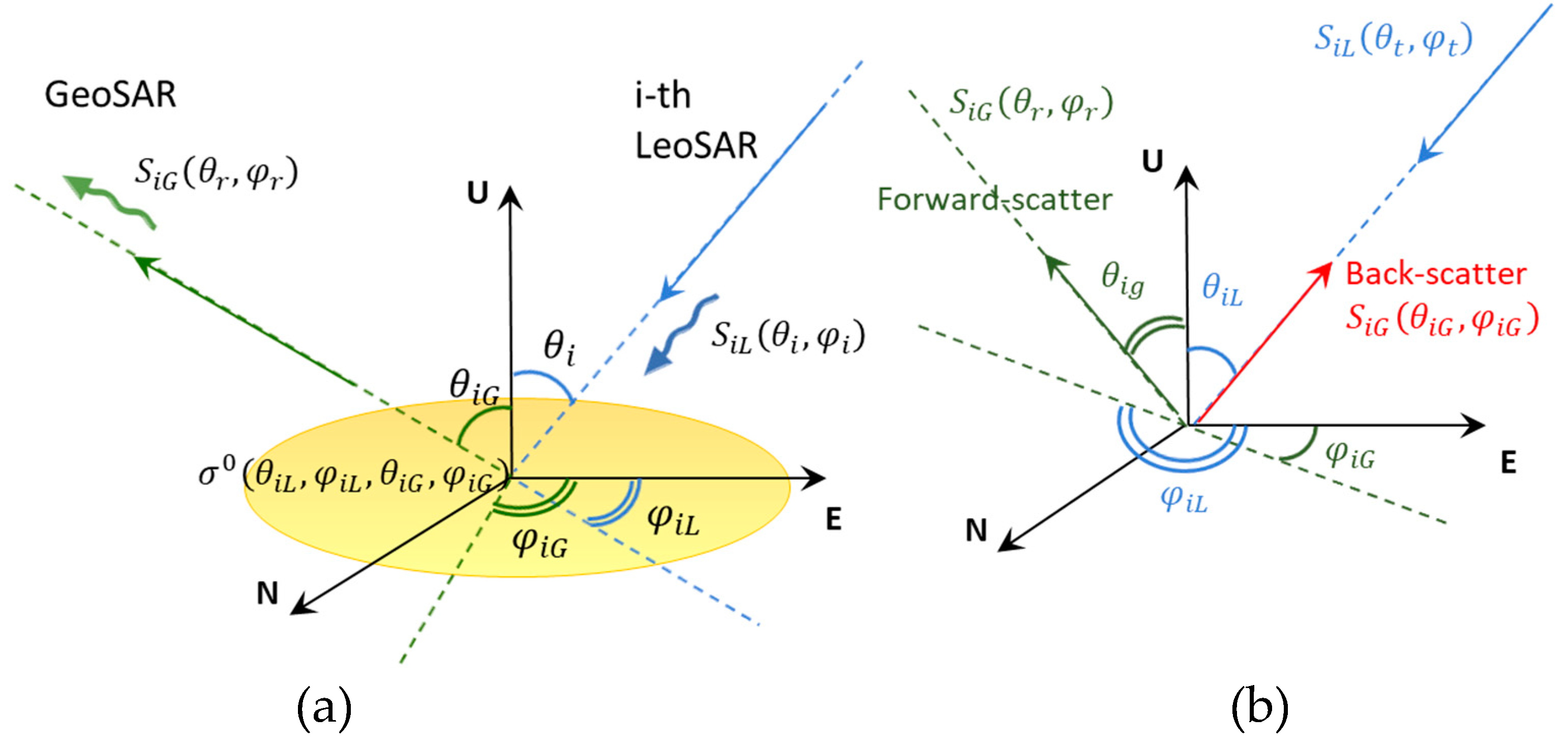
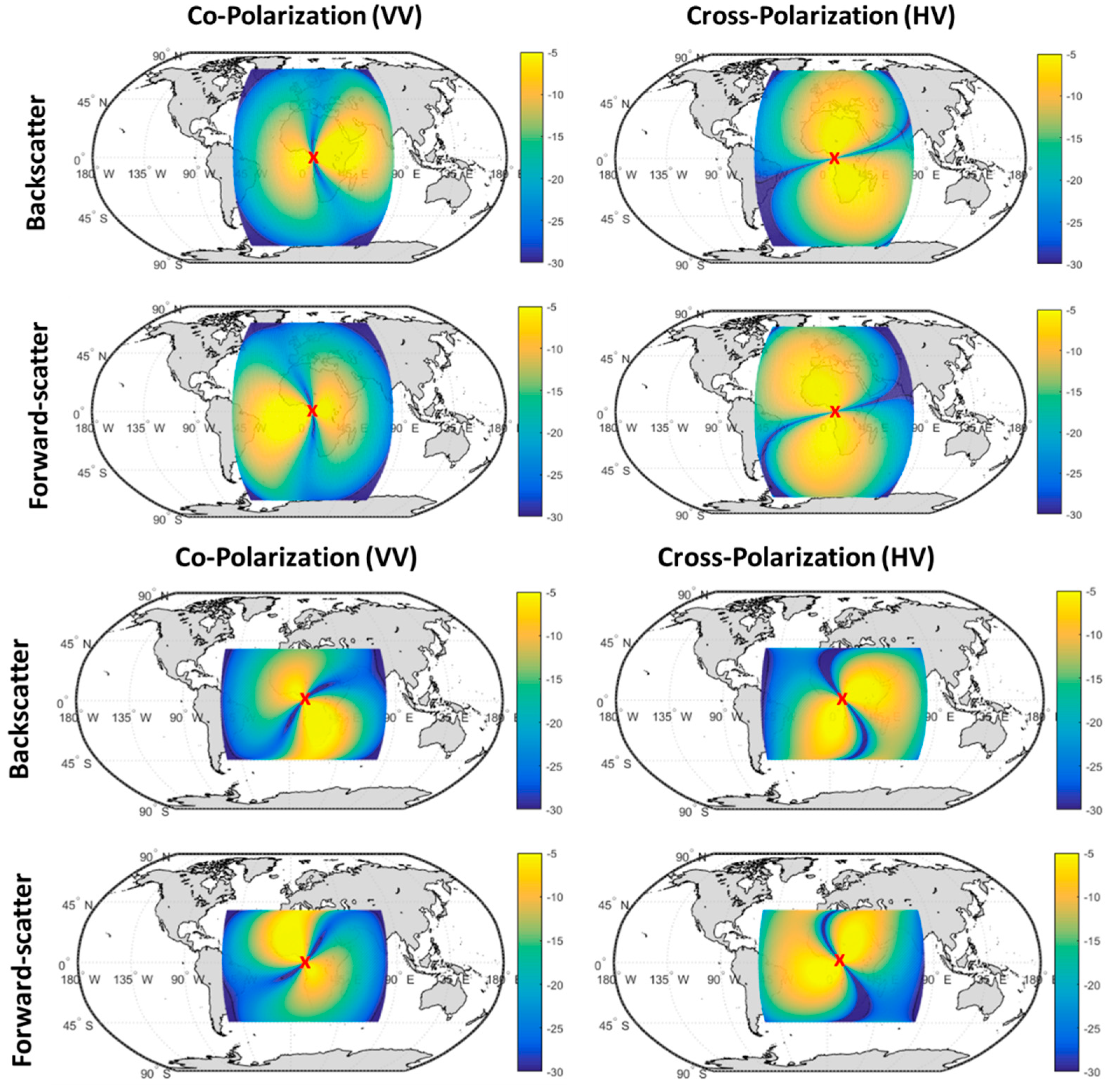
Bistatic Scattering

The LEO-to-GEO bistatic scattering, ${\sigma }^0$ in (2) is to be evaluated for the proper geometry, where the illumination from LEO-SAR, most of them being polar orbiting, is nearly orthogonal to the backscatter in the direction of the geostationary SAR, for which range is almost south-north. The change in backscatter plane, shown in Figure 3. on the left is a major difference respective to [7].

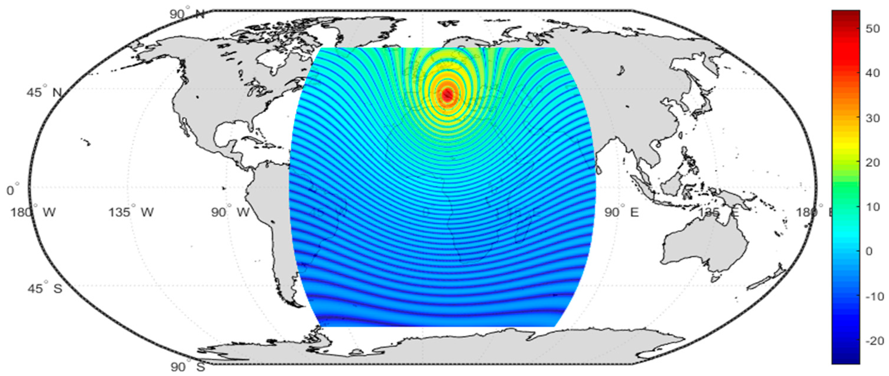
The actual ${\sigma }^0$ has been calculated by means of the Gilbert–Johnson model [10] for category ‘soil’, and assuming X band, see also [11], and mean incidence ${\theta }_{iL}=30°$. Examples of evaluation are shown in Figure 4 for different polarizations, scatter directions (back and forward, see Figure 3. on the right), and two LEO orbits: a 95° inclined, nearly polar one, and a 50° inclined nearly equatorial orbit.

We remark that the assumption of the ‘soil’ backscatter model is a consequence of the GEO-SAR longitude, here assumed located in central Europe. If the GEO-SAR were placed in mid ocean, evaluation of ocean clutter will be needed, which is strongly dependent on the wind-speed. The long term average wind speed in the central and south Atlantic is in the order of 5–10 m/s, for which X-band backscatter ranges from −15 to −10 dB, depending on the wind angle and illumination [12]. Therefore, the evaluation so far performed on the land, in Figure 4, provides conservative results.

3. Daily Averaged RFI Estimation

The present scenario of LEO-SARs missions suggests to evaluate the mean level of RFI, by averaging all the items in (2):

$$\overline{P}\left(t\right)=\overline{v}\left(t\right)·\overline{r}·\overline{d}·\frac{{\overline{P}}_T·\acute{{\sigma }^0}\left(t\right)}{4\pi \overline{R_G^2}\left(t\right)}·\frac{{\lambda }^2}{4\pi }\overline{G_G}\left(t\right),$$

(3)

but retaining the dependence with time, that is the hour of the day, following the daily periodicity of both GEO and sun synchronous (SS) LEO orbits.

In order to perform the time average, we have explored 30 X-band LEO-SAR presently operating, listed in

Table 1. Parameters of the 30 LEO-SAR satellites assumed in the study.

System	# Sats	Average Power [W]	Bandwidth [MHz]	Orbit 1	Orbit Duty Cycle	Orbit Inclination 2
Cosmo-SkyMED	4	840	90	SS/DD	15%	97.9°
IGS-Radar	2 + 1 + 2	700 2	2002	SS	10% 2	97.5° + 97.3° + 97.4°
Kompsat-5	1	400	100	SS/DD	15%	97.6°
Meteora-M N2	1	500	100	SS	15%	98.8°
Risat-2	1	400	100	-	15%	41°
SAR-Lupe	5	250	150	SS	10% 2	98.2°
TSX/TDX	2	400	150	SS/DD	15%	97.44°
TecSAR	1	750	200	-	15%	41°
Topaz	4 + 1	700 2	2002	-	10% 2	123° + 106°
SeoSAR-PAZ	1	400	100	SS/DD	10% 2	97.44°
Yaogan	4	700 2	2002	SS	15%	97.8° + 97.5° + 97.3° + 97.9°

¹ SS = sun synchronous, DD = dawn dusk. ² True values for many military SARs are unknown, we assumed those of SAR-Lupe.

. Parameters have been taken from the EOPortal directory and WMO Oscar web servers, while information not available were fitted with averages, particularly for the military satellites. For all satellites, we assumed incidence angle of 30°, right looking, and transmissions in both H and V polarization.

In order to evaluate those terms in (3) that depend on the LEO-SAR position, i.e., the backscatter, the range to GEO-SAR and the GEO-SAR antenna gain, we averaged over 10 days by taking orbits from NORAD Space-Objects Tracking Service [13]. We have limited all the analysis to a square box of 140°, in both longitudes and latitudes, centered on the GEO longitude, outside which the bistatic backscatter is negligible.

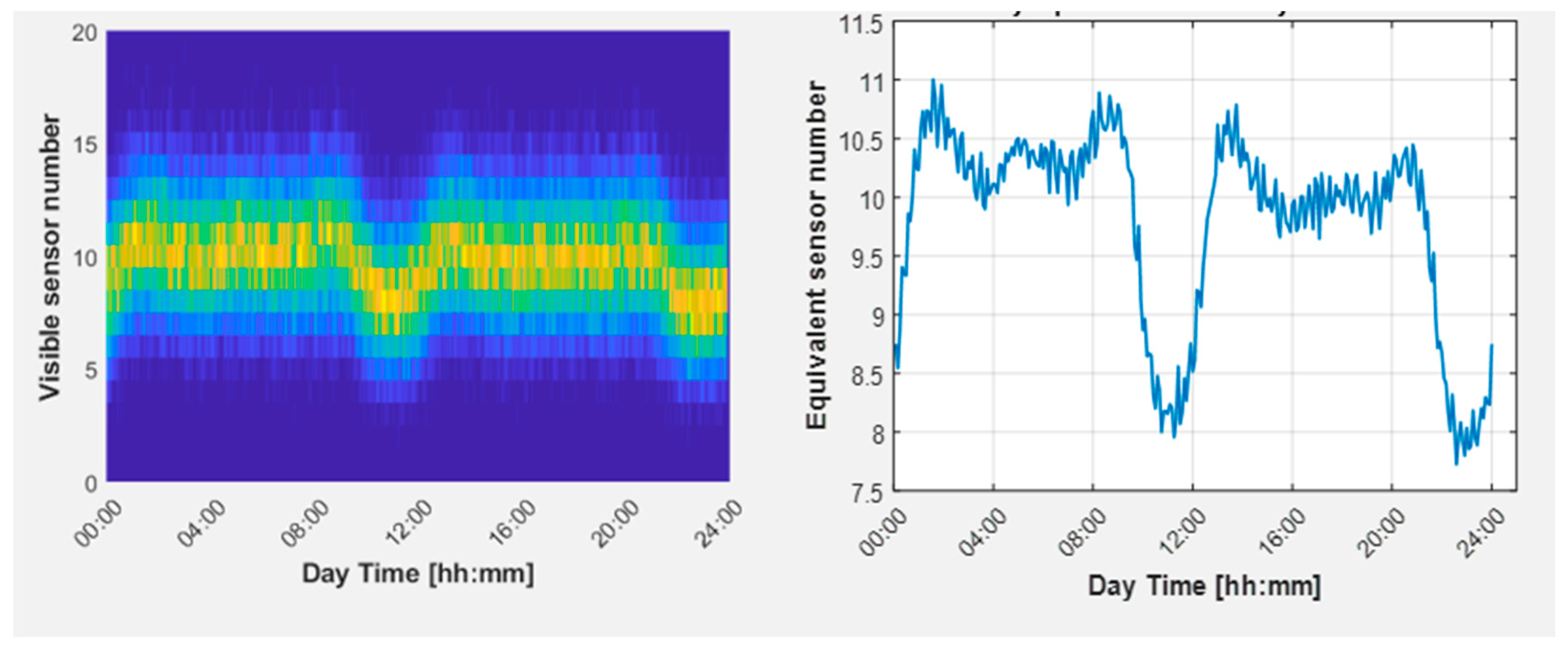
3.1. Mean Number of Satellites

The histogram of visibility with time, and the consequent mean number of satellites, plotted in Figure 6, confirms the daily periodic trend that is at the base of our choice to evaluate (3), with an average number that is roughly 1/3 of the satellites.

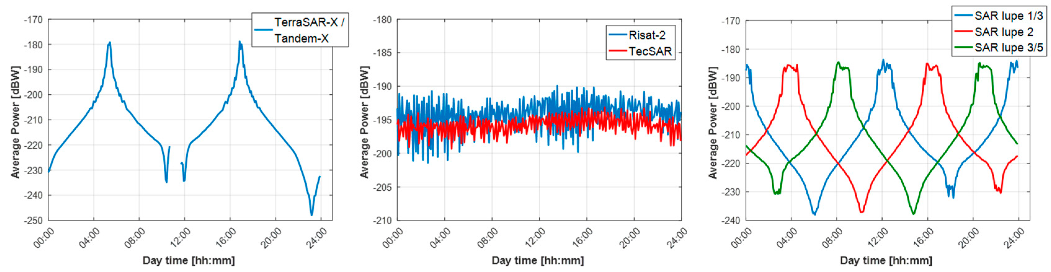
3.2. LEO Sensor Daily RFI Power

The daily distribution of RFI power is the information complementary to the mean number of satellites, used in (3) To express the mean power. In Table 1 we have classified three types of orbits: Sun synchronous (SS), dawn dusk, DD, and all the others. The DD is a special case of the SS orbit, whereby the LEO-SAR rides the terminator between day and night. In such conditions, solar panels can always see the Sun, without being shadowed by the Earth. This simplifies the Radar payload thermal design, and minimizes the power needed from batteries. Therefore, DD is the orbit chosen by many LEO-SAR, particularly those using high powers and high orbit duty cycle, that are likely to be those most disturbing to GEO-SAR (Figure 5).

In order to appreciate the contributions of the three different orbits, we have represented in Figure 6 the daily RFI for the DD, the SS, and the generic non-SS missions. Noticeably, all DD LEO-SARs interferences are concentrated in two timeslots during the 24 h, of which hours depends on the GEO-SAR longitudes. In addition, for SS satellites the interferences are concentrated on precise time slots, but different for each satellite. Finally, the non-SS missions, that have near-equatorial orbit, contribute with an approximately uniform disturbance, yet of minor extent.

In the RFI plotted in Figure 6 left and right, a sharp peak was removed by nulling about 10 s of acquisitions, where LEO-SAR illumination intersected the main lobe of GEO-SAR antenna beam. Such an interval is a minimal loss of data compared to the long GEO-SAR integration time, typically hours.

3.3. Total RFI Power

The resulting hourly scenario of total RFI power from the 30 LEO satellites listed in Table 1, as seen by a GEO-SAR placed at 10° E longitude, is plotted in Figure 7. This result can be interpreted as the product between the mean number of sensors, as shown in Figure 5, and the weighted average of RFI like those in Figure 6. Quite noticeable is the time-variation of the disturbances, with a dynamic of 18 dB, that confirm the usefulness of our daily estimate.

4. Performance Evaluation and Future Trend

The interference of LEO-SAR would depend on the GEO-SAR parameters in terms of antenna, power, and scene center, but also on the hour of the day in which GEO-SAR acquires, and the image time. Here we evaluate performance by assuming the GEO-SAR parameters as from

Table 2. Parameters for the X-band GEO-SAR.

Symbol	Definition	Value
λ	wavelength	3 cm
AG0	antenna equiv. area	20 m2
RG	range	37,000 km
BG	bandwidth	7.5 MHz
θG	incidence angle	50°
PG	mean tx power	400 W
	beam center (lat, long)	42°N, 10°E
ψ0	mean longitude	10°E

.

The noise equivalent sigma zero (NESZ) can be computed by equating the GEO and LEO power (1), (2) and integrating in the image time, Δ_t:

$${\sigma }_Z^0=\frac{1}{{\Delta }_t}{{\displaystyle \int }}_{t_0}^{t_0+{\Delta }_t}\overline{v}\left(t\right)·\overline{r}·\overline{d}·\frac{{\overline{P}}_T}{P_{TG}}·\frac{\overline{{\sigma }^0}\left(t\right)}{{\sigma }_G^0}·\frac{R_G^2}{\overline{R_G^2}\left(t\right)}·\frac{{\overline{G}}_G\left(t\right)}{G_{G0}}dt$$

(4)

and adding the thermal noise contribution [2,4,5,6].

The NESZ is reported in Figure 8 on the left, as function of the synthetic aperture and the time of the day. We notice the two red bands where NESZ achieves very bad values, up to 5 dB, preventing imaging for up to three hours in a day. However, for the rest of the time, acceptable values in the range from –14 to –22 dB are achieved. Furthermore, the expected variation of NESZ due to variation in the number of satellites has been plotted in Figure 8 On the right. This allows a prediction of GEO-SAR performance in the future, under the assumption that the time-averaged values in (3) will not change too much.

5. Mitigation

The mitigation strategies for RFI can be based either on coordination, or diversity in space, frequency, Doppler, code or time domains, or a mixture of all these [8].

The space domain mitigation is suggested after Figure 4: one should choose the GEO-SAR longitude so that the regions on the Earth, in yellow, where GEO-SAR is mostly sensitive to LEO-SAR backscatter are not frequently imaged by LEO-SARs, which may be those in open ocean.

The frequency domain mitigation is already accounted for by the term r_i in (3) A fine-tuning needs knowledge of LEO-SAR frequency usage, that could be done by on-ground measures.

As for Doppler domain, it is easy to show that, for distributed targets, no separation is possible since LEO-SAR backscatter observed by GEO-SAR is white, then sample-to-sample independent. Let us evaluate the LEO-to-GEO bistatic Doppler of target P:

$$\begin{gathered} f_{LE{O}_{GEO}}\left(t\right)=\frac{1}{\lambda }\frac{\partial R_b\left(P\right)}{\partial t}=\frac{1}{\lambda }\frac{\partial }{\partial t}\left(\left|S_{LEO}\left(t\right)-P\right|+\left|S_{GEO}\left(t\right)-P\right|\right)\simeq \frac{1}{\lambda }\frac{\partial }{\partial t}\left(\left|S_{LEO}\left(t\right)-P\right|\right) \\ =\frac{f_{LEO}\left(t\right)}{2} \end{gathered}$$

(5)

where the bistatic range, R_b, has been computed by assuming that the GEO-SAR position, S_GEO, does not change appreciably with time when compared with the LEO-SAR one, S_LEO(t). Then, the total Doppler bandwidth is half of the LEO-SAR monostatic:

$$B_{LE{O}_{GEO}}=\frac{B_{LEO}}{2}=\frac{v}{L_{LEO}}$$

(6)

This results in $B_{LE{O}_{GEO}}=700-7000$ Hz for a LEO-SAR with antenna length in the range of 1–10 m, whereas the pulse repetition frequency (PRF) of a typical GEO-SAR is at most 350 Hz for 400 km ground coverage [6]. Then, GEO-SAR always under-samples the bistatic backscatter from LEO-SAR, that would result in purely white process, making it indistinguishable from thermal noise.

While any separation in Doppler or even code domain would fail for distributed targets, the case of backscatter from isolated point targets is rather different. It is quite reasonable to assume that the pulse transmitted by LEO-SAR would be totally defocused when demodulated with a maybe different central frequency phase (also considering the different clocks) and correlated with a different pulse. Therefore, we have not to worry too much about the peak RFI, but only its mean value.

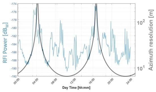
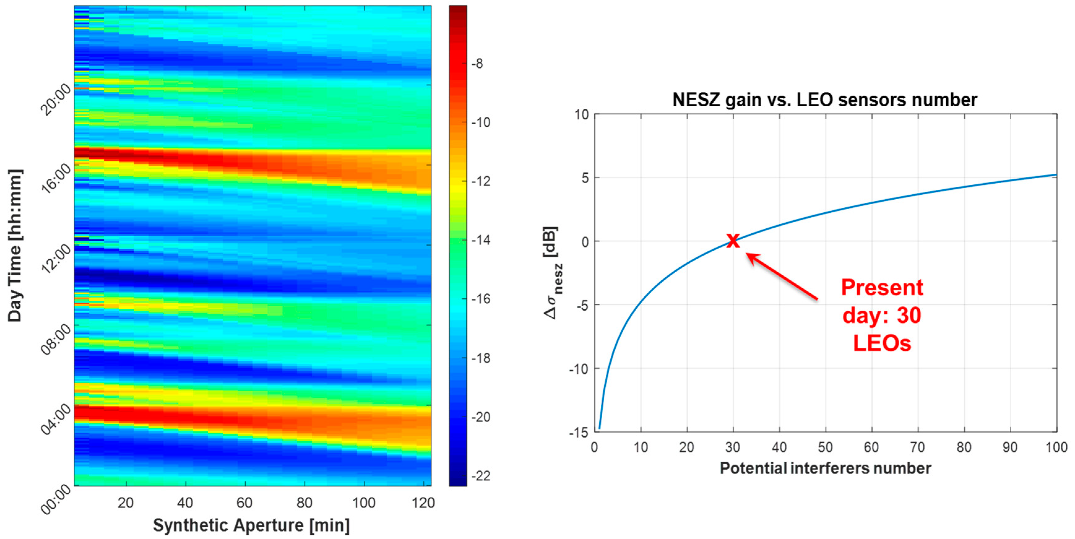
The time domain mitigation is the one suggested by our approach, and noticeable in Figure 8. The figure shows that there are two intervals over 24 h when NESZ is very bad. However, the GEO-SAR orbit is such that there are also two intervals when no imaging can be performed. Therefore, the best solution would be to match those intervals. To better understand how it can be done, let us evaluate the resolution achievable by a sub-aperture ΔTs, at different hours of the day. The GEO orbit in the Earth fixed frame is approximately an ellipse in the equatorial plane that can be expressed in polar format, as in [5]:

$$r_G\left(t\right)=R_g$$

(7)

$${\psi }_G\left(t\right)={\psi }_0+2e·sin\left({\mathsf{\Omega }}_E\left(t-t_p\right)\right)$$

where e is the eccentricity, Ω_E = 2π/86,400 the Earth angular speed, t_p the time the satellite crosses the perigee and ψ₀ the GEO-SAR longitude. The achievable synthetic aperture in an interval ΔTs can be approximated, for short intervals, as, where the instantaneous velocity is:

$$v=\frac{\partial }{\partial t}{R}_g·\psi \left(t\right)=2e·R_g·{\mathsf{\Omega }}_E·sin\left({\mathsf{\Omega }}_E\left(t-t_p\right)\right)$$

(8)

The GEO-SAR resolution is then computed for each time of the day, t, as:

$${\rho }_{az}=\frac{\lambda }{2L_s}=\frac{\lambda }{2v\Delta T_s}=\frac{\lambda }{4e·R_g·{\mathsf{\Omega }}_E·sin\left({\mathsf{\Omega }}_E\left(t-t_p\right)\right)·\Delta T_s}$$

(9)

and plotted in Figure 9 or different times since the perigee pass, t_p, and different sub-apertures. We assumed an eccentricity e < 0.002, the maximum allowed by ITU for geostationary satellites [14], then Figure 9 plots the best resolution available in X band. Notice that the resolution diverges for $t=t_p+N·12$ h (N integer), which corresponds to the stationary points in the orbit where v = 0 in (8).

The natural mitigation of RFI would then be to synchronize the perigee time, when no imaging is possible, see Figure 9, with the passage of DD LEO-SAR below the GEO-SAR, as suggested by Figure 8 and in the graphical abstract of this paper. This would improve the NESZ from 5 to less than 15 dB.

As a final remark, we notice that as bistatic backscatter in the end behaves like white noise, an additional mitigation, on the top of those so far discussed, is achieved just by increasing the integration time. This would be equally effective for any noise source. However, is does not appear by looking at NESZ profiles in Figure 8 (left). In fact, for a GEO-SAR the noise improvement provided by longer integration is perfectly balanced by the reduced signal that results from the better resolution [6]. Eventually one could trade the resolution to increase the number of looks, and then both the interferometric and radiometric quality.

6. Discussions

The 43× longer distance from Earth of GEO-SAR in respect to a LEO impacts in two destructive ways: (1) the power density on the ground is 42² = 1600 times lower at same antenna size, due to the bigger swath, and (2) the GEO-SAR antenna has poor directivity since the whole Earth is seen under a very small angle, just 19°. This means that RFI from LEO-SAR may be a potential killer for the mission. In fact, we see that in the present condition the RFI that is mostly driving the NESZ, and not the thermal noise.

The benefit and innovation of this paper is to underline two elements: (1) a proper backscatter model, that accounts for the almost orthogonal planes between illumination (from LEO-SAR) and backscatter (to GEO-SAR), and (2) the periodic illumination provided by dawn-dusk SAR, currently the majority. Both results in non-stationarity of the disturbances, respectively in space and time, and can be exploited to mitigate the impact of interferences.

It is suggested that the orbit longitude and time to perigee should be critically designed to minimize the RFI impact.

This analysis has been conducted with information about the present LEO-SAR scenario taken from public available sources and by filling many incomplete data. The real scenario could be quite different. However, this paper is intended as a framework where more precise information, maybe by on-ground measures, could be provided to get better predictions.

The theory exposed here is useful when most of the disturbances come from DD satellites, that are time synchronized and polar orbiting, and therefore causing scattering on the orthogonal plane. Conversely, it is totally useless for near equatorial-orbiting satellites. In the present scenario, there are seven non SS LEO-SAR (RISAT-2, TecSAR, Topaz1), over a total of 30, moreover, their mean backscatter was 5 dB lower that the other SS satellites. This seems to support the present framework.

7. Conclusions

The paper proposed a statistical model to evaluate the impact of the signal scattered from LEO-SAR illumination in the direction of a geostationary SAR. The analysis is carried out on an hourly basis, taking into consideration both the daily cycle of both GEO-SAR and sun synchronous satellites. Performance has been estimated by assuming an X band system, and the present scenario of 30 LEO-SARs. Statistics were evaluated by a computer simulation that averaged the interference from many orbits. The analyses show a dynamic range of 17 dB in noise equivalent sigma zero, depending on the hour of the day and the image time. This result, mostly due to the prevalence of dawn-dusk satellites, suggests an efficient mitigation that is implemented by synchronizing the GEO-SAR orbit with the DD passage, whereby other mitigation strategies have been analyzed.

The model is suited to be extended to future scenarios with different numbers of satellites, thanks to the statistics computed based on the present scenario.