Article

Upscaling Gross Primary Production in Corn-Soybean Rotation Systems in the Midwest

1
USDA-ARS, National Laboratory for Agriculture and the Environment, Ames, IA 50011, USA
2
USDA-ARS, Hydrology and Remote Sensing Laboratory, BARC-West, Beltsville, MD 20705, USA
3
Department of Food, Agricultural and Biological Engineering, The Ohio State University, Columbus, OH 43210, USA
*
Author to whom correspondence should be addressed.
Remote Sens. 2019, 11(14), 1688; https://doi.org/10.3390/rs11141688
Submission received: 29 May 2019 / Revised: 12 July 2019 / Accepted: 13 July 2019 / Published: 17 July 2019
(This article belongs to the Section Biogeosciences Remote Sensing)

Abstract

:
The Midwestern US is dominated by corn (Zea mays L.) and soybean (Glycine max [L.] Merr.) production, and the carbon dynamics of this region are dominated by these production systems. An accurate regional estimate of gross primary production (GPP) is imperative and requires upscaling approaches. The aim of this study was to upscale corn and soybean GPP (referred to as GPPcalc) in four counties in Central Iowa in the 2016 growing season (DOY 145–269). Eight eddy-covariance (EC) stations recorded carbon dioxide fluxes of corn (n = 4) and soybean (n = 4), and net ecosystem production (NEP) was partitioned into GPP and ecosystem respiration (RE). Additional field-measured NDVI was used to calculate radiation use efficiency (RUEmax). GPPcalc was calculated using 16 MODIS satellite images, ground-based RUEmax and meteorological data, and improved land use maps. Seasonal NEP, GPP, and RE ( x ¯ ± SE) were 678 ± 63, 1483 ± 100, and −805 ± 40 g C m−2 for corn, and 263 ± 40, 811 ± 53, and −548 ± 14 g C m−2 for soybean, respectively. Field-measured NDVI aligned well with MODIS fPAR (R2 = 0.99), and the calculated RUEmax was 3.24 and 1.90 g C MJ−1 for corn and soybean, respectively. The GPPcalc vs. EC-derived GPP had a RMSE of 2.24 and 2.81 g C m−2 d−1, for corn and soybean, respectively, which is an improvement to the GPPMODIS product (2.44 and 3.30 g C m−2 d−1, respectively). Corn yield, calculated from GPPcalc (12.82 ± 0.65 Mg ha−1), corresponded well to official yield data (13.09 ± 0.09 Mg ha−1), while soybean yield was overestimated (6.73 ± 0.27 vs. 4.03 ± 0.04 Mg ha−1). The approach presented has the potential to increase the accuracy of regional corn and soybean GPP and grain yield estimates by integrating field-based flux estimates with remote sensing reflectance observations and high-resolution land use maps.

1. Introduction

Midwestern US agriculture is dominated by corn (Zea mays L.) and soybean (Glycine max [L.] Merr.) production and both crops are important export commodities. In 2017, corn and soybean production in the United States made up 33% and 34% of total world production, and 56% and 46% of US production came from the Corn Belt states (Iowa, Nebraska, Indiana, Illinois, and Kansas), respectively [1,2]. Vast agricultural areas are used in the production of these crops which can impact gross primary production (GPP) and the global carbon cycle. The Midwestern US region was found to have one of the highest GPP rates in the northern hemisphere, owing to the large-scale production of corn, a C4 crop [3]. In addition, conventional corn and soybean production with bare soil in the off-season and frequent tillage events can impact GPP compared to reduced till systems [4]. Despite recent improvements in crop and soil management, no-till and cover crop systems only make up 35% and 4% in Iowa in 2017, respectively, meaning that conventional systems are prevailing [5]. Due to the economic and ecological importance of this region, the quantification of regional GPP as a proxy for yield as well as an essential part of the carbon cycle, remains imperative. The improvement of GPP estimations on a regional scale may also help to assess how changes in crop and soil management impact GPP and yield over time and may be used as decision support tool for climate-smart agriculture and best-practice management in terms of carbon cycling, soil quality, and crop performance.
There have been different approaches to quantify GPP from satellite images, such as the MODerate resolution Imaging Spectroradiometer (MODIS) satellite GPP product (MOD17A2) (referred to as GPPMODIS); however, the accuracy of these estimates has been limited to a regional scale [6,7]. Therefore, there have been different approaches proposed to improve the GPPMODIS estimate. MODIS products have been included in a biophysical model to calculate GPP on a global level, which showed good agreement to eddy covariance (EC) derived GPP [8,9]. Another modelling approach using MODIS imagery products could also improve GPP measurements in a Douglas fir stand [10]. Other models have been proposed in literature to ameliorate GPPMODIS [11]. A more parsimonious approach is the improvement of the maximum radiation use efficiency (RUEmax) and the fraction of absorbed photosynthetic active radiation (fPAR) estimates with field measurements and EC-derived GPP, as well as the use of land use maps [12,13,14,15]. In an analysis of GPPMODIS for Africa, it was stated that the MODIS biome parameters need further improvement [16]. This is also true for other biomes worldwide [17]. Accordingly, new input parameters were used to up-scale GPP from field to whole regions in the Midwestern US using MODIS products [12,13]. However, previous studies in the Midwestern US were either constrained by the density of ground-based EC stations (i.e., number of EC stations per area), or by the lack of field-based measurements of RUEmax or fPAR [12,13]. In addition, new land use maps were developed to distinguish crop fields with higher accuracy [18]. The aim of this study was to up-scale GPP with MODIS satellite image products from field to county using eight EC stations distributed across four counties in Iowa, additional field-based canopy reflectance measurements, and improved land use maps for the growing season of 2016. Therefore, crop-specific RUEmax were calculated, and GPP products evaluated.

2. Material and Methods
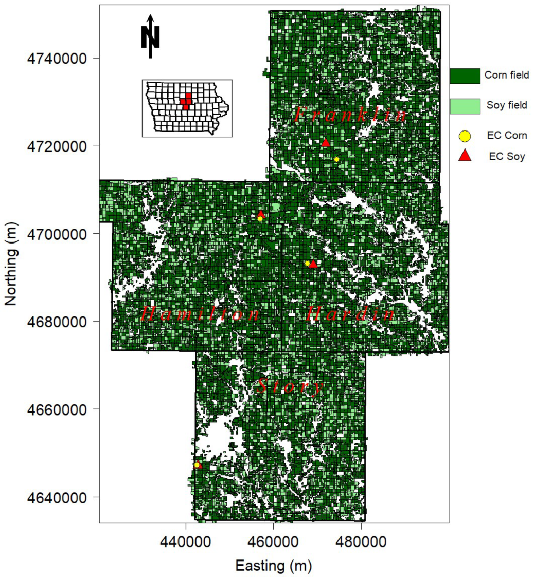
2.1. Study Sites

The study was conducted as part of the Soil Moisture Active Passive Validation Experiment in 2016 (SMAPVEX16) during the growing season (i.e., day of year (DOY) 145–269; total: 125 days) in four neighboring counties in North Central Iowa: Story, Franklin, Hamilton, and Hardin County [19,20]. The overall experiment was dedicated to exploring the land surface soil moisture conditions across a homogeneous landscape to improve vegetation characterization and soil moisture remote sensing algorithms via the Soil Moisture Active Passive Mission. Within each county, two field sites under a corn-soybean rotation, one each planted in corn and the other in soybeans (Figure 1). The sites are located on the Des Moines Lobe and soils belong to the Clarion-Nicollet-Webster association [21]. The site characteristics are summarized in Table 1. The sites reflect well the dominating crop and soil management conditions of the four counties, with 98% of the harvested cropland used for corn and soybean production, and only 13% of the cropped area under no-till and 3% planted with cover crops [5]. In terms of climatic parameters, the 30-year (1986–2016) minimum and maximum temperature between June and September averaged (± SE) over four nearby weather stations was 15.38 ± 0.16 and 26.94 ± 0.08 °C. All agricultural sites are rain-fed systems with a seasonal 30-year precipitation of 508 ± 17 mm [22].

2.2. Eddy Covariance Datasets

Turbulent fluxes of carbon dioxide (Fc) were computed at each site (n = 8 EC stations) using the EC method [23]. One EC station was deployed in each field, so that the EC footprint covered the crop of interest in a representative portion of the field and in the main wind direction. The 90% footprint of each EC station was calculated [24], and mean (± SD) flux footprint area was 4.4 ± 2.3 ha (Figure A1). The 90% footprint area at the corn-site in Franklin County surpassed the field, and the footprint was cropped to field boundaries. Note that most of the information recorded by the sensor is from nearby the EC station and not from the edges of the footprint. Also, the footprint area is an average of the entire season including day- and nighttime data, with higher fetch during night than during the day. An open-path infrared gas analyzer (IRGA) measured carbon dioxide and water density. Instantaneous high frequency sonic temperature and wind speed velocity components were measured with a 3-D sonic anemometer. The measurement height of IRGAs and sonic anemometers ranged between 200 and 500 cm, depending on crop height during the season. The Fc were computed as the covariance between the instantaneous vertical wind velocity and carbon dioxide density. The Fc was coordinate rotated [25] and corrected for temperature and air density variations [26]. The EC sampling rate (high frequency) was 20 Hz and was averaged to a 15-min time interval. Sonic and IRGA models and manufacturers are presented in Table 1.
A net radiometer measured incoming shortwave radiation (Table 1). An air temperature and humidity probe measured ambient air temperature (Ta) and relative humidity (rH) (Vaisala HMP45c, Vantaa, Finland). Precipitation was recorded using tipping bucket rain gauges (Model TR525 USW, Texas Electronics, Dallas, TX, USA). Soil moisture content was measured at 10 cm depth with soil moisture probes (Hydra Probe, Stevens Water Monitoring Systems, Portland, OR, USA). Thermocouples were buried at 2 and 6 cm to measure soil temperature, and heat flux plates (HFT-1, Radiation Energy Balance, Seattle, WA, USA) measured soil heat flux at 6 cm soil depth. An infrared temperature sensor (IRR, Apogee Instruments Inc., Logan, UT, USA) measured surface temperature and mounted at 45° from perpendicular. The ancillary instrumentation was sampled at 0.1 Hz and averaged on a 15-min interval. The data were recorded on data loggers (CR5000, Campbell Scientific, Logan, UT). Further specifications of the EC systems are listed in Table 1.

2.3. Outlier Detection and Interpolation

The EC data were screened for statistical outliers and sensor failures and thereafter interpolated to fill data gaps [27]. Data was excluded under unfavorable weather conditions, such as during rain events, low wind turbulence and wind directions opposite to the sonic sensor direction [28], and time periods with high rH [29]. The internal sonic and IRGA warning flags and automated gain control were used to identify low-quality data. Data were screened for outliers using empirical set limits and the interquartile range (IQR) procedure, where outliers were defined as 1st/3rd Quartile ± 3.5 * IQR. Then the data were interpolated with an inverse weighted time average procedure [30]. The Fc was separated for day- and nighttime (Fc day, Fc night) and Fc night (i.e., nighttime respiration) was interpolated using the relationship between air temperature and CO2 fluxes [31], while Fc day was gap filled with daily light response curves [32]. Approximately 31%–55% of the 15-min Fc data was excluded, and Fc night was more affected than Fc day. Approximately 29%–42% of the Fc data was interpolated. Daily values were calculated as the daily average multiplied by the number of samples per day.
Daily net ecosystem production (NEP) was calculated as the sum of daily Fc day and Fc night. Here the arithmetic sign convention is positive for Fc from the atmosphere to the surface. The NEP was partitioned into GPP and RE. The GPP was calculated as the difference between NEP and RE. Daily RE was calculated as the sum of Fc night and daytime respiration (Rd). Rd was derived from the non-linear relationship between incoming photosynthetic active radiation (IPAR) and Fc day using light response curves, such as the rectangular hyperbola function [32]:
F c   d a y   =   A Q Y I P A R   P g   m a x     P g   m a x + A Q Y I P A R   R d
where: Fc day = daytime CO2 flux (μmol m−2 s−1); AQY = apparent quantum yield (μmol CO2 μmol PAR−1), Pg max = maximum gross photosynthesis rate (μmol CO2 m−2 s−1); IPAR = photosynthetic active radiation (μmol m−2 s−1); Rd = mean daytime respiration (μmol CO2 m−2 s−1).
IPAR was assumed to be 45% of incoming shortwave radiation [5] and was converted to photon flux density with 1 W m−2 = 4.6 μmol m−2 s−1 [33].
Daily NEP, RE, GPP and Rd values were screened again for outliers and interpolated using the inverse weighted time average procedure. Seasonal values were calculated as seasonal averages multiplied with number of days.

2.4. NDVI Ground-Based Measurements

Reflectance data on the ground were measured with a radiometer (CropScan, CROPSCAN, Inc., Rochester, MN, USA) in the corn and soybean field in Story County during the 2016 growing season. A total of 33 and 31 measurements were made on soybean and corn, respectively, in observation intervals of 2–14 days between DOY 124 and 308. Measurements were constrained to clear-sky conditions or with little cirrus clouds and with sun angles > 45° (i.e., 10.00 and 14.00 CST). The radiometer measured reflected and incoming radiation at 16 wavebands between 460 and 1700 nm. Each measurement consisted of 30 individual scans, and an average is calculated by the unit. Measurements were taken above the crop at five locations north of the EC stations, and the measurement height was adjusted to yield a surface pixel size of 1.5 m. The radiometer was calibrated with a reflectance panel and a dark measurement prior to field observations. The Normalized Difference Vegetation Index (NDVI) was calculated as:
N D V I =   ρ 760     ρ 660 ρ 760 +   ρ 660
where: ρ660 and ρ760 were the surface reflectance of the red (660 nm) and near-infrared (760 nm) wavelength bands, respectively.
The individual observations at each location were averaged, and the averaged values interpolated with an inverse weighted time average procedure to yield a daily NDVI dataset for the 2016 growing season. Further information on CropScan measurements can be found in literature [34,35]. In addition to NDVI measurement, plant development and plant height was recorded (corn n = 21, soybean n = 40). The development stages are categorized in vegetative and reproductive growth as V and R Stages, respectively. The V-Stages in corn categorize plant emergence (VE), number of fully developed leaves (e.g., V1 for first leaf) and tasseling (VT), while the six R-Stages categorize corn flowering (R1), and ear development (R2-5) until maturation and senescence (R6) [36]. The V-stages in soybean categorize plant emergence (VE), first unifoliate leaf (VC), and number of fully developed trifoliate leaves on the main stem. In contrast to corn, reproductive stages occur during plant growth (V-stages), and categorize flowering (R1-2), pod development (R3-6), and maturation and senescence (R7-8) [37]. Plant height was measured from the ground to the top of the canopy, and daily height was calculated by fitting a three-parameter sigmoidal model. Due to resource restrictions, NDVI and intensive crop measurements were limited to the site in Story County.

2.5. MODIS fPAR Products, and Land Use Maps

The fraction of absorbed IPAR (400–700 nm wavelength), fPAR, can be derived from MODIS satellite images, and MODIS fPAR products (MCD15A2H) were provided by the U.S. Geological Survey [38,39]. The MODIS fPAR product had a resolution of 500 × 500 m and images are available at an 8-day interval. In total, 16 fPAR scenes between DOY 145 and 265 for the North Central Iowa counties were obtained. The quality of the fPAR scenes was checked with the Q/C layers provided by USGS, and areas of low quality were excluded.
The fPAR scenes were cropped to the 90% footprint area (i.e., two to four data points) of each EC station, as well as for the corn and soybean fields in each county. Corn and soybean fields were identified using the 2016 county land use maps (Figure 1) provided by the Agricultural Conservation Planning Framework (ACPF) [18]. Only fields with a land use area >55% designated for corn and soybean production were used.

2.6. GPP Upscaling and Radiation Use Efficiency

The 8-day GPPMODIS product from MODIS satellite imagery (MOD17A2H) is calculated as [6]:
G P P M O D I S = R U E m a x T m i n s V P D s f P A R I P A R
where: GPPMODIS = MODIS gross primary production product (g C m−2 8-day−1), RUEmax = maximum radiation use efficiency (g C MJ−1), Tmins = a temperature scalar (no units), VPDs = a vapor pressure deficit scalar (no units), fPAR = fraction of IPAR absorbed by the crop (no units), IPAR = incoming photosynthetic active radiation (MJ m−2 d−1).
Note that the GPPMODIS is calculated as 8-day sums, and daily values can only be calculated as daily means (Appendix B). The scalars Tmins and VPDs are proxies for RUEmax limitations of temperature and vapor pressure deficit (VPD), respectively. The scalars Tmins and VPDs are calculated as [6]:
T m i n s = { 0 T m i n <   T l i m m i n T m i n T l i m m i n T l i m m a x   T l i m m i n T l i m m i n   T m i n   T l i m m a x 1 T m i n >   T l i m m a x
V P D s   { 0 V P D > V P D m a x 1 V P D V P D m i n V P D m a x   V P D m i n V P D m i n V P D V P D m s x 1 V P D < V P D m i n
where: Tmins = scalar for daily Tmin (no units), Tmin = daily minimum Ta (°C), Tlimmin = lower Tmin limit (°C), Tlimmax = upper Tmin limit (°C), VPDs = scalar for daytime VPD (no units), VPD = average daytime vapor pressure deficit (kPa), VPDmin = lower VPD limit (kPa), VPDmax = upper VPD limit (kPa).
The Tlimmin and Tlimmax are set to −8 and 12.02°C, while VPDmin and VPDmax are set to 0.65 and 4.3 kPa, respectively [6].
The GPP was upscaled from field to county following the same concept in Equation (3) (referred to as GPPcalc). First, RUEmax for corn and soybean was calculated using the EC station data and NDVI field measurements from the Story County site. Equation (3) was solved for RUEmax and fPAR substituted with field-measured corn and soybean NDVI, assuming that fPAR ≈ NDVI [6]. The VPD was calculated as the difference between saturated (es) and actual vapor pressure (ea), of which the former was calculated as a function of Ta [40], and the latter as es multiplied with rH. Then VPDs and Tlims were calculated. RUEmax was calculated as the slope of a linear regression (p < 0.05) with the product of Tlims, VPDs, NDVI and IPAR as independent variable and EC-derived GPP as dependent variable [7]. At last, GPPcalc was upscaled for the whole county using Equation (3), with MODIS fPAR products cropped for county-wide corn and soybean fields, respectively, and crop-specific RUEmax. GPPcalc was set to zero when fPAR < 0.4 (see Section 4).

2.7. Data Preparation, and Statistical Analysis

The variation of corn and soybean GPP among EC stations was quantified by calculating the 95% confidence intervals (CI) using the bootstrap percentile method with two thousand replications. Bootstrapping was run with the boot package in R [41]. Relationships between NEP, GPP, RE and climate parameters were evaluated with Pearson correlation and the regression coefficient (r) was calculated. The ACPF land use maps were validated with the 2016 county-wide corn and soybean production area [1] using linear regression analysis (p < 0.05) and cross-checked with the MODIS land cover type product (MCD12Q1) from 2016 [38,42]. The median EC-footprint and county-wide fPAR, GPPcalc, and GPPMODIS were calculated for further analysis. The footprint fPAR was validated against field-measured NDVI with linear regression analysis (p < 0.05). GPPcalc was validated against EC-derived GPP using a linear regression analysis (p < 0.05) and was also compared to the GPPMODIS product [5,38]. The median county-wide GPPcalc was interpolated with an inverse weighted time average procedure to produce a daily dataset, and grain yield was calculated [7,12] as:
Y i e l d G P P =   G P P c a l c H I ( 1 +   R S )   1 ( 1   M ) O C    
where: YieldGPP = calculated yield data (Mg dry weight ha−1), GPPcalc = seasonal sum of daily median county GPPcalc (g C m−2), HI = Harvest index, RS = root-shoot ratio, M = % moisture content, OC = % grain carbon content.
The HI was set to 0.50 and 0.57 [43,44], the RS was 0.18 and 0.15 [45], M was 15.5% and 13%, and OC was 44.7% and 54% [46], for corn and soybean, respectively. The YieldGPP was compared to the 2016 county yield data [1]. All figures were created with the R programming language [41].

3. Results

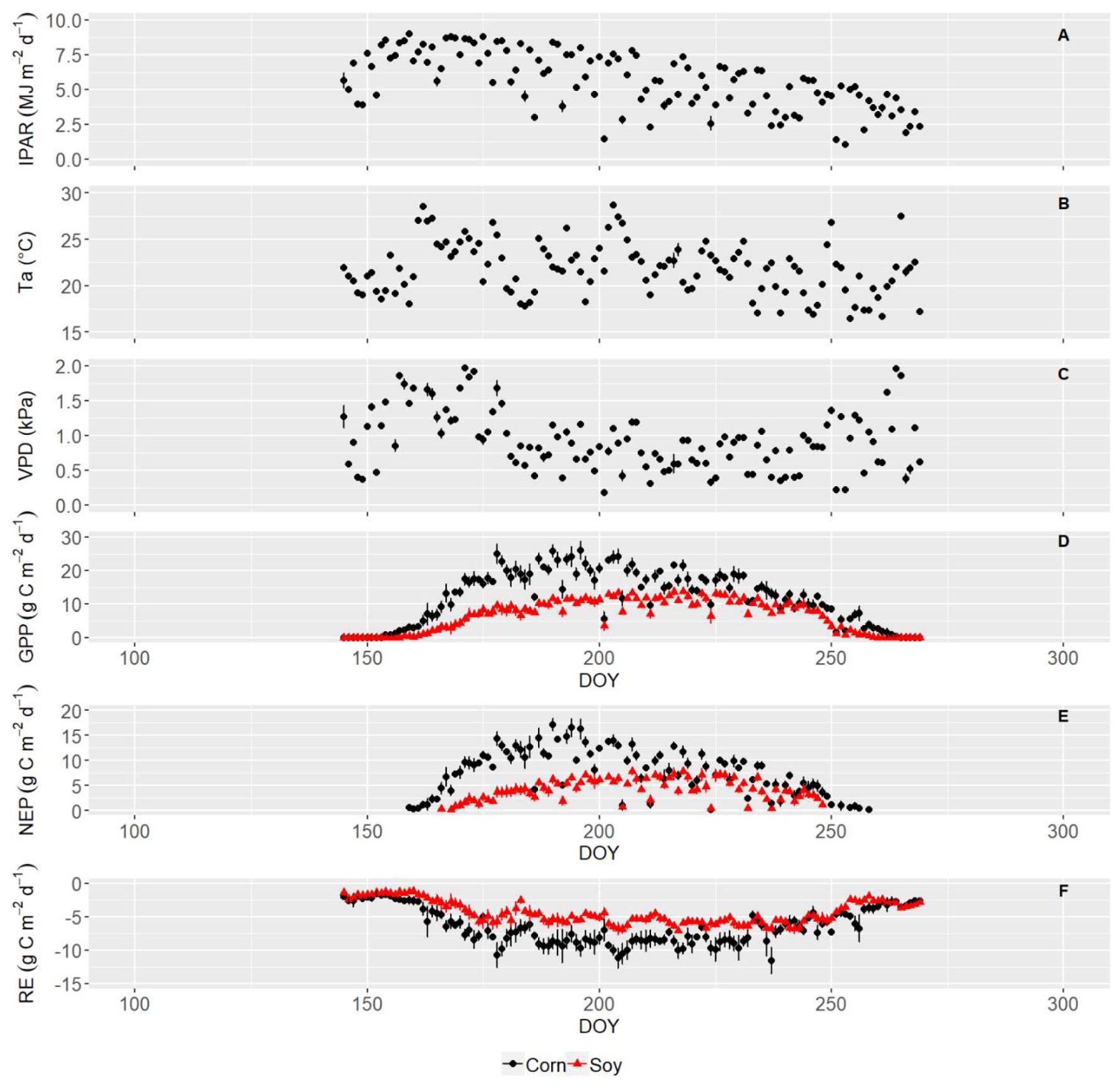
3.1. Eddy-Flux Station Data

Eight EC stations measured carbon fluxes and meteorological data in fields with corn-soybean rotation during the growing season 2016. Mean daily IPAR decreased from 8.98 MJ m−2 on DOY 159 to 1.02 MJ m−2 on DOY 253 (Figure 2A). Mean Ta ranged from 16.4 and 28.8 °C (Figure 2B) and mean (± SE) seasonal precipitation was 515 ± 51 mm, which is warmer and with near normal rainfall compared to the 30-year seasonal average (see Section 2.1). The average daytime VPD ranged between 0.13–2.40 kPa (Figure 2C).
Maximum average corn GPP (± SE) was reached at DOY 196 with 26.0 ± 3.2 g C m−2 d−1, and maximum average soybean GPP was reached at DOY 218 with 13.7 ± 2.3 g C m−2 d−1 (Figure 2D). Seasonal corn and soybean GPP were 1483 ± 100 and 811 ± 53 g C m−2, respectively (Table 2). Mean corn NEP ranged from −3.6 to 17.1 g C m−2 d−1 (Figure 2E), with a site-average (± SE) seasonal total of 678 ± 63 g C m−2 (Table 2). The 95% CI are presented in Table 2. Cumulative corn NEP was greater than zero (i.e., carbon uptake > respiration) starting from DOY 169. Mean soybean NEP ranged from −3.7 to 7.8 g C m−2 d−1 (Figure 2E), with a seasonal NEP of 263 ± 40 g C m−2 (Table 2). Cumulative seasonal soybean NEP surpassed zero from DOY 181. Minimum corn RE (i.e., highest respiration) was reached at DOY 204 with -11.6 g C m−2 d−1, and maximum corn RE at DOY 237 with -1.6 g C m−2 d−1 (Figure 2F). Minimum soybean RE was at DOY 160 with −7.1 g C m−2 d−1, and maximum soybean RE at DOY 217 with −1.2 g C m−2 d−1. Seasonal corn and soybean RE were −805 ± 40 and −548 ± 14 g C m−2, respectively (Table 2). NEP, RE, and GPP followed the seasonal and daily pattern of Ta, IPAR, and VPD (Figure 2). The site-specific daily NEP was weakly correlated to IPAR (r = 0.20–0.54), daytime VPD (r = 0.02–0.41), and Tmin (r = −0.01–0.21). Daily GPP was weakly correlated to IPAR (r = 0.11–0.45), daytime VPD (r = 0.02–0.47), and Tmin (r = 0.07–0.31) as well. Also, daily RE was weakly correlated to IPAR (r = −0.18–0.20), daytime VPD (r = 0.02–0.48), and Tmin (r = 0.22–0.42).

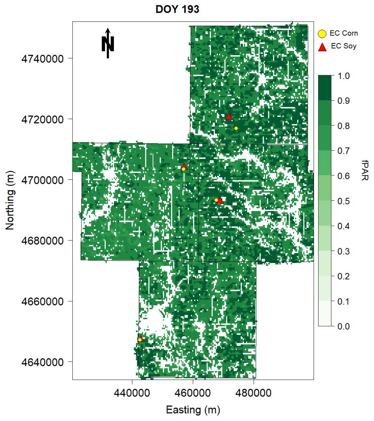
3.2. MODIS fPAR vs NDVI

The NDVI was measured in one corn and soybean field in Story County and compared to MODIS fPAR products. Field-measured daily corn and soybean NDVI ranged from 0.15–0.88 and from 0.16–0.91 (Figure 3A). Corn NDVI was < 0.4 until DOY 156 and after DOY 256, which corresponds to development stages V6 and R6. Soybean NDVI was < 0.4 until DOY 163 and after DOY 259, which corresponds to phenological stages V3 and V22/R7. Corn reached NDVI values > 0.75 early in the season at DOY 166, where plants reached phenological stage V8-9 with an average height of 0.95 m.
Soybean NDVI reached values > 0.75 later than corn at DOY 180, corresponding to plant development stage V8-10/R1-2 and an average height of approximately 0.40 m. There was a significant linear relationship (p < 0.05) between field-measured NDVI and MODIS fPAR within the 90% footprint area of the EC station, explaining 99% of the fPAR variation with a slope of 1.02 and 0.99 for corn and soybean, respectively (Figure 3B).
The RUEmax was then calculated with Equation (3), substituting fPAR with NDVI and using meteorological data and GPP from the EC stations in the studied corn and soybean field in Story County. The RUEmax was the slope of a linear regression with GPP as dependent and the product of Tmin, VPDmin, IPAR, and NDVI as independent variables. The derived daily corn and soybean RUEmax was 3.24 and 1.90 g C MJ−1. The linear relationship was significant at p < 0.05, explaining 93% and 89% of the GPP variation for corn and soybean, respectively (Figure 3C).

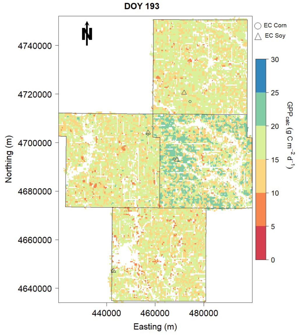
3.3. Upscaling GPP to County Level

The total corn and soybean area from the ACPF land use maps corresponded well with the official production area in 2016 [1] (y = 1.01x; R2 = 0.99, p < 0.05, n = 8). The land use maps also corresponded well with the MODIS land cover in 2016, and >99% of the ACPF map area used was classified as cropland in the MODIS land cover map. The average (± SE) ACPF land use area of corn and soybean in 2016 made up 55% ± 2% and 26% ± 1% of the total land area in four counties, respectively.
The average within-county fPAR range (difference between maximum and minimum fPAR) was 0.65 at DOY 145, decreased to 0.32 at DOY 201 and increased again to 0.65 at DOY 265 (Figure 4, Video S1). The county median fPAR ranged from 0.25–0.9 with little variation among crops and counties during the 2016 growing season (Figure 5A). Calculated daily corn and soybean GPP followed a seasonal pattern with highest values at 22.1 and 11.7 g C m−2 d−1, respectively (Figure 5B). A linear regression between EC-derived GPP and GPPcalc within the 90% footprint was significant at p < 0.05, with a coefficient of determination (R2) of 0.96 and 0.86 and a root mean square error (RMSE) of 2.24 and 2.81 g C m−2 d−1, for corn and soybean, respectively (Figure 5C). A linear regression between EC-derived GPP and daily GPPMODIS within the 90% footprint was significant at p < 0.05, with a R2 of 0.89 and 0.21 and a RMSE of 2.44 and 3.30 g C m−2 d−1 for corn and soybean, respectively. GPPMODIS was not substantially different between crops, overestimated GPP at the onset and end of the season, and underestimated corn GPP (Figure A2 and Figure A3).
The average within-county corn and soybean GPPcalc range (difference between maximum and minimum GPPcalc) was 13.2 and 6.0 g C m−2 d−1 at DOY 145, decreased to 1.5 and 0.9 g C m−2 d−1 at DOY 201 and increased again to 5.1 and 3.6 g C m−2 d−1 at DOY 265 (Figure 6). The YieldGPP was 12.82 ± 0.65 and 6.73 ± 0.27 Mg ha−1, for corn and soybean, respectively (Table 2). The official county-wide corn and soybean yield in 2016 was 13.09 ± 0.09 and 4.03 ± 0.04 Mg ha−1, respectively [1].

4. Discussion

In this study, the 2016 corn and soybean GPPcalc in four counties were upscaled using ground measurements of GPP, NDVI, and meteorological data as well as MODIS fPAR products. In contrast to previous studies, seasonal GPP, NEP, and RE from several EC stations concentrated on a relatively small land area were retrieved. It was therefore possible to estimate the spatial variation of GPP under similar climate conditions and for a relatively small land area as compared to previous studies [12,13,14,15]. The calculated 95% CI indicate a substantial variation in GPP, NEP, and RE among sites, despite that the studied fields are well represented in the four counties [5] and the relatively high density of EC stations used. Individual spatial variation in GPP is probably connected to climate, soil and crop management (Table 1, Table 2), such as precipitation, cloud cover, crop growth, crop varieties, fertilizer application, tillage, and amount of crop residues among others. Analyzing for these impacting factors was beyond the scope of this study and would require more information of each field but may be important to further increase the accuracy of GPPcalc. In a previous study, substantial variation in corn and soybean Fc and precipitation using 12 EC stations in a 5000-ha Midwestern US watershed was found, and this was accounted to difference in ground cover, plant growth and biomass accumulation among fields [47]. Differences in soil tillage has also impacted GPP [4], and soil respiration varies with nitrogen fertilizer application, irrigation, and tillage [48]. This indicates that a higher density of EC stations than typically used in field studies is needed to cover the spatial variation of GPPcalc. The higher NEP values in corn are connected to higher photosynthetic rates of corn as a C4 crop, compared to soybean as a C3 crop. In addition, high amounts of corn residues from the previous season remain in the soybean fields, which further decreases NEP due to higher residue mineralization [27].
The GPPcalc was more accurate than GPPMODIS, as evidenced by lower RMSE in comparison to EC-derived GPP. Field measurements of RUEmax, improved land use maps, and a higher resolution of IPAR, Ta, and VPD measurements increased the accuracy of GPPcalc compared to GPPMODIS.
One important tool to increase the accuracy of GPPcalc compared to GPPMODIS was the ACPF land use map [18], which enabled distinction between corn and soybean fields within each county. The ACPF land use maps are based on an ensemble of aerial photographs, satellite imagery, and other land use map products [18]. Earlier studies on corn and soybean production in the Midwestern US were constraint to the Cropland Data Layer (CDL) and an area-weighted, crop-specific value was used to estimate GPP contribution by crop [12,13]. To the best of our knowledge, this is the first time that ACPF land use maps have been used to upscale GPPcalc. The field boundaries provided by ACPF land use maps were the basis to create GPPcalc maps as separated by crop. Approximately, ¾ of the total land area in the studied counties were used for corn and soybean production, which demonstrates the economic importance and its impact on the carbon cycle in the region. There were more fields used for corn than for soybean production in the studied counties in 2016, and corn GPP (as a C4 crop) was higher than soybean GPP (as a C3 crop) (Figure 2D). Consequently, the tempo-spatial variation in corn and soybean fields determines the amount of county-wide, seasonal cropland GPPcalc. Accurate and annually updated land use maps are therefore imperative to upscale GPPcalc and is important to improve GPPMODIS.
Another significant parameter to improve GPPMODIS is a crop-specific RUEmax, which determines the maximum amount of GPP per unit of absorbed IPAR (i.e., fPAR × IPAR). Similar corn and soybean RUEmax of 3.17 and 1.91 g C MJ−1 had previously been reported using EC data and MODIS fPAR in corn and soybean fields in the Midwestern US [12]. For the GPPMODIS product the RUEmax is determined according to land cover categories (from MODIS MCD12Q1 land cover types), and a cropland RUEmax of 1.044 g C MJ−1 was proposed [6]. This is lower than the corn and soybean RUEmax in this study and does not distinguish between both crops. This consequently leads to the substantial underestimation of GPPMODIS, especially for corn as a C4 crop (Figure A2 and Figure A3, Video S2, Video S3).
The MODIS fPAR product within the EC footprint corresponded well with NDVI measurements on the ground for both crops, which is interesting considering the difference in resolution (i.e., 500 x 500 m satellite image vs. 1.5 m x 1.5 m pixel size of field measurement). It also indicates that MODIS fPAR displays the NDVI of both crops. It was also noted that Equation (3) overestimates GPPcalc at the beginning and the end of the growing season, where the EC-measured GPP was zero (Figure A2). This problem was somewhat resolved by setting GPPcalc to zero, when fPAR < 0.4 (i.e., early and late in plant development). A field-measured NDVI value of 0.15 was found for bare soil in corn and soybean, similar to this study [28], and GPP is zero. It is likely that NDVI and MODIS fPAR do not represent GPPcalc well in the early and late stages of plant development, despite that NDVI was found to be a good indicator of intercepted PAR [35]. A field-based fPAR as well as other MODIS imagery-derived VIs further improved GPPcalc in corn and soybeans [14,15].
The importance of RUEmax, fPAR, and land use maps should not diminish the importance of accurate meteorological data, as it determines the amount of energy intercepted by the crop (IPAR) and to what extent RUE is limited by temperature and VPD constraints (i.e., Tmins and VPDs scalars). This eventually determines the amount of GPPcalc. For example, on DOY 201, the median-county GPPcalc was low, because IPAR was low at all eight EC stations (Figure 2A and Figure 5B). Although the variation of IPAR, Ta, and VPD was low among EC stations (Figure 2), these variables impacted among-county daily GPPcalc variation. For example, corn GPPcalc on DOY 193 was higher in Hardin county owing to slightly higher VPDs and IPAR (Figure 6, Video S3). Political boundary delimitations (i.e., counties) are not connected to these climatic changes, and further methods are needed to model the spatial variation of IPAR, Ta, and VPD with higher resolution. Within-county variation of corn and soybean GPPcalc is therefore only driven by the MODIS fPAR products in this study. In this study, IPAR, Ta, and VPD from ground measurements were used because of the relatively high resolution among stations. However, this may not always be the case. For example, the global GPPMODIS product is calculated with meteorological data provided from the NCEP-DOE reanalysis II datasets, which have a coarser resolution than the density of EC stations used in this study [49].
The seasonal sum of county-median GPPcalc was used to estimate YieldGPP, which was compared to actual county yield data. While corn YieldGPP corresponded well with county corn yield in 2016, soybean YieldGPP was overestimated (Table 2). There has been good agreement between YieldGPP and actual yield values in corn and soybean [13], and wheat [7], however, both studies found limitations of the approach. YieldGPP as shown in Equation (6) depends on more factors (HI, M, OC, and RS may differ among fields) than GPPcalc and this estimation only represents a general trend. The overestimation of soybean YieldGPP could be connected to the mineralization of the 2015 corn residues in soybean-years in these corn-soybean rotation systems. The mineralization of corn residues from the previous growing season can have a substantial impact on current-year soybean NEP, GPP, and RE [4]; thus, the GPPcalc as combined value of corn residue respiration and soybean assimilation may underrepresent soybean yield.

5. Conclusions

It was shown in this study, that GPPcalc can be upscaled with higher accuracy (i.e., lower RMSE) than GPPMODIS. The GPPMODIS product does not distinguish among crops, which leads to a substantial underestimation of C4 crops such as corn. The fPAR MODIS product agreed with ground-measured NDVI. The meteorological data showed low variation among EC stations, indicating that a coarse-resolution meteorological dataset may be sufficient to upscale regional bulk GPP in this region of Iowa. However, variation of soil and crop management as well as micro-climate may require a higher density of EC and weather stations to estimate GPPcalc on a field level. A substantial improvement of upscaling regional GPP can be achieved using crop-specific RUEmax and improved land use maps. A more detailed categorization of MODIS land use maps (e.g., cropland C4 crops vs. cropland C3 crops), a crop-specific RUEmax, and a different VI for the beginning and end of the growing season can increase the accuracy of GPPMODIS without the need to modify the algorithm or substantial re-processing of imagery.

Supplementary Materials

The following are available online at https://www.mdpi.com/2072-4292/11/14/1688/s1, Video S1: MODIS fPAR, Video S2: GPPMODIS, Video S3: GPPcalc.

Author Contributions

For research articles with several authors, a short paragraph specifying their individual contributions must be provided. The following statements should be used “conceptualization, C.D., K.M.W. and J.H.P.; methodology, C.D., K.M.W., and J.H.P.; software, C.D. and J.H.P.; validation, C.D.; formal analysis, C.D. and J.H.P.; investigation, C.D. and J.H.P.; resources, J.L.H., J.H.P., T.B.M., T.J.S., M.H.C. and D.D.; data curation, C.D.; writing—original draft preparation, C.D.; writing—review and editing, C.D., K.M.W., J.L.H., J.H.P., T.B.M., T.J.S., M.H.C. and D.D.; visualization, C.D.; supervision, J.L.H. and J.H.P.; project administration, J.L.H., J.H.P., T.B.M., T.J.S., M.H.C. and D.D.; funding acquisition, JH, TM and TS”, please turn to the CRediT taxonomy for the term explanation. Authorship must be limited to those who have contributed substantially to the work reported.

Funding

This research was supported in part by an appointment to the Agricultural Research Service (ARS) Research Participation Program administered by the Oak Ridge Institute for Science and Education (ORISE) through an interagency agreement between the U.S. Department of Energy (DOE) and the U.S. Department of Agriculture (USDA). ORISE is managed by ORAU under DOE contract number DE-AC05-06OR23100. USDA is an equal opportunity provider and employer. All opinions expressed in this paper are the author’s and do not necessarily reflect the policies and views of USDA, ARS, DOE, or ORAU/ORISE.

Acknowledgments

This study would not be possible without the capable support of Wolf Oesterreich to collect and process the NDVI data, Sarah Porter to work on the land use maps, and Forrest Goodman to maintain the eddy-flux stations.

Conflicts of Interest

The authors declare no conflict of interest.

Abbreviations

ACPFAgricultural Conservation Planning Framework
AQYapparent quantum yield
CIconfidence intervals
DOYday of the year
eaactual vapor pressure
essaturated vapor pressure
ECeddy covariance
fPARfraction of absorbed photosynthetic active radiation
Fccarbon dioxide flux
GPPgross primary production
IPARincoming photosynthetic active radiation
HIHarvest index
IQRinterquartile range
M% moisture content
MODISModerate resolution Imaging Spectroradiometer
NDVINormalized Difference Vegetation Index
NEPnet ecosystem production
OC% grain carbon content
Pg maxmaximum gross photosynthesis rate
Rddaytime respiration
REecosystem respiration
rHrelative humidity
RSroot-shoot ratio
RUEmaxmaximum radiation use efficiency
Taair temperature
Tlimmin/maxlower and upper boundary of daily minimum air temperature
Tminstemperature scalar
VPDdaytime vapor pressure deficit
VPDmin/maxlower and upper boundary of daily daytime vapor pressure deficit
VPDsvapor pressure deficit scalar
YieldGPPgrain yield calculated from GPP

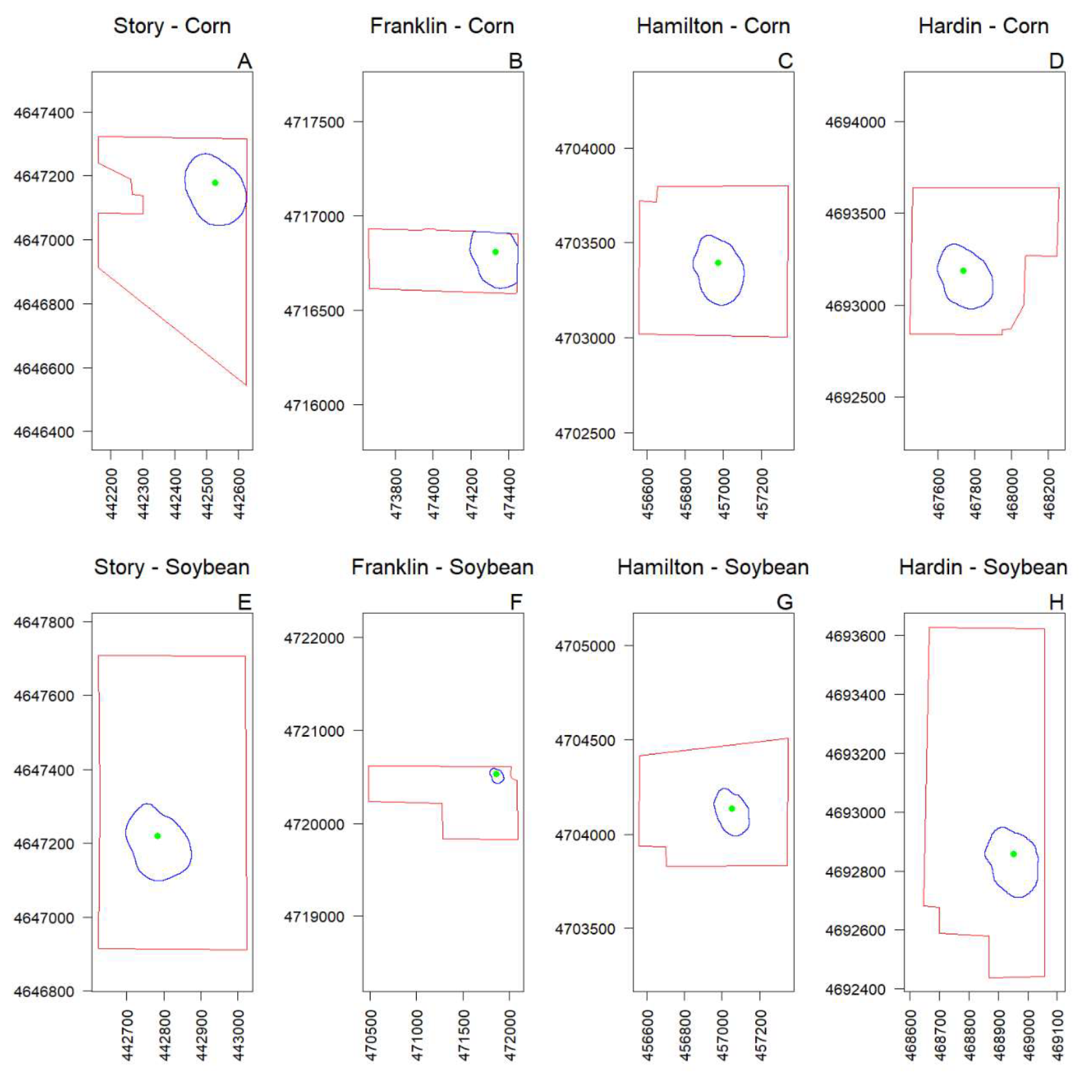
Appendix A. Flux Footprints

Figure A1. The average 90% flux footprint area (blue borders) of each EC station (green circles) within corn (AD) and soybean (EH) fields (red borders) in Story, Franklin, Hamilton, and Hardin County, Iowa.
Remotesensing 11 01688 g0a1

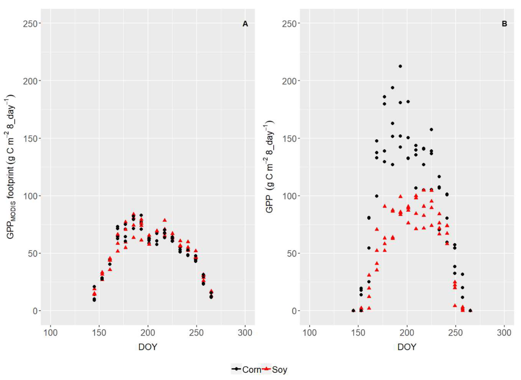
Appendix B. MODIS GPP Product vs. Field-Measured GPP

Figure A2. The gross primary production (GPP) averaged for corn (black circles, n=4) and soybean (red triangles, n=4) in four counties in North Central Iowa during the 2016 growing season (DOY 145–269); (A) The 8-day GPPMODIS product (g C m−2 8-day−1) within the 90% footprint area of the EC station. (B) The 8-day-sum of EC-derived GPP (g C m−2 8-day−1).
Remotesensing 11 01688 g0a2
Figure A3. Daily GPPMODIS product (g C m−2 d−1) on DOY 193 in 2016 for four Iowa counties. Triangles and circles show the location of the eddy covariance (EC) stations in soybean and corn fields, respectively.
Remotesensing 11 01688 g0a3

References

  1. National Agricultural Statistics Service (NASS). Available online: https://www.nass.usda.gov/Publications/Ag_Statistics/index.php (accessed on 4 April 2019).
  2. FAOSTAT. Food and Agriculture Organization of the United Nations, Statistics Division. Forestry Production and Trade. Available online: http://www.fao.org/faostat/en/#data/FO (accessed on 4 April 2019).
  3. Guanter, L.; Zhang, Y.; Jung, M.; Joiner, J.; Voigt, M.; Berry, J.A.; Frankenberg, C.; Huete, A.R.; Zarco-Tejada, P.J.; Lee, J.E.; et al. Global and time-resolved monitoring of crop photosynthesis with chlorophyll fluorescence. Proc. Natl. Acad. Sci. USA 2014, 111, E1327–E1333. [Google Scholar] [CrossRef] [PubMed] [Green Version]
  4. Dold, C.; Hatfield, J.L.; Prueger, J.H.; Sauer, T.J.; Moorman, T.B.; Wacha, K.M. Impact of Management Practices on Carbon and Water Fluxes in Corn–Soybean Rotations. AGE 2019, 2, 1–8. [Google Scholar] [CrossRef]
  5. USDA-NASS. 2017 Census of Agriculture. Available online: https://www.nass.usda.gov/Publications/AgCensus/2017/Full_Report/Volume_1,_Chapter_1_State_Level/Iowa/ (accessed on 9 July 2019).
  6. Running, S.W.; Zhao, M. Daily GPP and Annual NPP (MOD17A2/A3) Products NASA Earth Observing System MODIS Land Algorithm. Version 3.0; 2015; p. 28. Available online: https://landweb.modaps.eosdis.nasa.gov/QA_WWW/forPage/user_guide/MOD17UsersGuide2015v3.pdf (accessed on 19 March 2019).
  7. Reeves, M.C.; Zhao, M.; Running, S.W. Usefulness and limits of MODIS GPP for estimating wheat yield. Int. J. Remote Sens. 2005, 26, 1403–1421. [Google Scholar] [CrossRef]
  8. Ryu, Y.; Baldocchi, D.D.; Kobayashi, H.; Van Ingen, C.; Li, J.; Black, T.A.; Beringer, J.; Van Gorsel, E.; Knohl, A.; Law, B.E.; et al. Integration of MODIS land and atmosphere products with a coupled-process model to estimate gross primary productivity and evapotranspiration from 1 km to global scales. Glob. Biogeochem. Cycles 2011, 25, 25. [Google Scholar] [CrossRef]
  9. Jiang, C.; Ryu, Y. Multi-scale evaluation of global gross primary productivity and evapotranspiration products derived from Breathing Earth System Simulator (BESS). Remote Sens. Environ. 2016, 186, 528–547. [Google Scholar] [CrossRef]
  10. Coops, N.; Black, T.; Jassal, R.; Trofymow, J.; Morgenstern, K. Comparison of MODIS, eddy covariance determined and physiologically modelled gross primary production (GPP) in a Douglas-fir forest stand. Remote Sens. Environ. 2007, 107, 385–401. [Google Scholar] [CrossRef]
  11. Wu, C.; Munger, J.W.; Niu, Z.; Kuang, D. Comparison of multiple models for estimating gross primary production using MODIS and eddy covariance data in Harvard Forest. Remote Sens. Environ. 2010, 114, 2925–2939. [Google Scholar] [CrossRef]
  12. Xin, Q.; Broich, M.; Suyker, A.E.; Yu, L.; Gong, P. Multi-scale evaluation of light use efficiency in MODIS gross primary productivity for croplands in the Midwestern United States. Agric. For. Meteorol. 2015, 201, 111–119. [Google Scholar] [CrossRef] [Green Version]
  13. Xin, Q.; Gong, P.; Yu, C.; Yu, L.; Broich, M.; Suyker, A.E.; Myneni, R.B. A Production Efficiency Model-Based Method for Satellite Estimates of Corn and Soybean Yields in the Midwestern US. Remote Sens. 2013, 5, 5926–5943. [Google Scholar] [CrossRef] [Green Version]
  14. Zhang, Q.; Cheng, Y.-B.; Lyapustin, A.I.; Wang, Y.; Gao, F.; Suyker, A.; Verma, S.; Middleton, E.M. Estimation of crop gross primary production (GPP): fAPARchl versus MOD15A2 FPAR. Remote Sens. Environ. 2014, 153, 1–6. [Google Scholar] [CrossRef] [Green Version]
  15. Zhang, Q.; Cheng, Y.B.; Lyapustin, A.I.; Wang, Y.; Zhang, X.; Suyker, A.; Verma, S.; Shuai, Y.; Middleton, E.M. Estimation of crop gross primary production (GPP): II. Do scaled MODIS vegetation indices improve performance? Agric. For. Meteorol. 2015, 200, 1–8. [Google Scholar] [CrossRef] [Green Version]
  16. Sjöström, M.; Zhao, M.; Archibald, S.; Arneth, A.; Cappelaere, B.; Falk, U.; De Grandcourt, A.; Hanan, N.; Kergoat, L.; Kutsch, W.; et al. Evaluation of MODIS gross primary productivity for Africa using eddy covariance data. Remote Sens. Environ. 2013, 131, 275–286. [Google Scholar] [CrossRef]
  17. Turner, D.P.; Ritts, W.D.; Cohen, W.B.; Gower, S.T.; Running, S.W.; Zhao, M.; Costa, M.H.; Kirschbaum, A.A.; Ham, J.M.; Saleska, S.R.; et al. Evaluation of MODIS NPP and GPP products across multiple biomes. Remote Sens. Environ. 2006, 102, 282–292. [Google Scholar] [CrossRef]
  18. Tomer, M.D.E.; James, D.; Sandoval-Green, C.M.J. Agricultural Conservation Planning Framework: 3. Land Use and Field Boundary Database Development and Structure. J. Environ. Qual. 2017, 46, 676–686. [Google Scholar] [CrossRef] [PubMed] [Green Version]
  19. Cosh, M.H.; White, W.A.; Colliander, A.; Jackson, T.J.; Prueger, J.H.; Hornbuckle, B.K.; Hunt, E.R.; McNairn, H.; Powers, J.; Walker, V.A.; et al. Estimating vegetation water content during the Soil Moisture Active Passive Validation Experiment 2016. J. Appl. Remote Sens. 2019, 13, 014516. [Google Scholar] [CrossRef]
  20. Colliander, A.; Cosh, M.H.; Misra, S.; Jackson, T.J.; Crow, W.T.; Powers, J.; McNairn, H.; Bullock, P.; Berg, A.; Magagi, R.; et al. Comparison of high-resolution airborne soil moisture retrievals to SMAP soil moisture during the SMAP validation experiment 2016 (SMAPVEX16). Remote Sens. Environ. 2019, 227, 137–150. [Google Scholar] [CrossRef]
  21. USDA-NRCS. Soil Survey Geographic (SSURGO) Database for Hardin, Franklin, Hamilton & Story County, Iowa; Soil Survey Staff, Natural Resources Conservation Service, United States Department of Agriculture: Washington, DC, USA, 2018.
  22. IEM. Iowa Environmental Mesonet—Climate Data. Available online: https://mesonet.agron.iastate.edu/ (accessed on 10 October 2018).
  23. Burba, G. Eddy Covariance Method for Scientific, Industrial, Agricultural and Regulatory Applications: A Field Book on Measuring Ecosystem Gas. Exchange and Areal Emission Rates; LI-COR Biosciences: Lincoln, NE, USA, 2013; p. 331. [Google Scholar]
  24. Kljun, N.; Calanca, P.; Rotach, M.W.; Schmid, H.P. A simple two-dimensional parameterisation for Flux Footprint Prediction (FFP). Geosci. Model. Dev. 2015, 8, 3695–3713. [Google Scholar] [CrossRef] [Green Version]
  25. Tanner, C.B.; Thurtell, G.W. Anemoclinometer Measurements of Reynolds Stress and Heat Transport in the Atmospheric Surface Layer; Department of Soil Science Wisconsin University: Madison, WI, USA, 1969; pp. 1–10. [Google Scholar]
  26. Webb, E.; Pearman, G.; Leuning, R. Correction of flux measurements for density effects due to heat and water vapour transfer. Q. J. R. Meteorol. Soc. 1980, 106, 85–100. [Google Scholar] [CrossRef]
  27. Dold, C.; Büyükcangaz, H.; Rondinelli, W.; Prueger, J.; Sauer, T.; Hatfield, J. Long-term carbon uptake of agro-ecosystems in the Midwest. Agric. For. Meteorol. 2017, 232, 128–140. [Google Scholar] [CrossRef] [Green Version]
  28. Hernandez-Ramirez, G.; Hatfield, J.L.; Parkin, T.B.; Sauer, T.J.; Prueger, J.H. Carbon dioxide fluxes in corn–soybean rotation in the midwestern U.S.: Inter- and intra-annual variations, and biophysical controls. Agric. For. Meteorol. 2011, 151, 1831–1842. [Google Scholar] [CrossRef]
  29. Baker, J.; Griffis, T. Examining strategies to improve the carbon balance of corn/soybean agriculture using eddy covariance and mass balance techniques. Agric. For. Meteorol. 2005, 128, 163–177. [Google Scholar] [CrossRef]
  30. Hernandez-Ramirez, G.; Hatfield, J.L.; Prueger, J.H.; Sauer, T.J. Energy balance and turbulent flux partitioning in a corn–soybean rotation in the Midwestern US. Theor. Appl. Climatol. 2010, 100, 79–92. [Google Scholar] [CrossRef]
  31. Reichstein, M.; Falge, E.; Baldocchi, D.; Papale, D.; Aubinet, M.; Berbigier, P.; Bernhofer, C.; Buchmann, N.; Gilmanov, T.; Granier, A.; et al. On the separation of net ecosystem exchange into assimilation and ecosystem respiration: Review and improved algorithm. Glob. Chang. Boil. 2005, 11, 1424–1439. [Google Scholar] [CrossRef]
  32. Gilmanov, T.; Soussana, J.-F.; Aires, L.M.I.; Allard, V.; Ammann, C.; Balzarolo, M.; Barcza, Z.; Bernhofer, C.; Campbell, C.; Cernusca, A.; et al. Partitioning European grassland net ecosystem CO2 exchange into gross primary productivity and ecosystem respiration using light response function analysis. Agric. Ecosyst. Environ. 2007, 121, 93–120. [Google Scholar] [CrossRef]
  33. Campbell, G.S.; Norman, J.M. An Introduction to Environmental Biophysics; Springer Science and Business Media LLC: New York, NY, USA, 1998; p. 286. [Google Scholar]
  34. Hatfield, J.L. Radiation Use Efficiency: Evaluation of Cropping and Management Systems. Agron. J. 2014, 106, 1820. [Google Scholar] [CrossRef]
  35. Hatfield, J.L.; Prueger, J.H. Value of Using Different Vegetative Indices to Quantify Agricultural Crop Characteristics at Different Growth Stages under Varying Management Practices. Remote Sens. 2010, 2, 562–578. [Google Scholar] [CrossRef] [Green Version]
  36. Abendroth, L.J.; Elmore, R.W.; Boyer, M.J.; Marlay, S.K. Corn Growth and Development; PMR: Ames, IA, USA, Iowa State University Extension; 2011. [Google Scholar]
  37. Pedersen, P. Soybean Growth and Development; Iowa State University: Ames, IA, USA, 2004. [Google Scholar]
  38. USGS. US Geological Survey, MODIS Products Courtesy of the U.S. Geological Survey. Available online: https://lpdaacsvc.cr.usgs.gov/appeears/ (accessed on 21 March 2019).
  39. Myneni, R.; Knyazikhin, Y.; Park, T. MOD15A2H MODIS/Terra Leaf Area Index/FPAR 8-Day L4 Global 500 m SIN Grid V006 [Dataset]. Available online: http://doi.org/10.5067/MODIS/MOD15A2H.006 (accessed on 10 October 2018).
  40. Lowe, P.R. An Approximating Polynomial for the Computation of Saturation Vapor Pressure. J. Appl. Meteorol. 1977, 16, 100–103. [Google Scholar] [CrossRef] [Green Version]
  41. R Core Team. The R Foundation for Statistical Computing; The R Foundation: Vienna, Austria, 2014. [Google Scholar]
  42. Friedl, M.; Sulla-Menashe, D. MCD12Q1 MODIS/Terra+ Aqua Land Cover Type Yearly L3 Global 500m SIN Grid V006 [Dataset]. Available online: http://doi.org/10.5067/MODIS/MCD12C1.006 (accessed on 10 October 2018).
  43. Pedersen, P.; Lauer, J.G. Response of Soybean Yield Components to Management System and Planting Date. Agron. J. 2004, 96, 1372. [Google Scholar] [CrossRef]
  44. Karlen, D.L.; Kovar, J.L.; Birrell, S.J. Corn Stover Nutrient Removal Estimates for Central Iowa, USA. Sustainability 2015, 7, 8621–8634. [Google Scholar] [CrossRef] [Green Version]
  45. Prince, S.D.; Haskett, J.; Steininger, M.; Strand, H.; Wright, R. Net primary production of US Midwest croplands from agricultural harvest yield data. Ecol. Appl. 2001, 11, 1194–1205. [Google Scholar] [CrossRef]
  46. Bernacchi, C.J.; Hollinger, S.E.; Meyers, T. The conversion of the corn/soybean ecosystem to no-till agriculture may result in a carbon sink. Glob. Chang. Boil. 2005, 11, 1867–1872. [Google Scholar] [CrossRef]
  47. Hatfield, J.L.; Prueger, J.H.; Kustas, W.P. Spatial and Temporal Variation of Energy and Carbon Fluxes in Central Iowa. Agron. J. 2007, 99, 285. [Google Scholar] [CrossRef]
  48. Sainju, U.M.; Jabro, J.D.; Stevens, W.B. Soil Carbon Dioxide Emission and Carbon Content as Affected by Irrigation, Tillage, Cropping System, and Nitrogen Fertilization. J. Environ. Qual. 2008, 37, 98. [Google Scholar] [CrossRef] [PubMed]
  49. Kanamitsu, M.; Ebisuzaki, W.; Woollen, J.; Yang, S.-K.; Hnilo, J.J.; Fiorino, M.; Potter, G.L. NCEP–DOE AMIP-II Reanalysis (R-2). Bull. Am. Meteorol. Soc. 2002, 83, 1631–1644. [Google Scholar] [CrossRef]
Figure 1. Land use map of four counties in Iowa (red marked counties in small map) in 2016 [18]: Story County (lower), Hamilton County (center left), Hardin County (center right), and Franklin County (upper). Corn fields are marked dark green, and soybean fields are light green (each land use area > 55%). The red triangles and yellow circles show the location of the eddy-covariance (EC) stations in soybean and corn fields, respectively.
Remotesensing 11 01688 g001
Figure 2. Meteorological data and carbon fluxes for the 2016 growing season in four Iowan counties: (A) Daily incoming photosynthetic active radiation (IPAR, MJ m−2 d−1), (B) daily ambient air temperature (Ta, °C), and (C) daytime vapor pressure deficit (VPD, kPa) averaged (± SE) over eight eddy-flux stations. In addition, (D) daily gross primary production (GPP, g C m−2 d−1), (E) daily net ecosystem production (NEP, g C m−2 d−1), and (F) ecosystem respiration (RE, g C m−2 d−1) averaged over crop (n = 4); red triangles for soybean and black circles for corn.
Remotesensing 11 01688 g002
Figure 3. Measurements on the corn (black circles) and soybean (red triangles) field in Story County during the 2016 growing season ; (A) measured and interpolated corn and soybean NDVI near the eddy-flux stations; (B) linear regression analysis (p < 0.05) with measured NDVI as independent and MODIS fPAR in the 90% footprint area as dependent variable; (C) linear regression analysis (p < 0.05) with the product of the Tmins, VPDs, NDVI, and IPAR (MJ m−2 d−1) as independent and GPP (g C m−2 d−1) as dependent variable with the slope being RUEmax. R2: coefficient of determination, Tmins: temperature scalar, VPDs: vapor pressure deficit scalar, IPAR: incoming photosynthetic active radiation, GPP: gross primary production, RUEmax: maximum radiation use efficiency.
Remotesensing 11 01688 g003
Figure 4. MODIS fPAR product (MCD15A2H) for DOY 193 in 2016 in four Iowan counties for corn and soybean fields. The red triangles and yellow circles show the location of the eddy covariance (EC) stations on soybean and corn fields, respectively; fPAR: fraction of absorbed photosynthetic active radiation.
Remotesensing 11 01688 g004
Figure 5. GPPcalc as calculated with MODIS fPAR product for corn (black circles) and soybean (red triangles) for 2016: (A) median county fPAR, averaged (± SE) over county (n = 4), (B) daily median county GPPcalc (g C M−2 d−1) averaged over county, and (C) linear regression analysis (p < 0.05) with daily EC-derived GPP as independent and 90% footprint GPPcalc (g C m−2 d−1) as dependent variable, R2: coefficient of determination, GPP: gross primary production, fPAR: fraction of absorbed photosynthetic active radiation.
Remotesensing 11 01688 g005
Figure 6. Daily GPPcalc (g C m−2 d−1) on DOY 193 in 2016 for four Iowa counties. Triangles and circles show the location of the eddy covariance (EC) stations in soybean and corn fields, respectively.
Remotesensing 11 01688 g006
Table 1. Site specifics (location, soils, crop management) and EC station instrumentation (sonic, IRGA, and radiation specifics, measurement height, measurement frequency, and sonic direction).
CountyStoryFranklinHamiltonHardin
Ameriflux codeUS-Br1US-Br3------------------
CropCornSoybeanCornSoybeanCornSoybeanCornSoybean
Latitude,
Longitude (dec. °)
41.975,−93.69441.975,−93.69142.603,−93.31342.637,−93.34342.482,−93.52442.488,−93.52342.390,−93.39242.387,−93.377
Field size (ha)31.525.8119.294.147.560.828.844.0
Soil type and texture 1Canisteo, Harps, Okoboji,
loam–clay loam
Harps, Okoboji, Zenor, Storden, Salida, Coland, Lawler
sandy loam–clay loam
Harps, Okoboji
loam–clay loam
Storden, Okoboji, Harps, Coland
loam–clay loam
Soil managementSpring tillage; fall tillageSpring tillageSpring tillage; fall tillageSpring tillageSpring tillageNANo dataNo data
N-rate
(kg N ha−1 year−1)
Anhydrous-N: 168NANo dataNo dataNH3/UAN: 157NANo dataNo data
Density (plants ha−1)80,000379,00083,200309,00078,600323,00092,900No data
Planting–Harvest DOY111–271128–292140–271144–270128–273115–282138–298144–275
IRGA modelLI-7500 2EC150 3IRGASON 3LI-7500 2
3-D Sonic anemometer modelCSAT-3 3EC150 3IRGASON 3CSAT-3 3
zm (cm)240–500225200–500200200–500200–240200–500218–240
Frequency (Hz)20
Azimuth
from North
270°
Radiation
sensor model
CNR-1 4CNR-4 4NR-01 5CNR-1 4
Sonic = 3-D sonic anemometer, IRGA = infrared gas analyzer, zm = measurement height. 1 retrieved from soil descriptions [14]. 2 LICOR Biosciences Inc., Lincoln, NE, USA. 3 Campbell Scientific, Inc., Logan, UT, USA. 4 Kipp & Zonen, Delft, The Netherlands. 5 Hukseflux, Delft, The Netherlands
Table 2. Seasonal (DOY 145–269) NEP, RE, and GPP as well as Yield [1] and calculated YieldGPP, averaged (± SE) over four Iowa counties for corn and soybean (n = 4) in 2016.
CropVariableNEP
(g C m−2)
RE
(g C m−2)
GPP
(g C m−2)
YieldGPP
(Mg ha−1)
Yield (NASS)
(Mg ha−1)
CornMean ± SE678 ± 63−805 ± 401483 ± 10012.82 ± 0.6513.09 ± 0.09
95% CI[547,769][−897,−779][1334,1655]------
SoybeanMean ± SE263 ± 40−548 ± 14811 ± 536.73 ± 0.274.03 ± 0.04
95% CI[170,318][−602,−531][728,913]------
NEP = net ecosystem production, GPP = gross primary production, RE = ecosystem respiration, YieldGPP = yield as calculated with Equation (6).

